


1. Introduction
Hydrophobicity – defined to be water-repelling, anti-mixing or non-wetting behaviour – is a feature that has found applications in many areas of modern science. An extreme example is that of fluid suspended over multiple gas cavities, which are created by microscopic surface roughness (namely, pillars or ridges). Such structures are characterised as superhydrophobic if a fluid droplet at rest possesses a liquid–solid contact angle greater than  $150^\circ$ and take much of their inspiration from nature (Wang & Jiang Reference Wang and Jiang2007). As an example, the lotus leaf employs it as a tool for self-cleaning, to improve and regulate photosynthesis. In the context of a channel flow, depending on the size and shape of these structures, the liquid may exist in a suspended Cassie–Baxter state (Cassie & Baxter Reference Cassie and Baxter1944). Here, the fluid is in contact only with solid maxima, hence exhibiting an effective slip over the gas phase; the bulk flow is therefore lubricated and a reduction in the viscous drag follows (Rothstein Reference Rothstein2010). Loss of the Cassie–Baxter state produces the Wenzel state (Marmur Reference Marmur2003), with the liquid partially or completely filling the grooves. Since these types of surfaces have significantly fewer applications they are not considered from this point onwards.
Experiments by Ou, Perot & Rothstein (Reference Ou, Perot and Rothstein2004), Ou & Rothstein (Reference Ou and Rothstein2005), Davies et al. (Reference Davies, Maynes, Webb and Woolford2006) and Choi & Kim (Reference Choi and Kim2006) provided evidence of drag reduction in laminar flows over superhydrophobic surfaces (SHSs) due to a marked reduction in required applied pressure gradients or torque relative to what is required for smooth solid surfaces. More recent experiments include those by Peaudecerf et al. (Reference Peaudecerf, Landel, Goldstein and Luzzatto-Fegiz2017) and Song et al. (Reference Song, Song, Hu, Du, Du, Choi and Rothstein2018), who pay particular attention to surfactant-induced Marangoni effects. Song et al. (Reference Song, Song, Hu, Du, Du, Choi and Rothstein2018) built and studied circular Couette microchannels with annular grooves in order to produce a physical model to compare with the theory and to control the effects of baffles. A fundamental study into turbulent superhydrophobic (SH) flows was undertaken by Min & Kim (Reference Min and Kim2004), who used direct numerical simulations (DNS) with Navier-slip boundary conditions at the walls. Their results indicate that drag reduction is achieved for longitudinal ridges, due to a weakening of the turbulence intensity and damping of vortical structures. Martell, Perot & Rothstein (Reference Martell, Perot and Rothstein2009) used DNS to examine SHSs in a turbulent channel flow and enforced the correct stick-slip boundary conditions. Daniello, Waterhouse & Rothstein (Reference Daniello, Waterhouse and Rothstein2009) used particle image velocimetry and pressure drop measurements to estimate drag reductions of the order of 50 %.
The majority of theoretical work in this field considers laminar unperturbed flows whose stability we seek to analyse. Historically two types of flows have been considered. Those with transverse grooves perpendicular to the flow direction, and flows with longitudinal grooves parallel to the flow direction. We are concerned with applications described by the latter class as they generally induce greater reductions in drag – for studies involving transversely oriented ridges the reader is referred to Davis & Lauga (Reference Davis and Lauga2009), Crowdy (Reference Crowdy2017b), Landel et al. (Reference Landel, Peaudecerf, Temprano-Coleto, Gibou, Goldstein and Luzzatto-Fegiz2020) and references therein. A schematic of the longitudinal flow of interest here can be found in figure 1. Theoretical studies involving longitudinal grooves are mostly concerned with three canonical cases: (i) constant unbounded shear flows over SHSs, (ii) Couette flows where the bottom plate is structured and the top one is moving at a constant speed and (iii) channel flows driven by a constant pressure gradient with one or both of the plates structured.

Figure 1. Schematics of the problem: (a) depicts the general picture (a SHS for the bottom plate and a solid top wall), and (b) the non-dimensional domain,  $\mathcal {D}$, by means of the physical assumptions made and symmetry conditions. In (b),
  $h$ is the non-dimensional channel height,
  $\delta$ is the slip fraction and the dashed line denotes one period. Lastly, the dark grey areas indicate the solid boundary, the light blue the modelled fluid and the white the external gas region.
The seminal work by Philip (Reference Philip1972) analysed a unbounded shear flow with flat menisci both for transverse grooves (in the absence of inertia), and longitudinal grooves in which case the resulting flow aligned with the shear is an exact solution of the Navier–Stokes equations that depends on the cross-plane coordinates. This work was followed by Lauga & Stone (Reference Lauga and Stone2003) and Teo & Khoo (Reference Teo and Khoo2009), who used separation of variables and dual series techniques, in both cases ignoring meniscus curvature that does not conform with the ridge geometry. Meniscus curvature was first included by Sbragaglia & Prosperetti (Reference Sbragaglia and Prosperetti2007) for longitudinal grooves in a Couette channel flow, by developing a weakly curved meniscus asymptotic analysis about a flat configuration, and producing corrections to Philip's results for the slip lengths. Such domain perturbation methods were also applied to diabatic pressure-driven SHSs – see Kirk, Hodes & Papageorgiou (Reference Kirk, Hodes and Papageorgiou2017) – and later extended numerically to arbitrary curvatures by Game et al. (Reference Game, Hodes, Kirk and Papageorgiou2018). The powerful complex analysis tools utilised by Philip were developed further, and for different geometries notably allowing for curved menisci, see Crowdy (Reference Crowdy2015, Reference Crowdy2016, Reference Crowdy2017b), Marshall (Reference Marshall2017) and Luca, Marshall & Karamanis (Reference Luca, Marshall and Karamanis2018). Further extensions allowing for diabatic effects have also been carried out – Yariv & Crowdy (Reference Yariv and Crowdy2020) and Yariv & Kirk (Reference Yariv and Kirk2021).
All of the studies described above ignore the effect of the gas present in the grooves, resulting in a zero shear boundary condition on the meniscus. Inclusion of gas effects have been considered numerically (and compared with available experiments) by Davies et al. (Reference Davies, Maynes, Webb and Woolford2006), Maynes, Webb & Davies (Reference Maynes, Webb and Davies2008), Woolford, Maynes & Webb (Reference Woolford, Maynes and Webb2009) and also by Ng & Wang (Reference Ng and Wang2009) using eigenfunction expansions for their computations; all these studies assume flat menisci with no streamwise variation. Additional analytical explorations for flat menisci have been considered by Schönecker & Hardt (Reference Schönecker and Hardt2013) and Schönecker, Baier & Hardt (Reference Schönecker, Baier and Hardt2014), where effective constant shear boundary conditions were used to approximate the effect of the gas region. Keeping with flat menisci and seeking effective models to lump the gas-region presence into an effective boundary condition, has enabled Asmolov & Vinogradova (Reference Asmolov and Vinogradova2012) and Nizkaya, Asmolov & Vinogradova (Reference Nizkaya, Asmolov and Vinogradova2014) to propose approximate solutions such as what they call the ‘gas cushion model’. Crowdy (Reference Crowdy2017a) considered the full equations of motion for pressure-driven flow with open groove ends, and carried out an asymptotic analysis combining small meniscus deflection coupled with a small viscosity ratio. More recent computational studies have been carried out by Game et al. (Reference Game, Hodes, Keaveny and Papageorgiou2017), who accounts fully for the effects of the gas region and arbitrary meniscus curvature using domain decomposition spectral methods. Following Davies et al. (Reference Davies, Maynes, Webb and Woolford2006), they took the gas pocket region to be closed at the channel entrance and exit, producing a mass-conserving recirculating zone whose pressure is determined as part of the solution inducing drag on the main channel flow.
Almost all theoretical studies to date do not account for three-dimensionality. This is both due to the complexity of the problem and the limited possibilities for DNS parameter studies. However, the underlying physics suggests that the menisci vary weakly in the streamwise direction with small deflections, as detailed next. Considering pressure-driven flows, the larger pressure at the inlet induces the largest meniscus deflection there, and this relaxes to a flat state as the channel is traversed, assuming that the outflow is open to ambient conditions. However, the length of the channel is typically long compared with the ridge pitch (equivalently the spacing between ridges). In the experiments of Ou et al. (Reference Ou, Perot and Rothstein2004) and Ou & Rothstein (Reference Ou and Rothstein2005), the length is  $L=50$ mm while the distance between ridges ranges from 20 to
  $120\ \mathrm {\mu }\textrm {m}$. Half-way down the channel, the experiments find deflections of the order of
  $3\ \mathrm {\mu }\textrm {m}$ or less for a ridge pitch of approximately
  $60\ {\rm \mu}$m, hence the ratio of deflection to ridge pitch is
  $\epsilon _{sp} \approx 0.05$, that is sufficiently small to expect theories such as in Sbragaglia & Prosperetti (Reference Sbragaglia and Prosperetti2007) to be valid. Additional support for a small deflection parameter is given here following Kirk et al. (Reference Kirk, Hodes and Papageorgiou2017). Taking water on a low-surface-energy fluoropolymer that has a maximum protrusion angle of
  $20^\circ$ into the cavity, and additionally taking a low dimensionless solid fraction of
  $0.01$ (where the solid fraction is defined by the ratio of the ridge width to the pitch), gives a maximum deflection parameter of
  $\epsilon _{sp} \approx 0.17$, again within the limits of asymptotic approximations. Returning to the experiments of Ou et al. (Reference Ou, Perot and Rothstein2004) and Ou & Rothstein (Reference Ou and Rothstein2005), the ratio of ridge pitch to length is of the order of
  $\epsilon :\approx 10^{-3}$. Even for meniscus curvatures that are not small it is reasonable to assume that the undisturbed state will vary weakly in the streamwise direction, and the fact
  $\epsilon \ll 1$ opens the way for a rational asymptotic analysis that can fully account for three-dimensionality in certain applications. Such analyses were undertaken by Game, Hodes & Papageorgiou (Reference Game, Hodes and Papageorgiou2019) without assuming small deflections. A solution is built by computing numerically the cross-flow quasi-uniform solution at each streamwise location if the pressure at that location is known, and coupling this to the determination of the pressure from streamwise flux conservation.
The objective of the present work is to investigate the stability of flows in SHSs for different parameters, with the aim of explaining some experimental observations that find differences between measurements and steady laminar flow theories. The full three-dimensional problem will not be considered due to its complexity and its tri-global stability nature. Noting the slowly varying nature of the underlying flows, we proceed with a detailed study of bi-global stability problems, and indeed the simpler class of flat meniscus ones. There are two reasons that justify this: (i) meniscus curvature is small in many situations (see above), and (ii) the quasi-uniform approach is completely consistent with the results reported here. The latter statement is quantified fully in this paper, but briefly, with our non-dimensionalisation using the ridge pitch for lengths, we compute the most unstable wavenumbers to be of order unity, implying that their physical length is of the order of the pitch, and hence short compared with the channel length over which the three-dimensionality develops. Our numerical methods apply equally to arbitrarily curved menisci – indeed computations to be reported elsewhere also predict  $O(1)$ wavenumbers. The underlying instabilities are inherently present due to the two-dimensional flow structure in the cross-plane and not due to finer details of meniscus curvature or a modified shear stress that accounts for gas effects (this would undoubtedly affect the growth rates and would be of considerable interest in the future).
Bi-global stability problems have been considered previously for rectangular duct flows (Tatsumi & Yoshimura Reference Tatsumi and Yoshimura1990), flows over riblets (Ehrenstein Reference Ehrenstein1996) and shear flows with distributed wall roughness (Floryan Reference Floryan1997), to mention some of the earliest ones. Theofilis, Duck & Owen (Reference Theofilis, Duck and Owen2004) revisited the duct flow results of Tatsumi & Yoshimura (Reference Tatsumi and Yoshimura1990) and examined three other two-dimensional basic profiles. Moradi & Floryan (Reference Moradi and Floryan2014) investigated a channel flow with wavy walls, where they discover a critical groove wavenumber that can stabilise or destabilise the planar flow. In an extension of this to grooved channels, Mohammadi, Moradi & Floryan (Reference Mohammadi, Moradi and Floryan2015) report an inviscidly unstable mode which is excited in this configuration (indeed, they predict that this mode is excited for any spanwise structuring). They connect the viscous and inviscid modes to the Orr–Sommerfeld and Squire modes of plane Poiseuille flow. These modes are analogous to the ones we find in this study where the solid walls are replaced by stick-slip surfaces pertinent to SHSs. Their existence in two quite different flows provides strong evidence that it is the cross-plane variation of the basic flow that underpins the instabilities rather than finer details such as meniscus curvature. For completeness, we point out inviscid bi-global stability studies by Hall & Horseman (Reference Hall and Horseman1991) who considered the stability of longitudinal vortices in boundary layers, and Duck (Reference Duck2011) who examined the breakdown of trailing line vortices. Tri-global stability problems lie outside the scope of this study, as do weakly varying or other parabolic stability type techniques. More details and an in-depth review of other global stability problems can be found in Theofilis (Reference Theofilis2003). Examples of tri-global stability studies include Bagheri et al. (Reference Bagheri, Schlatter, Schmid and Henningson2009), who investigated the global stability of a jet in a cross-flow, and Loiseau et al. (Reference Loiseau, Robinet, Cherubini and Leriche2014) and Bucci et al. (Reference Bucci, Puckert, Andriano, Loiseau, Cherubini, Robinet and Rist2018), who examined the global stability of a cylindrical roughness element in a boundary layer.
Initial attempts to study the stability of SHS flows centred on replacing the mixed boundary condition with a Navier-slip condition. Plane Poiseuille flow (PPF) was studied by Lauga & Cossu (Reference Lauga and Cossu2005), who find an increase in critical Reynolds number due to the modified condition, but a very weak influence in the non-modal stability characteristics. More recently, Pralits, Alinovi & Bottaro (Reference Pralits, Alinovi and Bottaro2017) model an oblique flow over SHSs by introducing a slip tensor and carrying out a stability analysis of the resulting basic flow. Once again the details of the spanwise base flow variations are absent. The instability modes reported by us would not be picked up by a stability analysis that uses a slip boundary condition. The use of such conditions renders the basic profile one-dimensional without the spanwise structure that induces the instability modes reported here. Indeed, the lid-driven problem would be neutrally stable and the unstable mode of PPF would merely be perturbed by the imposed slip length rather than supporting lower Reynolds number inflectional instabilities. More accurate boundary conditions were implemented by Yu, Teo & Khoo (Reference Yu, Teo and Khoo2016) in a pressure-driven channel, with either one or two SHSs, resulting in the appropriate bi-global stability problem. For large channel heights, their results agree with those arising from the PPF analysis. For small channel heights stabilisation is predicted, and as we show here this is due to their implementation of an inviscid boundary condition This assumption does not allow for the detection of the viscously unstable modes found in § 6.4. More recently, DNS of the laminar–turbulent transitional state has been undertaken by Picella, Robinet & Cherubini (Reference Picella, Robinet and Cherubini2019) initially using effective Navier-slip boundary conditions. They study the evolution of both modal and non-modal disturbances, and show that SHS may be used to delay transition in the former and have no effect on the latter. Extending these works, Picella, Robinet & Cherubini (Reference Picella, Robinet and Cherubini2020) then impose correct mixed boundary conditions to study the effects of the interface dynamics on transition. They find that transition again occurs further downstream, however, the stabilisation effects are reduced relative to the slip conditions.
This work provides an accurate numerical procedure for solving generalised eigenvalue problems (GEVPs) that arise in SHS flows with mixed boundary conditions. Results are presented for lid- and pressure-driven flows, expanding on the current understanding of the instability of such flows.
The rest of the paper is arranged as follows. In § 2, the channel geometry is introduced and the linear stability problem formulated. In § 3, the background flow field is solved for both configurations. In § 4, the stability analysis is performed (this includes singularity removal), resulting in a GEVP which is solved in both its viscous and inviscid formulations. Section 5 provides the discretisation using Chebyshev collocation and domain deposition. Section 6 presents and analyses the viscous stability results for both pressure- and lid-driven flows. This includes a link to the plane flow, inviscid instability problem and a comparison with experimental results. Finally, in § 7, we draw some conclusions and outline some extensions and implications of this work.
2. Governing equations and problem formulation
We consider the linear stability of laminar flow over a SHS which has regularly spaced grooves aligned in the streamwise direction – see figure 1(a). Two configurations will be considered. First, a Couette flow which is driven by an unstructured upper lid moving with velocity  $U_c^*$ over a SHS. This we term as superhydrophobic Couette (SHSC) flow. The second is driven by a constant pressure gradient
  $-G_p^*$ over a SHS. Such flows can be found in pipes or channels and will be referred to as superhydrophobic Poiseuille (SHSP) flow. As a starting point for such complex flows, the liquid is taken to be in the Cassie–Baxter state. Furthermore, we take the liquid–gas interface to be flat (work is underway to generalise our results to curved menisci). For a study of the basic flows emerging in the presence of curved menisci see Game et al. (Reference Game, Hodes, Keaveny and Papageorgiou2017, Reference Game, Hodes and Papageorgiou2019). One may exploit the spanwise periodicity of the problem across the ridges (we assume that there is a large number of them), and restrict the domain by symmetry to one-half period. We then define a Cartesian coordinate frame located at the top and centre of the gas cavity, such that
  $\boldsymbol {r}^*\equiv (x^*,y^*,z^*)$;
  $x^*$ is taken to be in the streamwise (flow) direction, the
  $y^*$ coordinate is in the normal direction and
  $z^*$ represents the spanwise direction – see figure 1(b). The corresponding velocity field is given by
  $\boldsymbol {u}^*(\boldsymbol {r}^*;t)\equiv (u^*,v^*,w^*)$, and the liquid pressure is
  $p^*=p^*(\boldsymbol {r}^*;t)$. The full period of the ridges (ridge pitch) is
  $2d^*$ and the width of the gas cavity is
  $2a^*$, so that
  $\delta = a^*/d^*$ is a measure of the cavity width which we refer to as the slip fraction (in other literature it may be referred to as the cavity fraction Kirk et al. Reference Kirk, Hodes and Papageorgiou2017). Lastly,
  $h^*$ is taken to be the height of the channel. Note that stars are used to denote dimensional quantities. The problem studied is adiabatic and the gas’ viscosity is neglected. – see Kirk et al. (Reference Kirk, Hodes and Papageorgiou2017), Hodes et al. (Reference Hodes, Kirk, Karamanis and MacLachlan2017) and Game et al. (Reference Game, Hodes, Keaveny and Papageorgiou2017).
Using  $d^*$ to non-dimensionalise lengths and a typical speed
  $U^*$ (e.g. the lid speed
  $U_c^*$ for SHSC flows; or the centre point velocity
  $U_p^* = G_p^* {d^*}^2/(2 \mu ^*)$) to non-dimensionalise velocities, the three-dimensional Navier–Stokes equations follow
 \begin{equation} \frac{\partial u}{\partial x}+\frac{\partial v}{\partial y}+\frac{\partial w}{\partial z} = 0, \end{equation}
and
 \begin{equation} \frac{\partial \boldsymbol{u}}{\partial t} + (\boldsymbol{u}\boldsymbol{\cdot}\boldsymbol{\nabla}) \boldsymbol{u} ={-}\boldsymbol{\nabla} p + \frac{1}{\textit{Re}}\nabla^2\boldsymbol{u}. \end{equation}
Here, the Reynolds number is  $\textit {Re} = \rho ^* U^*d^*/\mu ^*$, where
  $\mu ^*$ is the dynamic viscosity and
  $\rho ^*$ is density of the fluid. We highlight that this definition is based on the period as opposed to the channel height, keeping in trend with works for flows in microchannels rather than hydrodynamic stability theory (Schmid & Henningson Reference Schmid and Henningson2012; Game et al. Reference Game, Hodes, Kirk and Papageorgiou2018). In order to generalise the results to the latter, one can multiply by the inverse ratio of these dimensional quantities. The non-dimensional flow domain becomes
  $\mathcal {D}\equiv \{z\in [0,1]\}\times \{y\in [0,h]\}$, where the gas phase at
  $y=0$ resides over the interval
  $z_s \equiv \{z \in [0,\delta ]\}$ and the solid phase throughout
  $z_{ns} \equiv \{z \in [\delta,1]\}$. The slip fraction
  $\delta$ has been defined above and
  $h = h^*/d^*$ is the non-dimensional channel height – see figure 1(b).
3. Background flow
3.1. Lid-driven Couette flow
At steady state the lid-driven flow field with longitudinal and temporal homogeneity is given by  $\boldsymbol {u}=(U(y,z),0,0)$, where the streamwise velocity field satisfies
 \begin{equation} \frac{\partial^2 U}{\partial y^2}+\frac{\partial^2 U}{\partial z^2} = 0. \end{equation}
Imposing symmetry conditions at the left- and right-hand sides of the domain, we have that
 \begin{equation} \frac{\partial U}{\partial z}(y,0)=\frac{\partial U}{\partial z}(y,1)=0. \end{equation}
On the structured surface at  $y=0$, we impose a no-shear condition at the liquid–gas interface and a no-slip condition at the liquid–solid boundary. These are given by
 \begin{equation} \frac{\partial U}{\partial y}(0,z_s)=U(0,z_{ns}) = 0, \end{equation}
where  $z_s$ and
  $z_{ns}$ are the spanwise intervals defined in § 2. Due to the chosen non-dimensionalisation, the no-slip condition at the top plate reads
 \begin{equation} U(h,z)=2. \end{equation}
This lateral scaling is chosen such that a comparison with existing linear stability studies of flow between two flat plates may be performed (see § 6.1 for a further discussion).
3.2. Pressure-driven Poiseuille flow
When the flow is driven by a constant streamwise pressure gradient, the streamwise velocity  $U(y,z)$ satisfies
 \begin{equation} \frac{\partial^2 U}{\partial y^2}+\frac{\partial^2 U}{\partial z^2} ={-}2. \end{equation}
The forcing term in (3.5) arises due to our non-dimensionalisation, which is consistent with § 3.1. Our choice recovers the unstructured PPF in the limit  $\delta \rightarrow 0$ when
  $h=1$ – see Schmid & Henningson (Reference Schmid and Henningson2012). The symmetry and bottom wall boundary conditions remain the same as in § 3.1; i.e. they are (3.2) and (3.3). At the smooth upper wall, the no-slip condition now reads
 \begin{equation} U(h,z)=0. \end{equation}
For completeness, we consider the case where the upper wall is a SHS, and is identical to the bottom one. A symmetry condition follows at the channel centre  $y=h/2$; namely
 \begin{equation} \frac{\partial U}{\partial y}(h/2,z)=0. \end{equation}
An investigation into the differences between these two types of SHSP flow has been carried out in Yu et al. (Reference Yu, Teo and Khoo2016), where the authors find similar stability characteristics. We do not consider this case further in this study since we wish to compare with experiments in channels containing only one SHS – see § 6.5 and Daniello et al. (Reference Daniello, Waterhouse and Rothstein2009).
3.3. Solution and discussion
As mentioned in § 1, semi-analytical solutions exist for both problems: (3.1)–(3.4) and (3.5)–(3.6), using separation of variables and series methods – see Teo & Khoo (Reference Teo and Khoo2009) and Kirk et al. (Reference Kirk, Hodes and Papageorgiou2017). We instead solve these problems numerically using spectral collocation methods which are detailed in § 5. We monitor the convergence via the dimensionless volume flux
 \begin{equation} Q = \int_{z=0}^{1}\int_{y=0}^{h} U(y,z) \,\text{d}z\,\text{d}y, \end{equation}
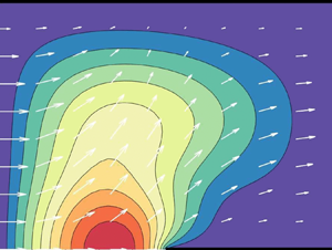
which provides a global accuracy test. As previously mentioned, technical difficulties arise where the ridge meets the meniscus. The presence of a stress singularity contaminates the numerical computations with errors. To improve convergence, singular derivatives must be removed from the triple contact line, and then reincorporated into the final solution – see Peyret (Reference Peyret2013). Also, see an earlier work by Woods (Reference Woods1953) which was motivated by the so-called Motz problem (Motz Reference Motz1947). The algorithm for the background flow has been tested extensively with the SHSP paradigm results of Game et al. (Reference Game, Hodes, Kirk and Papageorgiou2018), and agreement is excellent. For completeness, two of the streamwise velocity profiles generated are given in figure 2, for typical SHSC and SHSP flows – see figures 2(a) and 2(b), respectively. For more details on such flows and their properties, see the references provided in § 1.

Figure 2. Contours of constant streamwise velocity, for: (a) SHSC flow, and (b) SHSP flow, where  $h=1$ and
  $\delta =0.5$. The thick dark lines represent the solid boundaries of the channel.
The introduction of SHSs are known to result in reductions in viscous drag (Ou & Rothstein Reference Ou and Rothstein2005), due to higher velocities which are attained over the suspended gas region. Our objective is to study the stability of such flows in a parameter regime where drag reduction is optimised for applications. We characterise the drag reduction by computing the normalised flow rates  $\hat {Q}_c={Q_c}/{\tilde {Q}_c}$ and
  $\hat {Q}_p={Q_p}/{\tilde {Q}_p}$, where the flow rates
  $Q_c$ and
  $Q_p$ are calculated via (3.8) for each base state; similarly,
  $\tilde {Q}_c=h$ and
  $\tilde {Q}_p=h^3/6$ are the flow rates for smooth boundary Couette and PPFs per unit width. The normalised flow rates,
  $\hat {Q}_c$ and
  $\hat {Q}_p$, are plotted in figure 3 against the half-channel height
  $h$, and for a range of slip fractions
  $\delta$. The largest values are attained for small
  $h$ and large
  $\delta$ as expected. Physically, however, we must be careful to ensure that a Cassie–Baxter state can be maintained in this limiting regime – see Cassie & Baxter (Reference Cassie and Baxter1944). Nonetheless, via arguments given within Kirk et al. (Reference Kirk, Hodes and Papageorgiou2017), it may be deduced that the area of the parameter space considered here lies well within this range. Here, the authors relate their solutions to the molecular dynamic simulations of Cottin-Bizonne et al. (Reference Cottin-Bizonne, Barentin, Charlaix, Bocquet and Barrat2004), where it can be deduced that
  $h\ll 1$ for the surface to become wetted. One observes greater improvements for the SHSP flow in figure 3(b), which is as to be expected due to the uniform forcing throughout the interior of the domain. The qualitative development concerning the channel height is similar for the two configurations. We also note that as
  $h\rightarrow \infty$ then
  $\hat {Q}_c$ and
  $\hat {Q}_p \rightarrow 1$, so that the SHS has little effect on the flow rate unless
  $\delta$ is close to unity. Finally, these results are supported by the experiments of Ou et al. (Reference Ou, Perot and Rothstein2004), where the same dependencies for
  $\hat {Q}_p$ are reported. These experiments are discussed next. At this stage, we consider the situation where the meniscus is curved, in order to evaluate where our flat interface approximation is valid. Using the code developed in Game et al. (Reference Game, Hodes, Kirk and Papageorgiou2018), we evaluate the flow rate and Nusselt number from
  $\delta \in [0.25,0.75]$,
  $\varphi = [-45^\circ,45^\circ$] and
  $h\in [1,20]$. For
  $h>2$, then the maximum variation away from the
  $\varphi =0^\circ$ case is approximately 5 %. For
  $h<2$, it becomes important to take into account meniscus curvature, however, we retain these results to compare with the experiments in Ou et al. (Reference Ou, Perot and Rothstein2004).

Figure 3. The normalised flow rate for: (a) SHSC, and (b) SHSP problems.
3.4. Comparison with experiment
Our theoretical study enables the evaluation of the stability of a wide range of basic states at different Reynolds numbers. Due to the large Reynolds numbers required for linear instability of PPF (Couette flow is stable at all  $\textit {Re}$), we carry out numerical experiments at such large values for comparison and also to underpin future large Reynolds number analyses. It should be noted, however, that other nonlinear mechanisms such as vortex–wave interactions (Waleffe Reference Waleffe1997; Hall & Sherwyn Reference Hall and Sherwyn2010), can induce transition at lower Reynolds numbers than those predicted by linear theory, and such aspects for SHSC flows are left for future studies.
Our main interest here is to discuss physical experiments in SH channels that operate in parameter regimes that support instabilities in the present study. We choose to describe the experiments in Ou et al. (Reference Ou, Perot and Rothstein2004); Ou & Rothstein (Reference Ou and Rothstein2005), that were the original motivation for the present work. These researchers considered (among other surface structuring) longitudinal ridges as in figure 1. In the comparisons that follow we will use our notation adopted to that of the experiments. The width  $w^*$ of the channels in the experiments is finite and selected to be
  $20$ times the channel height
  $h^*$, i.e.
  $w^*=20 h^*$, justifying our ridge periodicity assumption away from the walls. Ou et al. (Reference Ou, Perot and Rothstein2004) and Ou & Rothstein (Reference Ou and Rothstein2005) report flow rates
  $Q^*$ between
  $0.03$ and
  $115\ \textrm {mm}^3\ \textrm {s}^{-1}$ and channel thicknesses
  $76\ \mathrm {\mu }\textrm {m}< h^*<254\ \mathrm {\mu }\textrm {m}$. Results for a range of solid ridge sizes separated by gas cavities of different widths are reported. The Reynolds number in the experiments is defined by
  $\textit {Re}_{ou}= U^*_{ou} D^*/\nu ^*$, where
  $U^*_{ou}=Q^*/A^*$ is the average velocity,
  $A^*=w^*h^*=20 h^{*2}$ is the channel cross-sectional area and
  $D^* = 4A^*/P^*$ is the hydraulic diameter where
  $P^*=2(w^*+h^*)=42h^*$ is the channel perimeter. Expressing our Reynolds number in terms of
  $\textit {Re}_{ou}$ gives
  $\textit {Re}=U^* d^*/\nu ^*=(d^*/D^*)\textit {Re}_{ou}=(21 d^*)(40 h^*)\textit {Re}_{ou}$. Writing
  $\textit {Re}_{ou}$ in terms of
  $Q^*$ and
  $h^*$ for the experiments provides
  $\textit {Re}_{ou}= (2 Q^*)/ (21\nu ^* h^*)$. Using
  $\rho ^*=1\ \textrm {g}\ (\textrm {cm}^{-3}$),
  $\nu ^*=10^{-6}\ \textrm {m}^{2}\ \textrm {s}^{-1}$ for water along with the flow rate and channel thickness ranges gives
  $0 \lesssim \textit {Re}_{ou} \lesssim 144$. Most experiments are performed for three sets of ridge pitch and slip fractions
  $(d^*, a^*)$; in terms of our variables these are
  $(30\ \mathrm {\mu }\textrm {m}, 15\ \mathrm {\mu }\textrm {m})$,
  $(45\ \mathrm {\mu }\textrm {m}, 15\ \mathrm {\mu }\textrm {m})$,
  $(20\ \mathrm {\mu }\textrm {m}, 10\ \mathrm {\mu }\textrm {m})$ which give slip fractions
  $\delta =1/2$ and
  $\delta = 1/3$. In addition, the dimensionless channel heights
  $h=h^*/d^*$ in the experiments have a range
  $1.7 \lesssim h \lesssim 12.7$ thus placing our computations in the experimental realm. Finally, considering values for
  $\textit {Re}$, we see that for the experiments this can be as large as
  $\textit {Re}\approx 47$ which is of the same order of magnitude for the critical Reynolds numbers computed in § 6.4 for pressure-driven flows over SHSs. Furthermore, it is commonly stated that the Reynolds number should be less than
  $1000$ for the flow to be laminar (where this definition is based on the half-channel height). This means that the range
  $\textit {Re} \in [0,311]$ requires consideration for the subset of slip fractions found in these experiments. However, in order to connect with the plane flow results that are considerably more stable, a larger interval is necessary. As
  $\delta \rightarrow 0$ and for
  $h = 2$, say, then the critical Reynolds number
  $\textit {Re}_c \approx 5772$ of plane Poiseuille flow is recovered. As a compromise between these two regimes, in § 6.3, we will take
  $\textit {Re} \in [0,5000]$.
We also note, for completeness, the experiments of Daniello et al. (Reference Daniello, Waterhouse and Rothstein2009) that are also of interest to the present study. Those authors considered drag reduction using SHSs as in our study but for much larger channel heights from the earlier studies of Ou et al. (Reference Ou, Perot and Rothstein2004) and Ou & Rothstein (Reference Ou and Rothstein2005). The ridge pitch was still of the order of  $30$ to
  $60\ \mathrm {\mu }\textrm {m}$ but the channel height
  $h^*$ was between 5.5 and 7.9 mm, thus giving dimensionless heights
  $h$ of approximately
  $100$. A particular comparison is made later where we compute with parameters directly taken from the experiment and find a reasonable prediction of transition. Note that, in the laminar regime, Daniello et al. (Reference Daniello, Waterhouse and Rothstein2009) find little effect of the SH surfaces. However, dramatic gains in drag reduction are found in the turbulent regime; due to an interaction of the SH scales with the turbulent wall layer.
4. Linear stability
4.1. Linearised stability equations
We are mostly concerned with shear instability modes. Hence, in our linearisation we assume that the liquid–gas interface remains fixed, and interfacial modes are excluded from the present study. We introduce perturbations of amplitude  $\epsilon$ around the basic states calculated in § 3, by writing
 \begin{equation} \begin{pmatrix}
u(\boldsymbol{r};t) \\ v(\boldsymbol{r};t) \\
w(\boldsymbol{r};t) \\ p(\boldsymbol{r};t)\end{pmatrix} = \begin{pmatrix} U(y,z) \\ 0 \\ 0
\\ \mathcal{B}x \\ \end{pmatrix} + \epsilon \begin{pmatrix}
\tilde{u}(y,z) \\ \tilde{v}(y,z) \\ \tilde{w}(y,z) \\
\tilde{p}(y,z) \\ \end{pmatrix}\exp(\textrm{i}(kx-\omega
t)) + \text{c.c.}, \end{equation}
\begin{equation} \begin{pmatrix}
u(\boldsymbol{r};t) \\ v(\boldsymbol{r};t) \\
w(\boldsymbol{r};t) \\ p(\boldsymbol{r};t)\end{pmatrix} = \begin{pmatrix} U(y,z) \\ 0 \\ 0
\\ \mathcal{B}x \\ \end{pmatrix} + \epsilon \begin{pmatrix}
\tilde{u}(y,z) \\ \tilde{v}(y,z) \\ \tilde{w}(y,z) \\
\tilde{p}(y,z) \\ \end{pmatrix}\exp(\textrm{i}(kx-\omega
t)) + \text{c.c.}, \end{equation}
where  $k$ is the real streamwise wavenumber,
  $\omega$ is the complex frequency and
  $\text {c.c.}$ denotes the complex conjugate. The constant
  $\mathcal {B}=0$ and
  $-2/\textit {Re}$, for the lid- and pressure-driven flows, respectively. Substituting (4.1) into (2.1)–(2.2) and linearising in
  $\epsilon$, gives the disturbance equations
 $$\begin{gather} \textrm{i}k \tilde{u} + \frac{\partial \tilde{v}}{\partial y} + \frac{\partial \tilde{w}}{\partial z} = 0, \end{gather}$$
 $$\begin{gather}\textrm{i}k (U-c)\tilde{u} + \frac{\partial U}{\partial y} \tilde{v} + \frac{\partial U}{\partial z} \tilde{w} ={-} \textrm{i} k \tilde{p} + \frac{1}{\textit{Re}}\left({-}k^2 \tilde{u}+\frac{\partial^2 \tilde{u}}{\partial y^2}+\frac{\partial^2 \tilde{u}}{\partial z^2}\right), \end{gather}$$
 $$\begin{gather}\textrm{i}k(U-c)\tilde{v} ={-} \frac{\partial \tilde{p}}{\partial y} + \frac{1}{\textit{Re}}\left({-}k^2 \tilde{v}+\frac{\partial^2 \tilde{v}}{\partial y^2}+\frac{\partial^2 \tilde{v}}{\partial z^2}\right), \end{gather}$$
and
 \begin{equation} \textrm{i}k(U-c)\tilde{w} ={-} \frac{\partial \tilde{p}}{\partial z} + \frac{1}{\textit{Re}}\left({-}k^2 \tilde{w}+\frac{\partial^2 \tilde{w}}{\partial y^2}+\frac{\partial^2 \tilde{w}}{\partial z^2}\right). \end{equation}
It is possible to reduce this set of equations from four to two, for the normal and spanwise variables – see Tatsumi & Yoshimura (Reference Tatsumi and Yoshimura1990). However, the primitive variable formulation was chosen here as the boundary conditions and singularity removal methodology are simpler to implement. Taking  $\textit {Re}\to \infty$ and eliminating:
  $\tilde {u}$,
  $\tilde {v}$ and
  $\tilde {w}$ in favour of
  $\tilde {p}$, we arrive at the two-dimensional Rayleigh equation
 \begin{equation} \frac{\partial^2 \tilde{p} }{\partial y^2} + \frac{\partial^2 \tilde{p} }{\partial z^2} - \frac{2 }{U-c}\frac{\partial U}{\partial y} \frac{\partial \tilde{p}}{\partial y} - \frac{2}{U-c}\frac{\partial U}{\partial z}\frac{\partial \tilde{p}}{\partial z} - k^2 \tilde{p} = 0. \end{equation}
Regarding general viscous boundary conditions, the bottom boundary of the SH channel consists of two parts requiring different constraints. Along the liquid–solid part we apply no slip in the velocity perturbations, so that
 \begin{equation} \tilde{u}(0,z_{ns}) = \tilde{v}(0,z_{ns}) = \tilde{w}(0,z_{ns}) = 0. \end{equation}
Then, similar to § 3, assuming no-shear stress and no-penetration conditions along the meniscus (Game et al. Reference Game, Hodes, Keaveny and Papageorgiou2017), we obtain
 \begin{equation} \frac{\partial \tilde{u}}{\partial y}(0,z_{s}) = \tilde{v}(0,z_{s}) = \frac{\partial \tilde{w}}{\partial y}(0,z_{s}) = 0. \end{equation}
Considering (4.4) with  $\textit {Re}\gg 1$, and noting that
  $\tilde {v}(0,z)=0$ on the boundary (for both liquid–gas and liquid–solid contact lines), yields
 \begin{equation} \frac{\partial \tilde{p}}{\partial y}(0,z)=0, \end{equation}
to be used in solving (4.6). At the top solid boundary we need to impose the no-slip condition to all velocity variables. That is
 \begin{equation} \tilde{u}(h,z) = \tilde{v}(h,z) = \tilde{w}(h,z) = 0, \end{equation}
for the viscous problem (4.2)–(4.5), and
 \begin{equation} \frac{\partial \tilde{p}}{\partial y}(h,z)=0, \end{equation}
in the inviscid problem (4.6). Due to spanwise periodicity across the ridges, both symmetric and anti-symmetric modes in  $z$ must be considered (Tatsumi & Yoshimura Reference Tatsumi and Yoshimura1990). A summary of the configurations and conditions on all variables are given in table 1, where we identify symmetric modes by the label 1 and anti-symmetric ones by 2.
Table 1. A summary of the different mode types considered within this work: a symmetric mode, which requires Dirichlet boundary conditions at  $z=0$ and
  $z=1$, or an anti-symmetric mode, which requires Neumann ones instead. The notation ‘s’ (‘as’) is used to mean symmetry (anti-symmetry) in the appropriate coordinate direction and, lastly, ‘-’ means that no simplifications could be made in this case.

4.2. A bi-global GEVP
Upon rearranging (4.2)–(4.5) or (4.6), we arrive at what is known as a continuous bi-global GEVP – see Theofilis et al. (Reference Theofilis, Duck and Owen2004). Solving this system to find non-trivial eigenvalues and eigenvectors provides a dispersion relation  $f(k,\omega ; \delta,h,\textit {Re})=0$, say. We adopt a temporal instability framework by fixing the wavenumber
  $k$ to be real and calculating complex
  $\omega =\omega _r+\textrm {i}\omega _i$ (instability follows if
  $\omega _i>0$). For the inviscid problem, we are interested in the modes with the largest growth rates, and hence neutral stability is not considered in detail. At neutral conditions, the dynamics inside critical layers is important and is left for future work (Hall & Horseman Reference Hall and Horseman1991).
4.3. Singularity removal
As mentioned earlier, the stress singularities at triple contact points ( $z=\delta$ in our domain) are removed before carrying out computations. Details are provided in Appendix A, where we describe the technique for the basic state (following Game et al. Reference Game, Hodes, Keaveny and Papageorgiou2017, Reference Game, Hodes, Kirk and Papageorgiou2018). We then modify it for the viscous and inviscid stability equations (4.2)–(4.5) and (4.6), respectively, that inherit their singularities through
  $U$ and its spatial derivatives.
We begin with the background flow and remove as many as two singularities as described in Appendix A.2. We write, for example,  $U = B^s_1 U^{s}_1 + \bar {U}$, where the singular part is
  $U^{s}_1=r^{1/2}\sin (\theta /2)$ in a local polar coordinate system (see (A3)),
  $B^s_1$ is its strength and
  $\bar {U}$ is the regular part (Peyret Reference Peyret2013). The unknown strength
  $B^s_1$ was determined by imposing the following first derivative regularity condition on
  $\bar {U}$:
 \begin{equation} \mathcal{R}^b \bar{U} \equiv \frac{\partial \bar{U}}{\partial z}(0,\delta ) = 0. \end{equation}
The choice (4.12) is not unique; indeed, a derivative in any direction and of any value could have been chosen (Game et al. Reference Game, Hodes, Kirk and Papageorgiou2018). However, the composite solution  $U$ is unique. The governing equations, (3.1) or (3.5), can be written in matrix form as
 \begin{equation} \begin{pmatrix}
\mathcal{P} & \mathcal{P} U^s_1 \\ \mathcal{R}^b & 0\end{pmatrix} \begin{pmatrix} \bar{U} \\ B_1^s \\
\end{pmatrix}= \begin{pmatrix} d \\ 0 \\ \end{pmatrix}, \end{equation}
\begin{equation} \begin{pmatrix}
\mathcal{P} & \mathcal{P} U^s_1 \\ \mathcal{R}^b & 0\end{pmatrix} \begin{pmatrix} \bar{U} \\ B_1^s \\
\end{pmatrix}= \begin{pmatrix} d \\ 0 \\ \end{pmatrix}, \end{equation}
where  $\mathcal {P}=\partial ^2/\partial y^2+\partial ^2/\partial z^2$, and
  $\mathcal {R}^b$ denotes the derivative operator evaluated at the singular point (defined in (4.12)). In addition,
  $d=-2$ for a pressure-driven flow, and
  $d=0$ for the lid-driven case. Multiplying (4.6) by
  $U-c$ and defining the differential operators
  $\mathcal {A}$ and
  $\mathcal {B}$, casts the Rayleigh equation into
 \begin{align} \mathcal{A} \tilde{p} &\equiv \left\{U \left(\frac{\partial^2 }{\partial y^2} + \frac{\partial^2 }{\partial z^2} - k^2\right)-2\frac{\partial U}{\partial y}\frac{\partial}{\partial y} - 2\frac{\partial U}{\partial z}\frac{\partial}{\partial z}\right\}\tilde{p} \nonumber\\ &= c \left\{\frac{\partial^2 }{\partial y^2} + \frac{\partial^2 }{\partial z^2} - k^2\right\}\tilde{p} \equiv c \mathcal{B} \tilde{p}. \end{align}
Then, as the pressure eigenmode has first-order derivatives that are regular (see Appendix A.3), this is all that is required for the inviscid eigenvalue problem (EVP). For the viscous problem, we also rearrange our system into a GEVP form by writing
 $$\begin{gather} \textrm{i}k \tilde{u} + \frac{\partial \tilde{v}}{\partial y} + \frac{\partial \tilde{w}}{\partial z} = 0, \end{gather}$$
 $$\begin{gather}\mathcal{S} \tilde{u} + \frac{\partial U}{\partial y} \tilde{v} + \frac{\partial U}{\partial z}\tilde{w} + \textrm{i} k \tilde{p} = \textrm{i} k \tilde{u}\,c, \end{gather}$$
 $$\begin{gather}\mathcal{S} \tilde{v} + \frac{\partial \tilde{p}}{\partial y} = \textrm{i} k \tilde{v}\,c, \end{gather}$$
and
 \begin{equation} \mathcal{S} \tilde{w} + \frac{\partial \tilde{p}}{\partial z} = \textrm{i} k \tilde{w}\,c, \end{equation}
where the operator  $\mathcal {S} \equiv \textrm {i} k U + (1/\textit {Re})(-k^2 + \partial ^2/\partial y^2 + \partial ^2/\partial z^2)$. From Appendix A.4, we know that the streamwise velocity field decomposes as
  $\tilde {u} = U^s_1 \tilde {u}^s_1 + \bar {u}$, the wall-normal velocity field takes the form
  $\tilde {v} = \bar {v}$, the spanwise velocity field becomes
  $\tilde {w} = \bar {w}$ and the pressure field decomposes as
  $\tilde {p} = P^s_1 \tilde {p}^s_1 + \bar {p}$. The regularity conditions for the basic state variables that require singularity removal read
 \begin{equation} \mathcal{R}^b \bar{u}= \mathcal{R}^b\bar{p} = 0. \end{equation}
Defining the regularised basic state and singular coefficient vectors by  $\bar {\boldsymbol {q}}\equiv (\bar {u}, \bar {v}, \bar {w}, \bar {p})^\textrm {T}$ and
  $\boldsymbol {Q}^s \equiv (U^s_1, P^s_1)^\textrm {T}$ respectively, we arrive at the following GEVP:
 \begin{equation} \begin{pmatrix} \boldsymbol{\mathcal{E}} & \boldsymbol{\mathcal{E}}^s \\ \boldsymbol{\mathcal{R}}^v & \boldsymbol{\mathcal{O}} \end{pmatrix} \begin{pmatrix} \boldsymbol{\bar{q}} \\ \boldsymbol{Q}^s \end{pmatrix}= c \begin{pmatrix} \boldsymbol{\mathcal{F}} & \boldsymbol{\mathcal{F}}^s \\ \boldsymbol{\mathcal{O}} & \boldsymbol{\mathcal{O}} \end{pmatrix} \begin{pmatrix} \boldsymbol{\bar{q}} \\ \boldsymbol{Q}^s \end{pmatrix}. \end{equation}
The sub-matrices are referred to as the regular matrices
 \begin{equation} \boldsymbol{\mathcal{E}} \equiv \begin{pmatrix} \textrm{i}k & \partial_y & \partial_z & 0 \\ \mathcal{S} & U_y & U_z & \textrm{i}k \\ 0 & \mathcal{S} & 0 & \partial_y \\ 0 & 0 & \mathcal{S} & \partial_z \\ \end{pmatrix} \quad \text{and} \quad \boldsymbol{\mathcal{F}} \equiv \begin{pmatrix} 0 & 0 & 0 & 0 \\ \textrm{i} k & 0 & 0 & 0 \\ 0 & \textrm{i} k & 0 & 0 \\ 0 & 0 & \textrm{i} k & 0 \\ \end{pmatrix}, \end{equation}
the singular matrices
 \begin{equation}
\boldsymbol{\mathcal{E}}^s \equiv \begin{pmatrix}
\textrm{i}k \tilde{u}_1^s & 0 \\ \mathcal{S} \tilde{u}_1^s
& \textrm{i}k \tilde{p}_1^s \\ 0 & \partial_y \tilde{p}_1^s
\\ 0 & \partial_z \tilde{p}_1^s \end{pmatrix} \quad
\text{and} \quad \boldsymbol{\mathcal{F}}^s \equiv
\begin{pmatrix} 0 & 0 \\ \textrm{i} k \tilde{u}_1^s & 0 \\
0 & 0 \\ 0 & 0
\end{pmatrix},
\end{equation}
\begin{equation}
\boldsymbol{\mathcal{E}}^s \equiv \begin{pmatrix}
\textrm{i}k \tilde{u}_1^s & 0 \\ \mathcal{S} \tilde{u}_1^s
& \textrm{i}k \tilde{p}_1^s \\ 0 & \partial_y \tilde{p}_1^s
\\ 0 & \partial_z \tilde{p}_1^s \end{pmatrix} \quad
\text{and} \quad \boldsymbol{\mathcal{F}}^s \equiv
\begin{pmatrix} 0 & 0 \\ \textrm{i} k \tilde{u}_1^s & 0 \\
0 & 0 \\ 0 & 0
\end{pmatrix},
\end{equation}
and a regularity matrix
 \begin{equation} \boldsymbol{\mathcal{R}}^v \equiv \begin{pmatrix} \mathcal{R}^b & 0 & 0 & 0 \\ 0 & 0 & 0 & \mathcal{R}^b\end{pmatrix}. \end{equation}
The systems (4.13), (4.14) and (4.20) derived above, represent the governing equations for the background flow, inviscid, and viscous EVPs respectively (with singular derivatives removed up to  $O(r)$).
5. Numerical procedure and algorithmic considerations
5.1. Domain decomposition
We begin by decomposing the domain into two rectangular regions separated by a line perpendicular to the SHS and originating from the triple contact point – see figure 4. These are then mapped to  $\mathcal {D}_n \equiv \{\xi \in [-1,1]\}\times \{\eta \in [-1,1]\}$, using the transformations
 \begin{equation} (\xi_1,\xi_2,\eta) = \left(\frac{2z_s}{\delta}-1,\frac{2(z_{ns}-\delta)}{1-\delta}-1,\frac{2y}{h} -1\right), \end{equation}
so that standard Chebyshev collocation methods can be used in each region. We introduce discrete points inside the domain, using  $N=(N_\xi +1)(N_\eta +1)$ nodes at the locations
 \begin{equation} (\xi_i,\eta_j) = \left(\cos\left(\textrm{i}{\rm \pi}/N_\xi\right), \cos\left(j{\rm \pi}/N_\eta\right)\right), \end{equation}
where  $i=0,1,\ldots,N_\xi$ and
  $j=0,1,\ldots,N_\eta$. The lateral and horizontal domain boundaries are given by
  $i=0$ and
  $N_\xi$, and
  $j=0$ and
  $N_\eta$, respectively. Additional continuity conditions are imposed at the common sub-domain boundaries
 \begin{equation} \boldsymbol{R}_1=\boldsymbol{R}_2 \quad \text{and} \quad \frac{\partial \boldsymbol{R}_1}{\partial z_1}=\frac{\partial \boldsymbol{R}_2}{\partial z_2} \quad \text{for} \ \boldsymbol{R}_n\equiv(\bar{U}, \bar{\boldsymbol{q}}), \end{equation}
where  $n=1,2$ represents the evaluation of a given variable
  $\boldsymbol {R}$ in a particular domain, and
  $\bar {\boldsymbol {q}}$ is as defined in § 4.3.

Figure 4. A schematic illustrating the way in which the domain is decomposed into two sub-domains: (a) depicts the whole domain, (b) domain 1 and (c) domain 2. These are then transformed to  $\mathcal {D}_n$, such that Chebyshev collocation techniques can be used.
Evaluating (4.13) in each domain and incorporating (5.3), (4.13) becomes
 \begin{equation} \begin{pmatrix}
\boldsymbol{\mathsf{P}}_1 &
\boldsymbol{\mathsf{M}}_{12} &
\boldsymbol{\mathsf{P}}_1\boldsymbol{U}_{1}^s +
\boldsymbol{\mathsf{M}}_{12}\boldsymbol{U}_{2}^s \\
\boldsymbol{\mathsf{M}}_{21} &
\boldsymbol{\mathsf{P}}_{2} &
\boldsymbol{\mathsf{M}}_{21} \boldsymbol{U}_{1}^s +
\boldsymbol{\mathsf{P}} _2\boldsymbol{U}_{2}^s \\
\boldsymbol{\mathsf{R}}^b_1 &
\boldsymbol{\mathsf{R}}_2^b & 0 \end{pmatrix}
\begin{pmatrix} \overline{\boldsymbol{U}}_1 \\
\overline{\boldsymbol{U}}_2 \\ B_1^s \end{pmatrix}=
\begin{pmatrix} \boldsymbol{d}_1 \\ \boldsymbol{d}_2 \\ 0
\end{pmatrix}. \end{equation}
\begin{equation} \begin{pmatrix}
\boldsymbol{\mathsf{P}}_1 &
\boldsymbol{\mathsf{M}}_{12} &
\boldsymbol{\mathsf{P}}_1\boldsymbol{U}_{1}^s +
\boldsymbol{\mathsf{M}}_{12}\boldsymbol{U}_{2}^s \\
\boldsymbol{\mathsf{M}}_{21} &
\boldsymbol{\mathsf{P}}_{2} &
\boldsymbol{\mathsf{M}}_{21} \boldsymbol{U}_{1}^s +
\boldsymbol{\mathsf{P}} _2\boldsymbol{U}_{2}^s \\
\boldsymbol{\mathsf{R}}^b_1 &
\boldsymbol{\mathsf{R}}_2^b & 0 \end{pmatrix}
\begin{pmatrix} \overline{\boldsymbol{U}}_1 \\
\overline{\boldsymbol{U}}_2 \\ B_1^s \end{pmatrix}=
\begin{pmatrix} \boldsymbol{d}_1 \\ \boldsymbol{d}_2 \\ 0
\end{pmatrix}. \end{equation}
The contributions  $\boldsymbol{\mathsf{M}}_{12}$ and
  $\boldsymbol{\mathsf{M}}_{21}$, apply the discretised matching conditions from (5.3). The inviscid stability equation (4.14) becomes
 \begin{equation} \begin{pmatrix} \boldsymbol{\mathsf{A}}_1 & \boldsymbol{\mathsf{M}}_{12} \\ \boldsymbol{\mathsf{M}}_{21} & \boldsymbol{\mathsf{A}}_{2} \end{pmatrix} \begin{pmatrix} \bar{\boldsymbol{p}}_1 \\ \bar{\boldsymbol{p}}_2 \end{pmatrix} =c \begin{pmatrix} \boldsymbol{\mathsf{B}}_1 & \boldsymbol{\mathsf{M}}_{12} \\ \boldsymbol{\mathsf{M}}_{21} & \boldsymbol{\mathsf{B}}_{2} \end{pmatrix} \begin{pmatrix} \bar{\boldsymbol{p}}_1 \\ \bar{\boldsymbol{p}}_2 \end{pmatrix}. \end{equation}
All matrices  $\boldsymbol{\mathsf{A}}_n,\boldsymbol{\mathsf{B}}_n,\boldsymbol{\mathsf{P}}_n,\boldsymbol{\mathsf{M}}_{12}$ and
  $\boldsymbol{\mathsf{M}}_{21}$ for
  $n=1,2$, have dimension
  $N\times N$ and the elements
  $\boldsymbol{\mathsf{R}}^b_n$ for
  $n=1,2$, which apply the regularity condition to the less singular function in the bottom row of (5.4), are of size
  $1\times N$. Conversely, the elements in the new column that apply the governing equation, matching and boundary conditions, to the leading-order singular expression are
  $N\times 1$. Lastly, taking (4.15)–(4.19), discretising and incorporating of the boundary conditions, we arrive at
 \begin{equation} \begin{pmatrix}
\boldsymbol{\mathsf{E}}_1 &
\boldsymbol{\mathsf{M}}_{12} &
\boldsymbol{\mathsf{E}}_1^s +
\boldsymbol{\mathsf{M}}_{12}^s \\
\boldsymbol{\mathsf{M}}_{21} &
\boldsymbol{\mathsf{E}}_{2} &
\boldsymbol{\mathsf{M}}_{21}^s +
\boldsymbol{\mathsf{E}}_{2}^s \\
\boldsymbol{\mathsf{R}}^v_1 &
\boldsymbol{\mathsf{R}}^v_2 &
\boldsymbol{\mathsf{O}} \end{pmatrix}
\begin{pmatrix} \bar{\boldsymbol{q}}_1 \\
\bar{\boldsymbol{q}}_2 \\ \boldsymbol{Q}^s \end{pmatrix}
=c \begin{pmatrix} \boldsymbol{\mathsf{F}}_1 &
\boldsymbol{\mathsf{M}}_{12} &
\boldsymbol{\mathsf{F}}^s_1 +
\boldsymbol{\mathsf{M}}_{12}^s \\
\boldsymbol{\mathsf{M}}_{21} &
\boldsymbol{\mathsf{F}}_{2} &
\boldsymbol{\mathsf{M}}_{21}^s +
\boldsymbol{\mathsf{F}}^s_{2} \\
\boldsymbol{\mathsf{O}} & \boldsymbol{\mathsf{O}}
& \boldsymbol{\mathsf{O}} \end{pmatrix}
\begin{pmatrix} \bar{\boldsymbol{q}}_1 \\
\bar{\boldsymbol{q}}_2 \\ \boldsymbol{Q}^s \end{pmatrix}.
\end{equation}
\begin{equation} \begin{pmatrix}
\boldsymbol{\mathsf{E}}_1 &
\boldsymbol{\mathsf{M}}_{12} &
\boldsymbol{\mathsf{E}}_1^s +
\boldsymbol{\mathsf{M}}_{12}^s \\
\boldsymbol{\mathsf{M}}_{21} &
\boldsymbol{\mathsf{E}}_{2} &
\boldsymbol{\mathsf{M}}_{21}^s +
\boldsymbol{\mathsf{E}}_{2}^s \\
\boldsymbol{\mathsf{R}}^v_1 &
\boldsymbol{\mathsf{R}}^v_2 &
\boldsymbol{\mathsf{O}} \end{pmatrix}
\begin{pmatrix} \bar{\boldsymbol{q}}_1 \\
\bar{\boldsymbol{q}}_2 \\ \boldsymbol{Q}^s \end{pmatrix}
=c \begin{pmatrix} \boldsymbol{\mathsf{F}}_1 &
\boldsymbol{\mathsf{M}}_{12} &
\boldsymbol{\mathsf{F}}^s_1 +
\boldsymbol{\mathsf{M}}_{12}^s \\
\boldsymbol{\mathsf{M}}_{21} &
\boldsymbol{\mathsf{F}}_{2} &
\boldsymbol{\mathsf{M}}_{21}^s +
\boldsymbol{\mathsf{F}}^s_{2} \\
\boldsymbol{\mathsf{O}} & \boldsymbol{\mathsf{O}}
& \boldsymbol{\mathsf{O}} \end{pmatrix}
\begin{pmatrix} \bar{\boldsymbol{q}}_1 \\
\bar{\boldsymbol{q}}_2 \\ \boldsymbol{Q}^s \end{pmatrix}.
\end{equation}
Note that unlike the basic flow and inviscid stability problems, all matrices  $\boldsymbol{\mathsf{E}}_n,\boldsymbol{\mathsf{F}}_n,\boldsymbol{\mathsf{M}}_{12}$ and
  $\boldsymbol{\mathsf{M}}_{21}$ for
  $n=1,2$, are of size
  $4N \times 4N$. On the other hand, the elements in the new column added in (5.6) are of size
  $4N\times 2$, and they apply the field equation, matching and boundary conditions, to the first-order contributions in the singular expansions for streamwise velocity and pressure. Next,
  $\boldsymbol{\mathsf{R}}^v_n$ for
  $n=1,2$, are of size
  $2\times 4N$, and act as the discrete approximations to the regularity conditions. Finally,
  $\boldsymbol{\mathsf{O}}$ represents a zero matrix of an appropriate size.
5.2. Eigenvalue tracking algorithms
The above EVPs could be tackled by a QZ-algorithm to obtain the full spectrum. However, due to the size of the matrices (requiring memory and runtime requirements of  $O(N^2)$ and
  $O(N^3)$, respectively), this method was applied at low resolution, in order to provide us with an initial guess to the most unstable eigenvalue. An example of a simple local algorithm is the inverse iterations technique, implemented by Moradi & Floryan (Reference Moradi and Floryan2014). The final method to be discussed is the Krylov–Schur algorithm, which takes the form of eigs in MATLAB. This algorithm ordinarily has an advantage over the last two methods mentioned, in that it can be run without an initial guess. This is not the case in our problem, as one of the GEVP matrices is singular. This algorithm can be understood as a bridge between global and local techniques, and can also utilise sparsity, which is highly advantageous. In the results that follow, the Krylov–Schur algorithm was used to compute the most unstable eigenmodes presented. In Theofilis (Reference Theofilis2003), one may find a comparison between these two techniques.
6. Results and discussion
6.1. Validation of the numerical procedure
Before presenting our results we describe several validations of the code based on existing literature. The accuracy of the basic flow was evaluated by the flux calculations of § 3, which are in agreement with the work of Game et al. (Reference Game, Hodes, Keaveny and Papageorgiou2017, Reference Game, Hodes, Kirk and Papageorgiou2018). The spectral method and domain decomposition for the inviscid EVP has been validated by comparing with the work of Duck (Reference Duck2011), where good agreement with figure 4 from this reference has been established. Next, for the viscous EVP, the study of Theofilis et al. (Reference Theofilis, Duck and Owen2004) provides us with a paradigm to validate our algorithm. For the pressure-driven case an excellent agreement is achieved with the critical mode of duct aspect ratio  $A=5$, streamwise wavenumber
  $k=0.91$ and Reynolds number
  $\textit {Re}=10\,400$, with our converged eigenvalue given by
  $c=0.2323$. Similarly, in the lid-driven configuration, the stable mode
  $c=0.9033 - 0.0622\textrm {i}$ for
  $A=2$,
  $\textit {Re}=3800$ and
  $k=1$, was also recovered correct to four decimals. Note also that in all the validations above, an unnecessary domain decomposition was applied at some value
  $z=z^d$ in the interior of the domain. This is in anticipation of the stick-slip surface in SHS flows, and the agreement implies a further validation for the domain decomposition algorithm.
It remains to provide evidence that the removal of singular derivatives is working with the desired effect. We present results for the lid-driven viscous EVP with parameters  $h=1$,
  $k=1$,
  $\delta =0.5$ and
  $\textit {Re}=100$. Analogous to the streamwise flux which we used to monitor the convergence in (3.8), we define a perturbation norm
 \begin{equation} Q_{N_\eta}=\int_{z=0}^1\int_{y=0}^h{Re}[\tilde{u}+\tilde{v}+\tilde{w}+\tilde{p}]\,\text{d}z \,\text{d}y. \end{equation}
This allows one to estimate the residual error heuristically via the absolute value of the difference in successive fluxes  $|Q_{N_\eta }-Q_{N_\eta -2}|$, as the number
  $N_\eta$ of nodes in the wall-normal direction increases. The results are presented in figure 5, which includes numerical convergence calculations from a single domain discretisation, to two domains, to two domains with the leading-order singularity removed, and finally two domains with two leading-order singularities removed. In figure 5 we chose to fix
  $2N_\xi =N_\eta$, in order to keep the same number of nodes in either direction. Convergence is predicted for all cases and as expected, where the algebraic decay with
  $N_\eta$ is fastest for case (iv) that removes two leading-order singularities coupled with a domain decomposition. Figure 5(b) is a log–log plot, and the slope of the lines provide an estimate for the algebraic decay rate. In the stability results that follow, we chose to adopt case (iii). Namely, a domain decomposition with the leading-order singularity removed, to strike a balance between efficiency and accuracy. The same level of accuracy must be retained for the background flow. This is because convergence is limited to the lowest-order singularity left in the problem, and derivatives of this function force (4.2)–(4.5).

Figure 5. Convergence of the perturbation integral measure (6.1) for the SHSC problem, depicting: (a) the value of  $Q_{N_\eta }$, and (b) the difference between successive iterations, with parameters
  $h=1$,
  $k=1$,
  $\delta =0.5$ and
  $\textit {Re}=1000$. In (i) the circles correspond to a solution on one domain with no singularity removal, (ii) the pluses correspond to a solution on two domains and with no singularity removal, (iii) the asterisks correspond to a solution on two domains and with the leading-order singularity removed and (iv) the crosses correspond to a solution on two domains and with the two leading-order singularities removed.
Finally, we highlight the importance of our semi-analytical approach that combines singularity removal and domain decomposition in problems with irregular geometries (this is relevant to the curved meniscus SHSs also, that we study elsewhere). For example, with a resolution of around  $20$ nodes in the spanwise direction for a one domain spectral technique, an accuracy of one decimal place is achieved. On the other hand, with domain decomposition, two singularities removed and an equivalent resolution of approximately
  $10$ nodes per sub-domain in the spanwise direction, we can instead achieve accuracy greater than four decimal places which is a huge improvement. For problems which require higher resolution for convergence, e.g. large
  $h$ and
  $\textit {Re}$, similar comparable reductions in the required resolution are observed once the semi-analytical methodology is applied. It should be noted, however, that the improvements are not as dramatic for certain geometrical values (say either as
  $h\rightarrow 0$ or
  $\delta \rightarrow 0$), as these new singular limits instead dominate and corrupt the convergence rate (mathematically, two triple-point singularities come together and a separate asymptotic approximation becomes possible then – see Yariv & Schnitzer (Reference Yariv and Schnitzer2018) for such a study of a similar basic state problem). The simulations herein were carried out using maximum resolution of
  $N_\xi = 30$ nodes per sub-domain, which means an error of less than
  $10^{-8}$ when
  $h=1$ – see figure 5(b). When the height of the channel is greater this error increases (e.g. figures 7 and 10e,f), but is still small enough to ensure sufficient convergence in the growth rates presented herein.
6.2. The effect of SHSs, plane Couette and PPF
We begin by examining the results as the width of the gas cavity tends to zero, where the problem becomes invariant in the spanwise direction and tends to the flow between two parallel infinite plates. Our stability results should then tend to those of classical parallel channel shear flows. To simplify matters, we will only be considering those channels with a fixed aspect ratio having  $h=2$ (an appropriate scaling will generalise these results). Schmid & Henningson (Reference Schmid and Henningson2012) provide tables of the most unstable Orr–Sommerfeld and Squire modes for both plane Poiseuille and Couette flow. Considering first the pressure-driven configuration (as the transformation is more straight forward), the parallel background flow used within this reference is given by
  $U(y) = 1-y^2$ for
  $y \in [-1,1]$. As previously mentioned, this corresponds to taking
  $h=2$ in our geometry, with
  $k$ and
  $\textit {Re}$ unchanged (as the aspect ratio is the same in both configurations). For the Couette flow the domain remains the same, however, the background flow becomes
  $U(y) = y$ for
  $y \in [-1,1]$. This again means that there is no change in the governing length scale (and therefore the definitions of
  $k$ and
  $\textit {Re}$), but since our flow is now no longer uni-directional, an appropriate shift must be incorporated into the eigenvalue spectrum to make a meaningful comparison. By considering a flow driven by one moving plate, symmetry around
  $\textrm {Re}(c)=0$ in the resulting eigenvalue spectrum is lost.
The results in table 2 demonstrate the convergence of the most unstable mode to those arising in the parallel configuration, for discrete values of  $\delta$ close to zero. For the pressure- and lid-driven problems, the two modes with the largest growth rates are chosen. These correspond to parities given by SHSP2 then SHSP1, and SHSC2 then SHSC1, such that the anti-symmetry or symmetry of the streamwise velocity eigenfunction in the spanwise direction represents the difference between the Orr–Sommerfeld and Squire modes in each case (see table 1 for the definition of these modes). For modes SHSP2, SHSC2 and SHSC1, the progression from the parallel flow is gradual, with the final growth rate at
  $\delta =0.4$ correct to one significant figure. For a very small value of
  $\delta$ excellent agreement between the eigenvalues is achieved. On the other hand, the variation in slip fraction affects the SHSP1 mode much more drastically. As we will report later (see § 6.3), this is not important to the stability characteristics of the flow. This is because the growth rate of this mode is dominated by the SHSP2-mode, especially when
  $\delta$ is large and
  $h$ is small.
Table 2. A summary of the effects of the slip fraction on the plane flow modes, where the two eigenvalues with the largest growth rates are considered. The reference eigenvalues are taken from Schmid & Henningson (Reference Schmid and Henningson2012), with  $k=1$, and are denoted the plane flow (PF) eigenvalues.

To complement this analysis we also analyse the spectrum's dependence on  $\delta$ and the most unstable eigenmodes for
  $\delta =0.01$ in figure 6(a–c). In figure 6(a), one observes that, as the slip fraction increases, the P- and A-branches of the plane Poiseuille spectrum shift up and right, where they become unstable for
  $\delta =0.4$. We may examine both symmetric and antisymmetric streamwise velocity eigenmodes in figure 6, where both the wall (figure 6c) and centre modes (figure 6b) translate as the slip fraction is increased. The former and latter correspond to the Squire and Orr–Sommerfeld modes, respectively, from Schmid & Henningson (Reference Schmid and Henningson2012).

Figure 6. The spectrum and most unstable eigenmodes corresponding to plane Poiseuille flow, where (a) depicts  $100$ eigenvalues that are closest to the values in table 2 for different slip fractions (the large symbols denote the values presented in table 2), (b) is the velocity perturbation for the most unstable antisymmetric eigenmode and (c) is the velocity perturbation for the most unstable symmetric eigenmode for
  $\delta =0.01$.
6.3. Instability of lid-driven superhydrophobic channel flow
We begin by studying neutral curves to identify the regions of instability in terms of the key flow variables and geometrical parameters. We first consider the SHSC flow and search a relatively large region of the parameter space given by  $0\leqslant k\leqslant 3$ and
  $1\leqslant \textit {Re}\leqslant 5000$, considering both symmetric and non-symmetric modes of instability. We restrict
  $\textit {Re}\leqslant 5000$ since Reynolds numbers greater than this are unlikely to arise in micro-channel configurations (Ou et al. Reference Ou, Perot and Rothstein2004; Daniello et al. Reference Daniello, Waterhouse and Rothstein2009). In the former, the Reynolds number defined as
  $\textit {Re}_{ou}=U^*_{ou} D^* /\nu ^*$ (where
  $D^* = 4A^*/P^*$ is the hydraulic diameter,
  $A^*$ is the cross-sectional area and
  $P^*$ is the perimeter of the channel), is stated to be less than
  $1000$ such that the flows examined were observed to be laminar. Considering the differences in length and velocity scales, one has that
  $\textit {Re} = U^* d^* / \nu ^* \approx \textit {Re}_{ou} (d^* / h^*) (21/40) \in [0,311]$ explicitly require consideration; see § 3.4 for a more detailed discussion and derivation. We increase this Reynolds number interval to higher values in order to capture the full dynamics when
  $\delta \rightarrow 0$ (where the critical Reynolds numbers of PPF are recovered), allowing for theoretical predictions for parameters not covered in experiments.
The most unstable mode is found to be the SHSC2 mode, which is anti-symmetric in the spanwise direction, and in the remainder of this study, we concentrate on this mode alone. Our results indicate that the flow is stable in the limits  $k \rightarrow 0$ and
  $\infty$, implying that for a given Reynolds number, instability (if it exists) is restricted to a finite band of wavenumbers
  $k\in [k_{min},k_{max}]$, say. Furthermore, as
  $\textit {Re}\rightarrow \infty$ we have that
  $k_{min}, k_{max} \rightarrow 0$, such that the flow is inviscidly stable (this is discussed in greater detail in § 6.5). In figures 7(a)–7(e) we present the neutral curves and selected growth rates for different slip fractions ranging from
  $\delta =0.1$ to
  $0.9$, and channel heights ranging from
  $h=1$ to
  $10$. Figures 7(a), 7(c) and 7(d) show computed neutral curves in the
  $(k,\textit {Re})$-plane for channel heights
  $h=1, 2$ and
  $10$, respectively. In the accompanying figures 7(b), 7(d) and 7(e) we present growth rates at each slip fraction and fixed Reynolds number of
  $\textit {Re}=2500$,
  $1500$ and
  $1250$, respectively; this is identified by a dashed line in figures 7(a), 7(c) and 7(e).

Figure 7. Neutral curves for different channel heights in the SHSC problem, given by: (a)  $h=1$, (c)
  $h=2$ and (e)
  $h=10$, where the left-hand side of each line represents the stable, and the right-hand side the unstable, region of the
  $(k,\textit {Re})$-plane. Additionally included are the growth rates for different channel heights and Reynolds numbers, such that (b)
  $h=1$ and
  $\textit {Re}=2500$, (d)
  $h=2$ and
  $\textit {Re}=1500$ and (f)
  $h=10$ and
  $\textit {Re}=1250$.
It is observed that the most unstable configuration, in the sense of the one with the smallest critical Reynolds number, is where the greatest reductions in drag are observed for the basic flow. Namely, from § 3, this is in small channels with large exposed gas regions. For example, in figure 7(a), with  $h=1$ and
  $\delta =0.9$, the critical Reynolds number above which instability exists is
  $\textit {Re}_c \approx 200$. This then increases monotonically, as the channel height is increased, and the slip fraction is decreased. The value of the critical streamwise wavenumber, on the other hand, is seen to remain relatively constant in both of these limits, i.e.
  $k_c\approx 1$ for all
  $h$ and
  $\delta$. The maximum growth rates depicted in figures 7(b), 7(d) and 7(f) are seen to decrease with increasing
  $h$, and for the smaller channels having
  $h=1$ and
  $2$, a maximum is attained for
  $\delta =0.7$. The results also show clearly that a critical value of the slip fraction is necessary for this new instability mode to exist at the chosen range of Reynolds numbers. If we are below the critical value of
  $\delta$ (where physically, there is less slip than no slip exposed to the fluid), then we observe stability as in the plane flow or duct configuration (Theofilis et al. Reference Theofilis, Duck and Owen2004; Schmid & Henningson Reference Schmid and Henningson2012). Additional evidence is supplied by the neutral curves in figures 7(a), 7(c) and 7(e), where the separation between contours becomes larger for different slip fractions as
  $h$ is increased. Specifically, and for the range of Reynolds numbers considered, when
  $h=1$ no neutral curves (and hence no instability) could be found for
  $\delta \lesssim 0.3$ and
  $\textit {Re}\in [1,5000]$, when
  $h=2$ then
  $\delta \lesssim 0.4$ and
  $\textit {Re}\in [1,2000]$ and when
  $h=10$ then
  $\delta \lesssim 0.6$ and
  $\textit {Re}\in [1,2000]$. We can conclude, therefore, that given a
  $h$ and
  $\textit {Re}\in [1,5000]$, the flow is stable for
  $\delta <\delta _c(h,\textit {Re})$; where these values can be read off 9(a). The limit as
  $\textit {Re}\to \infty$ is considered in detail later.
Having identified unstable regions in parameter space, we turn to the examination of the structure of the disturbance field. The three components of velocity and pressure which form it, are two-dimensional functions of  $y$ and
  $z$, and depend on
  $\delta$,
  $h$,
$h$,  $\textit {Re}$ and
  $k$. We concentrate on the mode which becomes unstable first, and normalise it by its absolute maximum interior value, i.e.
  $\hat {\boldsymbol {q}} = |\tilde {\boldsymbol {q}}|/\max |\tilde {\boldsymbol {q}}|$, where
  $\tilde {\boldsymbol {q}}$ is defined in §5. In figures 8(a)–8(e) we present such eigenfunctions and in particular show the streamwise velocity field
  $\tilde {u}$ in the channel cross-sectional
  $(y,z)$-plane. We then superimpose the cross-plane velocity vector field
  $(\tilde {v},\tilde {w})$, by a collection of vectors that show its magnitude and direction. Hence, plots such as figure 8 (and figure 11 later on), allow us to view the full three-dimensional structure of the perturbation velocity field. The geometry corresponding to the different figures is characterised by
  $h=1$,
  $\delta =0.3-0.7$ for figures 8(a)–8(c),
  $h=2$,
  $\delta =0.5$ for figure 8(d) and
  $h=10$,
  $\delta =0.7$ for figure 8(e), with the values of the streamwise wavenumber and Reynolds number selected to attain near-critical instability. The critical disturbance forms a relatively high-velocity streak in the streamwise direction, which is located near the SHS and over the meniscus to the left of the solid region (as depicted in the figure). It can be seen to increase in size and translate when the channel height and slip fraction are increased respectively – see figures 8(a)–8(c). The cross-plane velocity field also affects a larger spanwise area and traverses from left to right where it meets the solid ridge. This encounter with the no-slip surface induces a vertical velocity and translation up and towards the top of the channel. Furthermore, the streamwise velocity is seen to decay rapidly for increasing
  $y$, so that in figure 8(e) where
  $h=10$, the majority of the channel is free from the disturbance. Increasing the slip fraction has the effect of translating this structure outwards in the positive wall-normal and spanwise directions, where there is less overhang into the area above the solid region. Finally, considering values around those which are critical, it is observed that an increase in the streamwise wavenumber concentrates the disturbance closer to the wall, whereas, a decrease diffuses it out. Variation in the Reynolds number around its critical value, on the other hand, have little to no qualitative effect.

Figure 8. Contours of constant streamwise velocity for the most unstable mode in the SHSC problem, with (a)  $h=1$,
  $\delta =0.3$ and
  $(k,\textit {Re})=(1.5,4000)$, (b)
  $h=1$,
  $\delta =0.5$ and
  $(k,\textit {Re})=(1.5,4000)$, (c)
  $h=1$,
  $\delta =0.7$ and
  $(k,\textit {Re})=(1.5,4000)$, (d)
  $h=2$,
  $\delta =0.5$ and
  $(k,\textit {Re})=(1,1500)$ and (e)
  $h=10$,
  $\delta =0.7$ and
  $(k,\textit {Re})=(1,1000)$. Here, the arrows represent the cross-plane velocity field such that all values are normalised, and lastly, the thick lines on the boundary represent the solid wall regions.
Having given details of the underlying instabilities and corresponding eigenfunction structures, we summarise our computational findings by constructing the variation of the critical Reynolds number  $\textit {Re}_c$ with the channel height and slip fraction. Such data could be of considerable use in practical design and operation of SH channel flows, and we emphasise that little theoretical attention has been given to instabilities in such flows. The results are given in figure 9(a,b) for the variation of
  $\textit {Re}_c$ and the corresponding instability phase velocity, respectively. As the channel height is increased it is observed that the value of
  $\textit {Re}_c$ also increases. This because we are considering a fixed lid velocity and therefore shear rate (i.e.
  $U(h,z)=2$), whose value decreases with increasing
  $h$. Furthermore, as the slip fraction is reduced from
  $\delta =0.9$ to
  $0.3$, the critical Reynolds number also increases monotonically. Indeed the increase of
  $\textit {Re}_c$ with a decrease in
  $\delta$ is quite dramatic; for example, fixing
  $h=1$ and decreasing
  $\delta$ from
  $0.9$ to
  $0.7$ results in a doubling of
  $\textit {Re}_c$ to approximately
  $500$. While a further decrease to
  $\delta =0.4$ yields
  $\textit {Re}_c\approx 2250$, i.e. a tenfold increase. Note that such large increases in
  $\textit {Re}_c$ pose considerable numerical challenges regarding resolution and computation time. The results imply that the most unstable configuration is found for small channels where there is a large amount of gas phase exposed. However, it is important to note that not all of these curves will exist for all
  $h$. As we reported previously, there is a critical value
  $\delta _c$ (also related to the height of the channel), such that the stability characteristics return to that of the parallel or duct flow (Theofilis et al. Reference Theofilis, Duck and Owen2004; Schmid & Henningson Reference Schmid and Henningson2012). This is unconditionally stable for all values of
  $k$ and
  $\textit {Re}$, and therefore we surmise that
  $\textit {Re}_c \rightarrow \infty$ for
  $\delta < \delta _c$. Also shown in figure 9(b) is the variation with
  $h$ of the corresponding phase velocity
  ${\textit {Re}}(c_c)$, where
  $\textrm {Re}$ denotes the real part of a quantity and
  $c_c$ is the critical eigenmode, for the different values of
  $\delta$ included in figure 9(a). Here, one observes an exponential decrease in its magnitude for increasing channel size, and as the size of the gas region is reduced its value additionally decreases.

Figure 9. Critical (a) Reynolds numbers, and (b) phase speeds, for the SHSC problem.
6.4. Instability of pressure-driven superhydrophobic channel flow
Having studied lid-driven flow, we now consider the more physically relevant case of the flow generated by a constant pressure gradient. Once again we begin our stability investigation with the calculation of neutral curves, where the parameter space is as outlined in § 6.3. Instability is found for both SHSP2 and SHSP1 modes, where the latter exists only in smaller height channels and the former develops considerably larger growth rates. Consequently, in what follows we will only be considering the SHSP2 mode, which is anti-symmetric in the spanwise direction (this parity is also the most unstable mode in the SHSC and pressure-driven duct flow configurations Theofilis et al. Reference Theofilis, Duck and Owen2004). As in lid-driven flows, instability is restricted to a finite range of streamwise wavenumbers. However, for small heights  $h$ we now find that
  $k_{max}\rightarrow k_{upper}$ as
  $\textit {Re} \rightarrow \infty$. This implies that the flow is inviscidly unstable (this is discussed further in § 6.5), and the upper branch of the neutral curve does not decay to zero as it does for plane Poiseuille flow, or the SHSC flows considered here. For the SHSP flow, there exist a multitude of distinct unstable modes. Due to the challenges associated with analysing multiple eigenvalues, we have computed and followed the characteristics of the first two unstable modes, which we believe are the most physically relevant anyway. The first one that appears is termed an inviscidly unstable mode in the sense that it persists at infinite
  $\textit {Re}$, and the second is termed a viscously unstable one, that typically emerges for larger
  $h$ and connects to the mode seen in PPFs at sufficiently large Reynolds numbers (as shown by Yu et al. Reference Yu, Teo and Khoo2016). It appears that the inviscid instabilities connect to centre modes from the plane flow that are only excited in the pressure-driven case. The cross-over of unstable modes happens for a fixed channel height, where the magnitude grows as the slip fraction decreases. Representative results are given in figure 10 for channel heights
  $h=1$ (figure 10a,b),
  $h=2$ (figure 10c,d) and
  $h=10$ (figure 10e,f). The slip fractions range between
  $\delta =0.1$ and
  $0.9$.

Figure 10. Neutral curves for different channel heights in the SHSP problem, given by (a)  $h=1$, (c)
  $h=2$ and (e)
  $h=10$, where the left-hand side of each line represents the stable, and the right-hand side the unstable, region of the
  $(k,\textit {Re})$-plane. Additionally included are the growth rates for different channel heights and Reynolds numbers, such that (b)
  $h=1$ and
  $\textit {Re}=2000$, (d)
  $h=2$ and
  $\textit {Re}=1000$ and (f)
  $h=10$ and
  $\textit {Re}=125$.
Starting with the smallest channel height  $h=1$, the neutral curves in figure 10(a) show that the first mode becomes unstable at a critical Reynolds number
  $\textit {Re}_c \approx 100$ for
  $\delta =0.9$, i.e. for the largest slip fraction computed. Interestingly, flows with slip fractions of
  $\delta =0.5$ or less still become unstable above Reynolds numbers of
  $300$ or less, which are an order of magnitude smaller than PPF instability. Figure 10(b) collects the growth rates for different slip fractions at
  $\textit {Re}=2000$, as depicted by the vertical dashed line in figure 10(a). Two things are worth noting. First, the maximum growth rate and band of unstable wavenumbers decrease as
  $\delta$ decreases, and indeed the flow completely stabilises for a sufficiently small
  $\delta$. Physically, the no-slip strip is larger for small
  $\delta$ and the instability due to three-dimensionality of the basic flow is diminished. Second, there is only one mode present as can be determined from the smoothness of the curves (note that our eigenvalue tracking algorithm computes the largest available growth rate, and so mode switching can take place as
  $k$ varies, as seen below).
Next, we discuss the results in figures 10(c) and 10(d), that correspond to a larger channel height  $h=2$. In this case, we begin to observe the coexistence of the inviscid and viscously unstable modes, and their interplay as
  $\delta$ is varied. The neutral curves in figure 10(c) show that
  $\delta =0.9$ produces the most unstable scenario and that the corresponding mode, in this case, is the viscously unstable mode (referred to as mode I). As
  $\delta$ decreases to values between approximately
  $0.7$ and
  $0.5$, we can see the presence of two modes that appear as a merged union of two branches. This is due to our eigenvalue tracking algorithm that searches for the smallest critical Reynolds number. For instance, with
  $\delta =0.5$,
  $0.6$ and
  $0.7$ we discern two lobes in the neutral curves, with the lower one providing the smallest critical Reynolds number for instability. This lower mode is the viscously unstable mode (referred to as mode II), and hence mode switching takes place in going from large slip fractions (mode I) to smaller ones (mode II is most unstable). These findings are quantified further in figure 10(d), which depicts the growth rate curves for different
  $\delta$ and a fixed value
  $\textit {Re}=1000$ (as displayed by the dashed line in figure 10c). The results show that as
  $\delta$ decreases from
  $0.9$ we observe the influence of the second mode for longer waves (smaller
  $k$) when
  $\delta =0.8$. For
  $\delta =0.7$ and
  $0.6$ we can see the second mode being mode unstable for longer waves, and indeed providing the largest growth rate when
  $\delta =0.7$ and its environs. Note that, by the time the slip fraction is reduced to values
  $\delta \leqslant 0.4$, the flow is linearly stable at this Reynolds number. Before discussing larger channel heights, we highlight an interesting and possibly practically important finding. We do this by inspection of the neutral curves at
  $h=1, 2$ and
  $10$. To fix matters let us consider a slip fraction
  $\delta =0.5$ which is depicted by the gold curves in figure 10. When
  $h=1$ the critical Reynolds number is approximately
  $200$ (figure 10a), whereas increasing the height to
  $h=2$ yields a critical Reynolds number of approximately
  $1200$ (figure 10c). This seemingly monotonic increase in
  $\textit {Re}_c$ is reversed at higher channel heights, however. As can be seen from figure 10(e), the critical Reynolds number for
  $\delta =0.5$ now decreases to approximately
  $110$ which is, in fact, smaller than the narrow channel case
  $h=1$ (see below). From an applications perspective, these results indicate the existence of some height
  $h=h_{stab}$, say, which defines an optimum height for stability. This is meant in the sense that for a given
  $\delta$, the critical Reynolds number is maximised. Should one wish to maintain linearly stable flows, then this is the geometry that could be considered.
Next, we turn to the results for  $h=10$ which is the largest channel height computed here. The neutral curves and corresponding growth rates at fixed
  $\textit {Re}=125$, are given in figure 10(e,f). Two notable features are worth pointing out. First, in contrast to the smaller heights:
  $h=1$ and
  $2$, the range in critical Reynolds numbers as
  $\delta$ is varied is significantly reduced. For example when
  $h=10$, changing
  $\delta$ from
  $0.9$ to
  $0.3$ changes the critical Reynolds number from approximately
  $\textit {Re}_c=17$ to
  $231$, whereas the corresponding changes for
  $h=1$ are significantly larger from
  $\textit {Re}_c=165$ to 1741; for
  $h=2$ the critical Reynolds number is larger than
  $2000$ and outside the parameter range considered. Second, the instability is due to mode II, which is the three-dimensional SH modification of the classical plane Poiseuille mode; it can be seen from figure 10(e) that the upper and lower branches of the neutral curves appear to be decreasing to zero as
  $\textit {Re}$ increases. The upper branches require higher resolutions for convergence as
  $Re$ increases and so they terminate as seen in the figure – this of course does not impact the calculation of critical Reynolds numbers and maximum growth rates. The growth rates at
  $\textit {Re}=125$ are given in figure 10(f). We find that the maximum growth rates when
  $h=10$ are significantly larger than those for the smaller channels; roughly five to seven times as large. In addition, we can conclude that for the selected Reynolds numbers and small (
 $h=1$) or large (
 $h=10$) channels, the most unstable configuration has slip fraction
  $\delta =0.7$, while for
  $h=2$ the slip fraction
  $\delta =0.9$ provides the largest growth rates. Also in general, the growth rates at large channel heights for SHSP flows are orders of magnitude larger than those for SHSC flows (e.g. figure 7f), something that is physically expected given the nature and stability of plane Poiseuille and Couette flows. We note that mode I was not found in the range of parameters computed but is expected to be present at larger Reynolds numbers.
Sample eigenfunction computations are given in figure 11(a–e), with parameters selected to construct solutions that are unstable and just above the critical Reynolds number. As in figure 8, we plot the normalised streamwise perturbation velocity  $\tilde {u}$ as constant-velocity contours in the
  $(y,z)$-plane. We then superimpose the velocity vector in the cross-plane using vector velocity distributions. Figure 11(a) corresponds to
  $h=1$,
  $\delta =0.3$ and shows a disturbance having
  $k=1.4$ and
  $\textit {Re}=2000$ (this is on the green unstable growth rate curve in figure 10(b), and is an inviscidly unstable mode). Figure 11(b) shows the inviscid disturbance for
  $k=1.4$ and
  $\textit {Re}=500$ (this is past the yellow contour in figure 10a). Figures 11(c) and 11(d) have
  $h=2$,
  $\delta =0.5$ and plots the streamwise eigenfunction for mode I with
  $k=1.4$ and
  $\textit {Re}=1400$ and mode II with
  $k=0.7$ and
  $\textit {Re}=1300$ (see the gold curve in figure 10(c), to place the position of the eigenfunctions for these unstable modes). Finally, figure 11(e) has
  $h=10$ and
  $\delta =0.7$; it depicts a disturbance with streamwise wavenumber
  $k=0.7$ at
  $\textit {Re}=60$ (here see the pink neutral curve in figure 10(e) to confirm that this unstable mode is just above critical, and furthermore, that it is a viscously unstable). Starting with
  $h=1$, we note that mode I has significantly more structures than its counterpart for lid-driven flow given in figure 8(a–d). The salient differences are that there is no longer localisation near the SHS for the pressure-driven instability, with a second vortical structure occupying the whole channel. The dominant contribution of streamwise velocity is located near the liquid–gas interface and the channel centre (this localisation is, of course, the same for the normal and spanwise components), and we can see that the cross-plane velocity field convects fluid towards the channel centre before sending it from left to right in the positive
  $z$-direction. When one increases the slip fraction we see that the two structures combine in figure 11(c). As the channel height is increased to
  $h=2$, the eigenfunction shown in figure 11(c) still occupies almost the whole channel but is now comprised of a single structure, having lost the streak near the meniscus that is present for smaller
  $h$. The maximum perturbation streamwise velocity is now detached and at the channel centre
  $y=h/2$, and the cross-plane secondary velocity field convects fluid up from the SHS; to the channel centre and then to the right. On the other hand, post-transition from inviscidly unstable to viciously unstable mode, the eigenfunctions bear a strong resemblance to those attained for the SHSC flow (i.e. compare those seen in figures 8d–e and 11c–e). These are the same in terms of size and shape as before (being due to transverse variation close to the SHS), therefore, their characteristics whilst varying critical parameters will remain the same. Hence, we return to our discussion of the inviscidly unstable class of disturbances, and observe that an increase in streamwise wavenumber causes the mode to concentrate in the channel centre, whereas, a decrease results in local maxima at both the channel centre and on the boundary – see figure 11(a). The same effect can then be seen to occur when the Reynolds number is varied, however, in the opposite manner. At this stage, it is not entirely clear why one of these disturbances is more unstable than the other, and why this configuration can sustain an inviscid instability, whilst the other cannot.

Figure 11. Contours of constant streamwise velocity for the most unstable mode in the SHSP problem, with (a)  $h=1$,
  $\delta =0.3$ and
  $(k,\textit {Re})=(1.4,2000)$ (mode I), (b)
  $h=1$,
  $\delta =0.5$ and
  $(k,\textit {Re})=(1.4,500)$ (mode I), (c)
  $h=2$,
  $\delta =0.5$ and
  $(k,\textit {Re})=(1.4,1400)$ (mode I), (d)
  $h=2$,
  $\delta =0.5$ and
  $(k,\textit {Re})=(0.7,1300)$ (mode II) and (e)
  $h=10$,
  $\delta =0.7$ and
  $(k,\textit {Re})=(0.7,60)$ (mode II). Here, the arrows represent the cross-plane velocity field such that all values are normalised, and lastly, the thick lines on the boundary represent the solid wall regions.
A more complete set of stability characteristics covering the three important parameters:  $h$,
$h$,  $\delta$ and
  $\textit {Re}$ are included in figures 12(a) and 12(b) for SHSP flows. This is an analogous construction to SHSC flow given in figure 9 but the results are richer due to the presence of the first two competing unstable modes. Figures 12(a) and 12(b) show the variation of the critical Reynolds number and corresponding phase velocity of the disturbance, with the channel height
  $h$ for the range
  $0.1\leqslant \delta \leqslant 0.9$. As outlined above, for small
  $h$, mode I becomes unstable first as
  $\textit {Re}$ increases. However, at a certain height of
  $h_{stab}$, mode II switches to become unstable first. Figure 12(a) summarises these results and the general trends are similar for the values of
  $\delta$ considered. To fix things, consider first the case
  $\delta =0.9$ (purple curves in figure 12(a,c,e). Starting at small
  $h=1$ the flow is unstable at a critical
  $\textit {Re}$ that increases linearly with
  $h$ until the height
  $h\approx 1.7$ where there is a crossing with mode II; as seen in the figure by the corner in the curve. As
  $h$ increases further, mode II remains dominant with the critical Reynolds number decreasing with
  $h$. This decrease with
  $h$ is due to our non-dimensionalisation that used the SH pitch as the unit of length rather than the channel height – analogous behaviour is encountered in the stability of duct flows as the height of the duct increases – see Theofilis et al. (Reference Theofilis, Duck and Owen2004). Recall that is is easy to switch between the two definitions, in this case, by multiplying by
  $h$. This behaviour is supported for other
  $\delta$ as seen in figure 12(a), with the main quantitative difference being that the critical Reynolds number at the mode crossing increases significantly with a decrease in
  $\delta$. The value of
  $h_{stab}$ for different
  $\delta$ is found to vary marginally. Table 3 records the computed values of
  $\textit {Re}_c$ and
  $h_{stab}$ for all
  $\delta$ values considered here. This result could have implications in micro-channels, where laminar flow is required for optimised drag reduction. For example, as it is the region where the flow is most resilient to linear modal growth (Park, Sun & Kim Reference Park, Sun and Kim2013). Here, we observe that the height at which we transition from mode I to II being the most unstable decreases with increasing slip fraction. Furthermore, the critical Reynolds number for this configuration increases as the amount of gas phase exposed grows. Also presented in figure 12(b) is the real part of the phase speed for the most unstable disturbance. For both inviscid and viscously unstable modes, its value can be observed to increase with both
  $h$ and
  $\delta$.

Figure 12. Critical (a) Reynolds numbers, and (b) phase speeds, for the SHSP problem.
Table 3. A summary of the channel height and critical Reynolds number, at which, the mode II becomes more unstable than mode I. One could not detect the latter disturbance for  $\delta =0.1$ to
  $0.2$ within the range of Reynolds numbers considered, hence why these are denoted with —.

6.5. Connection with the inviscid problem
It was claimed in the results above that at smaller values of  $h$ the instabilities found at finite Reynolds numbers are due to modes that are unstable in the infinite Reynolds number limit – we termed such modes as inviscid of type I. In what follows we consider a configuration with
  $h=1$ and solve the stability problem based on the viscous equations (4.2)–(4.5), and the inviscid stability equation (4.6), and compare results of the former as
  $\textit {Re}\to \infty$ with those of the latter. We do this for all
  $\delta$ in the range
  $0.1\leqslant \delta \leqslant 0.9$, and in addition select
  $k=1$ as a suitable perturbation wavelength that can capture the instability as
  $\textit {Re}$ increases – see figure 10(a) for example. The results are given in figures 13(a) and 13(b). Figure 13(a) depicts the computed growth rate as
  $\textit {Re}$ varies for the viscous problem (solid curves), along with the growth rate found from the inviscid problem which is represented by a dashed line of uniform value. It can be seen that viscosity always reduces the growth rate and the curves asymptote to the inviscid values as
  $\textit {Re}$ becomes large. We note that both instabilities must exist to make a meaningful comparison, and this is why there is no inviscid curve for the case
  $\delta =0.1$ – the flow, in this case, is becoming neutrally stable as
  $\textit {Re}\to \infty$. In figure 13(b) we extract numerically the rate of convergence of the viscous growth rate to the inviscid one as
  $\textit {Re}$ increases. The log-log plot shows that the convergence is algebraic and of the form
  $|c-c_\infty |\sim \textit {Re}^{-\alpha }$, where
  $\alpha \in [0.97, 1.07]$ depending on the slip fraction. Thus, we approximately recover the scaling,
  $\textit {Re}^{-1}$, which is present in the governing system (4.2)–(4.5).

Figure 13. Convergence of the viscous to the inviscid eigenvalue for the SHSP problem, where (a) contains the growth rates (the dashed lines are those found by solving the inviscid EVP), and (b) the difference between values at a given Reynolds number, with:  $h=1$ and
  $k=1$.
6.6. Comparison with experiment
In § 3.4 we discussed the experiments of Ou et al. (Reference Ou, Perot and Rothstein2004) and Ou & Rothstein (Reference Ou and Rothstein2005) that were mostly concerned with laminar drag reduction. In a later study, Daniello et al. (Reference Daniello, Waterhouse and Rothstein2009) studied the turbulent states and provide us with some qualitative intervals in which transition to a nonlinear or turbulent state is believed to take place. Their experiments examine ridged geometries like the ones modelled here, with an equal solid to gas ratio  $\delta =0.5$ – more precisely the case we compare with has SHSs with a pitch of
  $120\ \mathrm {\mu }\textrm {m}$ and ridge with
  $60\ \mathrm {\mu }\textrm {m}$ – and considered one or both walls being superhydrophobic. The channel width was
  $W=38$ mm and the height
  $h^*=5.5$ mm. Reynolds numbers are defined by
  $\textit {Re}_{dan}= h^* U^*_{dan}/\nu ^*$ where
  $U^*_{dan}$ is the mean fluid velocity measured from the experiments. Of particular interest is figure 6 of Daniello et al. (Reference Daniello, Waterhouse and Rothstein2009) that displays the measured pressure drop per unit length as a function of Reynolds number – the channel had two identical SH bounding walls not just a bottom SH one that was studied separately. Converting these scales to our dimensionless channel height gives
  $h=5500/60\approx 92$. The pressure drop data superimpose smooth channel ones with the SH data. For a smooth channel a laminar result is reported, but in the presence of SHSs a laminar to turbulent flow transition is observed in the interval
  $2000<\textit {Re}_{dan}<3000$. The transition manifests itself into a reduction in the pressure drop and hence drag reduction is concluded. It remains to evaluate these results with our linear stability formalism. We ran computations using
  $h=92$,
  $\delta =0.5$ to find the smallest critical Reynolds number (this occurred for symmetric modes as discussed previously, with the additional symmetry at
  $y=h/2$ in this case due to the presence of two SH walls). Noting that the ratio between our Reynolds number based on the half-pitch and
  $\textit {Re}_{dan}$ based on the channel height is
  $1/h\approx 1/92$, we predict instability at
  $\textit {Re}_{dan}\approx 2044$. This lies within the reported experimental interval and is in very reasonable agreement when used instead of alternative predictions from duct flow and the linear stability theory of PPF (Theofilis Reference Theofilis2003; Schmid & Henningson Reference Schmid and Henningson2012). In the former, a sub-critical instability is known to be responsible for transition, however, this may not be the case for the SHS bounded flow. It should also be noted, however, that the rich difference in instability behaviour found by us as the slip fraction and channel heights vary, cannot be evaluated against the results of Daniello et al. (Reference Daniello, Waterhouse and Rothstein2009), since the experiments are restricted to an equal ratio of solid to gas and fixed channel height that is considerably larger than those considered herein. Experimental work with an emphasis on laminar–turbulent transition in SHS channels would be very interesting and of practical value, and we believe that our results can guide parameter choices that can support such phenomena.
7. Conclusions and extensions
An investigation has been carried out into the stability characteristics of flows in channels, which have one wall structured with longitudinal grooves so that it is a SHS. This geometry was selected to compare with existing experiments, but the results can readily be extended to channels with both walls being structured. Such SHSs are manufactured by etching parallel grooves within a solid wall, which then allows for the fluid to be suspended over a large number of gas cavities that are aligned in the direction of flow – see figure 1. Two canonical flows have been considered here, which are either driven by a uni-directional pressure gradient or a moving lid. There is considerable evidence in the literature that supports drag reduction, and hence the forcing required to drive the flow in SH structured channels is less than the solid-walled counterpart. The drag reduction efficiency, however, depends on both the height of the channel and the amount of gas exposed to the liquid (we refer to the latter measure as the slip fraction  $\delta$). The fully developed undisturbed flow is unidirectional in the streamwise direction but is two-dimensional and dependent on the cross-stream variables
  $y$ and
  $z$. Such states are first computed using accurate spectral methods, incorporating triple-point singularity removal. Their global linear stability is formulated and studied via a GEVP formalism. The presence of ensuing instabilities is important to know as design parameters vary, and the drag reducing capabilities of SHS technologies change significantly between laminar and turbulent states. In general, numerical convergence is limited by integrable contact line singularities (triple points where solid, liquid and gas meet). We have shown that when these are removed from the governing equations and coupled with domain decomposition, the computational demand is reduced dramatically for a given accuracy. The technique developed here accurately determines critical values of the Reynolds number in physically relevant systems.
For the SHSC flow, as the size of the gas region becomes smaller, the stable Orr–Sommerfeld and Squire modes are attained. Our results show that there exists a critical value of the slip fraction ( $\delta _c$ say), such that if
  $\delta <\delta _c$ the stability of the parallel flow is recovered, whereas if
  $\delta \geqslant \delta _c$ new unstable modes are supported. This is in contrast to smooth-walled duct flow, which is found to be stable under all conditions (Theofilis et al. Reference Theofilis, Duck and Owen2004). Therefore, the physical origin of the instabilities is directly linked to the presence of the longitudinal grooves. The neutral stability curves demonstrate that the flow is the most unstable for large values of the slip fraction and small channel heights. The perturbation streamwise velocity consists of a high-intensity streak in the longitudinal direction, with a left to right advection in the cross-plane, which is caused by the secondary perturbation velocity field there. The qualitative features of this structure (if instability is present for a given set of parameters) are relatively independent of
  $h$ and
  $\delta$. Regarding the onset of instability, our results show that the critical Reynolds number increases as the channel height becomes larger and the slip fraction reduces from
  $\delta =0.9$ to
  $\delta =0.3$. Hence, the flow is the most unstable when the channel height is small and the amount of exposed gas region is large. In particular, for
  $k=1$,
  $\delta =0.9$ and
  $h=1$, the critical Reynolds number can reach a value as low as
  $\textit {Re}_c\approx 200$. Then, as
  $h\rightarrow \infty$ and
  $\delta \rightarrow 0$ the flow stabilises, until it becomes equivalent to the parallel Couette flow.
When the flow is driven by a constant pressure gradient, i.e. the SHSP problem, the behaviour is much richer than that for SHSC flows. It should also be emphasised that in almost all practical applications we are aware of the flows are driven by pressure gradients, and so the SHSC problem is of more fundamental interest. For moderate Reynolds numbers and small channel heights, an inviscidly unstable mode dominates (we term this mode I), and as  $h$ increases a second viscously unstable disturbance emerges (we term this mode II) and attains comparable growth rates to mode I. The terminology for modes I and II has been adopted to identify the fact that mode I that is unstable at low Reynolds numbers and small channel heights, connects to an inviscid instability as
  $\textit {Re}\to \infty$ as confirmed by the solution of the two-dimensional Rayleigh equation for these flows – see figure 13. On the other hand, mode II is termed viscous because in the large
  $\textit {Re}$ limit it converges to the two-branched asymptotically neutral modes of classical PPF. As
  $h$ is increased further, and assuming the Reynolds number is sufficiently large, we eventually reach the stability characteristics of PPF. These are suitably perturbed by the SHS surface, and have been calculated by Yu et al. (Reference Yu, Teo and Khoo2016). This mode switching is observed in the neutral stability curves, e.g. for
  $h=2$ the two modes can be seen as two lobes (the upper lobe is mode I and the lower one is mode II) – see figure 10. This exchange occurs first for the highest slip fraction considered
  $\delta =0.9$, and persists to lower
  $\delta$ albeit at varying critical Reynolds numbers. Key differences can also be seen in the disturbance velocity field for the inviscidly unstable mode. Here, the dominant contribution is at the liquid–gas interface and channel centre, as opposed to on the wall, which it is for
  $h\geqslant 2$. Additionally, there appears to be a larger cross-plane contribution. When
  $h=2$ we may identify both modes I and II, and compare their eigenfunctions. Mode I resembles that for
  $h=1$ with only one contribution and mode II is the same as that attained in the lid-driven configuration. For large
  $h$, the disturbance fields for both the SHSC and SHSP problems are also very similar, and therefore, more explanation of this mode's behaviour can be found in the previous paragraph. The critical Reynolds number is seen to increase for mode I, and then decrease as mode II dominates. A significantly unstable configuration obtains when the slip fraction is at its largest, in which case the critical Reynolds numbers can be less than
  $100$. As
  $\delta$ decreases the critical Reynolds numbers from the two unstable modes become similar as can be seen in figure 10(c), for example, see the cases where
  $\delta =0.7$,
  $0.6$ and
  $0.5$. Finally, an explanation has been proposed for the under-prediction of the reduction in flow rate from laminar theory due to Philip (Reference Philip1972), in the experiments of Ou et al. (Reference Ou, Perot and Rothstein2004) and Ou & Rothstein (Reference Ou and Rothstein2005). Additionally, a good agreement is achieved with the interval of transition observed by Daniello et al. (Reference Daniello, Waterhouse and Rothstein2009).
Our computational framework is sufficiently versatile to enable the addition of many of the effects mentioned in § 2. The first is the inclusion of the meniscus curvature at the liquid–gas interface (Game et al. Reference Game, Hodes, Kirk and Papageorgiou2018), where the majority of the problem would remain the same, however, the boundary conditions at the liquid–gas interface would differ. Additionally, it is important to distinguish this from the case where the meniscus itself is perturbed and interfacial as well as bulk modes could be supported. Next, one could account for the temperature field in the stability problem by modifying the governing equations to the incompressible Navier–Stokes plus a convection equation. Then, in the stability analysis, one would have a basic state temperature field to perturb, along with the other primitive variables (Schmid & Henningson Reference Schmid and Henningson2012). Finally, the mathematical method and numerical framework presented in this report are general, in the sense that it would require few modifications to generate stability characteristics for different basic flow profiles with discontinuous boundary conditions.
Funding
S.D.T. was supported by an EPSRC doctoral scholarship and D.T.P. was supported in part by EPSRC grant EP/L020564.
Declaration of interests
The authors report no conflict of interest.
Appendix A. Singular forms
A.1. Motivation
To improve the convergence of the numerical solution, we can remove the integrable singular derivatives from the state variables, which arise due to the mixed boundary conditions on the bottom surface (Peyret Reference Peyret2013). The evidence which justifies the implementation of this technique is provided in § 6.1. A local solution must be sought for the background flow which describes the streamwise velocity close to the triple contact point. This then forces the solution to both the viscous and inviscid stability systems. Here we will only present the removal of singular first derivatives, however, this process can be generalised to deal with higher orders.
A.2. Background flow
We start with the basic flow and introduce a local polar coordinate system fixed at the triple contact point  $(r,\theta )=((z-\delta )^{2} + y^2)^{1/2}, \text {atan2}(y,z-\delta ))$, where
  $\text {atan2}$ is a variation of the inverse tangent function. Additionally, one assumes that
  $r\ll 1$, i.e. we are close to the integrable singularity (please refer back to figure 1b). Rewriting the field equations, (3.1) and (3.5), in terms of
  $r$ and
  $\theta$, we have
 \begin{equation} \frac{\partial^2 U^s}{\partial r^2}+\frac{1}{r}\frac{\partial U^s}{\partial r}+\frac{1}{r^2}\frac{\partial^2 U^s}{\partial \theta^2}= d, \end{equation}
where  $d$ is defined in § 4.3. This equation must be solved subject to the mixed no-shear stress and no-slip boundary conditions on the SH bottom wall, such that
 \begin{equation} U^s(r,0)=\frac{\partial U^s}{\partial \theta}(r,{\rm \pi})=0. \end{equation}
Note that, on physical grounds, the solution must remain bounded as  $r\rightarrow 0$. The symmetry and lid boundary conditions for the basic flow are in the far field and are therefore neglected from the rest of this local analysis.
This boundary value problem can be solved using separation of variables, to find
 \begin{equation} U^s(r,\theta) = B^s_1 r^{1/2}\sin\left(\theta/2\right) + O(r^{3/2}) \equiv B^s_1 U^s_1 + O(r^{3/2}). \end{equation}
From this, it can be seen that the first derivative (and indeed all higher-order derivatives) become infinite at the triple contact point:  $(y,z)=(0,\delta )$. We may neglect the inhomogeneous component in (A1), as its contribution to the particular solution is
  $O(r^2)$.
A.3. Inviscid eigenvalue problem
To calculate the singular expression for the inviscid problem, we again assume that  $r \ll 1$, and we also have
  $U \sim U^s$ (calculated in Appendix A.2), and
  $k$ and
  $c$ are
  $O(1)$ quantities. Then, converting to polar coordinates, we find
 \begin{align} &U^s \left(\frac{\partial^2 \tilde{p}^s}{\partial r^2}+\frac{1}{r}\frac{\partial \tilde{p}^s}{\partial r}+\frac{1}{r^2}\frac{\partial^2 \tilde{p}^s}{\partial \theta^2} - k^2 \tilde{p}^s \right) \nonumber\\ &\qquad-2 \frac{\partial U^s}{\partial y} \left(\sin(\theta) \frac{\partial \tilde{p}^s}{\partial r} + \frac{\cos(\theta)}{r}\frac{\partial \tilde{p}^s}{\partial \theta}\right) - 2 \frac{\partial U^s}{\partial z}\left(\cos(\theta) \frac{\partial \tilde{p}^s}{\partial r} - \frac{\sin(\theta)}{r}\frac{\partial \tilde{p}^s}{\partial \theta}\right)\nonumber\\ &\quad= c\left(\frac{\partial^2 \tilde{p}^s}{\partial r^2}+\frac{1}{r}\frac{\partial \tilde{p}^s}{\partial r}+\frac{1}{r^2}\frac{\partial^2 \tilde{p}^s}{\partial \theta^2} - k^2 \tilde{p}^s \right). \end{align}
This must then be solved subject to uniform impermeability along the bottom boundary, which takes the form
 \begin{equation} \frac{\partial \tilde{p}^s}{\partial \theta}(r,0)=\frac{\partial \tilde{p}^s}{\partial \theta}(r,{\rm \pi})=0. \end{equation}
Performing a scaling analysis, and with (A3) known, it follows that the pressure eigenmode mode must expand as
 \begin{equation} \tilde{p}^s = r^{1/2} S_1(\theta) + O(r). \end{equation}
Substituting (A6) and (A3) into (A4), we get a hierarchy of equations in ascending powers of  $r$. We only require the first term in this expansion, however, and at
  $O(r^{-3/2})$:
 \begin{equation} \frac{\text{d}^2 S_1}{\text{d}\theta^2} + \frac{S_1}{4} = 0, \quad \text{subject to} \ \frac{\text{d} S_1}{\text{d}\theta}(0) = \frac{\text{d} S_1}{\text{d}\theta}({\rm \pi}) = 0. \end{equation}
This implies that  $S_1(\theta )=0$ and the inviscid eigenmode does not have singular first-order derivatives that require removing. To attain the appropriate convergence, we still must remove those unbounded derivatives which belong to the background flow.
A.4. Viscous eigenvalue problem
For the viscous EVP we proceed by assuming that  $c$,
$c$,  $k$ and
  $1/\textit {Re}$, are all
  $O(1)$ quantities. For small
  $r$ the background flow expands as in (A3), therefore the governing local stability equations for the viscous problem are given by
 $$\begin{gather} \textrm{i} k \tilde{u}^s + \sin(\theta) \frac{\partial \tilde{v}^s}{\partial r} + \frac{\cos(\theta)}{r}\frac{\partial \tilde{v}^s}{\partial \theta} + \cos(\theta) \frac{\partial \tilde{w}^s}{\partial r} - \frac{\sin(\theta)}{r}\frac{\partial \tilde{w}^s}{\partial \theta} = 0, \end{gather}$$
 $$\begin{gather}\mathcal{S} \tilde{u}^s + \frac{\partial U^s}{\partial y} \tilde{v}^s + \frac{\partial U^s}{\partial z} \tilde{w}^s + \textrm{i} k \tilde{p}^s = \textrm{i} k \tilde{u}^s\,c, \end{gather}$$
 $$\begin{gather}\mathcal{S}\tilde{v}^s + \sin(\theta) \frac{\partial \tilde{p}^s}{\partial r} + \frac{\cos(\theta)}{r}\frac{\partial \tilde{p}^s}{\partial \theta} = \textrm{i} k \tilde{v}^s\,c, \end{gather}$$
 $$\begin{gather}\mathcal{S} \tilde{w}^s + \cos(\theta) \frac{\partial \tilde{p}^s}{\partial r} - \frac{\sin(\theta)}{r}\frac{\partial \tilde{p}^s}{\partial \theta} = \textrm{i} k\tilde{w}^s\,c, \end{gather}$$
where  $\mathcal {S}$ is defined in § 4.3. Similar to Appendix A.3, the symmetry and lid boundary conditions are in the far field so that we only apply the mixed conditions
 \begin{equation} \frac{\partial \tilde{u}^s}{\partial y}(0,z_{s}) = \tilde{v}^s(0,z_{s}) = \frac{\partial \tilde{w}^s}{\partial y}(0,z_{s}) = \tilde{u}^s(0,z_{ns}) = \tilde{v}^s(0,z_{ns}) = \tilde{w}^s(0,z_{ns}) = 0. \end{equation}
Taking a dominant balance of the terms in the above equations, it follows that
 \begin{equation} \left.\begin{gathered} \tilde{u}^s = r^{1/2} \tilde{u}^{s}_1(\theta) + r \tilde{u}^{s}_2(\theta) + O(r^{3/2}), \quad \tilde{v}^s = r^{3/2} \tilde{v}^{s}_3(\theta) + O(r^{2}), \\ \tilde{w}^s = r^{3/2} \tilde{w}^{s}_3(\theta) + O(r^{2}), \quad \tilde{p}^s = r^{1/2} \tilde{p}^{s}_1(\theta) + r \tilde{p}^{s}_2(\theta) + O(r^{3/2}). \end{gathered}\right\} \end{equation}
Upon substitution of (A13) into (A8)–(A11), we again attain a hierarchy of equations in ascending powers of  $r$. From the
  $x$-momentum equation at
  $O(r^{-3/2})$ we have
 \begin{equation} \frac{\text{d}^2\tilde{u}^s_1}{\text{d} \theta^2} + \frac{\tilde{u}^s_1}{4} = 0, \quad \text{subject to} \quad \tilde{u}^s_1(0) = \frac{\text{d}\tilde{u}^s_1}{\text{d} \theta}({\rm \pi}) = 0. \end{equation}
Integrating yields  $\tilde {u}^s_1 = U_1^s \sin (\theta /2)$. Converting back into Cartesian coordinates (the reasons for this will become apparent shortly), the
  $y$-momentum equation reduces to
 \begin{equation} \frac{1}{\textit{Re}} \left( \frac{\partial^2 }{\partial y^2} (r^{3/2} \tilde{v}^s_3) + \frac{\partial^2 }{\partial z^2} (r^{3/2} \tilde{v}^s_3 )\right) - \frac{\partial }{\partial y} (r^{1/2} \tilde{p}^s_1) = 0, \end{equation}
and is coupled to the  $z$-momentum equation, which reads
 \begin{equation} \frac{1}{\textit{Re}} \left( \frac{\partial^2 }{\partial y^2} (r^{3/2} \tilde{w}^s_3) + \frac{\partial^2 }{\partial z^2} (r^{3/2} \tilde{w}^s_3) \right) - \frac{\partial }{\partial z} (r^{1/2} \tilde{p}^s_1) = 0. \end{equation}
Finally, mass conservation links these two variables and is given by
 \begin{equation} \textrm{i} k r^{1/2} \tilde{u}_1^s + \frac{\partial}{\partial y} (r^{3/2} \tilde{v}^s_3) + \frac{\partial}{\partial z} (r^{3/2} \tilde{w}^s_3) = 0. \end{equation}
Taking the  $y$ derivative of (A15), adding to it the
  $z$ derivative of (A16), commuting the derivatives and then employing (A17), we arrive at
 \begin{equation} \frac{\partial^2 }{\partial y^2} (r^{1/2} \tilde{p}^s_1) + \frac{\partial^2 }{\partial z^2} (r^{1/2} \tilde{p}^s_1) = 0. \end{equation}
As was the case for the leading-order streamwise velocity, converting to polar coordinates and integrating this resulting local equation twice, gives  $\tilde {p}^s_1 = P_1^s \sin (\theta /2) + P_1^{s*} \cos (\theta /2)$. Returning to the
  $y$-momentum equation, one must solve
 \begin{align} 2 \frac{\text{d}^2\tilde{v}^s_3}{\text{d} \theta^2} + \frac{9 \tilde{v}^s_3}{2} = \textit{Re} \left(P_1^s \cos\left(\theta/2\right)+ P_1^{s*} \sin\left(\theta/2\right)\right), \quad \text{subject to} \ \tilde{v}^s_3(0) = \tilde{v}^s_3({\rm \pi}) = 0. \end{align}
Integrating this boundary value problem by finding a particular solution and complementary function, we have that  $\tilde {v}^s_3 = V_3^s ( \cos (3\theta /2) - \cos (\theta /2 )) + V_3^{s*} (\sin (3\theta /2) + \sin ( \theta /2))$, where
  $V_3^{s*} = P_1^{s*} \textit {Re}/4$ and
  $V_3^s = - P_1^s \textit {Re}/4$ due to (A12). Next, for the
  $z$-momentum equation, we instead require the solution to
 \begin{align} 2 \frac{\text{d}^2\tilde{w}^s_3}{\text{d} \theta^2} + \frac{9 \tilde{w}^s_3 }{2} ={-} \textit{Re} \left(P_1^s \sin\left(\theta/2\right)- P_1^{s*} \cos\left(\theta/2\right)\right), \quad \text{subject to} \ \tilde{w}^s_3(0) = \frac{\text{d}\tilde{w}^s_3}{\text{d} \theta}({\rm \pi}) = 0. \end{align}
Integration yields  $\tilde {w}^s_3 = W_3^s \sin ( 3\theta /2) + V_3^s \sin (\theta /2)$, where this time (A12) implies that
  $V_3^{s*}=P_1^{s*}=0$. Therefore, the other singular functions reduce to
  $\tilde {p}^s_1 = P_1^s \sin (\theta /2)$ and
  $\tilde {v}^s_3 = V_3^s (\cos (3\theta /2) - \cos (\theta /2))$, which are to be supplemented with the relation
  $V_3^s = - P_1^s \textit {Re}/4$. Substituting
  $\tilde {v}^s_3$,
  $\tilde {w}^s_3$, and
  $\tilde {u}^s_1$ from the previous order into (A17), we arrive at an equation relating the singular strengths of the velocities, given by
  $2 i k U_1^s - 7V_3^s + 3W_3^s = 0$. The singular streamwise velocity eigenmode has a first-order contribution given by
 \begin{equation} \tilde{u}^s = U^s_1 r^{1/2} \sin\left(\theta/2\right) + O(r^{3/2}) \equiv U^s_1 \tilde{u}^s_1 + O(r^{3/2}), \end{equation}
for which, we must determine what will be referred to as the singularity strength  $U^s_1$. The wall-normal and spanwise velocity eigenmode only have
  $O(r^{3/2})$ components, which are not calculated as part of our solution. Identical to the streamwise velocity except in its integration constant, the pressure eigenmode has a contribution given by
 \begin{equation} \tilde{p}^s = P^s_1 r^{1/2} \sin\left(\theta/2\right) + O(r^{3/2}) \equiv P^s_1 \tilde{p}^s_1 + O(r^{3/2}), \end{equation}
for which we must determine the singularity strength  $P^s_1$.


