2 The Pricing Framework

In our pricing model, we follow the Black–Scholes framework for a dividend paying stock where the asset price $X_{t}$ is assumed to follow a geometric Brownian motion with volatility $\sigma$ . Working in calendar time t, we assume that the stock price $S_t$ follows the lognormal stochastic process:

(1) $$\begin{equation}\frac{dX_t}{X_t} = (\mu-q) \, dt + \sigma \, dW_t\end{equation}$$

Here, the stock drift $\mu = r + {\lambda} {\sigma}$ , where r is the risk-free interest rate, ${\lambda}$ is the market price of risk, ${\sigma}$ is the stock volatility and q is the stock’s continuous dividend yield, with constant parameters ${(r,q,{\lambda}, \sigma),}$ and $W_t$ is a standard Wiener process (Merton, Reference Merton1973). The choice $\mu = r$ or equivalently ${\lambda}=0$ gives rise to the risk-neutral world. As we are performing the valuation from the point of view of the firm, $\mu$ will be the stock drift, dependent on ${\lambda}$ as estimated by the firm. To simplify parameters, we make the choice $\mu =r$ in our subsequent analysis. Risk preferences may be added back through the substitution $q\rightarrow q-{\lambda} {\sigma}$ in our formulae, without materially altering the analysis in sections 3 and 4 or the numerical results in section 5.

Our analysis requires the treatment of non-standard, that is, “exotic” option structures with late-monitoring ^{Footnote 4} and compound-barrier features. A compound-barrier option is one with barrier-monitoring features but with a pay-off which is itself an option with barrier features.

This section builds the required machinery that allows the efficient analytical evaluation of the options we encounter in the reset structures studied in section 3, and their efficient numerical coding in section 5. In section 3, we demonstrate the decomposition of the Reset ESO into the sum of two options with knock-out and knock-in barrier features, respectively, representing the originally issued ESO in the first case and the ESO with the altered features after option resetting in the latter. Using the Method of Images, we express our analytical results as portfolios of Power Binary options, which are European options defined in our pricing model next.

2.1 The method of images for barrier options

Let us denote $V_{0}(x,t)$ as the time t value of a contingent claim on the stock with current asset price x, pay-off f(x) and maturity T. $V_{0}(x,t)$ must satisfy the well-known Black–Scholes Partial Differential Equation (BSPDE) problem:

(2) $$\begin{equation}\left.\begin{array}{ll}\begin{array}{rcl}\mathcal{L} \, V_{0}(x,t) &=& 0 \\[7pt] V_{0}(x,T) &=& f(x)\end{array} & x > 0,\,\, t < T\end{array} \right\rbrace\end{equation}$$

where $\mathcal{L}$ is the Black–Scholes operator

(BSPDE) $$\begin{equation}\mathcal{L} \, V = \frac{\partial V}{\partial t} - r V + (r-q) x \frac{\partial V}{\partial x} + \frac{1}{2} \sigma^{2} x^{2} \frac{\partial^{2} V}{\partial x^{2}}\end{equation}$$

A useful property of the BSPDE is that in conjunction with a terminal condition it yields unique solutions (Black & Scholes, Reference Black and Scholes1973).

The system in (2) applies to all standard, that is non-path-dependent, options. However, barrier options have pay-offs that weakly depend on the realised asset price path over their barrier monitoring windows. As the name suggests, a barrier option’s pay-off at maturity depends on whether or not the realised stock price path has crossed a pre-defined barrier (in our case B) during the monitoring window. There are four fundamental types of barrier options: the up-and-out (UO), the down-and-out (DO), the up-and-in (UI) and the down-and-in (DI) barrier options. The knock-out options will expire and become worthless if the barrier is reached and pay the standard pay-off f(x) at maturity otherwise. Knock-in options on the other hand initially pay nothing, but will be converted into their underlying standard type if the stock price crosses the barrier, and will pay f(x) at maturity. Down-options require that the barrier is set below the initial asset price; up-options require the opposite. The pay-off f(x) may be arbitrary. Reasonable growth conditions on f(x) will ensure uniqueness of solutions ^{Footnote 5} . The pay-offs usually encountered in financial applications are $f(x) = (x - K)^{+}$ for a call option, or $f(x) = (K - x)^{+}$ for a put. With the barrier in place, (2) becomes a boundary value problem, which, for the DO barrier option, takes the form

(3) $$\begin{equation}\left.\begin{array}{ll}\begin{array}{rcl}\mathcal{L} \, V_{\text{DO}}(x,t) &=& 0 \\[6pt] V_{\text{DO}}(B,t) &=& 0 \\[6pt] V_{\text{DO}}(x,T) &=& f(x)\end{array} & x > B,\,\, t < T\end{array} \right\rbrace\end{equation}$$

Equation (3) states that DO barrier option prices $V_{\text{DO}}(x,t)$ satisfy the BSPDE while the stock price exceeds the continuously monitored barrier level $x=B$ , namely the active domain changes from $x > 0$ to $ x > B$ , and become worthless when the stock price reaches or falls below this monitoring level. That is, $V_{\text{DO}}(x,t) \equiv 0$ for $x \leq B$ . Conversely, UO barrier options have an active domain $ x < B$ and expire worthless whenever $x=B$ is breached from below. That is, $V_{\text{UO}}(x,t) \equiv 0$ for $x \geq B$ .

For any barrier option “knocked-out” whenever the barrier level $x=B$ is breached, we may define a “knock-in” version which expires worthless unless the stock price reaches $x=B$ . DI barrier options are “knocked-in” if the stock price reaches $x=B$ from above at some point during the option lifetime and otherwise expire worthless. Similarly, UI options expire worthless unless $x=B$ is reached from below. The prices of knock-out and knock-in options are not independent and add up to give a European option without the barrier monitoring feature. Using the linearity of $\mathcal{L}$ , it is straightforward to derive the in-out parity relations for barrier options in equation (4):

(4) $$\begin{equation}\begin{array}{rclcl}V_{\text{DO}}(x,t) + V_{\text{DI}}(x,t) &=& V_{0}(x,t) & & \text{for} \,\, x > B \\[7pt] V_{\text{UO}}(x,t) + V_{\text{UI}}(x,t) &=& V_{0}(x,t) & & \text{for} \,\, x < B\end{array}\end{equation}$$

The traditional approach to valuing options with barrier features uses the discounted expectations method in conjunction with the reflection principle of Brownian motion (Rubinstein & Reiner, Reference Rubinstein and Reiner1991). It is possible, however, to derive barrier option prices in an elegant manner without having to explicitly compute expectations by exploiting the inherent symmetry properties of the BSPDE and with the concept of an image operator (Buchen, Reference Buchen2001; Konstandatos, Reference Konstandatos2003, Reference Konstandatos2008). An overview of the method is given here. We refer the reader to Buchen (Reference Buchen2012) for further details.

2.2 The image operator and the method of images

Definition 1 (Image Operator, Reference BuchenBuchen (2001)) Given barrier level $x=B$ , the image operator $\mathcal{I}_{B}$ maps any function V(x,t) for $x>0$ to the function $\mathcal{I}_{B} \big[ V \big] (x, t)$ where

$$\begin{equation*}\mathcal{I}_{B} \big[ V \big] (x, t) = \left( \frac{B}{x} \right)^{\alpha} V \left( \frac{B^{2}}{x}, t \right) \,\,\, \text{with} \,\,\, \alpha = 2 (r-q)/ \sigma^{2} -1\end{equation*}$$

We have the interesting mathematical property that $\mathcal{I}_{B} \big[ V \big] (x,t)$ is a solution of the BSPDE whenever V(x, t) is a solution. Namely, $\mathcal{I}_{B}$ maps a solution of the BSPDE into a corresponding Image Solution. Furthermore, the image solution coincides with V at $x = B$ and has active domain B $\lessgtr$ x, if V has active domain B $\gtrless$ x. Furthermore, $\mathcal{L} \, V=0$ implies $\mathcal{L} \, \mathcal{I}_{B}\big[V\big]=0$ and $\mathcal{I}_{B}\big[\mathcal{I}_{B}\big[V\big]\big] = V$ . With the concept of images, the solution to (3) can now be expressed as

(5) $$\begin{equation}\begin{array}{rcl}V_{\text{DO}} (x, t) = {V}_{\text{B}} (x, t) - \mathcal{I}_{B} \big[ V_{\text{B}} \big] (x, t) & & \text{for} \,\, x > B\end{array}\end{equation}$$

Here ${V}_{\text{B}} (x, t)$ is the solution of a modified problem, which is related to (2) and given by

(6) $$\begin{equation}\left.\begin{array}{ll}\begin{array}{rcl}\mathcal{L} \, V_{\text{B}}(x,t) &=& 0 \\[4pt] V_{\text{B}}(x,T) &=& f(x)\mathbb{1}({x}\! > \! {B})\end{array} & x > 0,\,\, t < T\end{array} \right\rbrace\end{equation}$$

System (6) is easier to solve compared to the original barrier option problem (3). For example, the adjustment $\mathbb{1} ( x > B )$ in the option payout has no effect on vanilla European calls with a strike price above B and yields a common gap call option otherwise. The relation of our methods to approaches based on the reflection principle of Brownian motion may be found in Konstandatos (Reference Konstandatos2008).

The concept of image solutions also gives rise to the following up-down parity relation between the knock-in and the knock-out barrier option types, first noticed in Buchen (Reference Buchen2001) for barrier options with the standard call/put pay-offs:

(7) $$\begin{equation}\mathcal{I}_{B} \big[ V_{\text{UI}} \big] (x,t) = V_{\text{DI}}(x,t)\end{equation}$$

The parity relations equation (4), up/down parity equation (7) and the linearity of operator $\mathcal{I}_{B}$ allow us to express the solutions for all four barrier option types in terms of the standard option price $V_{0}(x,t)$ , the high-pass solution $V_{B}(x,t)$ and their respective images, for any pay-off f(x).

(8) $$\begin{eqnarray}V^{\text{D0}} &=& V_{\text{B}} -{I_{\text{B}} [ V_{\text{B}}}) \big] \end{eqnarray}$$

(9) $$\begin{eqnarray}V^{\text{DI}} &=& V_{0} - \left( V_{\text{B}} - \mathcal{I}_{B} \big[ V_{\text{B}} \big] \right) \end{eqnarray}$$

(10) $$\begin{eqnarray}V^{\text{UO}} &=& \left( V_{0} - \mathcal{I}_{B} \big[ V_{0} \big] \right) - \left( V_{\text{B}} - \mathcal{I}_{B} \big[ V_{\text{B}} \big] \right) \end{eqnarray}$$

(11) $$\begin{eqnarray}V^{\text{UI}} &=& \mathcal{I}_{B} \big[ V_{0} \big] + \left( V_{\text{B}} - \mathcal{I}_{B} \big[ V_{\text{B}} \big] \right)\end{eqnarray}$$

Equations (8)–(11) are collectively referred to as the Method of Images for pricing options with barrier features. Proof may be found on Buchen & Konstandatos (Reference Buchen and Konstandatos2009) along with extensions to exponential and time-varying barrier levels.

It transpires that the Reset ESO structures considered in this paper may be reduced to the problem of the pricing of exotic knock-out and knock-in barrier option problems with rebates. The general barrier option type may be readily characterised and solved analytically within the context of the model described in this section. To this end, the following theorem is a useful extension of the Method of Images.

Theorem 2.1 (Equivalent European Portfolio). The UO barrier option with arbitrary pay-off f(x) and rebate R

(12) $$\begin{equation}\left.\begin{array}{ll}\begin{array}{rcl}\mathcal{L} \, V^{\text{UOR}}(x,t) &=& 0 \\[6pt] V^{\text{UOR}}(B,t) &=& R \\[6pt] V^{\text{UOR}}(x,T) &=& f(x)\end{array} & x < B,\,\, t < T\end{array} \right\rbrace\end{equation}$$

has solution equivalent to the European option with pay-off

$$\begin{eqnarray*}V_{EQV}^{UOR}(x,T) &=& f(x) \mathbb{1}({x}\! > \! {B}) -\mathcal{I}_{B} \left\{ f(x) \mathbb{1}({x}\! > \! {B}) \right\} \\ && R \left( \frac{x}{B} \right)^{\beta} \mathbb{1}({x}\! > \! {B}) + \mathcal{I}_{B} \left\{ R \left( \frac{x}{B} \right)^{\beta} \mathbb{1}({x}\! > \! {B}) \right\}\end{eqnarray*}$$

Proof. For any arbitrary pay-off of the current stock price f(x), consider the function

$$\begin{equation*} W(x,t) = R \left( \frac{x}{B} \right)^{\beta} - V^{\text{UOR}}(x,t) \end{equation*}$$

where $V^{\text{UOR}}(x,t)$ is a solution to problem (12). Elementary manipulations indicate that as long as ${\beta}$ is chosen as one of the two roots ^{Footnote 6} of the second-order polynomial

(13) $$\begin{eqnarray}{\gamma}({\beta}) = r - (r-q) {\beta} -{\mbox{$\frac{1}{2}$}}{\sigma}^2 {\beta} ({\beta}-1)\end{eqnarray}$$

then W(x, t) will also be a solution of the BSPDE. We denote the positive and negative roots, respectively, as ${({\beta}_1,{\beta}_2)}$ . By the linearity of the BSPDE, it is readily verified that W(x, t) is the solution of the standard UO barrier option problem:

(14) $$\begin{equation}\left.\begin{array}{ll}\begin{array}{rcl}\mathcal{L} \, W(x,t) &=& 0 \\[6pt] W(B,t) &=& 0 \\[6pt] W(x,T) &=& F(x)\end{array} & x < B,\,\, t < T\end{array} \right\rbrace\end{equation}$$

where $F(x) = R \left( \frac{x}{B} \right)^{\beta} - f(x)$ . By application of the Method of Images and considering pay-offs at $t=T$ , we may write an equivalent European pay-off for W:

$$\begin{eqnarray*}W^{\text{EQ}}(x,T) = F(x) \mathbb{1}({x}\! > \! {B}) - \mathcal{I}_{B} \left\{ F(x) \mathbb{1}({x}\! > \! {B}) \right\}\end{eqnarray*}$$

to give an equivalent European pay-off at time $t=T$ for $V^{UOR}$

$$\begin{eqnarray*}V_{EQV}^{UOR}(x,T) &=& R \left( \frac{x}{B} \right)^{\beta} - F(x) \mathbb{1}({x}\! > \! {B}) + \mathcal{I}_{B} \left\{ F(x) \mathbb{1}({x}\! > \! {B}) \right\} \\[5pt]&=& R \left( \frac{x}{B} \right)^{\beta} - \left[ R \left( \frac{x}{B} \right)^{\beta} - f(x) \right] \mathbb{1}({x}\! > \! {B}) + \mathcal{I}_{B} \left\{ \left[ R \left( \frac{x}{B} \right)^{\beta} - f(x) \right] \mathbb{1}({x}\! > \! {B}) \right\} \\[5pt]&=& R \left( \frac{x}{B} \right)^{\beta} \mathbb{1}({x}\! > \! {B}) + f(x) \mathbb{1}({x}\! > \! {B}) + \mathcal{I}_{B} \left\{ \left[ R \left( \frac{x}{B} \right)^{\beta} - f(x) \right] \mathbb{1}({x}\! > \! {B}) \right\} \\[5pt]&=& f(x) \mathbb{1}({x}\! > \! {B}) -\mathcal{I}_{B} \left\{ f(x) \mathbb{1}({x}\! > \! {B}) \right\} \\[5pt] && R \left( \frac{x}{B} \right)^{\beta} \mathbb{1}({x}\! > \! {B}) + \mathcal{I}_{B} \left\{ R \left( \frac{x}{B} \right)^{\beta} \mathbb{1}({x}\! > \! {B}) \right\}\end{eqnarray*}$$

where we have used the linearity of the Image operator $\mathcal{I}_{B}$ in the expansion of the last term. □

In section 3.1, we will use this new result to provide a simplified and direct derivation of the price of the Basic ESO structure incorporating a vesting period and exercise window, as studied in Kyng et al. (Reference Kyng, Konstandatos and Bienek2016). A non-trivial complication is the fact that the barrier is only partially active, for $t \in [T_{1}, T_{2}]$ .

2.3 Binary power options and their generalisation

Options with a threshold or binary nature form the building blocks of a wide class of plain vanilla and exotic options. This is also true for the exotic ESO options we encounter here. Buchen (Reference Buchen2004) first expressed prices for dual-expiry European options with compound option features in terms of standardised instruments which are simple generalisations of vanilla call and put options. In the work of Konstandatos (Reference Konstandatos2008), prices were obtained in terms of equivalent portfolios of European options for a wide variety of options in the class of weakly path-dependent exotics with barrier option and look-back option features. The common feature of these earlier works was the linear nature of the equivalent portfolios: they were linear in stock price x.

Following the analysis of Kyng et al. (Reference Kyng, Konstandatos and Bienek2016), we define a single-expiry European binary power option with power n, exercise price $\xi$ and sign $s=\pm 1$ and maturity T as the European option with terminal pay-off

(15) $$\begin{eqnarray}P^{\scriptscriptstyle s;n}_{\scriptscriptstyle \xi}(x)|_{T_1} = x^n \mathbb{1}({s x}\! > \! {s \xi})\end{eqnarray}$$

The pay-off is a simple power of the underlying stock price subject to the stock price being above or below some threshold or exercise value $\xi$ . Note the only role that $s = \pm 1$ plays is to determine the exercise condition: for an up-type ( $>$ ) or down-type ( $<$ ), respectively.

Here we have only one expiry time, T. It is relatively straightforward to provide a closed-form expression under Black–Scholes dynamics in terms of the univariate normal distribution function. For $t<T$ , we have

(16) $$\begin{equation}P^{\scriptscriptstyle s;n}_{\scriptscriptstyle \xi}(x,\tau) = x^{n} e^{\gamma(n)\tau} \mathcal{N} \big( s d_{\scriptscriptstyle \xi}^{\scriptscriptstyle n} (x,\tau) \big)\end{equation}$$

where

(17) $$\begin{eqnarray} \gamma(n) &=& \frac{1}{2} \sigma^{2} n^{2} + \left(r - q - \frac{1}{2} \sigma^{2} \right) n - r \end{eqnarray}$$

(18) $$\begin{eqnarray}d_{\scriptscriptstyle \xi}^{\scriptscriptstyle n}(x,\tau) &=& \frac{ \ln\left( x/\xi\right) + ( r - q - \frac{1}{2} \sigma^{2} ) \tau + n \sigma^2 \tau }{{\sigma} \sqrt{\tau}}\end{eqnarray}$$

Derivations of equations (16)–(18) may be found in Kyng et al. (Reference Kyng, Konstandatos and Bienek2016).

The recursive nature of our analysis naturally leads us to similarly define higher-order European binary power option instruments. In this paper, we utilise several expiry times $T_1, T_2, T_3, \ldots$ where $T_1 \leq T_2 \leq T_3, \ldots$ , with the inequality being strict in practice. We define the second-order binary power option as the European option instrument paying a single-expiry binary option at time $T_{1}$ , with exercise condition $s_2 = \pm 1$ , exercise price $\xi_2$ and expiry time $T_2>T_1$ conditional on the stock price at time $T_1$ being either above or below a threshold value $\xi_1$ and sign $s_1=\pm 1$ . Namely, the pay-off for the dual-expiry binary power option is a single-expiry binary power option with exercise price $\xi_2$ maturing at time $T_{2}>T_{1}$ . The second-order binary power option may be considered a dual-expiry exotic European option, and a generalisation of the dual-expiry affine structure of Buchen (Reference Buchen2004). The time $T_{1}$ pay-off for the dual-expiry binary power option is given by

(19) $$\begin{eqnarray}P^{\scriptscriptstyle s_1 s_2;n}_{\scriptscriptstyle \xi_1 \xi_2}(x,T_2-T_1) = P^{\scriptscriptstyle s_2 ;n}_{\scriptscriptstyle \xi_2}(x,T_2-T_1)\mathbb{1}({s_1 x}\! > \! {s_1 \xi_1})\end{eqnarray}$$

For $t<T_1$ , we have closed-form solutions in terms of the bivariate normal distribution

(20) $$\begin{eqnarray}P^{\scriptscriptstyle s_1 s_2;n}_{\scriptscriptstyle \xi_1 \xi_2}(x,\tau_1,\tau_2) &=& x^{n} e^{\gamma(n)\tau_2} \mathcal{N}_2 \left( s_1 d_{\scriptscriptstyle \xi_1}^{\scriptscriptstyle n} (x,\tau_1) , s_2 d_{\scriptscriptstyle \xi_2}^{\scriptscriptstyle n} (x,\tau_2);\ s_1s_2\sqrt{\frac{\tau_1}{\tau_2}} \right)\end{eqnarray}$$

Proceeding further, we define a third-order European binary power option instrument which pays at time $T_1$ a second-order European power binary instrument provided the stock price is above or below a threshold value $\xi_1$ and sign $s_1=\pm 1$ , where the second-order instrument has exercise prices ${(\xi_2,\xi_3)}$ and signs ${(s_2, s_2)=\pm 1}$ at times $T_3 > T_2 > T_1$ . Analogously with the previous discussion, we may think of the third-order binary power option as a tri-expiry European exotic instrument, without immediate counterpart in the existing literature. The time $T_1$ pay-off may be written as

(21) $$\begin{eqnarray}P^{\scriptscriptstyle s_1 s_2 s_3;n}_{\scriptscriptstyle \xi_1 \xi_2 \xi_3}(x)|_{T_1} =P^{\scriptscriptstyle s_2 s_3;n}_{\scriptscriptstyle \xi_2 \xi_3}(x,\tau_{21},\tau_{31}) \mathbb{1}({s_1 x}\! > \! {s_1 \xi_1})\end{eqnarray}$$

For $t<T_1$ , we have closed-form solution in terms of the tri-variate normal distribution:

(22) $$\begin{eqnarray}P^{\scriptscriptstyle s_1 s_2 s_3;n}_{\scriptscriptstyle \xi_1 \xi_2 \xi_3}(x,\tau_1,\tau_2,\tau_3) &=& x^{n} e^{\gamma(n)\tau_3} \mathcal{N}_3 \left( \textbf{D}, \textbf{C}\right)\end{eqnarray}$$

In equations (20) and (21), we have defined the times to the three expiry dates $\tau_i = T_i -t$ , and the exercise conditions $s_i = \pm 1$ for $i=1,2,3$ and where we have defined the three-dimensional exercise vector $\textbf{D} =\left[ s_1 d_{\scriptscriptstyle \xi_1}^{\scriptscriptstyle n} (x,\tau_1), s_2 d_{\scriptscriptstyle \xi_2}^{\scriptscriptstyle n} (x,\tau_2), s_3 d_{\scriptscriptstyle \xi_3}^{\scriptscriptstyle n} (x,\tau_1)\right]$ and correlation matrix $\textbf{C} =\left[ \begin{array}{ccccc} 1 && \quad s_1 s_2 \sqrt{\tau_1/\tau_2} && \quad s_1 s_3 \sqrt{\tau_1/\tau_3} \\[5pt] s_1 s_2 \sqrt{\tau_1/\tau_2} && \quad 1 && \quad s_2 s_3 \sqrt{\tau_2/\tau_3} \\[5pt] s_1 s_3 \sqrt{\tau_1/\tau_3} && \quad s_2 s_3 \sqrt{\tau_2/\tau_3} && \quad 1 \\ \end{array}\right]$ .

2.4 Images of binary power options

It is not immediately apparent, however, that the image operator $\mathcal{I}_{B}$ maps first-order binary power options to first-order binary power options.

Theorem 2.2 (Image of second-order power binaries) Let $\tau = T-t$ be the time to expiry for a first-order power binary with exercise condition and price $(s,\xi)$ , respectively. Then for $t<T$ ,

(23) $$\begin{eqnarray}\mathcal{I}_{B} \left\{ P^{\scriptscriptstyle s;n}_{\scriptscriptstyle \xi}(x,\tau) \right\} = B^{2n+{\alpha}} P^{\scriptscriptstyle -s;-(n+{\alpha})}_{\scriptscriptstyle \frac{B^2}{\xi}}(x,\tau)\end{eqnarray}$$

Namely, the application of $\mathcal{I}_{B}$ maps a first-order power binary to another first-order power binary with modified power, reversed exercise condition and modified exercise price, respectively $(-(n+{\alpha}),-s, \frac{B^2}{\xi})$ . This fact was first observed in Kyng et al. (Reference Kyng, Konstandatos and Bienek2016). We provide an elegant proof in Appendix A.2 of the Appendix. It transpires that the images of higher-order power binaries are also power binaries of the same order.

Theorem 2.3 (Image of second-order power binaries)

$$\begin{eqnarray*}\mathcal{I}_{B} \left\{ P^{\scriptscriptstyle s_1 s_2;n}_{\scriptscriptstyle \xi_1 \xi_2}(x,\tau_1,\tau_2 ) \right\} &=&B^{2n+{\alpha}} P^{\scriptscriptstyle -s_1 -s_2;-(n+{\alpha})}_{\scriptscriptstyle \frac{B^2}{\xi_1}\frac{B^2}{\xi_2}}(x,\tau_1,\tau_2)\end{eqnarray*}$$

Theorem 2.4 (Image of third-order power binaries)

$$\begin{eqnarray*}\mathcal{I}_{B} \left\{ P^{\scriptscriptstyle s_1 s_2 s_3 ;n}_{\scriptscriptstyle \xi_1 \xi_2 \xi_3}(x,\tau_1,\tau_2,\tau_3 ) \right\} &=&B^{2n+{\alpha}} P^{\scriptscriptstyle -s_1 -s_2 -s_3;-(n+{\alpha})}_{\scriptscriptstyle \frac{B^2}{\xi_1}\frac{B^2}{\xi_2}\frac{B^2}{\xi_3}}(x,\tau_1,\tau_2,\tau_3)\end{eqnarray*}$$

The proofs of Theorems 2.3 and 2.4 are also provided in the Appendix. Namely, the image operator applied to higher-order power binaries results in higher-order power binaries of the same order. This can be readily extended to power binaries to arbitrary order, although not necessary for our analysis.

It transpires that underlying power binaries of certain powers recur in the analysis for the pricing of the Reset Option in section 3. To this end, it is a fortuitous fact that the images of binary power options are also binary power options. The following lemma provides a useful summary of the action of the image operator on the binary power options which we will encounter in the analysis that follows in section 3.

Lemma 2.5 [Action of $\mathcal{I}_B$ on power binaries] First-, second- and third-order power binaries of power n are mapped to power binaries of power $-(n+{\alpha})$ , with parameters summarised in Table 1, where ${\alpha} = 2(r-q)/{\sigma}^2 -1$ and $({\beta}_1, {\beta}_2)$ are the distinct real roots of ${\gamma}(n)$ with $ 2{\beta}_2 + {\alpha} = -(2{\beta}_1 + {\alpha} )$ .

In the subsequent analysis, we will exploit the structure inherent in the executive compensation scheme under consideration to construct the analytical solution to the Reset ESO in terms of the higher-order power binaries and their images. Our analysis demonstrates how the analytical solution to the Reset ESO follows from the Basic ESO structure.

Table 1. Effect of the image operator on power binaries

3 Valuation of the Reset ESO Structure

In this section, we discuss the pricing of ESOs with a reload feature using the pricing framework and results of section 2. Our approach will be to decompose the pricing of the Reload ESO structure into the pricing of two related ESOs exhibiting what we refer to in section 3.1 as the Basic ESO structure. For the present, we will ignore the possibilities of involuntary exercise and option forfeiture.

Rather than limiting our analysis to the resetting of the option strike or maturity separately, we will consider the most general resetting in our valuation framework. We consider the resetting of the ESO vesting period, strike price, maturity and also the characterisation of early-exercise behaviour in the exercise window though resetting of exercise multiple M.

3.1 Analytical expression for the Basic ESO structure

Let $X_{t}$ denote the stock price process and $0 < T_{1} < T_{2}$ , where $T_{1}$ is the ESO vesting date and $T_{2}$ is the final contract maturity. Also, let $\bar{X} = \max\{ X_t \,:\, T_{1} \leq t \leq T_{2} \}$ and $\bar{t} = \inf\{ T_{1} \leq t \leq T_{2} \,:\, X_t = B \}$ , where we adopt the convention $\bar{t} = \infty$ if the stock price never reaches the barrier in $[T_{1}, T_{2}]$ .

The Basic ESO structure consists of an ESO with an initial vesting period, in which the employee may not exercise their option, and which the employee must survive until the option vests. This will be followed by an exercise window in which exercise of the employee option will be allowed. Under the exercise multiple approach with no attrition, the option will be exercised immediately if and when $X_{t}$ crosses the upper barrier $B = M K$ from below, however only during the exercise window $[T_{1}, T_{2}]$ . The Basic ESO can thus be decomposed into three mutually exclusive and exhaustive scenarios:

1. • The option is sufficiently in the money as it vests and the employee exercises immediately at time $T_{1}$ .

2. • The stock price is below the level $x = M K$ at time $T_{1}$ , but reaches the exercise level before option maturity $T_{2}$ . The option will be exercised early at time $\bar{t}$ for a pay-off of $B - K = (M-1)K$ .

3. • The stock price is below $x = M K$ at $t = T_{1}$ and never reaches the barrier before contract maturity. The option will be exercised at time $T_{2}$ , provided it is in the money.

We have used the standard notation $\mathbb{1} (x)$ to denote the unit step function (1 if $x>0$ and 0 else) and where ${(x)^{+} = \max\{x,0\}}$ is the positive part of x.

In the following, we denote the stock prices at times ${(T_1,T_2),}$ respectively, as $(X_1,X_2)$ . The Basic ESO structure can be decomposed into two elements, paying at time $T_1$

$$\begin{equation*}\begin{array}{lcl} P_{1}(T_{1}) &=& \mathbb{1} ( X_{T_{1}} > B ) ( X_{1} - K )\\[3pt] P_{2}(T_{1}) &=& \mathbb{1} ( X_{T_{1}} < B ) V^{UOR}(X_{1},T_1)\end{array}\end{equation*}$$

The pay-off of the first component may be readily recognised as the difference of the $T_1$ pay-offs of two first-order power binaries $P^{\scriptscriptstyle +;1}_{\scriptscriptstyle B}$ and $P^{\scriptscriptstyle +;0}_{\scriptscriptstyle B}$ , respectively.

Applying Theorem 2.1 in the special case $f(x) = (x-K)^+$ and choosing the positive root ${\beta} = {\beta}_1$ allows us to write the $T_2$ pay-off for $P_2$ :

$$\begin{eqnarray*}P_{2}(T_{2}) &=& \bigg[ (X_{2}-K) \mathbb{1}({X_{2}}\!<\! {B}) - \mathcal{I}_{B} \left\{ (X_2-K)^+ \mathbb{1}({X_{2}}\!<\! {B}) \right\} \\ && \ + \frac{R}{B^{\beta}_1} X_2^{{\beta}_1} \mathbb{1}({X_2}\! > \! {B}) + \mathcal{I}_{B} \left\{ \text{previous term} \right\} \bigg] \mathbb{1}({X_{1}}\!<\! {B})\end{eqnarray*}$$

After some algebraic manipulation, we can express the $T_2$ pay-off of $P_1$ as follows:

$$\begin{eqnarray*}P_{2}(T_{2}) &=& \left[ X_2 \mathbb{1}({X_2}\! > \! {K}) - X_2 \mathbb{1}({X_2}\! > \! {B}) \right . \\[6pt]&& -{}\, K \mathbb{1}({X_2}\! > \! {K}) + K \mathbb{1}({X_2}\! > \! {B})\\[6pt]&& -{}\, B^{2+{\alpha}} X_2^{-(1+{\alpha})} \mathbb{1}({X_{2}}\!<\! {B^2/K}) + B^{2+{\alpha}} X_2^{-(1+{\alpha})} \mathbb{1}({X_{2}}\!<\! {B}) \\[6pt]&& +{}\, K B^{{\alpha}} X_2^{-{\alpha}} \mathbb{1}({X_{2}}\!<\! {B^2/K}) - K B^{{\alpha}} X_2^{-{\alpha}} \mathbb{1}({X_{2}}\!<\! {B}) \\[6pt]&& +{}\, \left. R \left[ B^{-{\beta}_1} {\mathbb{1}({X_2}\! > \! {B})} + B^{-{\beta}_2} \mathbb{1}({X_2}\! > \! {B}) \right] \right] \mathbb{1}({X_{1}}\!<\! {B})\end{eqnarray*}$$

where we have noted that $-({\alpha} + {\beta}_1) = {\beta}_2$ . By identifying the above components as the $T_2$ pay-offs of second-order power binaries, the $P_2$ expression for $t<T_1$ follows immediately. Combining with the expression for $P_1$ , we conclude

(24) $$\begin{eqnarray} \underset{ (T_1, T_2, K, M)}{\textrm{BasicESO} } ( x, \tau_1, \tau_2) = && P^{\scriptscriptstyle +;1}_{\scriptscriptstyle B}(x,\tau_1) - K P^{\scriptscriptstyle +;0}_{\scriptscriptstyle B}(x,\tau_1) \nonumber\\[3pt]&& +{}\, P^{\scriptscriptstyle -+;1}_{\scriptscriptstyle B K}(x,\tau_1,\tau_2) - B^{2+\alpha} P^{\scriptscriptstyle --;-(1+{\alpha})}_{\scriptscriptstyle B\frac{B^2}{K}}(x,\tau_1,\tau_2) \nonumber \\[3pt]&& -{}\, \left[ P^{\scriptscriptstyle -+;1}_{\scriptscriptstyle B B}(x,\tau_1,\tau_2) - B^{2+\alpha} P^{\scriptscriptstyle --;-(1+{\alpha})}_{\scriptscriptstyle B B}(x,\tau_1,\tau_2) \right] \nonumber \\[3pt]&& -{}\, K \left[ P^{\scriptscriptstyle -+;0}_{\scriptscriptstyle B K}(x,\tau_1,\tau_2) - B^{\alpha} P^{\scriptscriptstyle --;-\alpha}_{\scriptscriptstyle B \frac{B^2}{K}}(x,\tau_1,\tau_2) \right] \nonumber\\[3pt]&& +{}\, K \left[ P^{\scriptscriptstyle -+;0}_{\scriptscriptstyle B B}(x,\tau_1,\tau_2) - B^{\alpha} P^{\scriptscriptstyle --;-\alpha}_{\scriptscriptstyle B B}(x,\tau_1,\tau_2) \right] \nonumber \\ [3pt]&& +{}\, R\left[ B^{-{\beta}_1} P^{\scriptscriptstyle -+;{\beta}_1}_{\scriptscriptstyle B B}(x,\tau_1,\tau_2) + B^{-{\beta}_2} P^{\scriptscriptstyle -+;{\beta}_2}_{\scriptscriptstyle B B}(x,\tau_1,\tau_2) \right]\end{eqnarray}$$

where $\tau_1 = T_1-t$ , $\tau_2 = T_2-t$ , $B = M \, K $ , $R = (M-1) K$ and where ${\beta}_{1,2}$ the positive/negative roots, respectively, of equation (13). This expression agrees with Kyng et al. (Reference Kyng, Konstandatos and Bienek2016).

The remarkable point is that the solution presented in equation (24) consists solely of first-order and second-order binary power options. In the analysis that follows the utility of this analytical representation for the Basic ESO structure will become readily apparent when coupled with the Method of Images (equations (8)–(11)) for deriving closed-form analytical expressions for the solution for the Reset ESO structure which is the central consideration of this paper.

3.2 General representation of the no-attrition Reset ESO

In this section, we present the analysis for the Reset ESO option. In the event of a large drop in stock price, resulting in some preset stock price level being breached from above during the vesting period, the original ESO terms are to be cancelled and a “reset” ESO issued with new terms. We consider the most general resetting of the option terms, including simultaneous resetting of strike price, option maturity and option vesting period.

Given stock price process $X_{t}$ , consider dates $0 < T_{1} < T_{2}$ , where $T_{1}$ is the original ESO vesting date at granting and $T_{2}$ is the original final contract maturity paying a call option on the firm’s stock with strike K. In addition during $t \in [0,T_1]$ , we assume a continuously monitored lower stock price level $x=L$ which we monitor for option resetting during the original vesting period, $t \in [0,T_1]$ to be the vesting period. During vesting, the employee may not exercise the granted option. The option will not be reset as long as $\inf\{ X_t \,:\, 0 \leq t \leq T_{1} \} > L$ . Consider the first hitting time $\tau_l$ for the stock process $X_t$ :

(25) $$\begin{eqnarray}\tau_l = \inf \{ t \in [0,T_1]\,:\, X_t = L \}\end{eqnarray}$$

At $\tau_L$ , the option is reset with new vesting and maturity dates $(T^{\prime}_{1} , T^{\prime}_{2})$ , respectively, where $0 < T_1 \leq T^{\prime}_{1} < T^{\prime}_{2}$ . At maturity $T^{\prime}_{2}$ , the reset provisions pay a call option on the underlying with reset strike K’.

As illustrated in Figure 1, at granting the original ESO has vesting period extending from granting until time $T_1$ , with strike price K, maturity date $T_2$ and exercise window $[T_1,T_2]$ . The Reset ESO has a reset vesting period extending to time $T^{\prime}_1$ , with reset strike price K’, reset maturity date $T^{\prime}_2$ and exercise window $[T^{\prime}_1,T^{\prime}_2]$ . As previously, we ignore for the time being the possibility of attrition and involuntary exercise.

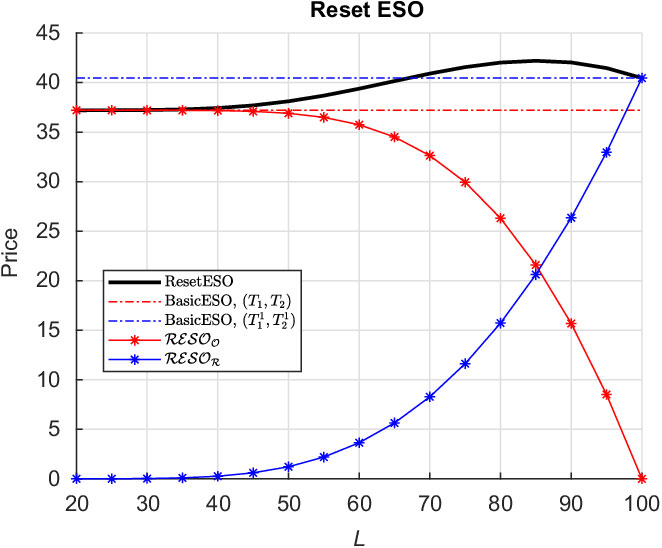
Figure 1 Structure of the Reset Executive Stock Option (ResetESO).

During the vesting period $t \in [0,T_1]$ the Reset ESO consists of two components, an original component and a reset component, with only one being active at any time depending on whether resetting has been triggered. The original component remains active so long as reset is not triggered. In this case, the conditions of the ESO at original granting remain active, which match those of the Basic ESO structure with parameters $(T_1,T_2,K,M)$ . In the event that resetting is triggered, the original ESO component ceases to be active with the reset component becoming immediately active. The reset component will have the structure of a Basic ESO with reset parameters $(T^{\prime}_1,T^{\prime}_2,K',M')$ . We can thus represent the Reset ESO price as the sum of two exotic barrier options. The first is an exotic DO barrier option (representing the original ESO provisions) which is to the knocked-out at first hitting time $\tau_l$ , while the second component is an exotic DI barrier option which is to be knocked-in at $\tau_l$ .

(26) $$\begin{eqnarray}\text{ResetESO} & = \text{D/O} \,\, \underset{ (T_1, T_2, K, M)}{\textrm{BasicESO} } \,\, \text{over} [0,T_1] , \,\text{expiry} \,\, T_2 \end{eqnarray}$$

(27) $$\begin{align} + \text{D/I} \,\, \underset{ (T^{\prime}_1,T^{\prime}_2,K',M')}{\textrm{BasicESO} } \,\, \text{over} [0,T_1] , \, \text{expiry} \,\, T_{2}{\kern-2pt'}\end{align}$$

Using these observations, and armed with the machinery that we have built up in section 2, we may now state the first main result of this paper.

Theorem 3.1 (ResetESO Price). Let $\mathcal{RESO}_\mathcal{O}$ and $\mathcal{RESO}_\mathcal{R}$ represent the original ESO and reset components, respectively, for the Reset ESO structure described in Figure 1 . For all times $t \in [0,T_1]$ , the price of the ResetESO is given by

(28) $$\begin{eqnarray}\textrm{ResetESO} &=& {\mathcal{RESO}_{\mathcal{O}}} + {\mathcal{RESO}_{\mathcal{R}}}\end{eqnarray}$$

Furthermore, the $ t \leq T_1$ prices for the original and reset components are given in terms of a portfolio of three European options $(P^{1}_L,P^{2}_L,P^{3}_L)$ and their mathematical images with respect to the reset level $x=L$ .

(29) $$\begin{eqnarray} {\mathcal{RESO}_{\mathcal{O}}} &=& P^{1}_L - \mathcal{I}_{L} \left\{ P^{1}_L \right\} \end{eqnarray}$$

(30) $$\begin{eqnarray} && \nonumber \\{\mathcal{RESO}_{\mathcal{R}}} &=& P^{2}_L + \mathcal{I}_{L} \left\{ P^{3}_L \right\}\end{eqnarray}$$

The European options $(P^{1}_L,P^{2}_L,P^{3}_L)$ are defined by their $T=T_1$ European pay-offs:

$$\begin{eqnarray*}P^{1}_L|_{T_1} &=& \underset{ (T_1, T_2, K, M)}{{BasicESO} } ( x,0, T_{21} ) \mathbb{1}({x}\! > \! {L}) \\ &&\\P^{2}_L|_{T_1} &=& \underset{ (T^{\prime}_1,T^{\prime}_2,K',M')}{{BasicESO} } ( x, T^{\prime}_{11} ,T^{\prime}_{21} ) \mathbb{1}({x}\! > \! {L}) \\ && \nonumber \\P^{3}_L|_{T_1} &=& \underset{ (T^{\prime}_1,T^{\prime}_2,K',\,M')}{{BasicESO} } ( x, T^{\prime}_{11} ,T^{\prime}_{21} ) \mathbb{1}({x}\! > \! {L})\end{eqnarray*}$$

where $T_{21} = T_2-T_1$ , $T^{\prime}_{11}=T^{\prime}_1-T_1$ , $T^{\prime}_{21}=T^{\prime}_2-T_1$ .

Proof.By the above discussion, the original ESO component may be thought of as an exotic barrier option over $t \in [0,T_1]$ with pay-off at time $T_1$ being given by the $T_1$ value of a BasicESO with structural parameters given by $(T_1, T_2, K, M)$ . We therefore consider the $T_1$ expiry of European option $ P^{1}_L|_{T_1} = \underset{ (T_1, T_2, K, M)}{\textrm{BasicESO} } ( x,0, T_{21} ) \mathbb{1}({x}\! > \! {L})$ . Application of expression (8) from the Method of Images immediately gives rise to expression (29), where $\mathcal{I}_{L}$ represents the Image function with respect to the reset level $x=L$ .

Similarly the DI component may be thought of as an exotic barrier option over $t \in [0,T_1]$ with pay-off at time $T_1$ being given by the $T_1$ value of a BasicESO with structural parameters given by $(T^{\prime}_1,T^{\prime}_2,K',M')$ .

Now consider the general representation for the solution to a DI barrier option for an arbitrary pay-off of the stock price f(x), given by expression (9). For expiry $t=T$ pay-offs, elementary operations give

$$\begin{eqnarray*}V_{\text{DI} }|_T &=& f(x) - \left( f(x) \mathbb{1}({x}\! > \! {B}) - \mathcal{I}_{B} \left\{ f(x) \mathbb{1}({x}\! > \! {B}) \right\} \right) \\[5pt] &=& f(x) \mathbb{1}({x}\! > \! {B}) + \mathcal{I}_{B} \big[ f(x) \mathbb{1}({x}\! > \! {B}) \big] )\end{eqnarray*}$$

By identifying $f(x) = \underset{(T^{\prime}_1,T^{\prime}_2,K',M')}{ \textrm{BasicESO} } ( x, T^{\prime}_{11} ,T^{\prime}_{21} )$ at expiry time $T_1$ , and the lower knock-in barrier level given by the reset level $x=L$ , expression (30) immediately arises.

Remark 3.2. Several points should be noted.

1. • The general representations for the two components of the Reset ESO price given by (29) and (30), respectively, hold for all times $t \leq T_1$ .

2. • The original ESO (DO) component remains active only while the stock price remains above the reset level $x=L$ , and expires worthless once the reset level is breached during the vesting period $t \in [0,T_1]$ .

3. • The reset (DI) component only becomes active once the reset level is breached from above during $t \in [0,T_1]$ , and otherwise expires worthless.

4. • The representation in (28) naturally separates the components of the Reset ESO price into the original stock option component and the reset component as per the IFRS9 financial accounting standard requirements.

3.3 Analytical representation of the no-attrition Reset ESO

Corollary 3.3 Using Theorems 2.2-2.4 , the prices of the two components of the ResetESO may be represented as portfolios comprised solely of power binaries of first and higher orders.

The expression for the original ESO component is given by

(31) $$\begin{eqnarray}&&{\mathcal{RESO}_{\mathcal{O}}}_{T_{1}, T_2 }^{K, M}(x,t) = \nonumber \\ && \quad\quad P^{\scriptscriptstyle +;1}_{\scriptscriptstyle B} - L^{2+{\alpha}}P^{\scriptscriptstyle -;-(1+{\alpha})}_{\scriptscriptstyle {\mbox{{$\frac{L^2}{B}$}\normalsize}}} - K P^{\scriptscriptstyle +;0}_{\scriptscriptstyle B} + K L^{\alpha} P^{\scriptscriptstyle -;-{\alpha}}_{\scriptscriptstyle {\mbox{{$\frac{L^2}{B}$}}}} \nonumber \\ && \quad\quad +{}\, P^{\scriptscriptstyle ++;1}_{\scriptscriptstyle LK} - L^{2+{\alpha}}P^{\scriptscriptstyle --;-(1+{\alpha})}_{\scriptscriptstyle L{\mbox{{$\frac{L^2}{K}$}}}} - B^{2+{\alpha}} P^{\scriptscriptstyle +-;-(1+{\alpha})}_{\scriptscriptstyle L{\mbox{{$\frac{B^2}{K}$}}}} + \left({\mbox{{$\frac{B}{L}$}}}\right)^{2+{\alpha}} P^{\scriptscriptstyle -+;1}_{\scriptscriptstyle L{\mbox{{$\frac{L^2}{B^2}$}}}\!K} \nonumber \\ && \quad\quad -{}\, P^{\scriptscriptstyle ++;1}_{\scriptscriptstyle BK} + L^{2+{\alpha}}P^{\scriptscriptstyle --;-(1+{\alpha})}_{\scriptscriptstyle {\mbox{{$\frac{L^2}{B}$}}}{\mbox{{$\frac{L^2}{K}$}}}} + B^{2+{\alpha}} P^{\scriptscriptstyle +-;-(1+{\alpha})}_{\scriptscriptstyle B{\mbox{{$\frac{B^2}{K}$}}}} - \left( {\mbox{{$\frac{B}{L}$}}}\right)^{2+\alpha} P^{\scriptscriptstyle -+;1}_{\scriptscriptstyle {\mbox{{$\frac{L^2}{B}$}}}\frac{L^2}{B^2}K} \nonumber \\ && \quad\quad -{}\, P^{\scriptscriptstyle ++;1}_{\scriptscriptstyle LB} + L^{2+{\alpha}}P^{\scriptscriptstyle --;-(1+{\alpha})}_{\scriptscriptstyle L{\mbox{{$\frac{L^2}{B}$}}}} + B^{2+{\alpha}} P^{\scriptscriptstyle +-;-(1+{\alpha})}_{\scriptscriptstyle LB} - \left({\mbox{{$\frac{B}{L}$}}}\right)^{2+\alpha} P^{\scriptscriptstyle -+;1}_{\scriptscriptstyle L{\mbox{{$\frac{L^2}{B}$}}}} \nonumber \\ && \quad\quad +{}\, P^{\scriptscriptstyle ++;1}_{\scriptscriptstyle BB} - L^{2+{\alpha}}P^{\scriptscriptstyle --;-(1+{\alpha})}_{\scriptscriptstyle {\mbox{{$\frac{L^2}{B}$}}}{\mbox{{$\frac{L^2}{B}$}}}} - B^{2+{\alpha}} P^{\scriptscriptstyle +-;-(1+{\alpha})}_{\scriptscriptstyle BB} + \left({\mbox{{$\frac{B}{L}$}}}\right)^{2+\alpha} P^{\scriptscriptstyle -+;1}_{\scriptscriptstyle {\mbox{{$\frac{L^2}{B}$}}}{\mbox{{$\frac{L^2}{B}$}}}} \nonumber\\&& \quad\quad -{}\, K P^{\scriptscriptstyle ++;0}_{\scriptscriptstyle LK} + KL^{\alpha} P^{\scriptscriptstyle --;-{\alpha}}_{\scriptscriptstyle L{\mbox{{$\frac{L^2}{K}$}}}} + K B^{{\alpha}} P^{\scriptscriptstyle +-;-{\alpha}}_{\scriptscriptstyle L\frac{B^2}{K}} - K \left({\mbox{{$\frac{B}{L}$}}}\right)^{{\alpha}} P^{\scriptscriptstyle -+;0}_{\scriptscriptstyle L{\mbox{{$\frac{L^2}{B^2}$}}}K} \nonumber \\ &&\quad\quad +{}\, K P^{\scriptscriptstyle ++;0}_{\scriptscriptstyle BK} - K L^{\alpha} P^{\scriptscriptstyle --;-{\alpha}}_{\scriptscriptstyle {\mbox{{$\frac{L^2}{B}$}}}{\mbox{{$\frac{L^2}{K}$}}}} - K B^{{\alpha}} P^{\scriptscriptstyle +-;-{\alpha}}_{\scriptscriptstyle B\frac{B^2}{K}} + K \left( {\mbox{{$\frac{B}{L}$}}}\right)^{{\alpha}} P^{\scriptscriptstyle -+;0}_{\scriptscriptstyle {\mbox{{$\frac{L^2}{B}$}}}{\mbox{{$\frac{L^2}{B^2}$}}}K} \nonumber \\ && \quad\quad +{}\, K P^{\scriptscriptstyle ++;0}_{\scriptscriptstyle LB} - K L^{\alpha} P^{\scriptscriptstyle --;-{\alpha}}_{\scriptscriptstyle L{\mbox{{$\frac{L^2}{B}$}}}} - K B^{{\alpha}} P^{\scriptscriptstyle +-;-{\alpha}}_{\scriptscriptstyle LB} + \left({\mbox{{$\frac{B}{L}$}}}\right)^{\alpha} P^{\scriptscriptstyle -+;0}_{\scriptscriptstyle L{\mbox{{$\frac{L^2}{B}$}}}} \nonumber \\ && \quad -{}\, K P^{\scriptscriptstyle ++;0}_{\scriptscriptstyle BB} + K L^{\alpha} P^{\scriptscriptstyle --;-{\alpha}}_{\scriptscriptstyle {\mbox{{$\frac{L^2}{B}$}}}{\mbox{{$\frac{L^2}{B}$}}}} + K B^{{\alpha}} P^{\scriptscriptstyle +-;-{\alpha}}_{\scriptscriptstyle BB} - K \left( {\mbox{{$\frac{B}{L}$}}}\right)^{{\alpha}} P^{\scriptscriptstyle -+;0}_{\scriptscriptstyle {\mbox{{$\frac{L^2}{B}$}}}{\mbox{{$\frac{L^2}{B}$}}}} \nonumber \\ && \quad +{}\, R \left[ B^{-{\beta}_1} P^{\scriptscriptstyle ++;{\beta}_1}_{\scriptscriptstyle LB} - B^{-{\beta}_1} L^{2{\beta}_1+{\alpha}}P^{\scriptscriptstyle --;{\beta}_2}_{\scriptscriptstyle L{\mbox{{$\frac{L^2}{B}$}}}} + \, B^{-{\beta}_2} P^{\scriptscriptstyle ++;{\beta}_2}_{\scriptscriptstyle LB} - B^{{\beta}_2} L^{2{\beta}_2+{\alpha}} P^{\scriptscriptstyle --;{\beta}_1}_{\scriptscriptstyle L{\mbox{{$\frac{L^2}{B}$}}}} \right . \nonumber \\ && \quad \left. - \,B^{-\beta_1} P^{\scriptscriptstyle ++;{\beta}_1}_{\scriptscriptstyle BB} + B^{-{\beta}_1} L^{2{\beta}_1+{\alpha}} P^{\scriptscriptstyle --;{\beta}_2}_{\scriptscriptstyle {\mbox{{$\frac{L^2}{B}$}}}{\mbox{{$\frac{L^2}{B}$}}}} - \, B^{\scriptscriptstyle -{\beta}_2} P^{\scriptscriptstyle ++;{\beta}_2}_{\scriptscriptstyle BB} + B^{\scriptscriptstyle -{\beta}_2} L^{2{\beta}_2+{\alpha}} P^{\scriptscriptstyle --;{\beta}_1}_{\scriptscriptstyle{\mbox{{$\frac{L^2}{B}$}}}{\mbox{{$\frac{L^2}{B}$}}}} \right]\end{eqnarray}$$

and the expression for the reset component is

(32) $$\begin{eqnarray}&&{\mathcal{RESO}_{\mathcal{R}}}_{T^{\prime}_{1}, T^{\prime}_2 }^{K', M'}(x,t) = \nonumber \\ && \quad\quad\quad P^{\scriptscriptstyle -+;1}_{\scriptscriptstyle L B'} - K' P^{\scriptscriptstyle -+;0}_{\scriptscriptstyle L B'} + L^{2+{\alpha}} P^{\scriptscriptstyle --;-(1+{\alpha})}_{\scriptscriptstyle L {\mbox{{$\frac{L^2}{B'}$}}}} - K'L^{\alpha} P^{\scriptscriptstyle --;-{\alpha}}_{\scriptscriptstyle L {\mbox{{$\frac{L^2}{B'}$}}}} \nonumber \\ && \quad\quad\quad +{}\, P^{\scriptscriptstyle --+;1}_{\scriptscriptstyle L B'K'} - B'^{2+{\alpha}} P^{\scriptscriptstyle ---;-(1+{\alpha})}_{\scriptscriptstyle L B'{\mbox{{$\frac{{B'}^2}{K'}$}}}} + L^{2+{\alpha}} P^{\scriptscriptstyle -+-;-(1+{\alpha})}_{\scriptscriptstyle L {\mbox{{$\frac{L^2}{B'}$}}}{\mbox{{$\frac{L^2}{K'}$}}}} - \left(\frac{B'}{L}\right)^{2+{\alpha}} P^{\scriptscriptstyle -++;1}_{\scriptscriptstyle L {\mbox{{$\frac{L^2}{B'}$}}}{\mbox{{$\frac{L'^2}{B'^2}$}}}K'} \nonumber \\ && \quad\quad\quad -{}\, P^{\scriptscriptstyle --+;1}_{\scriptscriptstyle L B'B'} + B'^{2+{\alpha}} P^{\scriptscriptstyle ---;-(1+{\alpha})}_{\scriptscriptstyle L B'B'} - L^{2+{\alpha}} P^{\scriptscriptstyle -+-;-(1+{\alpha})}_{\scriptscriptstyle L {\mbox{{$\frac{L^2}{B'}$}}}{\mbox{{$\frac{L^2}{B'}$}}}} + \left(\frac{B'}{L}\right)^{2+{\alpha}} P^{\scriptscriptstyle -++;1}_{\scriptscriptstyle L {\mbox{{$\frac{L^2}{B'}$}}}{\mbox{{$\frac{L^2}{B'}$}}}} \nonumber \\ && \quad\quad\quad -{}\, K' P^{\scriptscriptstyle --+;0}_{\scriptscriptstyle L B'K'} + K' B'^{{\alpha}} P^{\scriptscriptstyle ---;-{\alpha}}_{\scriptscriptstyle L B'{\mbox{{$\frac{{B'}^2}{K'}$}}} } - K'L^{{\alpha}} P^{\scriptscriptstyle -+-;-{\alpha}}_{\scriptscriptstyle L {\mbox{{$\frac{L^2}{B'}$}}}{\mbox{{$\frac{L^2}{K'}$}}}} + K' \left(\frac{B'}{L}\right)^{{\alpha}} P^{\scriptscriptstyle -++;0}_{\scriptscriptstyle L {\mbox{{$\frac{L^2}{B'}$}}}{\mbox{{$\frac{L'^2}{B'^2}$}}}K' } \nonumber \\ && \quad\quad\quad +{}\, K' P^{\scriptscriptstyle --+;0}_{\scriptscriptstyle L B'B'} - K' B'^{{\alpha}} P^{\scriptscriptstyle ---;-{\alpha}}_{\scriptscriptstyle B'B'} + K'L^{{\alpha}} P^{\scriptscriptstyle -+-;-{\alpha}}_{\scriptscriptstyle L {\mbox{{$\frac{L^2}{B'}$}}}{\mbox{{$\frac{L^2}{B'}$}}}} - K' \left(\frac{B'}{L}\right)^{{\alpha}} P^{\scriptscriptstyle -++;0}_{\scriptscriptstyle {\mbox{{$\frac{L^2}{B'}$}}}{\mbox{{$\frac{L^2}{B'}$}}}} \nonumber \\ && +{}\, R'\left[ B'^{\scriptscriptstyle -{\beta}_1} P^{\scriptscriptstyle --+;{\beta}_1}_{\scriptscriptstyle L B'B'} + B'^{\scriptscriptstyle -{\beta}_2} P^{\scriptscriptstyle --+;{\beta}_2}_{\scriptscriptstyle L B'B'} + B'^{\scriptscriptstyle -{\beta}_1} L^{2{\beta}_1+{\alpha}} P^{\scriptscriptstyle -+-;{\beta}_2}_{\scriptscriptstyle L {\mbox{{$\frac{L^2}{B'}$}}}{\mbox{{$\frac{L^2}{B'}$}}}} + B'^{\scriptscriptstyle -{\beta}_2} L^{2{\beta}_2+{\alpha}}P^{\scriptscriptstyle -+-;{\beta}_1}_{\scriptscriptstyle L {\mbox{{$\frac{L^2}{B'}$}}}{\mbox{{$\frac{L^2}{B'}$}}} } \right]\end{eqnarray}$$

Remark 3.4 The derivation of equations (31) and (32) is given in the appendix (Appendix B). Although our expressions appear superficially complicated, we note the following:

1. • The 22 terms each for $P^{1}_L$ and its mathematical image gives rise to a total of 44 terms for the original (DO) ESO component of the Reset ESO price.

2. • The 12 terms each for $P^{2}_L$ and $\mathcal{I}\left\{ P^{3}_L\right\}$ give rise to a total of 24 terms in the reset component.

3. • We require second- and third-order power binaries, expressible in terms of the bivariate and trivariate normal distributions.

4. • Despite the apparent complexity of our representation, our formulae are highly symmetric and are quite simple to code and implement.

5. • As per IFRS9 financial accounting requirements, we have provided explicit expressions for the original and reset components separately.

In section 4, we turn our attention to the correct attrition adjustment of our formulae equations (31) and (32), namely to account for involuntary early exercise as required by the IFRS9/AASB9 financial accounting standards. In section 5, we will also compare the accuracy and appropriateness of common methods of approximating attrition adjustment as allowed in the financial reporting standards, namely adjustment by expected time to expiry, with the correct adjustment as given in section 4.

4 Adjustment for Attrition, Automatic Exercise and Forfeiture

Events over the lifetime of an ESO such as unexpected early ill-health retirement or death trigger an unintentional and unforeseen early termination of employment. These events result in pre-vesting forfeiture or post-vesting automatic exercise of the contract. Such unforeseen eventualities are strictly independent of stock price movements. The numerical adjustment to account for this involuntary early exercise readily lends itself to a survival curve approach similar to the modelling of defined benefit pension schemes.

The precise meaning of the term survival usually depends on the context. For a pension fund with compulsory retirement, surviving up to age n means being a paying member of the fund at age n and retiring by the compulsory retirement age at the latest. In the context of ESO valuation, however, survival refers to the grantee surviving in employment. Multiple decrement tables may be used to track several factors for which population membership can be terminated. Simple life tables however might track only one attrition factor. Life and multiple decrement tables are often used in pension fund valuations in large corporations. Tables for common attrition factors are usually obtained from standard actuarial analysis of relevant demographic data.

To incorporate the effects of survival, we employed the multi-state disability and mortality model of Hariyanto (Reference Hariyanto2014) to estimate exit probabilities and model survival factors which we postulate are relevant in the assessment of the competence of an executive to remain in employment after a life contingent event based on health. This model is similar to Rickayzen & Walsh (Reference Rickayzen and Walsh2002) and Leung (Reference Leung2004, Reference Leung2006), and gives similar probabilities to that of the latter two. This model was originally employed to estimate the probability of admission into aged-care facilities, and uses a definition of disability measured in terms of the level of supervision required to conduct basic daily tasks. More generally, the relevant survival characteristics would depend on the precise nature of the employment. The survival functions may be chosen in practice to reflect the survival requirements from the employer.

The ABS Survey of Disability, Ageing and Carers (ABS, 2004) measures disability at the national level. Disability is defined in terms of restriction in conducting so-called core activities which are similar to basic daily tasks, and which we postulate will also be relevant in assessing the fitness of an executive to remain in employment. The ABS measures four levels of restriction: mild, moderate, severe and profound. We employ the discrete multi-state mortality model of Hariyanto (Reference Hariyanto2014) to obtain the estimates of the probabilities of disablement from publicly available cross-sectional data, where we argue analogously that “disability” will represent limitations of senior executives in carrying out their core activities and subsequent loss of employment. We consider five categories which we label as profound disability, severe disability, moderate disability, some disability and no disability, respectively (i.e. no restriction), for the requirements of executives remaining “fit” for employment under the terms of their employment contract. We do this to more accurately model the dynamics of the disability process and to thus obtain a more accurate estimation of the probability of unexpected early or ill-health retirement. For a description of the estimation procedure, see Chapters 3 and 4 of Hariyanto (Reference Hariyanto2014). After estimation of the transition probabilities, survival curves were produced for each of the five states.

Sample data for our analysis were obtained from the HMD, which provides comprehensive mortality and population data for researchers. We obtained cross-sectional mortality rates, death counts and exposure to risk data for Australia from 1921 to 2004. The data are sourced from the ABS, the Australian Centre for Population Research (ACPR) and the Australian Institute of Health and Welfare (AIHW) (Wilmoth et al., Reference Wilmoth, Andreev, Jdanov and Glei2007).

The five survival functions obtained from the respective mortality rates are labelled ABS:0 to ABS:4, as summarised in Table 2. The data are representative of empirically determined criteria for employee survival in employment and are presented in order of increasing stringency. The survival data therefore correspond to an executive being alive with profound disability, severe disability, moderate disability, some disability and no disability, respectively. In the context of employee survival in employment, ABS:0 therefore represents survival data where it is acceptable for an employee to be alive at age n and experience up to profound disability without triggering automatic forfeiture during the vesting period or alternatively triggering automatic early exercise of the ESO during the exercise window. ABS:1 represents survival data where it is acceptable for an employee to be alive at age n and experience up to severe disability without triggering automatic forfeiture during the vesting period or automatic involuntary early exercise during the exercise window. ABS:2 and ABS:3 similarly correspond to moderate disability and some disability, respectively. ABS:4, the most stringent, represents survival data where it is required that the employee be alive at age n and develop no disability whatsoever to avoid triggering automatic forfeiture before vesting or involuntary early exercise after vesting, respectively.

Table 2. ABS survival data used for attrition.

Our analysis remains valid assuming any multiple decrement table for (multiple) causes of pre-vesting forfeiture and post-vesting automatic exercise due to death, ill-health retirement and severe accidents. For any survival-curve data $l_{n}$ , it is a standard exercise to derive the age-specific survival rates $p_{n}$ , representing the probability of surviving one more year at age n. Adopting the convention $p_{n}=0$ for $n \geq N$ , we have

$$\begin{equation*}p_{n} = \frac{l_{n+1}}{l_{n}}\end{equation*}$$

The probability of remaining in the population for further m years at age n are given by the survival functions $_{n}p_{x}$ . The survival functions are readily calculated from the age-specific survival rates:

(33) $$\begin{equation}_{m}p_{n} = \frac{l_{n+m}}{l_{n}} = p_{n} \, p_{n+1} \, \cdot \cdot \cdot \, p_{n+m-1}\end{equation}$$

Given a survival curve $l_{n}$ , the survival functions $_{m}p_{n}$ may be readily obtained as an ensemble for each age n using an elegant linear algebra approach as described in Kyng et al. (Reference Kyng, Konstandatos and Bienek2016).

The survival functions for an ESO grantee of age $\bar{n}$ , namely $_{m}p_{\bar{n}}$ , give the probability that the employee will remain in employment, that is for the contract lasting at least m years. The probability of the employee terminating employment involuntarily and exiting the population due to the attrition factors under consideration in the interval $[\bar{n}+m, \bar{n}+m+1]$ is readily obtained by differencing the survival function: ${}_{m}p_{\bar{n}} - {}_{(m+1)}p_{\bar{n}}$ . Under standard actuarial assumptions, such exit will occur at time $\bar{n}+m+\frac{1}{2}$ that is approximately in the middle of the interval. Given the ensemble of survival functions as defined in equation (33), the correct adjustment to incorporate attrition, that is, pre-vesting forfeiture & post-vesting involuntary exercise, is given by probability-weighted portfolios of our analytical formulae (31) and (32). For an executive of age $\bar{n}$ years at option granting, the final expression for the Reset ESO adjusted for involuntary early exercise is

(34) $$\begin{eqnarray}&& {}_{\text{Adj}}\textrm{ResetESO}_{T_{1}, T_{2}, T^{\prime}_{1} ,T^{\prime}_{2}}^{K, K', M, \bar{n}}(X_{t}, t) = \nonumber \\ && \phantom{+} \quad\quad\quad\quad\quad {}_{(\lfloor T_{2}-t \rfloor)}p_{\bar{n}} \cdot{\mathcal{RESO}_{\mathcal{O}}}_{T_{1}, (t+\lfloor T_{2}-t \rfloor)}^{K, M}(X_{t}, t) \nonumber \\ && \quad\quad\quad\quad\quad\quad + \sum\limits_{m= \lceil T_{1}-t \rceil}^{\lfloor T_{2}-t \rfloor - 1}\Big( {}_{m}p_{\bar{n}} - {}_{(m+1)}p_{\bar{n}} \Big) \cdot{\mathcal{RESO}_{\mathcal{O}}}_{T_{1}, (t+m+\frac{1}{2})}^{K, M}(X_{t}, t) \nonumber \\&& \quad\quad\quad\quad\quad\quad +\, {}_{(\lfloor T^{\prime}_{2}-t \rfloor)}p_{\bar{n}} \cdot{\mathcal{RESO}_{\mathcal{R}}}_{T^{\prime}_{1}, (t+\lfloor T^{\prime}_{2}-t \rfloor)}^{K', M'}(X_{t}, t) \nonumber \\&& \quad\quad\quad\quad\quad\quad + \sum\limits_{m= \lceil T^{\prime}_{1}-t \rceil}^{\lfloor T^{\prime}_{2}-t \rfloor - 1}\Big( {}_{m}p_{\bar{n}} - {}_{(m+1)}p_{\bar{n}} \Big) \cdot{\mathcal{RESO}_{\mathcal{R}}}_{T^{\prime}_{1}, (t+m+\frac{1}{2})}^{K', M'}(X_{t}, t)\end{eqnarray}$$

$\lfloor . \rfloor$ and $\lceil . \rceil$ are the floor and ceiling function, respectively. The first two expressions of equation (34) give the correct probability-weighted attrition adjustment for the original (DO) ESO component whereas the last two lines give the corresponding attrition adjustment for the reset (DI) component.

We finally note that for m and time t such that $(t + m) < T_{1}$ , the Reset ESO will be totally forfeited before vesting and will expire worthless. In the case of $T_{1} \leq (t + m) \leq T_{2}$ , when active, the original component of the ESO will be exercised involuntarily, which corresponds to the original ESO having a reduced time to maturity of $t+m+\frac{1}{2}$ . Similarly for m and time t such that $(t + m) < T^{\prime}_{1}$ after resetting has been triggered, the reset component of the ESO will also be forfeited. When ${T^{\prime}_{1} \leq (t + m) \leq T^{\prime}_{2}}$ , the reset component of the ESO will be exercised involuntarily, with reduced time to maturity $t+m+\frac{1}{2}$ .

5 Numerical Results

In this section, we provide the results of the numerical implementation of our formulae for the original ESO component given by equation (31), the reset component given by equation (32) and the attrition adjustment given by equation (34). We also illustrate the effect of survival considerations on the fair-value valuation, using the Hariyanto (Reference Hariyanto2014) model to specify five different levels of attrition from section 4. We compare our fair-value valuations with the widely used method for mortality adjustment allowed by the IFRS9/AASB9 financial reporting standard; namely adjustment of ESO exercise date with expected time to involuntary early exercise under the considered disability and mortality factors.

The five empirical survival curves obtained in section 4 from the sourced disability and mortality data allowed us to determine five different survival functions which correspond to five specifications for the fitness of an executive to remain in employment as described in Table 2. They correspond to increasing stringency in the definition of “survival” which we argue are relevant for senior executives.

We determined expected times to involuntary early exit for senior executives aged 60, 65 and 70 years at time of option granting under the Hariyanto (Reference Hariyanto2014) model for the five survival curves summarised in Table 2. These expected times to early exit served as a basis for comparison with our survival-adjusted fair-value valuations given by equation (34). Note that two adjusted maturity dates $\left\{ \bar{T}, \bar{T}' \right\}$ are required, one for the original ESO component and the second for the reset component. This is because at all times before vesting, both the original and reset components of the Reset ESO are active from the option-theoretic perspective.

Our implementations were undertaken in Matlab and make use of the normal cumulative distribution function normcdf and the multivariate normal cumulative distribution function mvncdf, both of which are part of the statistics toolbox. Alternatively, algorithms and robust implementations of the bivariate and multivariate cumulative normal distribution functions for numerous programming languages, including Matlab and C++, may be found in Genz (Reference Genz1992) ^{Footnote 7} . Furthermore, when adjusting for attrition using survival functions $_{m}p_{\bar{n}}$ as described in section 4, we employ log-linear interpolation to increase the frequency of interpolation to any desired level.

The following figures were generated for a Reset ESO issued with strike K set at-the-money, with current stock price $x = K = 100$ . We specified a risk-free rate $r = 0.10$ , continuous dividend yield $q = 0.02$ and volatility $\sigma = 0.30$ . Also, upon the event that a resetting is triggered during the vesting period, we specified that the reset component of the ESO to be re-struck to be at-the-money, namely to be re-struck at the stock price at the reset date. Our choice of initial vesting period is given by $T_1 = 2$ and $T_2=5$ , giving a vesting period expiring in 2 years after the initial issuing of the option, to give an initial voluntary early-exercise window $[T_1,T_2]$ of length 3 years. We assume that the employee’s early-exercise behaviour remains the same during the original ESO issuance and after a resetting event by specifying $M = M' = 2.75$ . This choice is justified by the empirical results of Carpenter (Reference Carpenter1998), who found that $M\approx 2.75$ for top executives. With these representative choices for the above parameters, we make two specifications for the voluntary early-exercise window for the reset component.

In all figures except Figure 3, the voluntary early-exercise window for the reset component is given by $[T^{\prime}_1,T^{\prime}_2] = [6,9]$ . Namely, upon reset the vesting period will be extended until time $T^{\prime}_1= 6$ years with new option expiry $T^{\prime}_2 =9$ years. This insures the original voluntary early-exercise window does not overlap with the reset voluntary early-exercise window. Figure 3 was generated with the choice $[T^{\prime}_1,T^{\prime}_2] = [3,6]$ , that is, with overlapping voluntary early-exercise windows for the original and reset components.

Figure 2 Reset ESO price (equation (28)) versus reset level L. Original component $\mathcal{RESO}_{\mathcal{O}}$ (equation (31)), reset component $\mathcal{RESO}_{\mathcal{R}}$ (equation (32)) and non-overlapping exercise windows $[T_1,T_2] = [3,6]$ , $[T^{\prime}_1,T^{\prime}_2] = [6,9]$ .

Figure 3 Reset ESO price (equation (28)) versus reset level L. Original component $\mathcal{RESO}_{\mathcal{O}}$ (equation (31)), reset component $\mathcal{RESO}_{\mathcal{R}}$ (equation (32)) and overlapping exercise windows $[T_1,T_2] = [2,5]$ , $[T^{\prime}_1,T^{\prime}_2] = [3,6]$ .

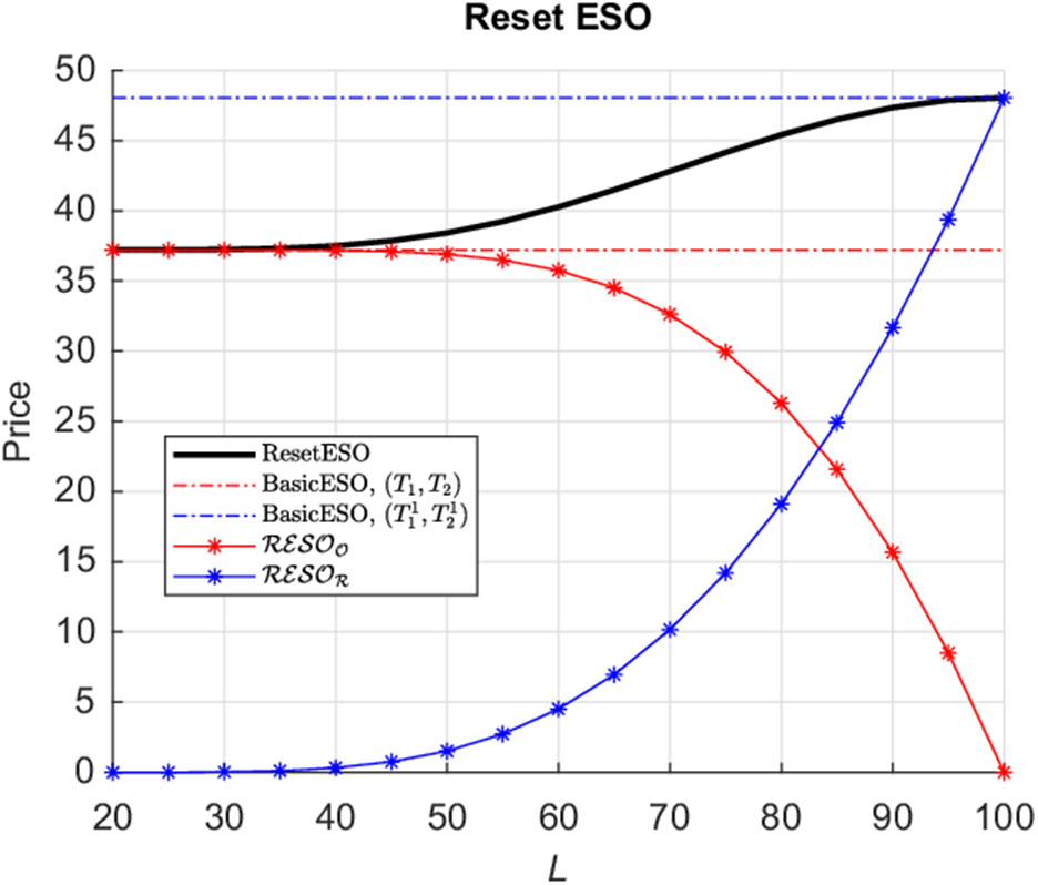
We begin by examining the limiting behaviour of our analytical result. Figure 2 presents numerical results plotted as a function of reset level L. As $L \rightarrow 0$ , we expect that the probability of option resetting will approach zero, so that only the original ESO remains in operation. The reset component will approach zero, and the price given by equation (28) must approach that of the originally issued ESO, namely a BasicESO, given by equation (24) with voluntary early-exercise window coinciding with that of the original ESO component in the Reset ESO structure, $[T_1,T_2] = [2,5]$ . Similarly as L approaches the initial stock price x, the probability of resetting approaches 1, in which case the original ESO is extinguished and the option terms are reset. We therefore expect equation (28) to approach the value of an ESO with the reset features, namely a BasicESO (equation (24)) with voluntary exercise window now given by $[T^{\prime}_1,T^{\prime}_2] = [6,9]$ . This limiting behaviour is reproduced by our formulae in Figure 2. From the time value of options, we expect a BasicESO with the later voluntary exercise window $t \in [6,9]$ is worth more than a BasicESO with earlier voluntary exercise window $t \in [2,5]$ for all values of reset level L. Figure 2 also illustrates the limiting behaviours of the originally issued ESO (equation (31)) and reset component (equation (32)), respectively. As the reset level L rises from 0 to approach the initial stock price at option issuing, namely $L \rightarrow x$ with resetting becoming certain, we expect the reset component (equation (32)) to rise from zero and to approach the value of a BasicESO with voluntary exercise window $[T^{\prime}_1,T^{\prime}_2] = [6,9]$ . Simultaneously we expect the original ESO component (equation (31)) to decrease from that of a BasicESO with voluntary exercise window $[T_1, T_2] = [2,5]$ to zero.

Figure 3 illustrates the effect of overlapping voluntary exercise windows. We observe the same limiting behaviours as in Figure 2, however now the Reset ESO price exceeds that of $\mathcal{RESO}_{\mathcal{R}}$ for some reset levels, reaches a maximum before approaching the value of a BasicESO with the later early-exercise window $[T^{\prime}_1,T^{\prime}_2] = [3,6]$ . With overlapping exercise windows, it therefore becomes possible for an executive to optimally choose a lower reset level $L^*$ to maximise the (survival-unadjusted) fair value of their option. This effect is explainable by the interplay of $\mathcal{RESO}_{\mathcal{O}}$ and $\mathcal{RESO}_{\mathcal{R}}$ , since both have non-zero probabilities of being “alive” at times $t<T_1 \leq T_2$ .

Figure 4 Unadjusted Reset ESO price (equation ((28)) and survival-adjusted price ${}_{\text{Adj}}\textrm{ResetESO}$ (equation (34)) versus reset level L for survival functions in Table 2 for senior executive aged $\bar{n}= 60$ .

Figure 5 Unadjusted Reset ESO price (equation (28)) and survival-adjusted price ${}_{\text{Adj}}\textrm{ResetESO}$ (equation (34)) versus reset level L for survival functions in Table 2 for senior executive aged $\bar{n}= 65$ .

Note that for times $t<T_1$ , both the original ESO component and the reset component will have different expected times to involuntary exercise. For each of the survival functions derived from the data series in Table 2, we determined the (age-dependent) expected times $\left\{ \bar{T}, \bar{T}' \right\}$ to involuntary option exercise, respectively, for the original and reset components of the option, for an executive aged $\bar{n}=60, \, 65$ and 70 years, respectively, at option granting.

Figures 4–6 illustrate the effect of adjustment for survival given by equation (34), as a function of L using the survival functions ${}_{m}p_{\bar{n}}$ described in Table 2.

The topmost curve in Figure 4 indicates the unadjusted price. For an employee age $\bar{n}=60$ years at ESO issuance, we observe that survival-adjustment has an increasingly greater effect on the fair value as the stringency for survival in employment increases from ABS:0 to ABS:4. Increasing stringency consistently lowers the fair value of the Reset ESO for all values of L. Comparing this with Figures 5 and 6, we see that the higher the age of the executive at option granting, the greater the effect of survival adjustment in lowering the overall fair value of their option. This is not surprising, as an employee will have a higher probability of involuntarily exiting employment, the older they are at ESO granting.

Figure 6 Unadjusted Reset ESO price (equation ((28))) and survival-adjusted price ${}_{\text{Adj}}\textrm{ResetESO}$ (equation (34)) versus reset level L for survival functions in Table 2 for senior executive aged $\bar{n}= 70$ .

Another interesting effect arises from the prospect of forfeiture or involuntary early exercise. As observed, the unadjusted fair price varies smoothly from limiting lower and upper levels as outlined above. The introduction of attrition in Figures 4–6 however introduces a peak in the attrition-adjusted ResetESO price. Namely, an optimal reset level $L=L^*$ exists, which maximises the value of the ResetESO for the attrition factors under consideration for each survival curve. This demonstrates an interplay between the time value of the option (which increases with the resetting feature) and the prospect of forfeiture or involuntary exercise due to the survival-adjustment, which negatively affects the option value. That is, survival considerations also introduce the possibility for an employee to optimally specify the stock level triggering option reset to maximise the fair value of their option.

Moreover, as the requirements for survival in employment become more stringent (ABS:0–ABS:4), $L^*$ decreases. With a lower (optimal) reset level, we expect a lower probability of resetting to occur. This has an interesting interpretation that option resetting becomes less important in maximising the fair value of the employee’s option as the survival requirements for remaining in employment become more stringent. Conversely, resetting becomes more important in maximising the fair value of the employee’s option as the survival requirements become less stringent.

Figures 7–9 examine the differences in the evaluation using equation (34) when compared with adjustment using the IFRS9/AASB9 financial reporting standard of expected times to involuntary early exercise $\left\{ \bar{T}, \bar{T}' \right\}$ . The graphs on the left in Figures 7–9 graph the attrition-unadjusted Reset ESO price, the attrition-adjusted price (equation (34)) and the Reset ESO price evaluated with the expected time to involuntary early exercise $\left\{ \bar{T}, \bar{T}' \right\}$ for ABS:4. These are plotted together for comparison as a function of reset level L.

Figure 7 Left: Pricing with expected time to involuntary exercise $\left\{ \bar{T}, \bar{T}' \right\}$ compared with unadjusted (equation (28)) and attrition-adjusted (equation (34)) prices (using ABS:0). Right: Errors in pricing for each survival function in Table 2. Executive aged $\bar{n} = 60$ .

Figure 8 Left: Pricing with expected time to involuntary exercise $\left\{ \bar{T}, \bar{T}' \right\}$ compared with unadjusted (equation (28)) and attrition-adjusted (equation (34)) prices (using ABS:0). Right: Errors in pricing for each survival function in Table 2. Executive aged $\bar{n} = 65$ .

Figure 9 Left: Pricing with expected time to involuntary exercise $\left\{ \bar{T}, \bar{T}' \right\}$ compared with unadjusted (equation (28)) and attrition-adjusted (equation (34)) prices (using ABS:0). Right: Errors in pricing for each survival function in Table 2. Executive aged $\bar{n} = 70$ .

Figure 10 Left: Pricing using $\left\{ \bar{T}, \bar{T}' \right\}$ compared with unadjusted and attrition-adjusted prices (using ABS:0) as a function of exercise multiple M. Right: Errors in pricing for each survival function in Table 2. Executive aged $\bar{n} = 60$ .

We observe an increasing divergence of our fair-value adjusted price equation (34) from the unadjusted price with increasing employee age. We also observe that the prices calculated using the expected times to involuntary exercise $\left\{ \bar{T}, \bar{T}' \right\}$ consistently overestimate the fair-value adjusted price, for all values L. This has an important practical implications for firms using expected times to involuntary exercise to evaluate the book value of these liabilities, as they are potentially recording higher liabilities than strictly necessary.

The plots on the right for each of Figures 7–9 graph the percentage errors arising between equation (34) and evaluation using $\left\{ \bar{T}, \bar{T}' \right\}$ for each of the survival functions from Table 2. For a given executive age at option granting, we observe that the greatest errors occur for the most stringent survival criteria represented by ABS:4, and decrease with decreasing stringency to ABS:0. Also, the errors increase as age increases, for each survival curve in Table 2. We observe a range of errors starting at a relatively insignificant 1–3% for an employee aged 60 with the least stringent survival data (ABS:0) on the right in Figure 7, to a very significant 10– $27.5$ % for an employee aged 70 with the most stringent survival requirements (ABS:4) in Figure 9. The errors arising from evaluation using expected time to involuntary exercise potentially introduce significant overestimates of the liabilities of the firm arising from the granting of the ESO compensation, in particular for the most senior executives.

Figures 10–12 examine the behaviour of our fair-value valuation as the probability of voluntary exercise by the executive diminishes and as the age of option issuance $\bar{n}$ increases. As exercise multiple $M \rightarrow \infty$ from an initial value of around $1.5$ , the probability of early exercise diminishes, as the requirement for voluntary early exercise becomes harder to meet. The graphs on the left of Figures 10–12 show that the unadjusted and adjusted Reset ESO prices reach a maximum value and are bounded above, and then rapidly approach constant levels as M increases. The level is given by the European call option without the early-exercise feature. The maximum value reached approaches the value of the Reset ESO with American call option features in the exercise windows of the original and reset components. Again, the effects of survival on the fair-value valuation become more pronounced as $\bar{n}$ increases. Furthermore, the optimal level $M^*$ also increases (moves to the right) as $\bar{n}$ increases. This gives the interesting interpretation that it becomes less optimal for senior executives to exercise their Reset ESOs early, the older they are at the time their options are issued.

The graphs on the right of Figures 10–12 also demonstrate the errors arising from expected times to involuntary exercise $\left\{ \bar{T}, \bar{T}' \right\}$ . The errors are lowest in Figure 10, where a “profound disability” is consistent with survival in employment, and rise to around 10% if survival in employment requires “no disability.” They increase in Figure 11 and are largest in Figure 12, where the errors range from 5% to almost 19%, respectively.

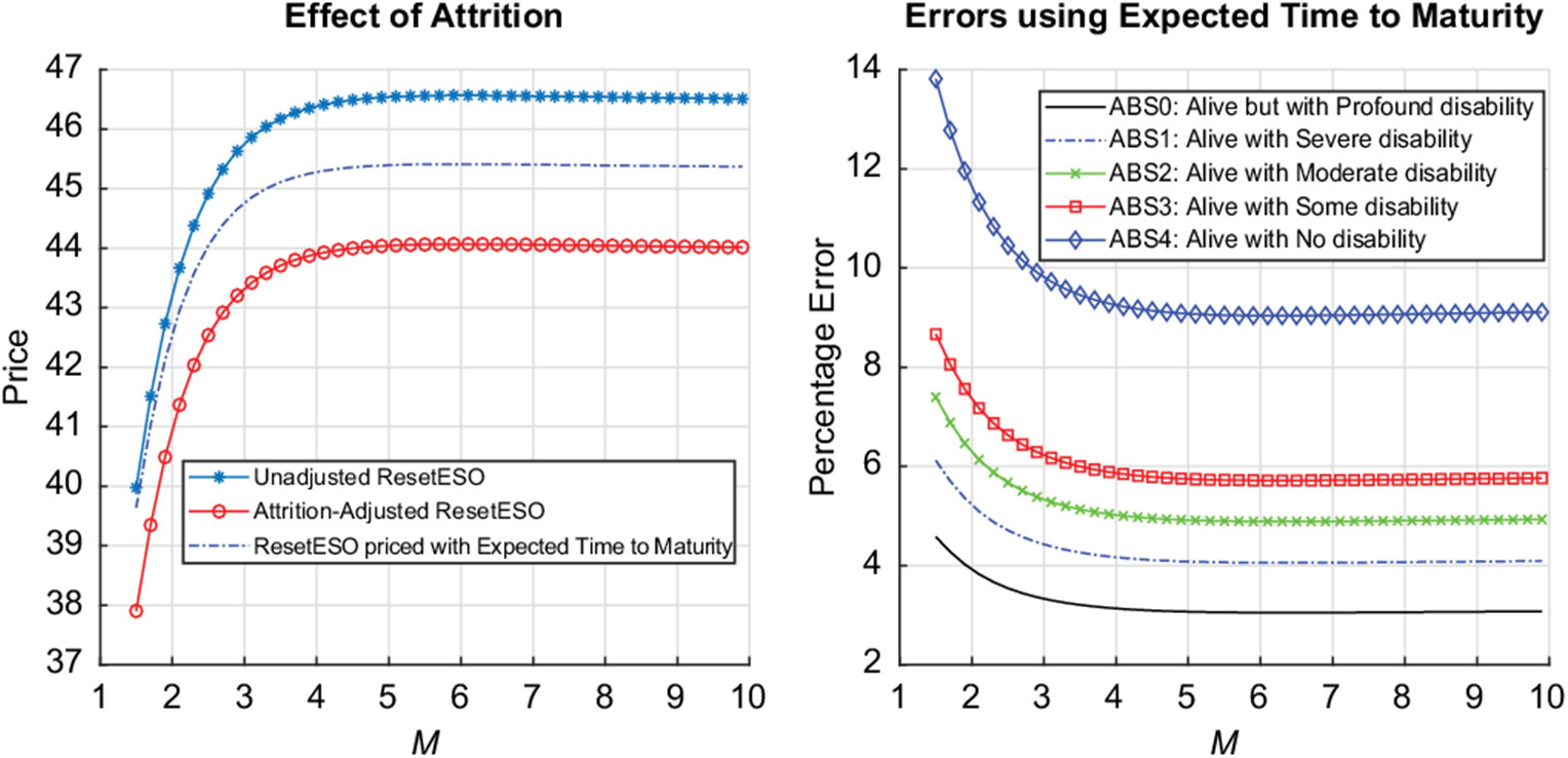
Figure 11 Left: Pricing using $\left\{ \bar{T}, \bar{T}' \right\}$ compared with unadjusted and attrition-adjusted prices (using ABS:0) as a function of exercise multiple M. Right: Errors in pricing for each survival function in Table 2. Executive aged $\bar{n} = 65$ .

Figure 12 Left: Pricing using $\left\{ \bar{T}, \bar{T}' \right\}$ compared with unadjusted and attrition-adjusted prices (using ABS:0) as a function of exercise multiple M. Right: Errors in pricing for each survival function in Table 2. Executive aged $\bar{n} = 70$ .

Again this illustrates that the use of expected time to exercise to evaluate firm liabilities may introduce significant overestimates compared to the fair-value valuation, and that the overestimates increase in a predictable manner with increasing age (and seniority) of the executives.

6 Conclusion

We produced a novel closed-form representation of the fair value for an Executive Stock Option with reset features incorporating the most general resetting of strike price, vesting period, voluntary early-exercise characterisation and maturity date. Using the exercise multiple approach of Hull & White (Reference Hull and White2004) to model the early-exercise behaviour of executives and applying several new lemmas, we developed a model to express the fair-value Reset ESO price as the sum of a component for the originally issued option and a reset component for the reissued option, with prices expressed in terms of novel portfolios of standardised European instruments which we refer to as first-, second- and third-order power binary options. We employed the discrete multi-state model of Hariyanto (Reference Hariyanto2014) to estimate probabilities of disablement, and argued analogously that states of disability we considered represent appropriate survival criteria for senior executives for the purposes of involuntary exit from employment. Using Australian data sourced from the HMD, we estimated five different survival functions corresponding to five different levels of disability consistent with executives remaining fit for employment, and applied the corresponding adjustments to illustrate the effects of survival and mortality triggering involuntary early exercise on the fair value of the Reset ESO price. Comparing our numerical results with the commonly used survival adjustment under the IFRS9/AASB9 financial reporting standard of valuation by expected time to involuntary early option exercise, we demonstrated a systematic and potentially significant overestimate of the liabilities compared to the theoretical fair value as given by our formulae. We observed errors ranging from 3% to as high as 27% for senior executives. We demonstrated that survival adjustment or alternatively overlapping vesting periods in the original ESO and reset component allow for the optimal selection of the stock level triggering option resetting, to maximise option value. Our results arise as theoretical consequences of our valuation formulae and not as empirical observations. Our fair-value valuation is consistent with all the mandated requirements of the currently operational IFRS9 standard and its Australian implementation AASB9, and may be of significant benefit to firms which may be overestimating the financial liabilities arising from ESOs with reset features issued to their senior executives, or alternatively to senior executives wishing to maximise the value of their stock options.