
1. Introduction
Primary cementing is an industrial operation that has attracted the attention of the fluid mechanics community for 2–3 decades (Nelson Reference Nelson1990; Bittleston, Ferguson & Frigaard Reference Bittleston, Ferguson and Frigaard2002). It remains inadequately understood due to both complexity and evolution of the industrial process. In this operation a sequence of fluids is pumped down the inside of a steel casing, to the bottom of an oil or gas well, returning upwards in the annular space between formation wall and exterior of the casing; figure 1(a). The aim of the process is to remove the drilling fluid and other residue from the well, replacing it with a cement slurry.

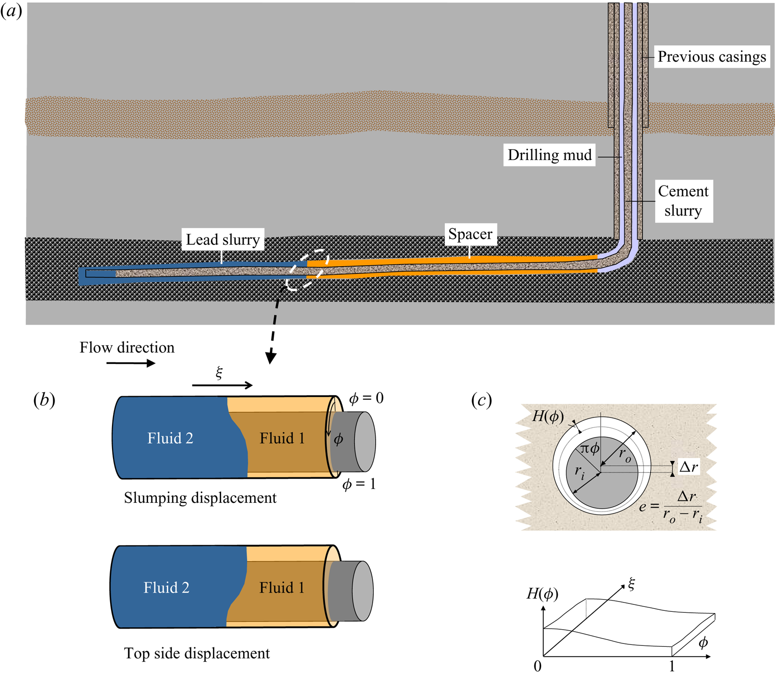
Figure 1. Horizontal primary cementing: (a) typical fluid sequence in a displacement; (b) unit displacement operation in horizontal section illustrating top and slumping modes; (c) model set-up from Carrasco-Teja et al. (Reference Carrasco-Teja, Frigaard, Seymour and Storey2008).
Avoiding excessive contamination and ensuring that the cement slurry bonds well with both the steel casing and formation wall, means that the fully set cement can form an effective hydraulic seal of the annulus as well as give structural support. Hydraulic zonal isolation is needed for two main reasons: leakage compromises well productivity and can have environmental/health consequences, e.g. polluted aquifers, subsurface ecosystems, methane emissions. Leakage within the well is difficult to locate and expensive to fix. Since the late 1990s there has been a worldwide trend towards drilling horizontal wells, meaning that the last part of the well is approximately horizontal, to align with the hydrocarbon-bearing reservoir; figure 1(a). For example, in British Columbia, vertical wells accounted for  $>$75 % of wells drilled prior to 2000 but
  $\approx$95 % of wells drilled in the last decade have been horizontal (Trudel et al. Reference Trudel, Bizhani, Zare and Frigaard2019).
From the fluid mechanics perspective, since the fluids involved in cementing exhibit significant density contrasts, it is not surprising that displacement flows in horizontal wells behave quite differently from those in vertical wells. Trudel et al. (Reference Trudel, Bizhani, Zare and Frigaard2019) found that over  $28\,\%$ of British Columbia wells drilled in 2010–2018 reported leakage, albeit often minor. Although precise causality was not determined, what is clear is that significant numbers of wells are not sealing adequately and from this perspective the cementing operation has failed. There are many difficulties with cementing and indeed many of those specific to deviated and horizontal wells were known long before the upsurge in horizontal drilling (Keller et al. Reference Keller, Crook, Haut and Kulakofaky1987). In this paper we focus only on fluid mechanics issues in horizontal narrow eccentric annular displacement flows.
As illustrated in figure 1(a) the flow consists of a sequence of fluids, each displacing the fluid in front. A typical mean annular gap is 2–3 cm, production casing outer diameters are 114–245 mm (4.5–9.625 in.) and lengths of cemented casing can be  $10^2\text {--}10^3$ m, i.e. the annulus is relatively narrow and very long. The fluid volumes pumped are such that we can consider each displacement problem as consisting of two fluids only. Typically one or more preflushes (spacers or washes) precede the cement slurries. The drilling mud can be oil based or water based with different formulations according to the desired function: drilling, removing cuttings or conditioning the well. Muds are non-Newtonian shear thinning fluids, often with a yield stress. Washes (typically Newtonian with low density and viscosity) are sometimes used to prepare the interval to be cemented. The idea is to leave the walls water wet to ease the bonding of cement and improve displacement of the mud. Spacer fluids are rheologically designed to remove the drilling mud and also provide a buffer between mud and cement, since these may be chemically incompatible. Cement slurries are shear thinning, often thixotropic and with a modest yield stress.
In this preliminary study we only consider Newtonian fluids. First, there does not appear to be a comprehensive experimental study of Newtonian displacement flows in horizontal annuli. Secondly, building our knowledge on simpler fluids will allow us to draw conclusions before introducing non-Newtonian complexities. Thirdly, although there are definitely flow features that arise due to rheology, in particular the yield stress, the theoretical understanding of horizontal cementing that exists focuses primarily on the competition between buoyancy and eccentricity: rheology is often a secondary effect.
In the 1990s a range of studies were performed to validate general understanding of vertical well displacements, as captured in design rules such as Couturier et al. (Reference Couturier, Guillot, Hendriks and Callet1990). Experiments date back to the 1960s (McLean, Manry & Whitaker Reference McLean, Manry and Whitaker1967) and have used both field fluids and rheologically similar laboratory fluids. Extensive studies such as Jakobsen et al. (Reference Jakobsen, Sterri, Saasen, Aas, Kjosnes and Vigen1991), Tehrani, Ferguson & Bittleston (Reference Tehrani, Ferguson and Bittleston1992) and Tehrani, Bittleston & Long (Reference Tehrani, Bittleston and Long1993) were compared favourably with simulation tools of the time. A notable feature of these experiments was that measurement was primarily via conductivity probes, e.g. positioned azimuthally around the annulus close to the exit. This method has the advantage of giving an objective measure of the concentration of the fluids that pass between the probes: generally, a salt is used to increase conductivity of one fluid. Integrated over time these measurements give a direct measure of the displacement efficiency, i.e. how much of the in situ fluid has been displaced. However, displacement efficiency is a crude measure when defects are typically on the narrow side of the eccentric annulus. Maleki & Frigaard (Reference Maleki and Frigaard2019) show that displacement efficiencies as high as 90 % can result from flows with obviously poor displacement.
Conductivity can give more local information, e.g. an azimuthal distribution of displacement efficiency as in Tehrani et al. (Reference Tehrani, Ferguson and Bittleston1992), or by the use of multiple axial banks of probes as in Lund et al. (Reference Lund, Ytrehus, Taghipour, Divyankar and Stavanger2018) and Skadsem et al. (Reference Skadsem, Kragset, Lund, Ytrehus and Taghipour2019). However, typically the number of probes remains limited and spatio-temporal features of the flow remain obscured, e.g. the distribution of fluids across the annular gap. More recent studies have tended to use visualization of the flow, as with Malekmohammadi et al. (Reference Malekmohammadi, Carrasco-Teja, Storey, Frigaard and Martinez2010) and Deawwanich (Reference Deawwanich2013). Visualization has distinct advantages in that one can observe flow structures in the fluid, perform post-processing for quantitative information and observe e.g. residual fluid channels, wall layers and flow instabilities. To be effective, the fluids are coloured/dyed and at least one should be transparent. This can limit the range of fluids available with suitable rheological properties, which is the drawback.
In the vertical part of the well a positive buoyancy gradient aids displacement (Couturier et al. Reference Couturier, Guillot, Hendriks and Callet1990): density differences in the range 0–300 kg m $^{-3}$ are common. Therefore, it is usual that more dense fluids displace less dense fluids in the preceding horizontal sections, but not always, e.g. washes are typically less dense than drilling mud. Eccentricity of the annulus towards the bottom of the well is usual, due to the high density of the steel casing. Eccentricity promotes flow along the wider part of the well whereas density differences promote density stable stratification. Thus, for a unit operation of fluid 2 displacing fluid 1, two characteristic flow types are common: ‘top side’ or slumping (figure 1b). If the interface fully stratifies fluid displacement will be ineffective. The ideal situation involves a steadily propagating displacement front. This framework conceptualizes theoretical understanding of horizontal cementing displacements, insofar as it has developed, and rests on the work of Carrasco-Teja et al. (Reference Carrasco-Teja, Frigaard, Seymour and Storey2008).
This paper presents the results of approximately 300 laboratory experiments, carried out using Newtonian fluids in a dimensionally scaled and purpose-built eccentric annular apparatus. The focus is on understanding the main effects of buoyancy, eccentricity and viscosity ratio, on the effectiveness of displacement, exposing the physical phenomena observable in experiments and analysing flow regimes. The paper advances partly in parallel with predictions from the model developed by Carrasco-Teja et al. (Reference Carrasco-Teja, Frigaard, Seymour and Storey2008), which we outline below in § 2. Section 3 deals with experimental design. This starts with a dimensional analysis, then describes the choice of fluids, features of the experimental apparatus, visualization and test procedures. The results are presented in three sections. In § 4 we look at the main competition between buoyancy and eccentricity in terms of whether the front advances primarily on the top or bottom side (figure 1b), and comparing with model predictions of the same. Section 5 deals with displacement front dynamics. We highlight some of the difficulties in visualizing the displacement flow in such long domains. We compare front velocities with model predictions and finally we characterize the experimental displacements as an advection–diffusion process. Finally, § 6 outlines some of the flow instabilities observed in the experiments. The paper ends with a short discussion. A sequel to our study is directed towards a comparison of the experiments reported in this paper with three-dimensional (3-D) simulations.
2. Modelling primary cementing flows
Carrasco-Teja et al. (Reference Carrasco-Teja, Frigaard, Seymour and Storey2008) use a Hele-Shaw scaling approach, resulting in simplifications that allow for both quick numerical simulation and analysis. Hence questions such as whether the displacement is steady or stratifies can be answered. The underlying Hele-Shaw model is identical with that analysed earlier for vertical annular displacement flows (Bittleston et al. Reference Bittleston, Ferguson and Frigaard2002; Pelipenko & Frigaard Reference Pelipenko and Frigaard2004a,Reference Pelipenko and Frigaardb,Reference Pelipenko and Frigaardc) and to that recently extended towards other flow regimes (Maleki & Frigaard Reference Maleki and Frigaard2017, Reference Maleki and Frigaard2018, Reference Maleki and Frigaard2019). Variants of the underlying model are becoming widespread (Aranha et al. Reference Aranha, Miranda, Cardoso, Campos, Martins, Gomes, de Araujo and Carvalho2012; Tardy & Bittleston Reference Tardy and Bittleston2016) as are apparently similar engineering software, developed in-house by many companies. This style of model has also become regularly used industrially for cementing case studies, job designs and post-job evaluations, e.g. Osayande et al. (Reference Osayande, Isgenderov, Bogaerts, Kurawle and Florez2004), Bogaerts et al. (Reference Bogaerts, Azwar, Bellabarba, Dooply and Salehpour2015), Guo et al. (Reference Guo, Qi, Zheng, Taoutaou, Wang, An and Guo2015) and Tardy et al. (Reference Tardy, Flamant, Lac, Parry, Sri Sutama and Baggini Almagro2017). In general, model results compare favourably with evidence of cement positioning from post-placement logging of wells. However, well cementing is not an operation that is easily accessible to allow direct measurement of the flow or finished cement integrity. This motivates both laboratory-scale experiments and computational simulation.
There have been attempts to extend the Hele-Shaw style of displacement model in various directions. Firstly, movement of the casing is used to improve displacement, e.g. by rotation, and this has been addressed by Carrasco-Teja & Frigaard (Reference Carrasco-Teja and Frigaard2009), Carrasco-Teja & Frigaard (Reference Carrasco-Teja and Frigaard2010), Tardy & Bittleston (Reference Tardy and Bittleston2016) and Tardy (Reference Tardy2018). Three-dimensional simulations of annular displacement flows were first developed in the late 1990s but were too slow for practical usage (Szabo & Hassager Reference Szabo and Hassager1997; Vefring et al. Reference Vefring, Bjorkevoll, Hansen, Sterri, Saevareid, Aas and Merlo1997). In recent years interest has revived in these methods as open source and other computational codes have become widely accessible and multi-processor computations have made such calculations manageable at reasonable resolutions over increasingly long annuli and even for non-Newtonian fluids, e.g. Kragset & Skadsem (Reference Kragset and Skadsem2018), Etrati & Frigaard (Reference Etrati and Frigaard2019) and Skadsem et al. (Reference Skadsem, Kragset, Lund, Ytrehus and Taghipour2019). Those 3-D simulations that have been published certainly expose flow features not present in Hele-Shaw models: inertial effects and flow features on the scale of the annular gap. The main restriction computationally is to have resolution of gap-scale features, e.g. Allouche, Frigaard & Sona (Reference Allouche, Frigaard and Sona2000) and Zare, Roustaei & Frigaard (Reference Zare, Roustaei and Frigaard2017), while studying azimuthal features of secondary flows and the lengthwise development along the annulus, over industrially relevant lengths. In a displacement flow where unsteady features are to be resolved, the time scale of flow also increases proportionate to the length of annulus, making the computational cost severe. Realistically, we are not yet able to simulate a full well using these methods in a scientifically rigorous way, but lengths of the order of tens of metres are feasible.
We now outline the Newtonian version of the mathematical model of Carrasco-Teja et al. (Reference Carrasco-Teja, Frigaard, Seymour and Storey2008), which is identical with that described in Bittleston et al. (Reference Bittleston, Ferguson and Frigaard2002) and recently extended by Maleki & Frigaard (Reference Maleki and Frigaard2017). It is the latter of these that we use for our computations later in the paper. Simplification results from the premise that the annular gap is narrow relative to azimuthal and axial length scales. This reduces the Navier–Stokes equations to a shear flow in the direction of the modified pressure gradient, at leading order. Integration across the gap width and cross-differentiation eliminates the pressure, resulting in a 2-D elliptic problem for the gap-averaged streamfunction  $\varPsi$. The streamfunction equation is coupled to a transport equation for the gap-averaged fluid concentrations
 \begin{equation} \frac{\partial }{\partial t} [ H\bar{c} ] +\frac{\partial }{ \partial \phi } [ H\bar{v}\ \bar{c} ] +\frac{\partial }{ \partial \xi } [ H\bar{w}\ \bar{c} ] =0. \end{equation}
Here,  $\bar {c} \in [0,1]$ is the concentration of displacing fluid 2,
  $\phi \in [0,1]$ denotes the azimuthal coordinate and
  $\xi$ the axial coordinate, measured from the start of the annulus. The annular half-gap width
  $H$ is defined by
 \begin{equation} H(\phi )=1+e\cos \pi \phi , \end{equation}
which is a narrow-gap approximation:  $e\in [0,1]$ is the eccentricity; see figure 1(c). The annulus is initially full of fluid 1, which is displaced by fluid 2. Due to the large Péclet number molecular diffusion has been ignored. We note that the gap-averaged approximation of the advective transport effectively neglects dispersion on the scale of the gap, which is a deficiency exposed in this paper. Boundary conditions for (2.1) are the symmetry of concentration at
  $\phi =0, 1$, and specification of inflow fluid concentration at
  $\xi =0, Z$, i.e.
  $\bar {c} = 1$. Averaged velocity components in the
  $(\phi ,\xi )$-directions are
  $(\bar {v},\bar {w})$ which are defined in terms of a streamfunction
  $\varPsi$
 \begin{equation} \frac{\partial \varPsi }{\partial \phi }=H\bar{w}, \quad \frac{ \partial \varPsi }{\partial \xi }=-H\bar{v}. \end{equation}
For Newtonian fluids the elliptic equation for the streamfunction is
 \begin{equation} \boldsymbol{\nabla} \boldsymbol{\cdot} \left[ \frac{3\mu (\bar{c})}{H^3} \boldsymbol{\nabla} \varPsi + \left( 0,\frac{\rho (\bar{c}) \sin \pi \phi }{St}\right) \right]=0, \end{equation}
where  $St$ is a Stokes number, defined later; see Bittleston et al. (Reference Bittleston, Ferguson and Frigaard2002) for Herschel–Bulkley fluids. The dimensionless viscosity
  $\mu (\bar {c})$ and density
  $\rho (\bar {c})$ depend on the fluids present in the annulus, i.e.
  $\bar {c}$. Boundary conditions are
 \begin{gather} \varPsi (0,\xi ,t)=0, \quad \varPsi (1,\xi ,t)=1, \end{gather}
 \begin{gather}\frac{\partial \varPsi }{\partial \xi}(\phi ,Z,t)=0,\quad \frac{\partial \varPsi }{\partial \xi }(\phi ,0,t)=0. \end{gather}
To recover dimensional quantities, the axial and azimuthal velocities have been scaled with the mean imposed flow velocity,  $\hat {w}_0$, lengths with the half-circumference,
  $\pi (\hat {r}_{o}+\hat {r}_{i})/2$, viscosity and density are scaled with the displaced fluid 1 properties. A shear stress scale is defined as
  $\hat {\mu }_1\hat {w}_0/\hat {d}$, where
  $\hat {d}=(\hat {r} _{o}-\hat {r}_{i})/2$. The pressure gradient balances with the leading-order shear-stress scale, as usual in a Hele-Shaw flow, defining the pressure scale.
In Carrasco-Teja et al. (Reference Carrasco-Teja, Frigaard, Seymour and Storey2008), as well as solving the above two-dimensional gap-averaged (2DGA) model for a range of flows, the authors consider explicitly the competition between density differences (buoyancy) and annular eccentricity that results in the top side and slumping displacements illustrated in figure 1(b). In the top side displacement the effects of eccentricity ( $e>0$) are dominant and the displacement front advances along the wider top of the annulus. If fluid 2 is denser this stratification eventually results in a density unstable situation. In the slumping displacement the front slumps to the bottom of the annulus and elongates. Carrasco-Teja et al. (Reference Carrasco-Teja, Frigaard, Seymour and Storey2008) use a thin-film/lubrication style model (applied to the Hele-Shaw model above), to show that the interface may elongate to an extent where buoyancy effects reduce and a steadily propagating front results. For other parameters, the slump continues to stretch out: an unsteady displacement. Analysis of the thin-film/lubrication model allows for parametric predictions to be made of the transition between steady and unsteady displacement regimes.
3. Experimental design
Before describing our experimental set-up, we give an overview of the field setting that we are attempting to simulate and discuss dimensional analysis of a typical displacement. Annular displacement proceeds from the bottom of the well upwards to surface. Thus, any horizontal section of a well is typically at the start of the displacement. The steel casing/liner to be cemented in place is the production casing and would commonly have outer diameter in the range 114–245 mm (4.5–9.625 in.). Larger diameters occur for the previous casings, found higher up in the well; see figure 1(a). The borehole diameter typically leaves a mean annular gap of 20–30 mm, so that an aspect ratio of radial and circumferential length scales,  $\delta = (\hat {r}_0-\hat {r}_i)/(\hat {r}_0+\hat {r}_i)\pi \in [0.03,0.1]$ is to be expected. The borehole may be relatively smooth or uneven, due to geological variations and drilling practices. The well trajectory varies along the annulus, eventually becoming vertical and cemented sections are
  $\sim 10^2\text {--}10^3$ m in length.
Here we consider only a long straight horizontal section of annulus. Dimensional analysis of the displacement flow of two Newtonian fluids along a uniform horizontal eccentric annulus shows that there are seven different non-dimensional parameters involved: the aspect ratio  $\delta$; the Reynolds number,
  $Re = \hat {\rho }_1\hat {w}_0 \hat {d}/\hat {\mu }_1$; the Péclet number
  $Pe = \hat {w}_0\hat {d}/\hat {D}$; the Stokes number,
  $St = \hat {\mu }_1\hat {w}_0/(\hat {\rho }_1\hat {g}(\hat {d})^2)$; the density ratio,
  $\rho = \hat {\rho }_2/\hat {\rho }_1$; the viscosity ratio,
  $\hat {\mu }_2/\hat {\mu }_1$; and the eccentricity,
  $e = {\rm \Delta} \hat {r} / (\hat {r}_o-\hat {r}_i)$. Note that
  ${\rm \Delta} \hat {r}$ (hence
  $e$) might also be negative; see figure 1(c). Possibly also relevant is the scaled length, which determines the time scale of the displacement. Simplification comes from the high Péclet number, meaning that molecular diffusion is not relevant.
The narrow-gap approach of Carrasco-Teja et al. (Reference Carrasco-Teja, Frigaard, Seymour and Storey2008) combines the density ratio and Stokes number to give a buoyancy number:  $b = (\hat {\rho }_2 - \hat {\rho }_1)\hat {g}\hat {d}^2/(\hat {\mu }_1\hat {w}_0)$, and neglects inertial effects under the assumption that
  $\delta Re \ll 1$. This leaves only
  $(b,e,\hat {\mu }_2/\hat {\mu }_1)$. The buoyancy number balances buoyant and viscous stresses over the scale of the annular gap:
  $b>0$, corresponds to a heavier fluid displacing a lighter one and vice versa. Since buoyancy is one of the main flow-controlling parameters in these flows, we study a wide range
  $b = -10^3 \ {\rm to} \ 10^3$, typical of field conditions. Although we compare against the predictions of Carrasco-Teja et al. (Reference Carrasco-Teja, Frigaard, Seymour and Storey2008), in practice
  $\delta Re \ll 1$ is not always found. Although laminar regimes are preferred in cementing horizontal wells,
  $Re \sim 1\text {--}1000$ are common. We consider a similar range for our experiments.
Regarding rheology, here we use pairs of Newtonian fluids. Direct flow visualization is the main method used for analysis and therefore use transparent fluids. In most of our experiments one fluid is water. To achieve different densities we have used aqueous solutions of NaCl and CaCl $_2$ at different concentrations. More viscous fluids were prepared with different proportions of glycerol and water. Isodense displacements with enhanced viscosity difference were achieved by increasing the density of the less viscous fluid using salt. Table 1 shows examples of displacing and displaced fluids used. The viscosity ratios achieved are in the range of 0.09–12, which modestly covers field values. Depending on the density and viscosity ratios, these pairings might be considered to represent any of: mud/wash, mud/spacer, wash/spacer, spacer/cement combinations, as there is no universal practice for fluid property selection.
Table 1. Typical fluids pairs and formulations.

To summarize, discounting non-Newtonian effects for now, we can achieve dimensional similarity with respect to field conditions for laminar displacement flows, under the above considerations. Although the main dimensionless parameters are  $e, b, \hat {\mu }_2/\hat {\mu }_1$, as we move away from narrow-gap approximation regimes inertia may become important
  $\delta Re \not \ll 1$. We have conducted
  $\approx$300 experiments to explore these parameters, with approximately 20 % of these repeated to validate the apparatus and measurement techniques. A summary of the parametric space explored is given in table 2.
Table 2. Dimensionless parameter ranges of our experimental study.

3.1. Annular apparatus
Figure 2 shows a simplified version of the flow loop used. The central component of the set-up is a 4.8 m long transparent annulus. The length is achieved by joining four 1.2 m sections, with annulus formed by an inner aluminium pipe (outer diameter 34.925 mm) and an outer Plexiglass pipe (inner diameter 44.45 mm). The aluminium pipe was specially machined to a 0.127 mm outer diameter tolerance and is connected using an internal pipe joint. The outer transparent pipes are joined together within a collar held by the friction of an o-ring seal, with small gap between pipes to allow thermal expansion and avoid cracking. The general dimensions of our apparatus are listed in table 3. While not a very narrow gap, we note that  $\delta$ is in the lower part of the range typical of horizontal wells. The annulus length was made to be sufficient for laminar flows to develop, based on either annular gap or circumferential length scales.

Figure 2. Experimental set-up schematic.
Table 3. Apparatus dimensions.

A positive displacement pump delivers the displacing fluid at a constant flow rate for the experiment. An additional centrifugal pump is used to fill the annulus with the displaced fluid and for cleaning between experiments. Both pumps are controlled by a variable frequency driver (VFD). In the displacing fluid line we have installed a manually operated globe valve and bypass, in order to vary the flow rate below the VFD rate. Downstream of the gate valve, a flow straightener is attached to the inner aluminium pipe to mitigate entry and development effects. An electromagnetic flow meter records the imposed flow rate. The flow meter accuracy, pumps and globe valve were calibrated by measuring the mass of fluid pumped over a fixed time interval.
3.1.1. Eccentricity adjustment
We are able to set the eccentricity of the inner pipe, anywhere from resting at the bottom of the Plexiglas pipe ( $e= 1$), to reaching the top (
 $e=-1$). The eccentricity of each section is set using 5 in-house made eccentricity devices. The design of the device is based on a 1.587 mm diameter wire that cross the collar and it is fastened to the inner pipe (figure 3a). In one end, the wire crosses a stud (threaded) and then it is clamped to an adjustment knob. On the other end, the wire is fixed to a spring-indicator assembly. To raise/lower the inner aluminium pipe (see figure 3b), the adjustment knob is turned and distance measured on a dial. This allows us to set the eccentric displacement within a tolerance of 0.254 mm.

Figure 3. (a) Transverse cut of eccentricity adjustment device. (b) Fully eccentric position. (c) Cross-sectional view of the mirror arrangement.
One practical difficulty of scaling down is that the annular gap becomes very small, so that deflection of the inner body must be minimized. The eccentricity devices provide support to the inner aluminium pipe at the ends of each section. We estimate the bending using an elastic beam equation (uniform load with fixed ends). This gives an estimate of maximum deflection:  $(\hat {W} \hat {l}^4)/(384\hat {E}\hat {I}) \approx 0.01$ mm, where
  $\hat {W}$ is the unit weight of the pipe (N m
 $^{-1}$),
  $\hat {E}$ is Young's modulus (N m
 $^{-2}$) and
  $\hat {I}$ is the second moment of area (m
 $^4$). This deflection is an order of magnitude below both the tolerance of the eccentricity measurement and the acrylic pipe OD tolerance. Moreover, during the experiment the annulus is filled with fluid, which reduces the effective
  $\hat {W}$ via buoyancy.
3.1.2. Flow visualization
Each section of the annulus is contained inside a transparent rectangular Plexiglas box, (a fish tank), filled with glycerol. The purpose of the tank is to minimize optical aberrations due to different air–Plexiglas diffraction indices, and due to curvature of the pipe. The annulus visualization is enhanced by a mirror arrangement, illustrated in figure 3(c). Two first-surface mirrors are placed at 45 $^\circ$ angles from the two back vertices of the fish tank. In this way, the bottom, back and top views of the annulus are reflected to the camera.
Our main quantitative measurement is visual. The small aspect ratio of the set-up limits the field of view that a single camera can provide at a reasonable resolution across the annular gap. To overcome this, the experiment is recorded with four cameras in series. The first and last cameras, Cam 2 and Cam 3 are positioned to give a resolution of approximately 2 pixel mm $^{-1}$. Cam 0 and Cam 1 have approximate resolution 1 pixel mm
 $^{-1}$ at the laboratory working distance. Slightly different frame rates (1–4 f.p.s.) are used to avoid data collapse issues on the network during download.
3.2. Test procedure
The fluids are prepared/mixed and held in two tanks. A sample of each fluid was taken before starting each experiment. Densities were measured using an electrical densiometer. Viscosities were measured using a Malvern Kinexus rheometer at the in-site recorded temperature of the fluid. The displacing fluid is marked using non-waterproof black ink to provide contrast. The displaced fluid remains transparent. Each experiment proceeded as follows: (i) The eccentricity devices are set. (ii) The displaced fluid is slowly placed inside the annulus. (iii) The slide valve is moved to the closed position and the entrance is purged of the displaced fluid. (iv) The displacing fluid is circulated in bypass mode until the flow rate readings are stable. (v) Image acquisition is set on. (vi) The sliding valve is opened and the bypass closed: displacement flow starts. The experiment ends after 5 litres of fluid are collected in the outflow tank (approximately 2 annulus volumes).
4. Buoyancy and eccentricity
Our first aim is to explore the qualitative picture of Carrasco-Teja et al. (Reference Carrasco-Teja, Frigaard, Seymour and Storey2008); namely, that the main competition for the displacement front dynamics is between the effects of eccentricity and buoyancy. Eccentricity influences all fluids to move faster where the gap is widest. Buoyancy drives stable stratification of the displacement front. Our experiments involved 3 fixed eccentricities: mild ( $e = -0.07$), moderate (
 $e = 0.46$) and strong (
 $e = 0.73$), and a wide range of
  $b$. Eccentricities are positive in the downwards direction.
4.1. Visual classification
Our initial classification was visual, based on observation of the evolution of the displacement front in the front view of the annulus over the entire length. Where the observed behaviour was consistent throughout the experiment, we classified the displacement as either a slumping or top side displacement; see e.g. figure 1(b). Slumping displacements involve the displacing fluid moving towards the bottom of the annulus, with the front generally flowing faster than fluids at the top. This needs  $b>0$, and sufficiently large to overcome effects of eccentricity
  $e>0$. A front flowing to the top of the annulus occurs both for
  $b<0$ and also for sufficiently high eccentricities with
  $b>0$.
The results of this initial classification are shown in figure 4. This figure represents each experiment by one symbol. The colour of the symbol used reflects the size of the viscosity ratio  $\hat {\mu }_2/\hat {\mu }_1$, and the shape indicates the flow type. For large enough
  $|b|$ the classification is intuitive, separating into top and slumping displacements. For
  $b<0$ both eccentricity (
 $e>0$) and buoyancy cooperate to drive the front upwards to the top side and
  $|b|\gg 1$ is not needed.

Figure 4. Initial classification of the type of displacement for each experiment, mapped in the buoyancy vs eccentricity plane; the colour bar represents the viscosity ratio  $\hat {\mu }_2/\hat {\mu }_1$.
Also in figure 4 are a number of points that did not fit the initial classification. These are usually found for  $0 \le b \lesssim 100$, in a range of
  $b$ that increases with
  $e$, at the frontier between top and slumping displacements. Different behaviours were observed for these, sometimes combined. Firstly, the trend towards top or slumping was not consistently followed at the start of the displacement, possibly moving from top to bottom, or vice versa, as the front propagated downstream. Secondly, many of these displacements showed significant dispersion of the displacement front in the streamwise direction. Thirdly, some displacements showed unsteady or unstable behaviour. We will illustrate some of these behaviours in § 4.2. We have labelled these intermediate flows as
  $I/D$ (inconsistent/dispersive).
For each  $I/D$ displacement, by looking closely at the cameras from all four sections of the annulus, and by using the frontal side view and three mirror images, we could classify the
  $I/D$ flows further according to the dominant behaviour on each annular section. Although a variety of behaviours is observed, sufficiently far along the flow loop each flow appears to finally settle and propagate either as a top or slumping displacement, e.g. by the third/fourth section of the annulus.
We may also make the same visual classification by running the two-dimensional gap-averaged (2DGA) model for each experiment. This shows the same trends as the experiments, but with no  $I/D$ displacements. The 2DGA model is based on a fully developed flow locally, whereas the experiments are developing both temporally and spatially. Thus, the dynamics of the 2DGA is restricted. An initial observation from both experiment and theory (model) is that the viscosity ratio
  $\hat {\mu }_2/\hat {\mu }_1$ is not particularly important, provided that
  $|b| \gg 1$.
Figure 5 shows the experimental data again, after classifying  $I/D$ displacements according to their final behaviour. Also in figure 5 are the results from classifying the 2DGA simulations. We observe that the classification is largely consistent between the experiments and the 2DGA model. While the transition between top and slumping displacements is evidently not only due to
  $(b,e)$, these are the dominant parameters. Figure 6 shows the results of this classification for pairs of experiments that were repeated. The visual classification based on the fully developed flow is highly repeatable.

Figure 5. Classification of displacements using fully developed flow behaviour: experiments vs 2DGA simulations. Buoyancy number  $b$ increases from top to bottom in the series of figures. The legend in the figure should be used to interpret the agreement between the classification from the experiment and its respective simulation, e.g. a
  $+$ over a triangle shows that the 2DGA computation predicts the same behaviour of the front in the last section of the apparatus.

Figure 6. Repeatability of the fully developed flow classification. Deviation of the markers away from the dotted line indicates slight variation in  $b$ for repeated experiments.
To illustrate consistently classified displacements, figure 7 shows example results from a slumping experiment ( $e = 0.46$,
  $b = 518.51$,
  $\hat {\mu }_2/\hat {\mu }_1 = 1.50$,
  $Re = 40.15$) and a top side displacement (
 $e = 0.46$,
  $b = -290.65$,
  $\hat {\mu }_2/\hat {\mu }_1 = 0.76$,
  $Re = 38.12$). The frontal view and either bottom or top view are shown, for two of the cameras at times for which the displacement front is present. We can see in both cases there is some evolution of the front at the last camera position, suggesting further spreading/elongation of the interface. The vertical stripes in the bottom view of figure 7(a) are the fish tank supports. A picture defect on the top view of the first camera in figure 7(b) is due to air bubbles within the fish tank, which can cause reflections. These are easy to identify as they do not change in time.

Figure 7. Examples of displacement types showing only the first and last sections of the apparatus. (a) Slumping displacement:  $e = 0.46$,
  $b = 518.51$,
  $\hat {\mu }_2/\hat {\mu }_1 = 1.50$,
  $Re = 40.15$, left and right pictures taken at
  $\hat {t}=24\ \&\ 215$ s, respectively. (b) Top displacement:
  $e = 0.46$,
  $b = -290.65$,
  $\hat {\mu }_2/\hat {\mu }_1 = 0.76$,
  $Re = 38.12$, left and right pictures taken at
  $\hat {t}=17\ \&\ 102$ s, respectively. Note that the displacing fluid is shown white in (b). Gravity acts parallel to the coordinate,
  $\hat {y}$, shown in the front views. The horizontal arrow indicates the direction of the axial coordinate
  $\hat {\xi }$. True aspect ratio of these images, per section of apparatus, is 24:1.
Figure 8 shows the same experiment as figure 7(a), simulated with the 2DGA model for an unwrapped half-annulus (similar to the front view of the cameras, but radially averaged across the gap). The frames are a time sequence showing fluid 1 (blue) displaced by fluid 2 (red). As well as the colourmap which depicts the fluid concentrations, these figures show in white the streamlines of the flow, i.e. contours of  $\varPsi$. The inflow condition is a uniform axial velocity at the start of the annulus. We observe that the front slumps to the bottom side and advances along the annulus, stretching slightly as it progresses. Ahead and behind the front the streamlines are parallel, but are distorted close to the front, where interesting secondary flows occur (Carrasco-Teja et al. Reference Carrasco-Teja, Frigaard, Seymour and Storey2008). We see the qualitative similarity between 2DGA and experimental results. However, the front velocities measured in the experiment are not the same as the fluid velocities, as we explore in later in § 5.

Figure 8. Example of a slumping side displacement computed with the 2DGA model. Same parameters as in figure 7(a). Dimensionless time in each concentration plot from top to bottom: 0.5, 10.5, 30.5, 60. The full length of the apparatus is simulated and presented here for an unwrapped half-annulus,  $\phi =0$ corresponds to the top side and
  $\phi =1$ corresponds to the bottom of the annulus.
4.2. Inconsistent and dispersive displacement
We now present a number of examples of  $I/D$ displacements to illustrate some of the intermediate behaviours; see figure 9. Figure 9(a) shows results from an experiment with
  $e = 0.46$,
  $b = 136.58$,
  $\hat {\mu }_2/\hat {\mu }_1 = 1.23$. Here the front slumps to the bottom side initially, but the tip of the displacement front does not propagate along the bottom side; instead just above. Later in the experiment the flow remains a slumping displacement but with significant dispersion close to the front. The 2DGA model is also a slumping displacement.

Figure 9. Inconsistent/dispersive displacement examples showing only the first and last sections of the apparatus. (a)  $e = 0.46$,
  $b = 136.58$,
  $\hat {\mu }_2/\hat {\mu }_1 = 1.23$,
  $Re = 74.02$, left and right pictures taken at
  $\hat {t}=13~\&~122$ s, respectively. (b)
  $e = 0.46$,
  $b = 49.93$,
  $\hat {\mu }_2/\hat {\mu }_1 = 5$,
  $Re = 380.86$, left and right pictures taken at
  $\hat {t}=6~\&~28$ s, respectively. Gravity is parallel to the coordinate
  $\hat {y}$, as shown in the front views. True aspect ratio of these images, per section of apparatus, is 24:1.
Figure 9(b) shows results from an experiment with  $e = 0.46$,
  $b = 49.93$,
  $\hat {\mu }_2/\hat {\mu }_1 = 5$, i.e. smaller buoyancy than the previous example, but larger viscosity ratio. The front slumps to the bottom initially. The tip of the front is again just above the bottom of the annulus. We observe in the bottom view that a thin varicose layer of fluid 1 persists along the bottom side at this stage. The bottom side residual fluid is slowly displaced as the main front advances (a feature also seen in the 2DGA). Later in the experiment the flow eventually becomes a top displacement, with a more significant channel of residual bottom side fluid slowly displaced. The interface between the elongating stratified layers appears unstable, possibly due to the density unstable configuration. Comparing these two cases, it is hard to draw firm conclusions, except that although the viscosity ratio has increased significantly in figure 9(b), which should aid displacement, the reduction in
  $b$ appears to dominate in that the final flow is a top side displacement.
4.3. Bottom side residual fluid
The phenomenon of bottom side residual fluid seen in the last example can be more persistent, particularly as the eccentricity is increased. Figure 10 shows results from a pair of experiments with  $e = 0.73$,
  $\hat {\mu }_2/\hat {\mu }_1 = 1.29$. For the first experiment
  $b = 152.71$ and the second
  $b = 855.15$: the change in
  $b$ is due to a decrease in the imposed flow rate (hence
  $Re$). In both cases the flow slumps but a slowly thinning residual fluid channel is left behind on the bottom side.

Figure 10. Experiments with bottom side residual layers showing only the first section of the apparatus. Both examples have same  $e = 0.73$, and
  $\hat {\mu }_2/\hat {\mu }_1 = 1.29$. (a)
  $b = 152.71$,
  $Re = 95.25$,
  $\hat {t}=14$ s. (b)
  $b = 855.15$,
  $Re = 17.01$,
  $\hat {t}=28$ s. True aspect ratio of these images, per section of apparatus, is 24:1.
The 2DGA model simulations of these two experiments are shown in figure 11. We see that for the first (faster) displacement the residual layer is fairly uniform in thickness and appears to remain stable. Although fluid 1 (blue) is less dense we note that the buoyancy term in (2.4) vanishes on top and bottom sides of the annulus ( $\sin \pi \phi = 0$), regardless of the density difference. On the other hand, for
  $b = 855.15$ we see that the initial slump of the front is more severe and appears to trap a thicker layer of mixed fluid on the bottom side. As this layer is thicker, the density gradient can act azimuthally away from the bottom side and density driven instabilities result. Given a sufficiently long time, the first simulation with
  $b = 152.71$ might also develop density driven instabilities.

Figure 11. Simulation results using the 2DGA model for the experiments shown in figure 10. (a) Same parameters as in figure 10(a), dimensionless time in each concentration plot from top to bottom: 0.5, 11, 42, 73. (b) Same parameters as in figure 10(b), dimensionless time in each concentration plot from top to bottom: 0.5, 10.5, 39, 58. The full length of the apparatus is simulated and presented here.
5. Displacement front dynamics
For most of this section we focus on slumping displacements, found generally for  $b > 0$. For top side displacements with
  $b<0$, eccentricity and buoyancy conspire to rapidly elongate the front along the upper part of the annulus. These displacement flows are inefficient from the industrial perspective. In contrast,
  $b>0$ slumping displacements are typically density stable, are more common industrially and the 2DGA model may admit steady travelling wave displacement solutions (Carrasco-Teja et al. Reference Carrasco-Teja, Frigaard, Seymour and Storey2008). We now consider the front dynamics from the experimental perspective.
5.1. Image analysis
On each camera the frame-to-frame evolution of pixel intensity gives a qualitative visualization of the flow. In a grey scale the intensity ranges from 0 (black) to 255 (white). The displacing fluid is dyed with a concentration of 600 mgL of black non-waterproof ink providing contrast; also easier to observe dispersive fingering. Higher concentrations of ink increase the risk of particles depositing on and staining the walls.
Proper illumination is key to obtain high quality data. Commonly, a way of controlling the illumination and reducing the noise environment is achieved by performing the experiment in a dark room with diffuse back lighting on the visualization window. Indeed this method has been used successfully in the laboratory for the past decade to quantify miscible pipe flow displacements in similar flow regimes (Taghavi et al. Reference Taghavi, Seon, Martinez and Frigaard2010; Alba, Taghavi & Frigaard Reference Alba, Taghavi and Frigaard2013; Etrati & Frigaard Reference Etrati and Frigaard2018a). For the pipe flow the path of light to the camera is much simpler and when the images are calibrated the pixel value can represent a line integral of concentration through the pipe. Here, however, due to the annular set-up and mirror system effective lighting is more complicated. First, the inner aluminium pipe is exposed and reflects light in all directions due to its curvature. Reflections are captured by the camera as completely white values that do not change over the displacement, and although some filtering can be applied, data are missed. Positioning the light source from any preferred direction worsens the reflections. The mirror system reduces the space available for a diffuse light source to be placed close to the annulus while also reflecting the light source. Moreover, the acrylic fish tank also acts as a reflecting surface to a lesser degree. The above limitations meant that the light source needed to be more distant. Thus, our solution was to use the LED ceiling illumination in the laboratory combined with using strategically located white/black backgrounds as well as a dulling spray on the surface of the acrylic box. With this approach reflections were largely eliminated.
We normalized the intensity values, at a given frame, using two independent references. A black image reference ( $I_{min}$) is taken by filling the apparatus entirely with the displacing fluid. A white image reference (
 $I_{max}$) is taken with the apparatus filled, only, with the transparent displaced fluid. The normalized intensity value is:
  $I_N = (I-I_{max})/(I_{min}-I_{max})$. This macroscopic normalization sets a suitable scale for the signal of interest which is then equivalent to a concentration field i.e.
  $I_N \in [0, 1]$. We can follow areas of undisplaced fluid around 360 degrees in the annulus using the mirror views. Note, however, the pixel area in the sensor of the camera simply collects photons over a frame integration time, transformed into a pixel intensity value. Unlike the simple backlit pipe geometries, the light path is more complex and is obstructed e.g. by the centre body. Thus, with the exception of fully dark or fully light images, we feel that intermediate pixel values give only qualitative (or comparative) information regarding intermediate fluid concentrations. Although below we do use the normalized intensities to represent averaged fluid concentrations, we remain conscious of this limitation.
For further processing, normalized pixel intensities are taken as a form of height-averaged concentration of fluid 2; say  $C(\hat {\xi },\hat {y},\hat {t})$, with
  $(\hat {\xi },\hat {y})$ representing the plane of the side image of the annulus. We integrate these concentrations in height to give
  $\bar {C}_{y}(\hat {\xi },\hat {t})$, which may be plotted either as a spatio-temporal map or as concentration curves. Examples of concentration curves
  $\bar {C}_{y}(\hat {\xi },\hat {t})$ plotted at successive times, calculated from the different cameras, are presented in figure 12. As discussed earlier, pixel resolution and frame timing of the four cameras is different, and we can see the different resolutions in these images. For large and small
  $\bar {C}_{y}(\hat {\xi },\hat {t})$, the curves are more noisy due to dispersive effects, refraction and reduced volume at top and bottom of the annulus. The two intermediate cameras also have the lower spatial resolution.

Figure 12. Examples of height-averaged concentrations  $\bar {C}_{y}(\hat {\xi },\hat {t})$ obtained from the front view in the four cameras (a–d)
  $e = 0.46$,
  $\hat {\mu }_2/\hat {\mu }_1 = 1.48$,
  $b=71.74$,
  $Re = 299.12$. Time increases from left to right in the curves and on each figure. At the beginning of the experiment,
  $\bar {C}_y=0$ represents the annulus filled only with displaced fluid. At later times, curves with
  $\bar {C}_y>0$ indicate the displacing fluid front moving across the field of view.
To calculate a front velocity, for a given fixed concentration, we capture the front position  $\hat {\xi } = \hat {Z}_f(\bar {C}_{y},\hat {t})$, from curves such as in figure 12, and divide by
  $\hat {t}$:
  $\hat {w}_f(\bar {C}_{y},\hat {t}) = \hat {Z}_f(\bar {C}_{y},\hat {t})/\hat {t}$. This method has the disadvantage that the initial flow development influences
  $\hat {Z}_f(\bar {C}_{y},\hat {t})$, and effects of initial displacement anomalies decay only as
  $1/\hat {t}$. However, the method is relatively robust. The alternative is to differentiate between two curves in figure 12. While this gives a local value that ignores the start-up phase, it is vulnerable to the differences in camera resolution and frame rate between the different sections of the annulus, i.e. §§ 2 and 3 have noticeably noisy front velocities by this method. The calculated front velocities typically approach a constant value as the front propagates along the annulus. We take values of front velocity late in the experiments as our reference values. Typically this would come from § 3. Sometimes, late in the displacement after the displacing fluid has begun to exit the annulus, exit effects are observed in § 4. Typically this is for larger value of
  $b$.
$b$.
To negate the effects of noise at low and high  $\bar {C}_{y}$, we evaluate
  $\hat {w}_f$ at 2 intermediate values:
  $\bar {C}_{y} = 0.3,~0.7$, in order to understand the front dynamics. Note that the relatively large threshold also has the effect of reducing reliance on the upper and lower parts of the annulus, where view the concentration most tangentially to the centre body surface, i.e. it is closer to taking the radial average as is done in the 2DGA model. To test consistency of the methodology we have compared the calculations of
  $\hat {w}_f$ on our repeated sets of experiments; see figure 13. We find good repeatability except for two cases where
  $b \sim O(10)$, in which case the experiments were amongst those initially classified as
  $I/D$. Note too that physical parameters in repeated experiments are not exactly identical.

Figure 13. Front velocity calculation based on  $\hat {w}_f(\bar {C}_{y},\hat {t}) = \hat {Z}_f(\bar {C}_{y},\hat {t})/\hat {t}$ for repeated pairs of experiments.
5.2. Steady and unsteady displacements
In an ideal situation, fluid 2 displaces fluid 1 perfectly. This means that there is a displacement front that advances at the same (pumping) speed steadily along the annulus. In the 2DGA model the gap averaging eliminates viscous wall layers and this ideal displacement is mathematically possible. Indeed this is the situation investigated by Carrasco-Teja et al. (Reference Carrasco-Teja, Frigaard, Seymour and Storey2008), both computationally and then theoretically for large  $b$. For
  $b \gg 1$ the existence of such a steady displacement depends on the eccentricity and viscosity ratio:
  $b$ determines how far along the annulus the interface must slump in order for buoyancy effects to diminish and the steady state to emerge. The transient interface approaches this steady state asymptotically. When there is no steady state, the slumping displacement continues to slump and elongate into a stratified flow as the displacement progresses: an unsteady displacement
For the experiment, we would like to make the same distinction as above. However, every displacement is dispersive to some extent. Thus a degree of pragmatism is needed to define a steady displacement. As threshold for the experimental data we categorize steady flows by  $\hat {w}_f(\bar {C}_{y}=0.3) - \hat {w}_f(\bar {C}_{y}=0.7) \le 0.1 \hat {w}_0$, and unsteady flows otherwise. Figure 14(a) shows an example of a steady displacement flow. The figure shows the front velocity calculated from the first 3 cameras at
  $\bar {C}_{y} = 0.3$ and
  $0.7$. We observe that the smaller concentration has the higher velocity, i.e. the front is elongating slightly, but the two velocities are converging. The mean velocity is
  $0.126$ m s
 $^{-1}$, and we note that the converged velocities are larger than the mean velocity, which is due to dispersion within the annulus.

Figure 14. Examples of approximated front velocities at  $\bar {C}_{y}(\hat {\xi },\hat {t})=0.3$ (x) and
  $\bar {C}_{y}(\hat {\xi },\hat {t})=0.7$ (+) for section S1 (1–1.2 m) to S3 (2.4–3.6 m) in the apparatus. (a) Same experiment as figure 12. (b)
  $e = -0.07$,
  $\hat {\mu }_2/\hat {\mu }_1 = 1.49$,
  $b=69.08$,
  $Re =304.55$.
An example of an unsteady displacement is shown in figure 14(b). This is qualitatively similar to the steady displacement, except that the front velocities do not approach the same value, (here  $\hat {w}_0 = 0.117$ m s
 $^{-1}$). The parameters are close to figure 14(a), except for the change in eccentricity. We often see larger fluctuations in the front speed for the unsteady displacements, which may correspond to wave-like instabilities that we discuss later.
Figure 15 shows the front velocities computed from the 2DGA model for the same parameters as the experiments in figure 14. The 2DGA results converge to approximately the mean flow velocity for the steady displacement, since dispersion is much less significant for the 2DGA model, only driven by a secondary gap-averaged flow. Additionally, the convergence at the start of the displacement, towards front velocities close to the final value, is much faster. We note that the method used for the front velocity of the 2DGA is the same as that for the experiments, although the computational results are sufficiently well behaved to be able to differentiate numerically using local values of  $\hat {Z}_f(\bar {C}_{y},\hat {t})$. The asymptotic approach of the front velocities to constant values appears similar for both experiments and simulation. This is because initial effects on front lengths decay as
  $1/\hat {t}$ when we approach a steady front velocity.

Figure 15. Front velocities from the 2DGA simulations corresponding to figure 14(a,b), respectively.  $\bar {C}_y=0.3$ in blue (x),
  $\bar {C}_y=0.7$ in green (
 $+$).
$+$).
Figure 16 shows the results of classifying the experiments, compared to the same classification applied to the 2DGA simulation results. We see that the agreement is very good at intermediate eccentricity and for larger  $b$. At smaller
  $e$ we have a discrepancy at low
  $b\sim O(10)$, which is where the slumping/top classification was least reliable. Over the same ranges of
  $b$ our experiments were not classified as slumping for the
  $e=0.46,~0.73$.

Figure 16. Steady/unsteady classifications for slumping displacements and  $e=0.73,~\&~0.46$, according to the threshold. Comparison between experimental data (filled blue symbols) and the corresponding 2DGA simulations (larger white symbols). The colour bar represents the viscosity ratio (
 $\hat {\mu }_2/\hat {\mu }_1$) of the experiment.
Why the comparisons at  $e=0.73$ are worse than those at
  $e=0.46$ is not clear. It may be that the displacement flows take longer to become fully developed. The threshold criterion may also be too strict for the experimental classification. The 2DGA model supports the view that the flow may still be developing despite the long length of annulus. The asymptotic theory of Carrasco-Teja et al. (Reference Carrasco-Teja, Frigaard, Seymour and Storey2008) assumes that the interface continues to stretch driven by
  $b \gg 1$, as we have in many of our experiments. In this theory, the final stretched stratified finger has dynamics governed only by
  $e$ and
  $\hat {\mu }_2/\hat {\mu }_1$, which classify steady versus unsteady. The fact that we are still seeing dependency on
  $b$ might suggest that we have not attained this asymptotic limit, despite the relatively long annulus.
5.3. Dispersion and experimental front velocities
As observed in the previous section, front velocities based on arrival time (i.e.  $\hat {Z}_f(\bar {C}_{y},\hat {t})/\hat {t}$) are larger for the experiments than the 2DGA simulations. The difference is significant in many cases. In figure 17 we have computed a mean front velocity (
 $\hat {\bar {w}}_f = 0.5[\hat {w}_f(\bar {C}_{y}=0.3) + \hat {w}_f(\bar {C}_{y}=0.7)]$), and used this to compare experimental and simulation values for selected slumping displacements. The data quality was not uniformly good for all slumping displacements and thus only a subset of
  $56$ experiments was selected. We see that experimental values can be up to 50 % larger. Interestingly, although this ratio does tend to be larger for the larger values of
  $b$, there is in fact a wide range of values at each eccentricity and for quite different ranges of
  $b$. This tends to suggest that dispersion phenomena are the cause of discrepancy, rather than non-convergence as inferred at the end of the last section.

Figure 17. Ratio of front velocities  $\hat {\bar {w}}_{f,exp}/\hat {\bar {w}}_{f,sim}$ (colour bar) computed for selected slumping displacements in the viscosity ratio vs buoyancy plane at a given eccentricity. (a)
  $e= -0.07$, (b)
  $e=0.46$, (c)
  $e=0.73$.
Figure 18 plots the normalized mean front velocity  $\hat {\bar {w}}_{f,exp}/\hat {w}_0$ in the
  $bRe$ vs
  $Re$ plane. The normalized front velocity generally decreases with
  $Re$. Note that
  $bRe = \hat {\rho }_1 (\hat {\rho }_2 - \hat {\rho }_1)\hat {g}\hat {d}^3/\hat {\mu }_1^2$, which is independent of the mean flow velocity. This parameter is effectively the square of an Archimedes number or alternately can be considered as the square of a Reynolds number (say
  $Re_i$), in which the velocity scale is found by a balance of buoyancy and inertial effects. In studies without an imposed flow this parameter plays a critical role in the transition between viscous and inertial dominated behaviour, e.g. in vertical pipe exchange flows, Seon and co-authors found a transition at
  $Re_i \approx 50$, with more viscous dominated flows found at larger pipe inclinations, (Seon et al. Reference Seon, Hulin, Salin, Perrin and Hinch2005, Reference Seon, Znaien, Salin, Hulin, Hinch and Perrin2007). Here, the situation is complicated by both the geometry and by the mean flow. The effects of including an imposed mean flow are studied at length by Taghavi et al. (Reference Taghavi, Alba, Seon, Wielage-Burchard, Martinez and Frigaard2012), Alba et al. (Reference Alba, Taghavi and Frigaard2013) and Etrati & Frigaard (Reference Etrati and Frigaard2018a), including the effects of pipe inclination and viscosity ratio. There is indeed still a transition to progressively inertial/mixed flows at sufficiently large
  $bRe$. The range of the bulk of our data spans
  $40 \lesssim \sqrt {bRe } \lesssim 400$, suggesting that we might also be seeing this viscous–inertial transition, although note that the transitional
  $Re_i$ depend on duct geometry.

Figure 18. Normalized mean front velocity  $\hat {\bar {w}}_{f,exp}/\hat {w}_0$ (colour bar) located in the
  $bRe$ vs
  $Re$ plane. Each marker represents one test for different eccentricities:
  $e = -0.07$ (circle),
  $e=0.46$ (square),
  $e = 0.73$ (triangle).
Returning to the large discrepancy in experimental front velocities, relative to both 2DGA values and to the mean flow, we consider that this is mostly due to different mechanisms of dispersion as follows. First, although the fluids are miscible, for our mean annular gap width, for typical mean velocities and for the molecular diffusivity of water, the Péclet number is in the range:  $10^5 \le Pe \le 10^6$. This experimental range is far outside the usual Taylor dispersion limits for flow in a duct, i.e. over the length of our annulus. Thus, we do not expect gap-averaged diffusive effects to be dominant (i.e. no fully developed Taylor dispersion). Instead we must think of local advective effects on intermediate time scales.
Secondly, as the narrow-gap limit of the annulus is a plane channel, we may expect centreline velocities  $\approx$50 % larger than the mean velocity. Under the same axial pressure gradient, top side velocities scale with the local gap size
  ${\sim }(\hat {d}(1+e))^2$ compared to the mean flow. Bottom side velocities scale with
  ${\sim }(\hat {d}(1-e))^2$. At large eccentricities the narrow-gap approximation becomes less valid on the top side of the annulus and for progressively circular geometries the ratio of maximal to mean velocity increases further (towards
  $2$ for a circular pipe). Thus, finding maximal experimental front velocities 50 % larger than the simulated version (where the model velocity is gap-averaged) is certainly in the range of possibilities for dispersive motion across the annular gap. However, note that flows would disperse more along the wider upper part of the annulus, compensating for the effect of slumping.
Thirdly, we should consider azimuthal effects and might get some idea of these from the dynamics of simpler models such as the 2DGA. As illustrated within the steady state computations of Carrasco-Teja et al. (Reference Carrasco-Teja, Frigaard, Seymour and Storey2008), for an eccentric annulus a steady state displacement necessarily means a secondary flow in which bottom side fluid 1 is pushed to the top side ahead of the front and top side fluid 2 is moved to the bottom side behind the front. For a Newtonian fluid in the narrow-gap limit, it is interesting to note that the size of the corrective flow ( ${\sim }e$), is in fact driven by the difference in top and bottom side velocities far upstream/downstream of the front. Interestingly, this has a similar magnitude to the gap-scale dispersion discussed above, but the secondary flow should counter the bias in gap-scale dispersion.
The narrow-gap and azimuthal effects described above are both advective and we might consequently expect that the net effect would also be advective. To verify this we have plotted our experimental values of  $\bar {C}_{y}(\hat {\xi },\hat {t})$ against the similarity variable
  $(\hat {\xi }-\hat {w}_0\hat {t})/\hat {t}$, with the expectation that the data would collapse onto one curve at large times. It did not, although the same treatment of the simulation data showed the 2DGA results to be advection dominated.
Instead and perhaps surprisingly, given our distance from the usual Taylor dispersion regime, the data did collapse well against the diffusive similarity variable  $(\hat {\xi } - \hat {w}_0\hat {t} )/\sqrt {\hat {t}}$. Figure 19 shows the results of this data collapse for the two displacements considered earlier in figures 14(a) and 14(b).

Figure 19. The result of plotting  $\bar {C}_{y}(\hat {\xi },\hat {t})$ against
  $(\hat {\xi } - \hat {w}_0\hat {t} )/\sqrt {\hat {t}}$ for the experiments of figures 14(a) and 14(b), respectively. The solid red line shows a fit using the complementary error function
  $\bar {C}_y = 0.5 \mathrm {erfc} ((\hat {\xi }-\hat {w}_0\hat {t})/(2\sqrt {\hat {D}\hat {t}}))$, with diffusivity: (a)
  $\hat {D} = 0.001$ m
 $^{2}$ s
 $^{-1}$; (b)
  $\hat {D} = 0.01$ m
 $^{2}$ s
 $^{-1}$. The data correspond to the second section of the apparatus (
 $\hat {\xi }=1.2-2.4$ m in both cases.)
Also shown in figure 19 is the result of approximating the collapsed data to a complementary error function. Although the fit is not perfect at the tails of the distribution (top and bottom of the annulus), due to imaging/visualization artifacts, this gives rise to a representative bulk diffusivity  $\hat {D}$, which characterizes the spreading of
  $\bar {C}_{y}(\hat {\xi },\hat {t})$ relative to the mean flow, i.e. along the annulus. We have not made our approximations in any rigorous way: simply by eye. The main point is to identify that this linear advection–diffusion analogy describes well the behaviour of both steady and unsteady slumping displacements. Secondly, we can get some idea of the range of
  $\hat {D}$. The tails of the collapsed data make a more rigorous fitting procedure difficult and we recall our earlier reservation about what exactly our image intensities mean quantitatively.
The bulk diffusivities we have estimated fall mostly in the range  $\hat {D} \in [4 \times 10^{-4},0.025]\ \textrm {m}^{2}\,\textrm {s}^{-1}$. The bulk diffusivity range is slightly wider than that observed by Alba et al. (Reference Alba, Taghavi and Frigaard2013), who considered pipe flow displacements, but with comparable values in the mid-range. With no mean flow, horizontal pipe exchange flows are also largely diffusive (Seon et al. Reference Seon, Znaien, Salin, Hulin, Hinch and Perrin2007). Figure 20 plots
  $\hat {D}$ against the difference in front velocities:
  $\hat {w}_f(\bar {C}_{y}=0.3) - \hat {w}_f(\bar {C}_{y}=0.7)$. We see that there is a clear positive correlation between these variables. Interestingly, the larger bulk diffusivities are found for
  $e= -0.07$ and lowest for the intermediate eccentricity,
  $e=0.46$, indicating competing effects of eccentricity.

Figure 20. The result of plotting  $\hat {D}$ against
  ${\rm \Delta} \hat {w}_f =[ \hat {w}_f(\bar {C}_{y}=0.3) - \hat {w}_f(\bar {C}_{y}=0.7)]$ for selected slumping classified experiments.
  $e=-0.07$ in blue (circle),
  $e = 0.46$ in green (square) and
  $e = 0.73$ in red (upside-down triangle).
One source of diffusive behaviour is of course the gravitational spreading of the slumping. Indeed this is a strong feature of the asymptotic models of Carrasco-Teja et al. (Reference Carrasco-Teja, Frigaard, Seymour and Storey2008). The slumping is expected to increase with  $b$, but also would be resisted by the difficulty of motion on the bottom side as
  $e$ increases. Perhaps this competition accounts for the non-monotone change in
  $\hat {D}$ with
  $e$. The range of
  $b>0$ is also smaller for
  $e= -0.07$, which makes the larger
  $\hat {D}$ unexpected. In other words it seems that slumping cannot account for all the diffusive behaviour.
Apart from the in-gap and azimuthal effects discussed earlier, another dispersive effect may arise from the imaging method itself. In viewing a side image of the annulus the degree of gap dispersion will be different at different heights due to curvature and will be affected visually by the centre body. Even if we had an asymptotically narrow-gap annulus, the side view of the annulus averages dispersive effects at different azimuthal positions, effectively smearing the gap-scale dispersion. Potentially this smearing of dispersive effects is similar to the effects of rapid cross-gap diffusion (as in classical Taylor dispersion), and perhaps then contributes to the measurement of an axial bulk diffusion. It is hard to quantify this effect. These concerns make us reluctant to analyse causes of bulk diffusion further, with the experimental data. An ongoing 3-D computational study of the same displacement flows will we hope be a better tool for understanding where contributions to a bulk diffusivity come from.
6. Instabilities
Many of the experiments that we have run, for both  $b <0$ and
  $b>0$, exhibit wavy instabilities of the interface as it becomes stratified. Stratification occurs for larger values of
  $|b|$, affected mainly by
  $e$. Since the stratification is generally density stable, we might suppose that the interface is stabilized by larger
  $|b|$. Generally, this is the case. Here, we give mostly a descriptive treatment of these. We do not compare with 2DGA results as for the results presented earlier we have imposed symmetry conditions at top/bottom of the annulus, which will suppress symmetry breaking and we have no inertia in the model. This is not to say that models such as 2DGA cannot represent instabilities, e.g. (Tardy & Bittleston Reference Tardy and Bittleston2016).
Figure 21 classifies stable and wavy interfaces in the plane of  $\hat {\mu }_2/\hat {\mu }_1$ versus
  $|b|$ for a given eccentricity. Apart from stabilization with increasing
  $|b|$, we see that there is little variation in the occurrence of instability with the viscosity ratio
  $\hat {\mu }_2/\hat {\mu }_1$. Secondly, we see that wavy instabilities occur primarily at large eccentricities.

Figure 21. Classification of the interface for each experiment mapped in the viscosity ratio vs  $|b|$ plane. (a)
  $e= -0.07$, (b)
  $e=0.46$, (c)
  $e=0.73$.
Examples of unstable wavy interfaces are shown in figure 22(a,b) for  $b<0$ and figure 22(c,d) for
  $b>0$. For
  $b < 0$ the displacement of figure 22(a,b) is evidently more wavy and unstable than that of figure 22(c,d). For figure 22(c,d) the instabilities are broadly similar, involving both sinuous propagation of the front along the bottom side and what appear to be Kelvin–Helmholtz (K–H) wavy structures. The waves observed are certainly reminiscent of inviscid inertial instabilities and the Reynolds numbers are significant in most of our experiments.

Figure 22. Experiments with unstable interface. The displacing fluid is white in (a) and (b), both show only the second section of the apparatus. (a)  $e = 0.46$,
  $\hat {\mu }_2/\hat {\mu }_1 = 0.20$,
  $b = -5.01$,
  $Re = 189.35$,
  $\hat {t}=13$ s. (b)
  $e = -0.07$,
  $\hat {\mu }_2/\hat {\mu }_1 = 0.09$,
  $b = -2.68$,
  $Re = 79.25$,
  $\hat {t}=7$ s. (c) Shows only the last section of the apparatus,
  $e = 0.46$,
  $\hat {\mu }_2/\hat {\mu }_1 = 1.21$,
  $b = 0.06$,
  $Re = 46.42$,
  $\hat {t}=18$ s. (d) Shows only the first section of the apparatus,
  $e = 0.46$,
  $\hat {\mu }_2/\hat {\mu }_1 = 0.89$,
  $b = 1.36$,
  $Re = 68.36$,
  $\hat {t}=5$ s. Gravity acts parallel to
  $\hat {y}$, in front views. Flow direction is from left to right. True aspect ratio of these images, per section of apparatus, is 24:1.
Various authors have developed reduced inertial models for two-layer flows in multi-phase settings, e.g. Fullmer, Ransom & de Bertodano (Reference Fullmer, Ransom and de Bertodano2014), Picchi et al. (Reference Picchi, Poesio, Ullmann and Brauner2017), Picchi et al. (Reference Picchi, Barmak, Ullmann and Brauner2018), Etrati & Frigaard (Reference Etrati and Frigaard2018b) and de Bertodano et al. (Reference de Bertodano, Fullmer, Clausse and Ransom2017), driven partly by the widespread interest in gravity currents (which we do not review). In such models a K–H instability analysis often proves effective. The role of parameters such as viscosity ratio and eccentricity in this type of (approximate) analysis is to influence the underlying base stratified flow that is destabilized, e.g. by defining the mean velocities of each fluid stream. We have not carried out such an analysis, although it might be effective in a more focused study.
Figure 23 plots our interface classification in the  $Re$-
$Re$- $bRe$ plane. We have split our data into those previously classified as slumping and top side displacements. We see in figure 23(a) that the slumping displacements are predominantly stable. These displacements are almost all for
  $b>0$, where the slumping flow is stably stratified. We also note that although there are unsteady displacements in which the interface elongates, eccentricity combats this tendency by slowing motion on the bottom side. Also many of these displacements are classified as steady. Thus, the main K–H mechanism of a velocity difference between fluid streams is reduced, relative to the top side displacements.

Figure 23. Interface classification mapped in the  $Re$–
$Re$– $bRe$ plane. (a) Shows only the slumping displacements, (b) shows only the top side displacements.
For the top side displacements in figure 23(b), we see the data have both positive and negative  $b$. There is no stabilizing mechanism to prevent these flows from stratifying. Here, the data with
  $b < 0$ are stably stratified and we see for
  $bRe < 0$ that unstable/wavy interfaces result at larger
  $Re$. Most of the data have modest viscosity ratios. Our interpretation is that this is due to eccentricity which allows different mean velocities to develop in the 2 fluid streams. Increasing
  $Re$ at constant
  $bRe$ is a flow rate effect (recall
  $bRe$ is independent of the imposed flow). Thus, increasing
  $Re$ amplifies the eccentricity induced velocity differences and eventually a K–H mechanism induces instability.
For  $bRe > 0$, there appears to be a transition both for larger
  $\hat {\mu }_2/\hat {\mu }_1$ at large
  $Re$ and simply as
  $Re$ is increased. The
  $Re$ mechanism is likely as described above, but possibly we are also seeing some effects of viscosity stratification inducing instability. In fact in looking closely at these displacements no single clear picture emerges. All these displacements stratify unstably so density-driven instability may occur. Some of the stable interfaces here are amongst those initially classified as
  $I/D$ displacements and are in fact rather diffuse due to dispersive effects, i.e. there is no clear interface to classify. For others that are stable at higher
  $Re$ we must also take into account the fact that these are displacement flows of finite duration, not experiments designed to study stratified flow instability. In particular, the experimental duration is approximately two annular volumes pumped and for some of these flows that may be insufficient time for an instability to develop.
7. Summary
In this paper we have presented the results of  $\approx$300 displacement flow experiments carried out in a scaled laboratory set-up, to resemble parameter ranges encountered in the oilfield operation of horizontal primary cementing. These flows have non-negligible inertia, significant buoyancy between fluids and are complicated by the eccentric annular geometry. Rheological effects can be important, but often are dominated by these features, and therefore this preliminary study has considered Newtonian fluids.
The focus of the paper has been on making both qualitative and quantitative comparisons between the experimental results and the 2DGA model analysed in depth by Carrasco-Teja et al. (Reference Carrasco-Teja, Frigaard, Seymour and Storey2008). Two main behaviours are observed in the experiments: top side and slumping displacements. These flow types are predicted well by the 2DGA model. However, other features of the experiments are not predicted as well.
The main discrepancy comes from gap averaging of the model, which is an essential feature of the Hele-Shaw approach. This means that dispersive effects can only be partly represented in the model. We have seen that in nearly all cases the front velocities determined from the experiments exceed those of the model and attribute this discrepancy to various forms of dispersion. In the experiments these dispersive effects are hard to separate, but we may infer that to some extent gap-scale dispersion competes against that of azimuthal secondary flows, insofar as effects of eccentricity are concerned.
The high degree of dispersion and other visualization difficulties at high/low height-averaged concentrations, mean that significant thresholding of the image data is needed in order to robustly compute front velocities. A consequence of this is that it is difficult to infer from the data whether or not a given displacement flow is steady: consequently, model and experiments only partly agree.
We find that dispersive effects dominate to the extent that the slumping flows are best described by bulk diffusive spreading of the height-averaged concentrations, relative to the mean flow. Bulk axial diffusivities  $\hat {D}$ are in the range
  $[4 \times 10^{-4},0.025]$ m
 $^{2}$ s
 $^{-1}$, scale approximately with
  $\hat {\bar {w}}_f \hat {d} (1-e)$ and decrease with
  $Re$.
$Re$.
Our slumping flows are stably stratified and in general show no interfacial instabilities. In contrast the top side displacements often result in elongating interfaces that are unstably stratified and which move rapidly along the top side of the annulus. This combination results in many instances of wave-like instability, exhibiting K–H type behaviour. Significant dispersion is, however, often present in these flows, which can smear the interfaces and stabilize the flow, at least for the limited duration of the experiment.
Dispersive effects, inertial effects and instabilities lie largely beyond the ability of the 2DGA model to predict. Although the underlying theory of Carrasco-Teja et al. (Reference Carrasco-Teja, Frigaard, Seymour and Storey2008) remains qualitatively correct and a useful framework in which to consider this industrial process, it is clear that the model needs improvement. One direction would be to model the advective fluxes better, e.g. along the lines of Tardy & Bittleston (Reference Tardy and Bittleston2016). Including some limited form of inertial nonlinearity within the Hele-Shaw approach, e.g. analogous to a Forchheimer-/Ergun-type closure, is a different direction we are considering developing. In adopting such approaches to extending the 2DGA model, at some point a fully 3-D computation becomes the pragmatic approach. In a companion study we will report the results of comparing our experiments with 3-D computations.
With regard to direct applicability of our results, the fluid pairings in our experiments can be interpreted as any of the fluids used in primary cementing, where a range of viscosity and density differences is possible. As with the real well and real fluids, within the experiments it is not always easy to isolate 1 physical effect, e.g. in increasing density we often increase viscosity also. Equally, field settings encompass significantly more variations in physical parameters and in particular the well geometry. Roughness of the walls and irregularity defects are fairly common, but beyond the scope here. In practice, wells vary from vertical to horizontal (and slightly beyond), according to reservoir configurations. Again, we have studied an acknowledged simplification.
Acknowledgements
This research has been carried out at the University of British Columbia. Financial support for the study was provided by NSERC and Schlumberger through CRD Project No. 516022-17. Experimental infrastructure was funded by the Canada Foundation for Innovation and the BC Knowledge Development Fund, grant number CFI JELF 36069. This funding is gratefully acknowledged. The authors also express their gratitude to the Mexican National Council for Science and Technology (SENER-CONACYT) for financial support (A.R.). Lastly we thank the reviewers for their extensive comments that have improved the presentation of our work.
Declaration of interests
The authors report no conflicts of interest.