


1 Introduction
The dynamics of suspensions of solid particles in a fluid medium is inherently complex, yet such complex fluids are ubiquitous in nature, e.g. lavas, slurries and debris, and are important for a wide variety of industrial processes, such as paints, pastes, concrete casting, drilling muds, waste disposal, food processing, crude oil flows with rocks and medicine. This wealth clarifies why the behaviour of these suspensions has been extensively studied both experimentally, theoretically and, more recently, via numerical simulations. These studies have uncovered numerous complex features of suspension flows, which are, however, not yet fully understood (see Stickel & Powell Reference Stickel and Powell2005). The complexities and challenges are attributed to the large variety of interactions among particles (hydrodynamic, contact, interparticle forces), the physical properties of the particles (shape, size, deformability, volume fraction) and the properties of the suspending fluid (Newtonian or non-Newtonian). In this work we numerically study suspensions of neutrally buoyant rigid spheres in both Newtonian and inelastic non-Newtonian fluids.
The rheology of neutrally buoyant non-Brownian particles suspended in a Newtonian fluid has been largely investigated, see Batchelor (Reference Batchelor1970), Brady & Bossis (Reference Brady and Bossis1988), Larson (Reference Larson1999), Stickel & Powell (Reference Stickel and Powell2005). This is determined by two dimensionless numbers: the solid volume fraction
 $\unicode[STIX]{x1D6F7}$
and the particle Reynolds number
$\unicode[STIX]{x1D6F7}$
and the particle Reynolds number
 $Re_{p}=\unicode[STIX]{x1D70C}_{f}\dot{\unicode[STIX]{x1D6FE}}a^{2}/\unicode[STIX]{x1D707}$
(where
$Re_{p}=\unicode[STIX]{x1D70C}_{f}\dot{\unicode[STIX]{x1D6FE}}a^{2}/\unicode[STIX]{x1D707}$
(where
 $a$
is the particle radius,
$a$
is the particle radius,
 $\unicode[STIX]{x1D70C}_{f}$
the fluid density,
$\unicode[STIX]{x1D70C}_{f}$
the fluid density,
 $\unicode[STIX]{x1D707}$
the fluid viscosity and
$\unicode[STIX]{x1D707}$
the fluid viscosity and
 $\dot{\unicode[STIX]{x1D6FE}}$
the flow shear rate). Many studies focused on the limiting case of Stokesian suspensions when inertia is negligible (i.e.
$\dot{\unicode[STIX]{x1D6FE}}$
the flow shear rate). Many studies focused on the limiting case of Stokesian suspensions when inertia is negligible (i.e.
 $Re_{p}\rightarrow 0$
) and the effective viscosity of the suspension depends only on
$Re_{p}\rightarrow 0$
) and the effective viscosity of the suspension depends only on
 $\unicode[STIX]{x1D6F7}$
. Theoretical works mainly address the limiting cases of
$\unicode[STIX]{x1D6F7}$
. Theoretical works mainly address the limiting cases of
 $\unicode[STIX]{x1D6F7}\rightarrow 0$
and
$\unicode[STIX]{x1D6F7}\rightarrow 0$
and
 $\unicode[STIX]{x1D6F7}\rightarrow \unicode[STIX]{x1D6F7}_{max}$
, where
$\unicode[STIX]{x1D6F7}\rightarrow \unicode[STIX]{x1D6F7}_{max}$
, where
 $\unicode[STIX]{x1D6F7}_{max}$
is the maximum packing fraction. When a suspension is dilute, its effective viscosity follows the linear behaviour derived by Einstein (Reference Einstein1906, Reference Einstein1911)
$\unicode[STIX]{x1D6F7}_{max}$
is the maximum packing fraction. When a suspension is dilute, its effective viscosity follows the linear behaviour derived by Einstein (Reference Einstein1906, Reference Einstein1911)
 $\unicode[STIX]{x1D707}_{eff}=\unicode[STIX]{x1D707}(1+2.5\unicode[STIX]{x1D6F7})$
(particle interactions are neglected) or the quadratic formulation of Batchelor (Reference Batchelor1977)
$\unicode[STIX]{x1D707}_{eff}=\unicode[STIX]{x1D707}(1+2.5\unicode[STIX]{x1D6F7})$
(particle interactions are neglected) or the quadratic formulation of Batchelor (Reference Batchelor1977)
 $\unicode[STIX]{x1D707}_{eff}=\unicode[STIX]{x1D707}(1+2.5\unicode[STIX]{x1D6F7}+6.95\unicode[STIX]{x1D6F7}^{2})$
(with mutual particle interactions included). The recent theoretical works of Wyart and co-workers (see e.g. DeGiuli et al.
Reference DeGiuli, Düring, Lerner and Wyart2015) make use of perturbations around the jamming state to show that the effective viscosity diverges as
$\unicode[STIX]{x1D707}_{eff}=\unicode[STIX]{x1D707}(1+2.5\unicode[STIX]{x1D6F7}+6.95\unicode[STIX]{x1D6F7}^{2})$
(with mutual particle interactions included). The recent theoretical works of Wyart and co-workers (see e.g. DeGiuli et al.
Reference DeGiuli, Düring, Lerner and Wyart2015) make use of perturbations around the jamming state to show that the effective viscosity diverges as
 $\unicode[STIX]{x1D6F7}\rightarrow \unicode[STIX]{x1D6F7}_{max}$
.
$\unicode[STIX]{x1D6F7}\rightarrow \unicode[STIX]{x1D6F7}_{max}$
.
At moderate to large values of
 $\unicode[STIX]{x1D6F7}$
, however, the rheology becomes more complex due to multi-body and short-range interactions. The suspension shear viscosity increases with
$\unicode[STIX]{x1D6F7}$
, however, the rheology becomes more complex due to multi-body and short-range interactions. The suspension shear viscosity increases with
 $\unicode[STIX]{x1D6F7}$
before diverging at
$\unicode[STIX]{x1D6F7}$
before diverging at
 $\unicode[STIX]{x1D6F7}_{max}$
. In addition, normal stresses appear when the suspension is subject to shear. A number of studies have been performed to measure the suspension effective shear viscosity and the normal stresses, see the experiments of Krieger & Dougherty (Reference Krieger and Dougherty1959), Zarraga, Hill & Leighton (Reference Zarraga, Hill and Leighton2000), Singh & Nott (Reference Singh and Nott2003), Ovarlez, Bertrand & Rodts (Reference Ovarlez, Bertrand and Rodts2006), Deboeuf et al. (Reference Deboeuf, Gauthier, Martin, Yurkovetsky and Morris2009), Bonnoit et al. (Reference Bonnoit, Lanuza, Lindner and Clement2010), Boyer, Guazzelli & Pouliquen (Reference Boyer, Guazzelli and Pouliquen2011), Couturier et al. (Reference Couturier, Boyer, Pouliquen and Guazzelli2011), Dbouk, Lobry & Lemaire (Reference Dbouk, Lobry and Lemaire2013b
) and numerical simulations of Sierou & Brady (Reference Sierou and Brady2002), Yurkovetsky & Morris (Reference Yurkovetsky and Morris2008), Yeo & Maxey (Reference Yeo and Maxey2010), Dbouk et al. (Reference Dbouk, Lemaire, Lobry and Moukalled2013a
).
$\unicode[STIX]{x1D6F7}_{max}$
. In addition, normal stresses appear when the suspension is subject to shear. A number of studies have been performed to measure the suspension effective shear viscosity and the normal stresses, see the experiments of Krieger & Dougherty (Reference Krieger and Dougherty1959), Zarraga, Hill & Leighton (Reference Zarraga, Hill and Leighton2000), Singh & Nott (Reference Singh and Nott2003), Ovarlez, Bertrand & Rodts (Reference Ovarlez, Bertrand and Rodts2006), Deboeuf et al. (Reference Deboeuf, Gauthier, Martin, Yurkovetsky and Morris2009), Bonnoit et al. (Reference Bonnoit, Lanuza, Lindner and Clement2010), Boyer, Guazzelli & Pouliquen (Reference Boyer, Guazzelli and Pouliquen2011), Couturier et al. (Reference Couturier, Boyer, Pouliquen and Guazzelli2011), Dbouk, Lobry & Lemaire (Reference Dbouk, Lobry and Lemaire2013b
) and numerical simulations of Sierou & Brady (Reference Sierou and Brady2002), Yurkovetsky & Morris (Reference Yurkovetsky and Morris2008), Yeo & Maxey (Reference Yeo and Maxey2010), Dbouk et al. (Reference Dbouk, Lemaire, Lobry and Moukalled2013a
).
In the presence of weak inertia (
 $Re_{p}\neq 0$
) the rheological measurements start to differ from those in the Stokesian regime. For suspensions with
$Re_{p}\neq 0$
) the rheological measurements start to differ from those in the Stokesian regime. For suspensions with
 $0.02\leqslant Re_{p}\leqslant 10$
and
$0.02\leqslant Re_{p}\leqslant 10$
and
 $0.1\leqslant \unicode[STIX]{x1D6F7}\leqslant 0.3$
, the recent numerical studies of Kulkarni & Morris (Reference Kulkarni and Morris2008), Picano et al. (Reference Picano, Breugem, Mitra and Brandt2013), Yeo & Maxey (Reference Yeo and Maxey2013) show an increase in the suspension stresses as
$0.1\leqslant \unicode[STIX]{x1D6F7}\leqslant 0.3$
, the recent numerical studies of Kulkarni & Morris (Reference Kulkarni and Morris2008), Picano et al. (Reference Picano, Breugem, Mitra and Brandt2013), Yeo & Maxey (Reference Yeo and Maxey2013) show an increase in the suspension stresses as
 $Re_{p}$
increases, although discrepancies exist in the reported values of the stresses. Due to the improvement of computational methods (see e.g. Kulkarni & Morris Reference Kulkarni and Morris2008; Yeo & Maxey Reference Yeo and Maxey2011, Reference Yeo and Maxey2013; Lashgari et al.
Reference Lashgari, Picano, Breugem and Brandt2014; Picano, Breugem & Brandt Reference Picano, Breugem and Brandt2015; Fornari et al.
Reference Fornari, Brandt, Chaudhuri, Lopez, Mitra and Picano2016), interface-resolved simulations of solid particles in Newtonian fluids can now reveal details of the suspension microstructure, and shed light on the role of inertia in the overall dynamics (Prosperetti Reference Prosperetti2015). More precisely, the study of Picano et al. (Reference Picano, Breugem, Mitra and Brandt2013) shows that the inertia affects the suspension microstructure, resulting in an enhancement of effective shear viscosity. As
$Re_{p}$
increases, although discrepancies exist in the reported values of the stresses. Due to the improvement of computational methods (see e.g. Kulkarni & Morris Reference Kulkarni and Morris2008; Yeo & Maxey Reference Yeo and Maxey2011, Reference Yeo and Maxey2013; Lashgari et al.
Reference Lashgari, Picano, Breugem and Brandt2014; Picano, Breugem & Brandt Reference Picano, Breugem and Brandt2015; Fornari et al.
Reference Fornari, Brandt, Chaudhuri, Lopez, Mitra and Picano2016), interface-resolved simulations of solid particles in Newtonian fluids can now reveal details of the suspension microstructure, and shed light on the role of inertia in the overall dynamics (Prosperetti Reference Prosperetti2015). More precisely, the study of Picano et al. (Reference Picano, Breugem, Mitra and Brandt2013) shows that the inertia affects the suspension microstructure, resulting in an enhancement of effective shear viscosity. As
 $Re_{p}$
increases, the pair distribution function becomes more anisotropic, almost zero at the rear of the particles, so-called excluded volumes. This increases the effective solid volume fraction, and consequently, the effective shear viscosity. Taking into account this excluded volume effect (which depends on both
$Re_{p}$
increases, the pair distribution function becomes more anisotropic, almost zero at the rear of the particles, so-called excluded volumes. This increases the effective solid volume fraction, and consequently, the effective shear viscosity. Taking into account this excluded volume effect (which depends on both
 $\unicode[STIX]{x1D6F7}$
and
$\unicode[STIX]{x1D6F7}$
and
 $Re_{p}$
), Picano et al. (Reference Picano, Breugem, Mitra and Brandt2013) scaled the effective shear viscosity in the presence of inertia that is small compared to that of Stokesian suspensions. While there are hardly any studies addressing the rheology of suspensions for
$Re_{p}$
), Picano et al. (Reference Picano, Breugem, Mitra and Brandt2013) scaled the effective shear viscosity in the presence of inertia that is small compared to that of Stokesian suspensions. While there are hardly any studies addressing the rheology of suspensions for
 $Re_{p}\geqslant 10$
and
$Re_{p}\geqslant 10$
and
 $0.1\leqslant \unicode[STIX]{x1D6F7}\leqslant 0.45$
(Bagnold Reference Bagnold1954; Lashgari et al.
Reference Lashgari, Picano, Breugem and Brandt2014, Reference Lashgari, Picano, Breugem and Brandt2016; Linares-Guerrero, Hunt & Zenit Reference Linares-Guerrero, Hunt and Zenit2017), there is a considerable body of research addressing the rheology of dry granular materials (
$0.1\leqslant \unicode[STIX]{x1D6F7}\leqslant 0.45$
(Bagnold Reference Bagnold1954; Lashgari et al.
Reference Lashgari, Picano, Breugem and Brandt2014, Reference Lashgari, Picano, Breugem and Brandt2016; Linares-Guerrero, Hunt & Zenit Reference Linares-Guerrero, Hunt and Zenit2017), there is a considerable body of research addressing the rheology of dry granular materials (
 $\unicode[STIX]{x1D6F7}\geqslant 0.45$
), where viscous effects are negligible and friction, collision and particle phase momentum govern the flow dynamics (Trulsson, Andreotti & Claudin Reference Trulsson, Andreotti and Claudin2012; Andreotti, Forterre & Pouliquen Reference Andreotti, Forterre and Pouliquen2013; DeGiuli et al.
Reference DeGiuli, Düring, Lerner and Wyart2015; Amarsid et al.
Reference Amarsid, Delenne, Mutabaruka, Monerie, Perales and Radjai2017).
$\unicode[STIX]{x1D6F7}\geqslant 0.45$
), where viscous effects are negligible and friction, collision and particle phase momentum govern the flow dynamics (Trulsson, Andreotti & Claudin Reference Trulsson, Andreotti and Claudin2012; Andreotti, Forterre & Pouliquen Reference Andreotti, Forterre and Pouliquen2013; DeGiuli et al.
Reference DeGiuli, Düring, Lerner and Wyart2015; Amarsid et al.
Reference Amarsid, Delenne, Mutabaruka, Monerie, Perales and Radjai2017).
The behaviour of suspensions is even more complex when the carrier fluid is non-Newtonian, such as generalised Newtonian or viscoelastic fluids. Only a few studies have been devoted to non-colloidal particles suspended in non-Newtonian fluids, attempting to address the bulk rheology from a continuum-level closure perspective. These studies mainly focus on non-inertial suspensions with few exceptions e.g. Hormozi & Frigaard (Reference Hormozi and Frigaard2017).
On the theoretical front, the homogenisation approach is adopted by Chateau, Ovarlez & Trung (Reference Chateau, Ovarlez and Trung2008) to derive constitutive laws for suspensions of non-colloidal particles in yield stress fluids. The authors consider a Herschel–Bulkley suspending fluid and show that the bulk rheology of suspensions also follows the Herschel–Bulkley model, with an identical power-law index, but with a yield stress and consistency that increase with the solid volume fraction. Generally, adding large particles to a fluid enhances both the effective viscosity of the bulk and the local shear rate of the fluid phase. While the latter has no influence on the viscosity of a Newtonian suspending fluid, it strongly influences the local apparent viscosity in the case of a non-Newtonian suspending fluid. In the homogenisation theory of Chateau et al. (Reference Chateau, Ovarlez and Trung2008) the mean value of the local shear rate is estimated via an energy argument and used to derive the suspension constitutive laws. A number of experimental works have been carried out (see Ovarlez et al. Reference Ovarlez, Bertrand and Rodts2006; Chateau et al. Reference Chateau, Ovarlez and Trung2008; Mahaut et al. Reference Mahaut, Chateau, Coussot and Ovarlez2008; Coussot et al. Reference Coussot, Tocquer, Lanos and Ovarlez2009; Vu, Ovarlez & Chateau Reference Vu, Ovarlez and Chateau2010; Ovarlez et al. Reference Ovarlez, Bertrand, Coussot and Chateau2012; Dagois-Bohy et al. Reference Dagois-Bohy, Hormozi, Guazzelli and Pouliquen2015) showing a general agreement with the homogenisation theory.
It has also been shown that adding large particles to a shear thinning fluid not only enhances the effective shear viscosity, but also promotes the onset of the non-Newtonian behaviour to a smaller shear rate (Poslinski et al. Reference Poslinski, Ryan, Gupta, Seshadri and Frechette1988; Liard et al. Reference Liard, Martys, George, Lootens and Hebraud2014). These features are also observed for shear thickening suspending fluids in both continuous shear thickening (CST) and discontinuous shear thickening (DST) scenarios (Cwalina & Wagner Reference Cwalina and Wagner2014; Liard et al. Reference Liard, Martys, George, Lootens and Hebraud2014; Madraki et al. Reference Madraki, Hormozi, Ovarlez, Guazzelli and Pouliquen2017). The advancement in the onset of shear thinning, CST or DST, is explained by the increase of the local shear rate in the suspending fluid due to the presence of larger particles (Chateau et al. Reference Chateau, Ovarlez and Trung2008; DeGiuli et al. Reference DeGiuli, Düring, Lerner and Wyart2015). Recent studies show that the homogenisation theory underestimates the occurrence of DST (Madraki et al. Reference Madraki, Hormozi, Ovarlez, Guazzelli and Pouliquen2017) and overestimates the values of the yield stress, which depends on the shear history and, consequently, on the suspension microstructure, see Ovarlez et al. (Reference Ovarlez, Mahaut, Deboeufg, Lenoir, Hormozi and Chateau2015). While the former can be attributed to the fact that the mean value of the local shear rate is not sufficient to predict DST, instead controlled by the extreme values of the local shear rate distribution, the latter implies that constitutive laws derived from homogenisation theory need to be refined by taking into account the microstructure and shear history.
Here, we present a numerical study of rigid-particle suspensions in pseudoplastic (via the Carreau model) and dilatant fluids (via the power-law model) employing an immersed boundary method. The method was originally proposed by Breugem (Reference Breugem2012) to enable us to resolve the dynamics of finite-size neutrally buoyant particles in flows. The simulations are performed in a planar Couette configuration where the rheological parameters of the suspending fluids and the particle properties are kept constant while the volume fraction of the solid phase varies in the range of
 $10\,\%\leqslant \unicode[STIX]{x1D6F7}\leqslant 40\,\%$
and the bulk shear rate varies to provide particle Reynolds numbers in the range of
$10\,\%\leqslant \unicode[STIX]{x1D6F7}\leqslant 40\,\%$
and the bulk shear rate varies to provide particle Reynolds numbers in the range of
 $0.1\leqslant Re_{p}\leqslant 10$
. The well-resolved simulations benefit the study via providing access to the local values of particle and fluid phase velocities, shear rate and particle volume fraction. We explore the confinement effects, microstructure and rheology of these complex suspensions when the particle Reynolds number is non-zero. We compare our results with the recently proposed constitutive laws based on the homogenisation theory (see Chateau et al.
Reference Chateau, Ovarlez and Trung2008) and refine these laws for the case when inertia is present.
$0.1\leqslant Re_{p}\leqslant 10$
. The well-resolved simulations benefit the study via providing access to the local values of particle and fluid phase velocities, shear rate and particle volume fraction. We explore the confinement effects, microstructure and rheology of these complex suspensions when the particle Reynolds number is non-zero. We compare our results with the recently proposed constitutive laws based on the homogenisation theory (see Chateau et al.
Reference Chateau, Ovarlez and Trung2008) and refine these laws for the case when inertia is present.
The paper is organised as follows. The governing equations and numerical method are discussed in § 2. We present our results in § 3, first considering the local distribution of flow profiles and the Stokesian rheology of non-colloidal suspensions with generalised Newtonian suspending fluids. We then discuss the role of inertia and propose new rheological laws including inertial effects. A summary of the main conclusions and some final remarks are presented in § 4.
2 Governing equations and numerical method
2.1 Governing equations
We study the motion of finite-size rigid particles suspended in an inelastic non-Newtonian carrier fluid. The generalised incompressible Navier–Stokes equation with shear-dependent viscosity and the continuity equation govern the motion of the fluid phase,
 $$\begin{eqnarray}\displaystyle \left.\begin{array}{@{}c@{}}\displaystyle \unicode[STIX]{x1D70C}\left(\frac{\unicode[STIX]{x2202}\boldsymbol{u}}{\unicode[STIX]{x2202}t}+\boldsymbol{u}\boldsymbol{\cdot }\unicode[STIX]{x1D735}\boldsymbol{u}\right)=-\unicode[STIX]{x1D735}P+\unicode[STIX]{x1D735}\boldsymbol{\cdot }[\hat{\unicode[STIX]{x1D707}}(\dot{\unicode[STIX]{x1D6FE}}(\boldsymbol{u}))(\unicode[STIX]{x1D735}\boldsymbol{u}+\unicode[STIX]{x1D735}\boldsymbol{u}^{\text{T}})]+\unicode[STIX]{x1D70C}\boldsymbol{f},\\ \displaystyle \unicode[STIX]{x1D735}\boldsymbol{\cdot }\boldsymbol{u}=0,\end{array}\right\} & & \displaystyle\end{eqnarray}$$
where
 $\boldsymbol{u}=(u,v,w)$
is the velocity vector containing the spanwise, streamwise and wall-normal components corresponding to the
$\boldsymbol{u}=(u,v,w)$
is the velocity vector containing the spanwise, streamwise and wall-normal components corresponding to the
 $(x,y,z)$
coordinate directions respectively (see figure 1). The pressure is denoted by
$(x,y,z)$
coordinate directions respectively (see figure 1). The pressure is denoted by
 $P$
while the density of both the fluid and particles is indicated by
$P$
while the density of both the fluid and particles is indicated by
 $\unicode[STIX]{x1D70C}$
as we consider neutrally buoyant particles. The fluid viscosity
$\unicode[STIX]{x1D70C}$
as we consider neutrally buoyant particles. The fluid viscosity
 $\hat{\unicode[STIX]{x1D707}}$
varies as a function of the local shear rate
$\hat{\unicode[STIX]{x1D707}}$
varies as a function of the local shear rate
 $\dot{\unicode[STIX]{x1D6FE}}(\boldsymbol{u})$
following the rheological Carreau-law or power-law models defined below. Finally the body force
$\dot{\unicode[STIX]{x1D6FE}}(\boldsymbol{u})$
following the rheological Carreau-law or power-law models defined below. Finally the body force
 $\boldsymbol{f}$
is added to the right-hand side of the equation to indicate how the no-slip condition at the particle surface is effectively implemented and it indicates the forcing from the dispersed phase on the carrier fluid.
$\boldsymbol{f}$
is added to the right-hand side of the equation to indicate how the no-slip condition at the particle surface is effectively implemented and it indicates the forcing from the dispersed phase on the carrier fluid.
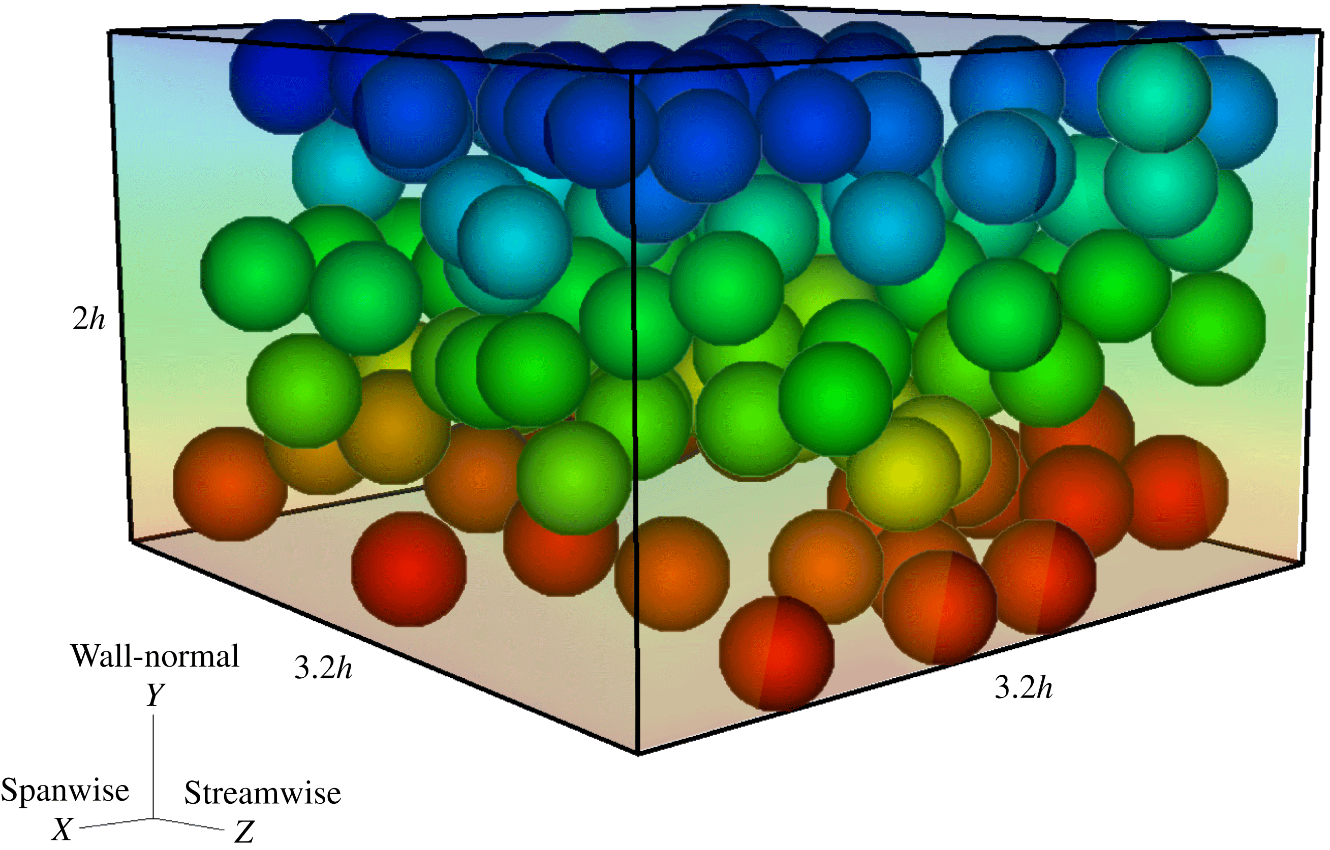
Figure 1. Instantaneous snapshot of the particle arrangement for a laminar shear thinning flow,
 $\dot{\unicode[STIX]{x1D6FE}}=1$
,
$\dot{\unicode[STIX]{x1D6FE}}=1$
,
 $Re_{p}=0.2004$
and
$Re_{p}=0.2004$
and
 $\unicode[STIX]{x1D6F7}=0.21$
. The wall-normal, streamwise and spanwise coordinates and particle diameters are shown in their actual size. The particle diameter is equal to
$\unicode[STIX]{x1D6F7}=0.21$
. The wall-normal, streamwise and spanwise coordinates and particle diameters are shown in their actual size. The particle diameter is equal to
 $2h/5$
with
$2h/5$
with
 $h$
the half-channel width.
$h$
the half-channel width.
The motion of the rigid spherical particles is described by the Newton–Euler equations,
 $$\begin{eqnarray}\displaystyle \left.\begin{array}{@{}c@{}}\displaystyle m_{p}\frac{\text{d}\boldsymbol{U}_{c}^{p}}{\text{d}t}=\boldsymbol{F}_{p},\\ \displaystyle I_{p}\frac{\text{d}\pmb{\unicode[STIX]{x1D6FA}}_{c}^{p}}{\text{d}t}=\boldsymbol{T}_{p},\end{array}\right\} & & \displaystyle\end{eqnarray}$$
where
 $\boldsymbol{U}_{c}^{p}$
and
$\boldsymbol{U}_{c}^{p}$
and
 $\pmb{\unicode[STIX]{x1D6FA}}_{c}^{p}$
are the translational and angular velocity of the particle
$\pmb{\unicode[STIX]{x1D6FA}}_{c}^{p}$
are the translational and angular velocity of the particle
 $p$
, while
$p$
, while
 $m_{p}$
and
$m_{p}$
and
 $I_{p}$
are the mass and moment of inertia,
$I_{p}$
are the mass and moment of inertia,
 $2m_{p}a^{2}/5$
, of a sphere with radius
$2m_{p}a^{2}/5$
, of a sphere with radius
 $a$
.
$a$
.
 $\boldsymbol{F}_{p}$
and
$\boldsymbol{F}_{p}$
and
 $\boldsymbol{T}_{p}$
are the net force and momentum resulting from hydrodynamic and particle–particle interactions,
$\boldsymbol{T}_{p}$
are the net force and momentum resulting from hydrodynamic and particle–particle interactions,
 $$\begin{eqnarray}\displaystyle \left.\begin{array}{@{}c@{}}\displaystyle \boldsymbol{F}_{p}=\oint _{\unicode[STIX]{x2202}V_{p}}[-P\unicode[STIX]{x1D644}+\hat{\unicode[STIX]{x1D707}}(\boldsymbol{u})(\unicode[STIX]{x1D735}\boldsymbol{u}+\unicode[STIX]{x1D735}\boldsymbol{u}^{\text{T}})]\boldsymbol{\cdot }\boldsymbol{n}\,\text{d}S+\boldsymbol{F}_{c},\\ \displaystyle \boldsymbol{T}_{p}=\oint _{\unicode[STIX]{x2202}V_{p}}\boldsymbol{r}\times \{[-P\unicode[STIX]{x1D644}+\hat{\unicode[STIX]{x1D707}}(\boldsymbol{u})(\unicode[STIX]{x1D735}\boldsymbol{u}+\unicode[STIX]{x1D735}\boldsymbol{u}^{\text{T}})]\boldsymbol{\cdot }\boldsymbol{n}\}\,\text{d}S+\boldsymbol{T}_{c}.\end{array}\right\} & & \displaystyle\end{eqnarray}$$
In these equations
 $\unicode[STIX]{x2202}V_{p}$
represents the surface of the particles with outwards normal vector
$\unicode[STIX]{x2202}V_{p}$
represents the surface of the particles with outwards normal vector
 $\boldsymbol{n}$
and
$\boldsymbol{n}$
and
 $\unicode[STIX]{x1D644}$
the identity tensor. The radial distance from the centre to the surface of each particle is indicated by
$\unicode[STIX]{x1D644}$
the identity tensor. The radial distance from the centre to the surface of each particle is indicated by
 $\boldsymbol{r}$
. The force and torque,
$\boldsymbol{r}$
. The force and torque,
 $\boldsymbol{F}_{c}$
and
$\boldsymbol{F}_{c}$
and
 $\boldsymbol{T}_{c}$
, act on the particle as a result of particle–particle or particle–wall contacts. The no-slip and no-penetration boundary conditions on the surface of the particles are imposed by forcing the fluid velocity at each point on the surface of the particle,
$\boldsymbol{T}_{c}$
, act on the particle as a result of particle–particle or particle–wall contacts. The no-slip and no-penetration boundary conditions on the surface of the particles are imposed by forcing the fluid velocity at each point on the surface of the particle,
 $\boldsymbol{X}$
, to be equal to particle velocity at that point,
$\boldsymbol{X}$
, to be equal to particle velocity at that point,
 $\boldsymbol{u}(\boldsymbol{X})=\boldsymbol{U}^{p}(\boldsymbol{X})=\boldsymbol{U}_{c}^{p}+\pmb{\unicode[STIX]{x1D6FA}}_{c}^{p}\times \boldsymbol{r}$
. This condition is not imposed directly in the immersed boundary method used in the current study, but instead included via the body force
$\boldsymbol{u}(\boldsymbol{X})=\boldsymbol{U}^{p}(\boldsymbol{X})=\boldsymbol{U}_{c}^{p}+\pmb{\unicode[STIX]{x1D6FA}}_{c}^{p}\times \boldsymbol{r}$
. This condition is not imposed directly in the immersed boundary method used in the current study, but instead included via the body force
 $\boldsymbol{f}$
on the right-hand side of (2.1).
$\boldsymbol{f}$
on the right-hand side of (2.1).
2.1.1 Viscosity models
Several models have been developed to capture the inelastic behaviour of some non-Newtonian fluids such as polymeric solutions. In the current work, we employ the Carreau law to describe the behaviour of shear thinning (pseudoplastic) fluids. This model describes the fluid viscosity well enough for most engineering calculations (Bird, Armstrong & Hassanger Reference Bird, Armstrong and Hassanger1987). The model assumes an isotropic viscosity proportional to some power of the shear rate
 $\dot{\unicode[STIX]{x1D6FE}}$
(Morrison Reference Morrison2001),
$\dot{\unicode[STIX]{x1D6FE}}$
(Morrison Reference Morrison2001),
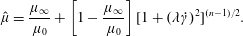 $$\begin{eqnarray}\hat{\unicode[STIX]{x1D707}}=\frac{\unicode[STIX]{x1D707}_{\infty }}{\unicode[STIX]{x1D707}_{0}}+\left[1-\frac{\unicode[STIX]{x1D707}_{\infty }}{\unicode[STIX]{x1D707}_{0}}\right][1+(\unicode[STIX]{x1D706}\dot{\unicode[STIX]{x1D6FE}})^{2}]^{(n-1)/2}.\end{eqnarray}$$
In the expression above
 $\hat{\unicode[STIX]{x1D707}}$
is the non-dimensional viscosity
$\hat{\unicode[STIX]{x1D707}}$
is the non-dimensional viscosity
 $\hat{\unicode[STIX]{x1D707}}=\unicode[STIX]{x1D707}/\unicode[STIX]{x1D707}_{0}$
, where
$\hat{\unicode[STIX]{x1D707}}=\unicode[STIX]{x1D707}/\unicode[STIX]{x1D707}_{0}$
, where
 $\unicode[STIX]{x1D707}_{0}$
is the zero shear rate viscosity. In this work the non-dimensional viscosity takes the value
$\unicode[STIX]{x1D707}_{0}$
is the zero shear rate viscosity. In this work the non-dimensional viscosity takes the value
 $\hat{\unicode[STIX]{x1D707}}=1$
at zero shear rate and
$\hat{\unicode[STIX]{x1D707}}=1$
at zero shear rate and
 $\hat{\unicode[STIX]{x1D707}}=\unicode[STIX]{x1D707}_{\infty }/\unicode[STIX]{x1D707}_{0}=0.001$
in the limit of infinite shear rate, as shown in figure 2(a). The second invariant of the strain-rate tensor
$\hat{\unicode[STIX]{x1D707}}=\unicode[STIX]{x1D707}_{\infty }/\unicode[STIX]{x1D707}_{0}=0.001$
in the limit of infinite shear rate, as shown in figure 2(a). The second invariant of the strain-rate tensor
 $\dot{\unicode[STIX]{x1D6FE}}$
is determined by the dyadic product of the strain tensor
$\dot{\unicode[STIX]{x1D6FE}}$
is determined by the dyadic product of the strain tensor
 $\dot{\unicode[STIX]{x1D6FE}}=\sqrt{2s_{ij}:s_{ij}}$
, where
$\dot{\unicode[STIX]{x1D6FE}}=\sqrt{2s_{ij}:s_{ij}}$
, where
 $\boldsymbol{s}=(\unicode[STIX]{x1D735}\boldsymbol{u}+\unicode[STIX]{x1D735}\boldsymbol{u}^{\text{T}})/2$
(see Bird et al.
Reference Bird, Armstrong and Hassanger1987). The power index
$\boldsymbol{s}=(\unicode[STIX]{x1D735}\boldsymbol{u}+\unicode[STIX]{x1D735}\boldsymbol{u}^{\text{T}})/2$
(see Bird et al.
Reference Bird, Armstrong and Hassanger1987). The power index
 $n$
indicates the non-Newtonian fluid behaviour. For
$n$
indicates the non-Newtonian fluid behaviour. For
 $n<1$
the fluid is shear thinning where the fluid viscosity decreases monotonically with the shear rate. The constant
$n<1$
the fluid is shear thinning where the fluid viscosity decreases monotonically with the shear rate. The constant
 $\unicode[STIX]{x1D706}$
is a dimensionless time, scaled by the flow time scale, and represents the degree of shear thinning. In the present study the power index and the time constant are fixed to
$\unicode[STIX]{x1D706}$
is a dimensionless time, scaled by the flow time scale, and represents the degree of shear thinning. In the present study the power index and the time constant are fixed to
 $n=0.3$
and
$n=0.3$
and
 $\unicode[STIX]{x1D706}=10$
. We report in figure 2(a), using markers, the range of shear rate and the corresponding viscosity of the carrier fluid used for the different simulations of particle-laden flows discussed later.
$\unicode[STIX]{x1D706}=10$
. We report in figure 2(a), using markers, the range of shear rate and the corresponding viscosity of the carrier fluid used for the different simulations of particle-laden flows discussed later.
For shear thickening (dilatant) fluid we employ the power-law model,
 $$\begin{eqnarray}\hat{\unicode[STIX]{x1D707}}=\hat{m}\dot{\unicode[STIX]{x1D6FE}}^{n-1},\end{eqnarray}$$
which reproduces a monotonic increase of the viscosity with the local shear rate when
 $n>1$
. The constant
$n>1$
. The constant
 $\hat{m}$
is called the consistency index and indicates the slope of the viscosity profile. For a shear thickening fluid we use
$\hat{m}$
is called the consistency index and indicates the slope of the viscosity profile. For a shear thickening fluid we use
 $n=1.5$
and
$n=1.5$
and
 $\hat{m}=1$
. This corresponds to
$\hat{m}=1$
. This corresponds to
 $\hat{\unicode[STIX]{x1D707}}=1$
at the lowest shear rate employed in the study, see figure 2(b). For a more detailed description of the parameters appearing in the Carreau- and power-law models we refer the readers to the book by Morrison (Reference Morrison2001).
$\hat{\unicode[STIX]{x1D707}}=1$
at the lowest shear rate employed in the study, see figure 2(b). For a more detailed description of the parameters appearing in the Carreau- and power-law models we refer the readers to the book by Morrison (Reference Morrison2001).
Figure 2. The non-dimensional fluid viscosity
 $\hat{\unicode[STIX]{x1D707}}$
versus shear rate
$\hat{\unicode[STIX]{x1D707}}$
versus shear rate
 $\dot{\unicode[STIX]{x1D6FE}}$
for (a) Newtonian, (b) Carreau-law model (shear thinning) with
$\dot{\unicode[STIX]{x1D6FE}}$
for (a) Newtonian, (b) Carreau-law model (shear thinning) with
 $n=0.3$
,
$n=0.3$
,
 $\unicode[STIX]{x1D706}=10$
and (c) power-law model (shear thickening) for
$\unicode[STIX]{x1D706}=10$
and (c) power-law model (shear thickening) for
 $n=1.5$
. The markers shows the shear rates and viscosities of the carrier fluid for the different cases considered here.
$n=1.5$
. The markers shows the shear rates and viscosities of the carrier fluid for the different cases considered here.
2.2 Numerical method
The particle motion in the flow is simulated by means of an efficient immersed boundary method (IBM) coupled with a flow solver for the generalised Navier–Stokes equations. We follow the formulation by Breugem (Reference Breugem2012) developed to increase the numerical accuracy and stability for simulations of neutrally buoyant particles.
The governing equations for the fluid phase are discretised using a second-order central difference scheme; the Crank–Nicholson scheme is used for the time integration of the viscous term while the nonlinear term is treated explicitly using the three-step Runge–Kutta scheme. A fixed and staggered Eulerian grid is used for the fluid phase whereas a Lagrangian grid is attached to the surface of each particle. These two grid points communicate via the IBM forcing to satisfy the no-slip and no-penetration boundary conditions on the surface of the particles.
The interactions between the particles and/or wall are taken into account using the lubrication correction and soft collision model described in detail in Costa et al. (Reference Costa, Boersma, Westerweel and Breugem2015). When the gap distance between the particle–particle or particle–wall becomes smaller than a certain threshold, a mesh dependent lubrication correction based on the asymptotic solution by Brenner (Reference Brenner1961) is employed to reproduce correctly the interaction between the particles. At smaller gaps the lubrication correction is kept constant to account for the surface roughness. Finally, a soft-sphere collision model is activated based on the relative velocity and the overlap between the two particles (particle–wall), where both the normal and tangential components of the contact force are taken into account. The accuracy of the IBM code is examined extensively in the work by Breugem (Reference Breugem2012), Lambert et al. (Reference Lambert, Picano, Breugem and Brandt2013), Costa et al. (Reference Costa, Boersma, Westerweel and Breugem2015), Picano et al. (Reference Picano, Breugem and Brandt2015), among others. One issue with the IBM scheme is the fluid trapped inside of the particles. Although, the effect of the fluid acceleration inside the particles is accounted for and subtracted from the forces acting on the particle, it can still result in non-realistic values of the local shear rate for the grid points close to the interface. To fix this issue, a volume of fluid scheme is used to create a velocity field that replaces the velocity of the fluid inside the particles with their rigid body motion. At the interface (the surface of the particles), a weighted average of solid and fluid velocities is considered based on the local solid volume fraction of the Eulerian grid in this region.
Another issue concerns the use of the lubrication correction as suggested in the original IBM method of Breugem (Reference Breugem2012) for Newtonian fluids. To extend this model to non-Newtonian fluids and approximate the lubrication correction force when particles are less than one grid cell away from each other, we use in the asymptotic solution by Brenner (Reference Brenner1961) the local viscosity at the Eulerian point closest to the mid-point of the line connecting the centres of two particles in interaction. It is noteworthy to mention that the viscosity is calculated explicitly from the local shear rate, using the velocities from the previous substep of the Runge–Kutta time integration scheme. As regards the implementation of the viscosity model in our solver, we have tested the code for the unladen channel flow of shear-dependent viscosity fluids against the analytical solution, see Nouar, Bottaro & Brancher (Reference Nouar, Bottaro and Brancher2007). Figure 3 shows a typical example of this validation.

Figure 3. The velocity profiles of generalised Newtonian fluids flowing in a channel. The boundary conditions and configuration are similar to those of figure 1. The pressure drop is implemented as a source term to give a bulk Reynolds number of 100. Solid lines: the theoretical prediction. Symbols: the simulation results.
2.3 Flow configuration and numerical set-up
In this study, we perform interface-resolved simulations of suspensions of neutrally buoyant spheres in shear thinning and shear thickening fluids. The flow is driven by the motion of the upper and lower walls in a plane Couette configuration. Periodic boundary conditions are imposed in the streamwise and spanwise directions. Similar to Picano et al. (Reference Picano, Breugem, Mitra and Brandt2013), we use a box size of
 $2h\times 3.2h\times 3.2h$
with
$2h\times 3.2h\times 3.2h$
with
 $h$
the half-channel width; the number of uniform Eulerian grid points is
$h$
the half-channel width; the number of uniform Eulerian grid points is
 $80\times 128\times 128$
in the wall-normal, streamwise and spanwise directions. The particles have all the same radius,
$80\times 128\times 128$
in the wall-normal, streamwise and spanwise directions. The particles have all the same radius,
 $a=h/5$
, which corresponds to 8 Eulerian grid points per particle radius, whereas 746 Lagrangian grid points are used on the surface of each particle to resolve the fluid–particle interactions. The fluid is sheared in the
$a=h/5$
, which corresponds to 8 Eulerian grid points per particle radius, whereas 746 Lagrangian grid points are used on the surface of each particle to resolve the fluid–particle interactions. The fluid is sheared in the
 $y$
–
$y$
–
 $z$
plane by imposing a constant streamwise velocity of opposite sign
$z$
plane by imposing a constant streamwise velocity of opposite sign
 $V_{w}=\dot{\unicode[STIX]{x1D6FE}}h$
at the two horizontal walls.
$V_{w}=\dot{\unicode[STIX]{x1D6FE}}h$
at the two horizontal walls.
In this work we fix the rheological parameters and vary the wall velocity (the shear rate
 $\dot{\unicode[STIX]{x1D6FE}}$
) and the particle volume fraction
$\dot{\unicode[STIX]{x1D6FE}}$
) and the particle volume fraction
 $\unicode[STIX]{x1D6F7}$
. We explore a wide range of shear rates,
$\unicode[STIX]{x1D6F7}$
. We explore a wide range of shear rates,
 $0.1\leqslant \dot{\unicode[STIX]{x1D6FE}}\leqslant 10$
, corresponding to the particle Reynolds numbers
$0.1\leqslant \dot{\unicode[STIX]{x1D6FE}}\leqslant 10$
, corresponding to the particle Reynolds numbers
 $0.1\leqslant Re_{p}=\unicode[STIX]{x1D70C}\dot{\unicode[STIX]{x1D6FE}}a^{2}/\unicode[STIX]{x1D707}\leqslant 10$
for the Newtonian fluid,
$0.1\leqslant Re_{p}=\unicode[STIX]{x1D70C}\dot{\unicode[STIX]{x1D6FE}}a^{2}/\unicode[STIX]{x1D707}\leqslant 10$
for the Newtonian fluid,
 $0.5\leqslant \dot{\unicode[STIX]{x1D6FE}}\leqslant 10$
corresponding to
$0.5\leqslant \dot{\unicode[STIX]{x1D6FE}}\leqslant 10$
corresponding to
 $0.0624\leqslant Re_{p}\leqslant 9.8113$
for the shear thinning fluid and
$0.0624\leqslant Re_{p}\leqslant 9.8113$
for the shear thinning fluid and
 $1\leqslant \dot{\unicode[STIX]{x1D6FE}}\leqslant 10\,000$
corresponding to
$1\leqslant \dot{\unicode[STIX]{x1D6FE}}\leqslant 10\,000$
corresponding to
 $0.1\leqslant Re_{p}\leqslant 10$
for the shear thickening fluid, see figure 2. Note that
$0.1\leqslant Re_{p}\leqslant 10$
for the shear thickening fluid, see figure 2. Note that
 $\unicode[STIX]{x1D707}$
in the definition of the particle Reynolds number is, for each case, the non-Newtonian fluid viscosity in the absence of particles. For each suspending fluid, (Newtonian, shear thinning or shear thickening fluid), the range of shear rate as well as the values of zero shear rate viscosities are chosen such that we cover the same range of particle Reynolds number, i.e.
$\unicode[STIX]{x1D707}$
in the definition of the particle Reynolds number is, for each case, the non-Newtonian fluid viscosity in the absence of particles. For each suspending fluid, (Newtonian, shear thinning or shear thickening fluid), the range of shear rate as well as the values of zero shear rate viscosities are chosen such that we cover the same range of particle Reynolds number, i.e.
 $0.1\leqslant Re_{p}\leqslant 10$
. Four different particle volume fractions,
$0.1\leqslant Re_{p}\leqslant 10$
. Four different particle volume fractions,
 $\unicode[STIX]{x1D6F7}=0.11,0.21,0.315$
and
$\unicode[STIX]{x1D6F7}=0.11,0.21,0.315$
and
 $0.4$
, are examined; this corresponds to
$0.4$
, are examined; this corresponds to
 $N_{p}=67,128,193$
and
$N_{p}=67,128,193$
and
 $245$
particles in the simulation domain. The particles are initialised randomly in the channel with velocities equal to the local velocity of the laminar Couette profile. The parameters of the different simulations are summarised in table 1. Results are collected after the flow reaches a statistically steady state. We ensure the convergence by repeating the analysis using half the number of samples and comparing the statistics with those from the entire number of samples.
$245$
particles in the simulation domain. The particles are initialised randomly in the channel with velocities equal to the local velocity of the laminar Couette profile. The parameters of the different simulations are summarised in table 1. Results are collected after the flow reaches a statistically steady state. We ensure the convergence by repeating the analysis using half the number of samples and comparing the statistics with those from the entire number of samples.

Figure 4. Wall-normal profiles of the local particle volume fraction for (a)
 $Re_{p}=0.1$
; (b)
$Re_{p}=0.1$
; (b)
 $Re_{p}=6$
. The following colours are adopted for suspensions with different types of suspending fluids: the Newtonian suspending fluids: red colour; the shear thinning suspending fluid: black colour and the shear thickening suspending fluid: blue colour. The following symbols are adopted for different solid volume fractions:
$Re_{p}=6$
. The following colours are adopted for suspensions with different types of suspending fluids: the Newtonian suspending fluids: red colour; the shear thinning suspending fluid: black colour and the shear thickening suspending fluid: blue colour. The following symbols are adopted for different solid volume fractions:
 $\unicode[STIX]{x1D6F7}=0.11$
: ▫;
$\unicode[STIX]{x1D6F7}=0.11$
: ▫;
 $\unicode[STIX]{x1D6F7}=0.21$
: ○;
$\unicode[STIX]{x1D6F7}=0.21$
: ○;
 $\unicode[STIX]{x1D6F7}=0.315$
: ▵ and
$\unicode[STIX]{x1D6F7}=0.315$
: ▵ and
 $\unicode[STIX]{x1D6F7}=0.40$
:
$\unicode[STIX]{x1D6F7}=0.40$
:
 $\star$
.
$\star$
.
3 Results
In the present study, we investigate the flow of rigid particles in a simple shear where the carrier fluid is Newtonian, shear thinning or shear thickening. We focus on the bulk properties of the suspension as well as its local behaviour. We present the distribution of particle and fluid phase velocity, particle volume fraction and local shear rate. Then we study the rheology of these suspensions and compare our results with predictions from the homogenisation theory presented by Chateau et al. (Reference Chateau, Ovarlez and Trung2008), valid for Stokesian suspensions. We therefore focus on how inertia affects the suspension behaviour.
Table 1. Summary of the simulations performed.
 $Re_{p,local}(\unicode[STIX]{x1D6F7}(\%))$
is the local particle Reynolds number for different values of
$Re_{p,local}(\unicode[STIX]{x1D6F7}(\%))$
is the local particle Reynolds number for different values of
 $\unicode[STIX]{x1D6F7}$
and
$\unicode[STIX]{x1D6F7}$
and
 $\bar{\dot{\unicode[STIX]{x1D6FE}}}_{local}$
.
$\bar{\dot{\unicode[STIX]{x1D6FE}}}_{local}$
.

3.1 Flow profiles
The wall-normal profiles of the local particle volume fraction
 $\unicode[STIX]{x1D6F7}(y)$
are computed for all the simulations listed in table 1 by averaging the local solid volume fraction over time and in the spanwise direction. A typical example of the results is shown in figure 4. Here the wall-normal distribution of
$\unicode[STIX]{x1D6F7}(y)$
are computed for all the simulations listed in table 1 by averaging the local solid volume fraction over time and in the spanwise direction. A typical example of the results is shown in figure 4. Here the wall-normal distribution of
 $\unicode[STIX]{x1D6F7}(y)$
is displayed across half of the gap for four particle volume fractions,
$\unicode[STIX]{x1D6F7}(y)$
is displayed across half of the gap for four particle volume fractions,
 $\unicode[STIX]{x1D6F7}=[0.11,0.21,0.315,0.4]$
, and two particle Reynolds numbers
$\unicode[STIX]{x1D6F7}=[0.11,0.21,0.315,0.4]$
, and two particle Reynolds numbers
 $Re_{p}=[0.1,6]$
for Newtonian, shear thinning and shear thickening suspending fluids. Three features are evident here. First, particles tend to form layers due to the wall confinement; the number of particles at the wall is larger than in the bulk. Second, the particle layering increases as the bulk solid volume fraction increases. Third, the distribution of
$Re_{p}=[0.1,6]$
for Newtonian, shear thinning and shear thickening suspending fluids. Three features are evident here. First, particles tend to form layers due to the wall confinement; the number of particles at the wall is larger than in the bulk. Second, the particle layering increases as the bulk solid volume fraction increases. Third, the distribution of
 $\unicode[STIX]{x1D6F7}(y)$
changes slightly with the type of suspending fluid over the range of the particle Reynolds number studied here (i.e.
$\unicode[STIX]{x1D6F7}(y)$
changes slightly with the type of suspending fluid over the range of the particle Reynolds number studied here (i.e.
 $0<Re_{p}\leqslant 10$
), suggesting that the local particle volume fraction is mainly controlled by geometry and confinement. A detailed study of confinement is beyond the scope of this manuscript. However, more recent results to be published elsewhere show that decreasing confinement by
$0<Re_{p}\leqslant 10$
), suggesting that the local particle volume fraction is mainly controlled by geometry and confinement. A detailed study of confinement is beyond the scope of this manuscript. However, more recent results to be published elsewhere show that decreasing confinement by
 $50\,\%$
when dealing with oblate particles has a less than
$50\,\%$
when dealing with oblate particles has a less than
 $1\,\%$
effect on the bulk rheology.
$1\,\%$
effect on the bulk rheology.

Figure 5. Wall-normal profiles of the normalised mean fluid streamwise velocity,
 $V_{f}/V_{w}$
: (a)
$V_{f}/V_{w}$
: (a)
 $Re_{p}=0.1$
; (b)
$Re_{p}=0.1$
; (b)
 $Re_{p}=6$
. The normalised mean particle streamwise velocity,
$Re_{p}=6$
. The normalised mean particle streamwise velocity,
 $V_{p}/V_{w}$
: (c)
$V_{p}/V_{w}$
: (c)
 $Re_{p}=0.1$
; (d)
$Re_{p}=0.1$
; (d)
 $Re_{p}=6$
. The following colours are adopted for suspensions with different type of suspending fluids: the Newtonian suspending fluids: red colour; the shear thinning suspending fluid: black colour and the shear thickening suspending fluid: blue colour. The following symbols are adopted for different solid volume fractions:
$Re_{p}=6$
. The following colours are adopted for suspensions with different type of suspending fluids: the Newtonian suspending fluids: red colour; the shear thinning suspending fluid: black colour and the shear thickening suspending fluid: blue colour. The following symbols are adopted for different solid volume fractions:
 $\unicode[STIX]{x1D6F7}=0.11$
: ▫;
$\unicode[STIX]{x1D6F7}=0.11$
: ▫;
 $\unicode[STIX]{x1D6F7}=0.21$
: ○;
$\unicode[STIX]{x1D6F7}=0.21$
: ○;
 $\unicode[STIX]{x1D6F7}=0.315$
: ▵ and
$\unicode[STIX]{x1D6F7}=0.315$
: ▵ and
 $\unicode[STIX]{x1D6F7}=0.40$
:
$\unicode[STIX]{x1D6F7}=0.40$
:
 $\star$
.
$\star$
.
We report the normalised mean fluid
 $V_{f}/V_{w}$
and particle velocity
$V_{f}/V_{w}$
and particle velocity
 $V_{p}/V_{w}$
in figure 5 for the same values of the particle Reynolds number and bulk solid volume fraction in figure 4, using the same symbol and colour scheme throughout the manuscript. The statistics of the fluid phase velocity have been computed neglecting the points occupied by the solid phase in each field (phase-ensemble average). Generally, independent of the type of suspending fluid, the normalised mean fluid velocity decreases in the intermediate region between the wall and the centreline,
$V_{p}/V_{w}$
in figure 5 for the same values of the particle Reynolds number and bulk solid volume fraction in figure 4, using the same symbol and colour scheme throughout the manuscript. The statistics of the fluid phase velocity have been computed neglecting the points occupied by the solid phase in each field (phase-ensemble average). Generally, independent of the type of suspending fluid, the normalised mean fluid velocity decreases in the intermediate region between the wall and the centreline,
 $0.02\lesssim y/h\lesssim 0.4$
as the particle volume fraction
$0.02\lesssim y/h\lesssim 0.4$
as the particle volume fraction
 $\unicode[STIX]{x1D6F7}$
and shear rate or
$\unicode[STIX]{x1D6F7}$
and shear rate or
 $Re_{p}$
increase. The larger differences between the different cases are found close to the wall. The deviation of the normalised mean fluid velocity profile from linearity is more pronounced for the shear thinning suspending fluid and less evident for the shear thickening fluid. This is due to the fact that the local viscosity seen by the particles in the case of generalised Newtonian fluids depends on the local shear rate. Taking this into account results in larger and smaller local particle Reynolds numbers for the shear thinning and shear thickening fluids, respectively (see § 3.2 for more details). The values of the local particle Reynolds number (see (3.7)) are reported in table 1.
$Re_{p}$
increase. The larger differences between the different cases are found close to the wall. The deviation of the normalised mean fluid velocity profile from linearity is more pronounced for the shear thinning suspending fluid and less evident for the shear thickening fluid. This is due to the fact that the local viscosity seen by the particles in the case of generalised Newtonian fluids depends on the local shear rate. Taking this into account results in larger and smaller local particle Reynolds numbers for the shear thinning and shear thickening fluids, respectively (see § 3.2 for more details). The values of the local particle Reynolds number (see (3.7)) are reported in table 1.
The statistics pertaining to the solid phase, depicted in figure 5(c,d), are calculated using quantities related to each individual particle, and taking the phase-ensemble average over time and space. As for the carrier fluid, the normalised mean particle velocity decreases when increasing the volume fraction
 $\unicode[STIX]{x1D6F7}$
and inertial effects,
$\unicode[STIX]{x1D6F7}$
and inertial effects,
 $Re_{p}$
. Again this is more significant for the case of shear thinning suspending fluid due to the smaller apparent viscosity at the particle scale (or equivalently the larger local particle Reynolds number). Moreover, comparing figures 5(a) and 5(c) (and similarly figures 5
b and 5
d), we note that the slip velocity between the solid phase and fluid phase increases close to the wall. In particular, particles move faster close to the walls,
$Re_{p}$
. Again this is more significant for the case of shear thinning suspending fluid due to the smaller apparent viscosity at the particle scale (or equivalently the larger local particle Reynolds number). Moreover, comparing figures 5(a) and 5(c) (and similarly figures 5
b and 5
d), we note that the slip velocity between the solid phase and fluid phase increases close to the wall. In particular, particles move faster close to the walls,
 $y/h\lesssim 0.2$
, something explained by the different boundary conditions (particles can roll and slide on the wall). This slip is more evident for the case of a shear thinning suspending fluid, suggesting that as we increase the local particle Reynolds number, any modelling would need to take into account a boundary layer close to the wall governed by a two-phase equation of motion instead of mixture equations (Dontsov & Peirce Reference Dontsov and Peirce2014; Costa et al.
Reference Costa, Picano, Brandt and Breugem2016). Indeed, continuum models are more prone to failure when the slip velocity between fluid and particles is not negligible, i.e. the particle Stokes number is large.
$y/h\lesssim 0.2$
, something explained by the different boundary conditions (particles can roll and slide on the wall). This slip is more evident for the case of a shear thinning suspending fluid, suggesting that as we increase the local particle Reynolds number, any modelling would need to take into account a boundary layer close to the wall governed by a two-phase equation of motion instead of mixture equations (Dontsov & Peirce Reference Dontsov and Peirce2014; Costa et al.
Reference Costa, Picano, Brandt and Breugem2016). Indeed, continuum models are more prone to failure when the slip velocity between fluid and particles is not negligible, i.e. the particle Stokes number is large.
3.2 Stokesian rheology: homogenisation approach
In this section, we briefly explain the theoretical prediction for the rheology of an inertialess suspension of rigid spherical particles in generalised Newtonian fluids. This theoretical approach is based on homogenisation theory and was first developed by Chateau et al. (Reference Chateau, Ovarlez and Trung2008) assuming isotropic suspensions. Later, Ovarlez et al. (Reference Ovarlez, Mahaut, Deboeufg, Lenoir, Hormozi and Chateau2015), Dagois-Bohy et al. (Reference Dagois-Bohy, Hormozi, Guazzelli and Pouliquen2015) and Hormozi & Frigaard (Reference Hormozi and Frigaard2017) extended this theory to estimate the rheology of anisotropic dilute and dense suspensions.
In order to predict the rheology of the suspensions we need to know the value of the local shear rate
 $\dot{\unicode[STIX]{x1D6FE}}_{local}(x,y,z)$
for a bulk shear rate
$\dot{\unicode[STIX]{x1D6FE}}_{local}(x,y,z)$
for a bulk shear rate
 $\dot{\unicode[STIX]{x1D6FE}}$
. In homogenisation theory, it is assumed that the bulk rheology is determined by the mean value of the local shear rate, i.e.
$\dot{\unicode[STIX]{x1D6FE}}$
. In homogenisation theory, it is assumed that the bulk rheology is determined by the mean value of the local shear rate, i.e.
 $\bar{\dot{\unicode[STIX]{x1D6FE}}}_{local}$
. Following Chateau et al. (Reference Chateau, Ovarlez and Trung2008), we assume that viscous dissipation is responsible for the entire energy loss in the suspension (Chateau et al.
Reference Chateau, Ovarlez and Trung2008; DeGiuli et al.
Reference DeGiuli, Düring, Lerner and Wyart2015). This gives the following estimate for the mean local shear rate
$\bar{\dot{\unicode[STIX]{x1D6FE}}}_{local}$
. Following Chateau et al. (Reference Chateau, Ovarlez and Trung2008), we assume that viscous dissipation is responsible for the entire energy loss in the suspension (Chateau et al.
Reference Chateau, Ovarlez and Trung2008; DeGiuli et al.
Reference DeGiuli, Düring, Lerner and Wyart2015). This gives the following estimate for the mean local shear rate
 $$\begin{eqnarray}\displaystyle & \displaystyle \bar{\dot{\unicode[STIX]{x1D6FE}}}_{local}(\unicode[STIX]{x1D6F7})=\sqrt{\langle \dot{\unicode[STIX]{x1D6FE}}_{local}^{2}(x,y,z)\rangle }=\dot{\unicode[STIX]{x1D6FE}}\sqrt{\frac{G(\unicode[STIX]{x1D6F7})}{1-\unicode[STIX]{x1D6F7}}}, & \displaystyle\end{eqnarray}$$
 $$\begin{eqnarray}\displaystyle & \displaystyle G(\unicode[STIX]{x1D6F7})=\left[1+B\frac{\unicode[STIX]{x1D6F7}}{1-\unicode[STIX]{x1D6F7}/\unicode[STIX]{x1D6F7}_{max}}\right]^{2}, & \displaystyle\end{eqnarray}$$
where
 $\langle \cdot \rangle$
denotes the average of a quantity over the whole domain and
$\langle \cdot \rangle$
denotes the average of a quantity over the whole domain and
 $G(\unicode[STIX]{x1D6F7})$
is the dimensionless relative shear viscosity. The latter, a sole function of the particle volume fraction, increases monotonically with
$G(\unicode[STIX]{x1D6F7})$
is the dimensionless relative shear viscosity. The latter, a sole function of the particle volume fraction, increases monotonically with
 $\unicode[STIX]{x1D6F7}$
and diverges when jamming occurs at the maximum packing fraction,
$\unicode[STIX]{x1D6F7}$
and diverges when jamming occurs at the maximum packing fraction,
 $\unicode[STIX]{x1D6F7}_{max}$
. For non-dilute non-colloidal suspensions various empirical fits to the experimental data have been proposed (Maron & Pierce Reference Maron and Pierce1956; Krieger & Dougherty Reference Krieger and Dougherty1959; Quemada Reference Quemada1977; Mendoza & Santamaria-Holek Reference Mendoza and Santamaria-Holek2009). In this work we use Eilers fit (Stickel & Powell Reference Stickel and Powell2005), where
$\unicode[STIX]{x1D6F7}_{max}$
. For non-dilute non-colloidal suspensions various empirical fits to the experimental data have been proposed (Maron & Pierce Reference Maron and Pierce1956; Krieger & Dougherty Reference Krieger and Dougherty1959; Quemada Reference Quemada1977; Mendoza & Santamaria-Holek Reference Mendoza and Santamaria-Holek2009). In this work we use Eilers fit (Stickel & Powell Reference Stickel and Powell2005), where
 $B=1.25{-}1.5$
and the maximum packing fraction
$B=1.25{-}1.5$
and the maximum packing fraction
 $\unicode[STIX]{x1D6F7}_{max}=0.58{-}0.64$
(Zarraga et al.
Reference Zarraga, Hill and Leighton2000; Singh & Nott Reference Singh and Nott2003; Kulkarni & Morris Reference Kulkarni and Morris2008; Shewan & Stokes Reference Shewan and Stokes2015). The precise choice of the values for those parameters depend on particle shape, size, concentration and the shear rate (Konijn, Sanderink & Kruyt Reference Konijn, Sanderink and Kruyt2014). The values used here are
$\unicode[STIX]{x1D6F7}_{max}=0.58{-}0.64$
(Zarraga et al.
Reference Zarraga, Hill and Leighton2000; Singh & Nott Reference Singh and Nott2003; Kulkarni & Morris Reference Kulkarni and Morris2008; Shewan & Stokes Reference Shewan and Stokes2015). The precise choice of the values for those parameters depend on particle shape, size, concentration and the shear rate (Konijn, Sanderink & Kruyt Reference Konijn, Sanderink and Kruyt2014). The values used here are
 $B=1.5$
and
$B=1.5$
and
 $\unicode[STIX]{x1D6F7}_{max}=0.61$
.
$\unicode[STIX]{x1D6F7}_{max}=0.61$
.
The apparent viscosity of the suspending fluid can be estimated via a linearisation of the fluid behaviour at each imposed shear rate, similar to (2.4) and (2.5) for power-law and Carreau suspending fluids. We assume that the same relative viscosity as in Newtonian suspensions can be adopted when the suspending fluid is non-Newtonian. Therefore, the shear stress of the suspension can be written as
 $$\begin{eqnarray}\unicode[STIX]{x1D70F}_{ij}=G(\unicode[STIX]{x1D6F7})\unicode[STIX]{x1D707}_{0}\hat{\unicode[STIX]{x1D707}}\dot{\unicode[STIX]{x1D6FE}}_{ij},\end{eqnarray}$$
where
 $\hat{\unicode[STIX]{x1D707}}$
is the dimensionless apparent viscosity seen by the particles; this depends on the local shear rate that we estimate by its mean value
$\hat{\unicode[STIX]{x1D707}}$
is the dimensionless apparent viscosity seen by the particles; this depends on the local shear rate that we estimate by its mean value
 $\bar{\dot{\unicode[STIX]{x1D6FE}}}_{local}(\unicode[STIX]{x1D6F7})$
.
$\bar{\dot{\unicode[STIX]{x1D6FE}}}_{local}(\unicode[STIX]{x1D6F7})$
.
 $\hat{\unicode[STIX]{x1D707}}$
is of the following form for the Carreau and power-law suspending fluids considered in this work
$\hat{\unicode[STIX]{x1D707}}$
is of the following form for the Carreau and power-law suspending fluids considered in this work
 $$\begin{eqnarray}\displaystyle & \displaystyle \hat{\unicode[STIX]{x1D707}}(\bar{\dot{\unicode[STIX]{x1D6FE}}}_{local}(\unicode[STIX]{x1D6F7}))=\frac{\unicode[STIX]{x1D707}_{\infty }}{\unicode[STIX]{x1D707}_{0}}+\left[1-\frac{\unicode[STIX]{x1D707}_{\infty }}{\unicode[STIX]{x1D707}_{0}}\right][1+(\unicode[STIX]{x1D706}^{2}\bar{\dot{\unicode[STIX]{x1D6FE}}}_{local}^{2}(\unicode[STIX]{x1D6F7}))]^{(n-1)/2}, & \displaystyle\end{eqnarray}$$
 $$\begin{eqnarray}\displaystyle & \displaystyle \hat{\unicode[STIX]{x1D707}}(\bar{\dot{\unicode[STIX]{x1D6FE}}}_{local}(\unicode[STIX]{x1D6F7}))=\hat{m}\bar{\dot{\unicode[STIX]{x1D6FE}}}_{local}^{n-1}(\unicode[STIX]{x1D6F7}). & \displaystyle\end{eqnarray}$$
We can define the following apparent viscosity seen by the particles
 $$\begin{eqnarray}\unicode[STIX]{x1D707}_{f}(\bar{\dot{\unicode[STIX]{x1D6FE}}}_{local})=\unicode[STIX]{x1D707}_{0}\hat{\unicode[STIX]{x1D707}}(\bar{\dot{\unicode[STIX]{x1D6FE}}}_{local}(\unicode[STIX]{x1D6F7})),\end{eqnarray}$$
and consequently a local particle Reynolds number as follows
 $$\begin{eqnarray}Re_{p,local}=\frac{\unicode[STIX]{x1D70C}_{f}a^{2}\dot{\unicode[STIX]{x1D6FE}}}{\unicode[STIX]{x1D707}_{f}(\bar{\dot{\unicode[STIX]{x1D6FE}}}_{local})}.\end{eqnarray}$$
Finally, we may write the overall expression for the bulk effective viscosity of the suspension as follows
 $$\begin{eqnarray}\unicode[STIX]{x1D707}_{eff}(\unicode[STIX]{x1D6F7},\dot{\unicode[STIX]{x1D6FE}})=G(\unicode[STIX]{x1D6F7})\unicode[STIX]{x1D707}_{0}\hat{\unicode[STIX]{x1D707}}(\bar{\dot{\unicode[STIX]{x1D6FE}}}_{local}(\unicode[STIX]{x1D6F7})).\end{eqnarray}$$
We substitute for the local shear rate from (3.1) into (3.4) and (3.5), considering the definition of the suspension effective viscosity (3.8) to obtain the following dimensionless rheological formulation of the effective viscosity for shear thinning Carreau-law model) and shear thickening (power-law) fluids
 $$\begin{eqnarray}\displaystyle & \displaystyle \hat{\unicode[STIX]{x1D707}}_{eff}(\unicode[STIX]{x1D6F7},\dot{\unicode[STIX]{x1D6FE}})=G(\unicode[STIX]{x1D6F7})\left(\frac{\unicode[STIX]{x1D707}_{\infty }}{\unicode[STIX]{x1D707}_{0}}+\left[1-\frac{\unicode[STIX]{x1D707}_{\infty }}{\unicode[STIX]{x1D707}_{0}}\right]\left[1+(\unicode[STIX]{x1D706}\dot{\unicode[STIX]{x1D6FE}})^{2}\left(\frac{G(\unicode[STIX]{x1D6F7})}{1-\unicode[STIX]{x1D6F7}}\right)\right]^{(n-1)/2}\right), & \displaystyle\end{eqnarray}$$
 $$\begin{eqnarray}\displaystyle & \displaystyle \hat{\unicode[STIX]{x1D707}}_{eff}(\unicode[STIX]{x1D6F7},\dot{\unicode[STIX]{x1D6FE}})=G(\unicode[STIX]{x1D6F7})\hat{m}(\dot{\unicode[STIX]{x1D6FE}})^{n-1}\left(\frac{G(\unicode[STIX]{x1D6F7})}{1-\unicode[STIX]{x1D6F7}}\right)^{(n-1)/2}. & \displaystyle\end{eqnarray}$$
It is noteworthy to mention that the above framework is developed for Stokesian suspensions. Also,
 $G(\unicode[STIX]{x1D6F7})$
includes all the information about the microstructure of the suspensions which might not be independent of the shear rate for the case of generalised Newtonian suspending fluids. We therefore investigate these assumptions by means of numerical simulations. One of our goals is to shed light on the recent experimental results in the Stokesian regime by Madraki et al. (Reference Madraki, Hormozi, Ovarlez, Guazzelli and Pouliquen2017) that show discrepancies with the homogenisation predictions. Moreover, we will show how inertia affects the rheology,
$G(\unicode[STIX]{x1D6F7})$
includes all the information about the microstructure of the suspensions which might not be independent of the shear rate for the case of generalised Newtonian suspending fluids. We therefore investigate these assumptions by means of numerical simulations. One of our goals is to shed light on the recent experimental results in the Stokesian regime by Madraki et al. (Reference Madraki, Hormozi, Ovarlez, Guazzelli and Pouliquen2017) that show discrepancies with the homogenisation predictions. Moreover, we will show how inertia affects the rheology,
 $G(\unicode[STIX]{x1D6F7})$
, and provide a stress closure for non-colloidal suspensions in the presence of inertia.
$G(\unicode[STIX]{x1D6F7})$
, and provide a stress closure for non-colloidal suspensions in the presence of inertia.

Figure 6. Profiles of the probability distribution function (PDF) of the normalised local shear rate,
 $\dot{\unicode[STIX]{x1D6FE}}_{local}^{2}(x,y,z)/\dot{\unicode[STIX]{x1D6FE}}^{2}$
, for: (a)
$\dot{\unicode[STIX]{x1D6FE}}_{local}^{2}(x,y,z)/\dot{\unicode[STIX]{x1D6FE}}^{2}$
, for: (a)
 $Re_{p}=0.1$
; (b)
$Re_{p}=0.1$
; (b)
 $Re_{p}=6$
. Colours and symbols as in previous figures.
$Re_{p}=6$
. Colours and symbols as in previous figures.

Figure 7. Simulation results of (a)
 $\bar{\dot{\unicode[STIX]{x1D6FE}}}_{local}^{2}/\dot{\unicode[STIX]{x1D6FE}}^{2}$
; (b) normalised standard deviation
$\bar{\dot{\unicode[STIX]{x1D6FE}}}_{local}^{2}/\dot{\unicode[STIX]{x1D6FE}}^{2}$
; (b) normalised standard deviation
 $SD/\dot{\unicode[STIX]{x1D6FE}}^{2}$
, versus
$SD/\dot{\unicode[STIX]{x1D6FE}}^{2}$
, versus
 $Re_{p}$
. Colours and symbols as in previous figures.
$Re_{p}$
. Colours and symbols as in previous figures.
3.3 Local shear rate distribution

Figure 8. Profiles of the average local shear rate (symbols for simulations, dashed lines for homogenisation theory), versus the particle volume fraction
 $\unicode[STIX]{x1D6F7}$
for
$\unicode[STIX]{x1D6F7}$
for
 $0.1\leqslant Re_{p}\leqslant 10$
. The panels represent (a) the Newtonian suspending fluids, (b) the shear thinning suspending fluid, (c) the shear thickening suspending fluid and (d) all of the suspending fluids. Colours and symbols as in previous figures.
$0.1\leqslant Re_{p}\leqslant 10$
. The panels represent (a) the Newtonian suspending fluids, (b) the shear thinning suspending fluid, (c) the shear thickening suspending fluid and (d) all of the suspending fluids. Colours and symbols as in previous figures.
We consider the local shear rate distribution,
 $\dot{\unicode[STIX]{x1D6FE}}_{local}(x,y,z)$
, for the flow cases under investigation, see table 1, and compute the different statistical moments. Figure 6 depicts the probability density function (PDF) of
$\dot{\unicode[STIX]{x1D6FE}}_{local}(x,y,z)$
, for the flow cases under investigation, see table 1, and compute the different statistical moments. Figure 6 depicts the probability density function (PDF) of
 $\langle \dot{\unicode[STIX]{x1D6FE}}_{local}^{2}(x,y,z)\rangle /\dot{\unicode[STIX]{x1D6FE}}^{2}$
for four particle volume fractions
$\langle \dot{\unicode[STIX]{x1D6FE}}_{local}^{2}(x,y,z)\rangle /\dot{\unicode[STIX]{x1D6FE}}^{2}$
for four particle volume fractions
 $\unicode[STIX]{x1D6F7}=[0.11,0.21,0.315,0.4]$
and two particle Reynolds numbers
$\unicode[STIX]{x1D6F7}=[0.11,0.21,0.315,0.4]$
and two particle Reynolds numbers
 $Re_{p}=[0.1,6]$
in the cases of Newtonian, shear thinning and shear thickening suspending fluids. The local shear rate is computed using the central finite difference scheme only at the grid points outside the particles when the neighbouring points are also located in the fluid region. As shown in the figure, the Newtonian and shear thickening suspending fluids qualitatively have similar distributions of local shear rate, as expected from the profiles of the fluid phase velocity shown in figure 5(a,b).
$Re_{p}=[0.1,6]$
in the cases of Newtonian, shear thinning and shear thickening suspending fluids. The local shear rate is computed using the central finite difference scheme only at the grid points outside the particles when the neighbouring points are also located in the fluid region. As shown in the figure, the Newtonian and shear thickening suspending fluids qualitatively have similar distributions of local shear rate, as expected from the profiles of the fluid phase velocity shown in figure 5(a,b).
The normalised mean square local shear rate
 $\bar{\dot{\unicode[STIX]{x1D6FE}}}_{local}^{2}/\dot{\unicode[STIX]{x1D6FE}}^{2}$
and its associated normalised standard deviation (
$\bar{\dot{\unicode[STIX]{x1D6FE}}}_{local}^{2}/\dot{\unicode[STIX]{x1D6FE}}^{2}$
and its associated normalised standard deviation (
 $SD$
)
$SD$
)
 $SD/\dot{\unicode[STIX]{x1D6FE}}^{2}$
are reported in figure 7 for all of the simulations, where
$SD/\dot{\unicode[STIX]{x1D6FE}}^{2}$
are reported in figure 7 for all of the simulations, where
 $\bar{\dot{\unicode[STIX]{x1D6FE}}}_{local}^{2}=\langle \dot{\unicode[STIX]{x1D6FE}}_{local}^{2}(x,y,z)\rangle$
. For all types of suspending fluid the mean local shear rate increases significantly with the solid volume fraction, and only marginally with
$\bar{\dot{\unicode[STIX]{x1D6FE}}}_{local}^{2}=\langle \dot{\unicode[STIX]{x1D6FE}}_{local}^{2}(x,y,z)\rangle$
. For all types of suspending fluid the mean local shear rate increases significantly with the solid volume fraction, and only marginally with
 $Re_{p}$
. Moreover, the increment of the normalised standard deviation with both
$Re_{p}$
. Moreover, the increment of the normalised standard deviation with both
 $\unicode[STIX]{x1D6F7}$
and
$\unicode[STIX]{x1D6F7}$
and
 $Re_{p}$
is more than that of the mean local shear rate, in other words the spectrum of the local shear rate distribution changes more than the variations of the mean values alone may suggest. Such a distribution of the mean local shear rate, quantified by its standard deviation
$Re_{p}$
is more than that of the mean local shear rate, in other words the spectrum of the local shear rate distribution changes more than the variations of the mean values alone may suggest. Such a distribution of the mean local shear rate, quantified by its standard deviation
 $SD$
, suggests that jamming and DST of a shear thickening suspending fluid laden with non-colloidal particles cannot be understood only via the mean value of the local shear rate, but extreme, possibly rare, large values of the local shear rate should also be considered. This is in agreement with the recent observations by Madraki et al. (Reference Madraki, Hormozi, Ovarlez, Guazzelli and Pouliquen2017). It is also noteworthy to mention that the variation of the normalised standard deviation for the case of a Newtonian suspending fluid is smaller than that of a shear thinning and larger than that of a shear thickening suspending fluid. This difference is mainly due to the inertial effects (i.e. local particle Reynolds number, see table 1) and it is not related to the particle layering observed in figure 4, as this is similar for all suspending fluids.
$SD$
, suggests that jamming and DST of a shear thickening suspending fluid laden with non-colloidal particles cannot be understood only via the mean value of the local shear rate, but extreme, possibly rare, large values of the local shear rate should also be considered. This is in agreement with the recent observations by Madraki et al. (Reference Madraki, Hormozi, Ovarlez, Guazzelli and Pouliquen2017). It is also noteworthy to mention that the variation of the normalised standard deviation for the case of a Newtonian suspending fluid is smaller than that of a shear thinning and larger than that of a shear thickening suspending fluid. This difference is mainly due to the inertial effects (i.e. local particle Reynolds number, see table 1) and it is not related to the particle layering observed in figure 4, as this is similar for all suspending fluids.
We show the normalised mean local shear rate for all the simulations in figure 8(a–d). The dashed lines show the prediction of the homogenisation theory given by (3.1). It can be seen that the homogenisation theory gives a good estimate for the mean local shear rate when
 $\unicode[STIX]{x1D6F7}\leqslant 0.3$
. However, the theory does not provide accurate predictions of the mean local shear rate as we approach the dense regime, as also observed experimentally in the work of Dagois-Bohy et al. (Reference Dagois-Bohy, Hormozi, Guazzelli and Pouliquen2015). In particular, it overestimates the values of the mean local shear rate when the solid volume fraction is larger than
$\unicode[STIX]{x1D6F7}\leqslant 0.3$
. However, the theory does not provide accurate predictions of the mean local shear rate as we approach the dense regime, as also observed experimentally in the work of Dagois-Bohy et al. (Reference Dagois-Bohy, Hormozi, Guazzelli and Pouliquen2015). In particular, it overestimates the values of the mean local shear rate when the solid volume fraction is larger than
 $0.3$
. The discrepancy between the mean local shear rate from our simulations and the homogenisation theory is not due to the confinement effects, and consequently, particle layering. Indeed figure 5(a,b) shows a very slight variation of the fluid phase velocity across the gap even when strong particle layering exists, e.g. when
$0.3$
. The discrepancy between the mean local shear rate from our simulations and the homogenisation theory is not due to the confinement effects, and consequently, particle layering. Indeed figure 5(a,b) shows a very slight variation of the fluid phase velocity across the gap even when strong particle layering exists, e.g. when
 $\unicode[STIX]{x1D6F7}=0.4$
for a shear thickening suspending fluid. We can also see that, unlike the bulk solid volume fraction, inertia has a secondary effect on the values of mean local shear rate. Figure 8(d) finally reports all the data in one graph to emphasise that the normalised mean local shear rate is almost independent of the type of suspending fluid.
$\unicode[STIX]{x1D6F7}=0.4$
for a shear thickening suspending fluid. We can also see that, unlike the bulk solid volume fraction, inertia has a secondary effect on the values of mean local shear rate. Figure 8(d) finally reports all the data in one graph to emphasise that the normalised mean local shear rate is almost independent of the type of suspending fluid.
It is noteworthy to emphasise that a number of experimental works have been carried out showing a general agreement with the homogenisation theory (see e.g. Ovarlez et al.
Reference Ovarlez, Bertrand and Rodts2006; Chateau et al.
Reference Chateau, Ovarlez and Trung2008; Mahaut et al.
Reference Mahaut, Chateau, Coussot and Ovarlez2008; Coussot et al.
Reference Coussot, Tocquer, Lanos and Ovarlez2009; Vu et al.
Reference Vu, Ovarlez and Chateau2010; Ovarlez et al.
Reference Ovarlez, Bertrand, Coussot and Chateau2012; Dagois-Bohy et al.
Reference Dagois-Bohy, Hormozi, Guazzelli and Pouliquen2015; Ovarlez et al.
Reference Ovarlez, Mahaut, Deboeufg, Lenoir, Hormozi and Chateau2015; Madraki et al.
Reference Madraki, Hormozi, Ovarlez, Guazzelli and Pouliquen2017). Hence, the comparison of our results with the homogenisation theory (see figure 8) is an indirect comparison with the available experimental results. Unlike the previous experimental results, in our simulations we have access to the local velocity and solid volume fraction of the suspension. Therefore, we can provide a better comparison with the theory. Here, we show that
 ${\mathcal{F}}(\unicode[STIX]{x1D6F7})_{numerical}$
is proportional to
${\mathcal{F}}(\unicode[STIX]{x1D6F7})_{numerical}$
is proportional to
 ${\mathcal{F}}(\unicode[STIX]{x1D6F7})_{homogenisation}$
, such that
${\mathcal{F}}(\unicode[STIX]{x1D6F7})_{homogenisation}$
, such that
 ${\mathcal{F}}(\unicode[STIX]{x1D6F7})_{numerical}=\unicode[STIX]{x1D6FC}{\mathcal{F}}(\unicode[STIX]{x1D6F7})_{homogenisation}$
. Our simulations match the theory with
${\mathcal{F}}(\unicode[STIX]{x1D6F7})_{numerical}=\unicode[STIX]{x1D6FC}{\mathcal{F}}(\unicode[STIX]{x1D6F7})_{homogenisation}$
. Our simulations match the theory with
 $\unicode[STIX]{x1D6FC}$
varying from 0.8 (for
$\unicode[STIX]{x1D6FC}$
varying from 0.8 (for
 $\unicode[STIX]{x1D6F7}>20\,\%$
) to 1 (for
$\unicode[STIX]{x1D6F7}>20\,\%$
) to 1 (for
 $\unicode[STIX]{x1D6F7}\leqslant 20\,\%$
) almost independently of the suspending fluid. In summary, we show that the general form of the lever function
$\unicode[STIX]{x1D6F7}\leqslant 20\,\%$
) almost independently of the suspending fluid. In summary, we show that the general form of the lever function
 ${\mathcal{F}}(\unicode[STIX]{x1D6F7})$
is the same when obtained from homogenisation theory, experiments or simulations.
${\mathcal{F}}(\unicode[STIX]{x1D6F7})$
is the same when obtained from homogenisation theory, experiments or simulations.
3.4 Effective viscosity
The effective viscosity of the suspension is defined by the space- and time-averaged wall shear stress divided by the bulk shear rate. Figure 9 shows the non-dimensional effective viscosity for the suspensions considered here (see table 1) versus the particle volume fraction
 $\unicode[STIX]{x1D6F7}$
for
$\unicode[STIX]{x1D6F7}$
for
 $0.1\leqslant Re_{p}\leqslant 10$
. Note that the non-dimensional effective viscosity is calculated after the transient stage of the simulation and convergence tests have been performed by comparing the statistical results with those obtained using half the number of samples. We also display the non-dimensional effective viscosity predicted by (3.8) in the graphs of figure 9. The results show that, independent of the type of suspending fluid, the non-dimensional effective viscosity increases with the solid volume fraction. In the limit of small Reynolds number,
$0.1\leqslant Re_{p}\leqslant 10$
. Note that the non-dimensional effective viscosity is calculated after the transient stage of the simulation and convergence tests have been performed by comparing the statistical results with those obtained using half the number of samples. We also display the non-dimensional effective viscosity predicted by (3.8) in the graphs of figure 9. The results show that, independent of the type of suspending fluid, the non-dimensional effective viscosity increases with the solid volume fraction. In the limit of small Reynolds number,
 $Re_{p}\sim 0.1$
(when the inertia is negligible), the results of our simulations follow the predictions by the homogenisation theory. However, as we increase the particle Reynolds number, we deviate from the homogenisation theory, which has been developed for Stokesian suspensions. The increase of the non-dimensional effective viscosity with
$Re_{p}\sim 0.1$
(when the inertia is negligible), the results of our simulations follow the predictions by the homogenisation theory. However, as we increase the particle Reynolds number, we deviate from the homogenisation theory, which has been developed for Stokesian suspensions. The increase of the non-dimensional effective viscosity with
 $Re_{p}$
can be explained as an inertial shear thickening (see e.g. Picano et al.
Reference Picano, Breugem, Mitra and Brandt2013) and will be discussed more in § 3.5.
$Re_{p}$
can be explained as an inertial shear thickening (see e.g. Picano et al.
Reference Picano, Breugem, Mitra and Brandt2013) and will be discussed more in § 3.5.

Figure 9. The normalised effective viscosity (simulation (symbols), homogenisation theory (dashed line)), versus the particle volume fraction
 $\unicode[STIX]{x1D6F7}$
for
$\unicode[STIX]{x1D6F7}$
for
 $0.1\leqslant Re_{p}\leqslant 10$
. The panels represent (a) the Newtonian suspending fluids, (b) the shear thinning suspending fluid and (c) the shear thickening suspending fluid. Colours and symbols as in previous figures.
$0.1\leqslant Re_{p}\leqslant 10$
. The panels represent (a) the Newtonian suspending fluids, (b) the shear thinning suspending fluid and (c) the shear thickening suspending fluid. Colours and symbols as in previous figures.

Figure 10. Profiles of the wall stress budget
 $\unicode[STIX]{x1D70F}_{w}$
versus particle Reynolds number
$\unicode[STIX]{x1D70F}_{w}$
versus particle Reynolds number
 $Re_{p}$
for various volume fractions
$Re_{p}$
for various volume fractions
 $\unicode[STIX]{x1D6F7}$
, for Newtonian cases.
$\unicode[STIX]{x1D6F7}$
, for Newtonian cases.
Figure 11. Profiles of the wall stress budget
 $\unicode[STIX]{x1D70F}_{w}$
versus particle Reynolds number
$\unicode[STIX]{x1D70F}_{w}$
versus particle Reynolds number
 $Re_{p}$
for various volume fractions
$Re_{p}$
for various volume fractions
 $\unicode[STIX]{x1D6F7}$
, for the shear thinning cases.
$\unicode[STIX]{x1D6F7}$
, for the shear thinning cases.
3.5 Role of inertia
Here, we provide a more detailed understanding of the role of inertia in the rheology of non-colloidal suspensions. To this end, we first calculate the total suspension stress (
 $\unicode[STIX]{x1D70F}$
) as well as the contributions of viscous stress (
$\unicode[STIX]{x1D70F}$
) as well as the contributions of viscous stress (
 $\unicode[STIX]{x1D70F}_{v}$
), Reynolds stress (
$\unicode[STIX]{x1D70F}_{v}$
), Reynolds stress (
 $\unicode[STIX]{x1D70F}_{R}$
) and particle stress (
$\unicode[STIX]{x1D70F}_{R}$
) and particle stress (
 $\unicode[STIX]{x1D70F}_{p}$
) to the total stress. As detailed in Picano et al. (Reference Picano, Breugem and Brandt2015) and Lashgari et al. (Reference Lashgari, Picano, Breugem and Brandt2016), we write
$\unicode[STIX]{x1D70F}_{p}$
) to the total stress. As detailed in Picano et al. (Reference Picano, Breugem and Brandt2015) and Lashgari et al. (Reference Lashgari, Picano, Breugem and Brandt2016), we write
 $$\begin{eqnarray}\unicode[STIX]{x1D70F}=\unicode[STIX]{x1D70F}_{v}+\unicode[STIX]{x1D70F}_{R}+\unicode[STIX]{x1D70F}_{p},\end{eqnarray}$$
where,
 $\unicode[STIX]{x1D70F}_{R}$
includes both particle and fluid Reynolds stresses and it is given as follows:
$\unicode[STIX]{x1D70F}_{R}$
includes both particle and fluid Reynolds stresses and it is given as follows:
 $$\begin{eqnarray}\unicode[STIX]{x1D70F}_{R}=(1-\unicode[STIX]{x1D6F7})\langle v_{f}^{\prime }w_{f}^{\prime }\rangle +(\unicode[STIX]{x1D6F7})\langle v_{p}^{\prime }w_{p}^{\prime }\rangle .\end{eqnarray}$$
Our calculation shows that, for all the simulations performed in this study, the Reynolds stress
 $\unicode[STIX]{x1D70F}_{R}$
is almost zero as the bulk Reynolds number (
$\unicode[STIX]{x1D70F}_{R}$
is almost zero as the bulk Reynolds number (
 $Re\sim 100Re_{p}$
) is in the range of laminar flow. The particle stress includes contributions from the hydrodynamic stresslet, particle acceleration, short-range lubrication correction and collision forces (Lashgari et al.
Reference Lashgari, Picano, Breugem and Brandt2014, Reference Lashgari, Picano, Breugem and Brandt2016). It is noteworthy to mention that the total stress
$Re\sim 100Re_{p}$
) is in the range of laminar flow. The particle stress includes contributions from the hydrodynamic stresslet, particle acceleration, short-range lubrication correction and collision forces (Lashgari et al.
Reference Lashgari, Picano, Breugem and Brandt2014, Reference Lashgari, Picano, Breugem and Brandt2016). It is noteworthy to mention that the total stress
 $\unicode[STIX]{x1D70F}$
is essentially equal to the suspension stress at the wall
$\unicode[STIX]{x1D70F}$
is essentially equal to the suspension stress at the wall
 $\unicode[STIX]{x1D70F}_{w}$
as we are not in the dense regime and particle–wall collisions are negligible.
$\unicode[STIX]{x1D70F}_{w}$
as we are not in the dense regime and particle–wall collisions are negligible.
Figures 10–12 show the stress budget for all of our simulations. The following trend appears immediately clear: independent of the type of suspending fluid, the particle stress mainly contributes to the total stress for
 $\unicode[STIX]{x1D6F7}\geqslant 0.21$
. This contribution magnifies as we increase the
$\unicode[STIX]{x1D6F7}\geqslant 0.21$
. This contribution magnifies as we increase the
 $Re_{p}$
. The results are summarised in figure 13(a–d) where we report
$Re_{p}$
. The results are summarised in figure 13(a–d) where we report
 $\unicode[STIX]{x1D70F}_{p}/\unicode[STIX]{x1D70F}_{w}$
versus
$\unicode[STIX]{x1D70F}_{p}/\unicode[STIX]{x1D70F}_{w}$
versus
 $Re_{p}$
for
$Re_{p}$
for
 $\unicode[STIX]{x1D6F7}=[0.11,0.21,0.315,0.4]$
for all three types of suspending fluid. It is evident that the particle stress contributes more to the total stress for the cases with shear thickening suspending fluids than for the cases with Newtonian suspending fluids. This feature is reversed when we deal with shear thinning fluids. This may be due to the fact that the stresslet and particle-pair dynamics change in a non-Newtonian fluid, as suggested by the experiments of Firouznia et al. (Reference Firouznia, Metzger, Ovarlez and Hormozi2018). This would however deserve further investigation.
$\unicode[STIX]{x1D6F7}=[0.11,0.21,0.315,0.4]$
for all three types of suspending fluid. It is evident that the particle stress contributes more to the total stress for the cases with shear thickening suspending fluids than for the cases with Newtonian suspending fluids. This feature is reversed when we deal with shear thinning fluids. This may be due to the fact that the stresslet and particle-pair dynamics change in a non-Newtonian fluid, as suggested by the experiments of Firouznia et al. (Reference Firouznia, Metzger, Ovarlez and Hormozi2018). This would however deserve further investigation.

Figure 12. Profiles of the wall stress budget
 $\unicode[STIX]{x1D70F}_{w}$
versus particle Reynolds number
$\unicode[STIX]{x1D70F}_{w}$
versus particle Reynolds number
 $Re_{p}$
for various volume fractions
$Re_{p}$
for various volume fractions
 $\unicode[STIX]{x1D6F7}$
, for the shear thickening cases.
$\unicode[STIX]{x1D6F7}$
, for the shear thickening cases.

Figure 13. Profiles of the normalised particle stress
 $\unicode[STIX]{x1D70F}_{p}/\unicode[STIX]{x1D70F}_{w}$
versus particle Reynolds number
$\unicode[STIX]{x1D70F}_{p}/\unicode[STIX]{x1D70F}_{w}$
versus particle Reynolds number
 $Re_{p}$
for different carrier fluids and different values of volume fraction
$Re_{p}$
for different carrier fluids and different values of volume fraction
 $\unicode[STIX]{x1D6F7}$
. Colours and symbols as in previous figures.
$\unicode[STIX]{x1D6F7}$
. Colours and symbols as in previous figures.

Figure 14. Scaling of viscous stresses for simulations with (a) Newtonian, (b) shear thinning and (c) shear thickening suspending fluids. Colours and symbols as in the previous figures.

Figure 15. Scaling of particle stresses for simulations with (a) Newtonian, (b) shear thinning and (c) shear thickening suspending fluids. (d) All data. Colours and symbols as in the previous figures.
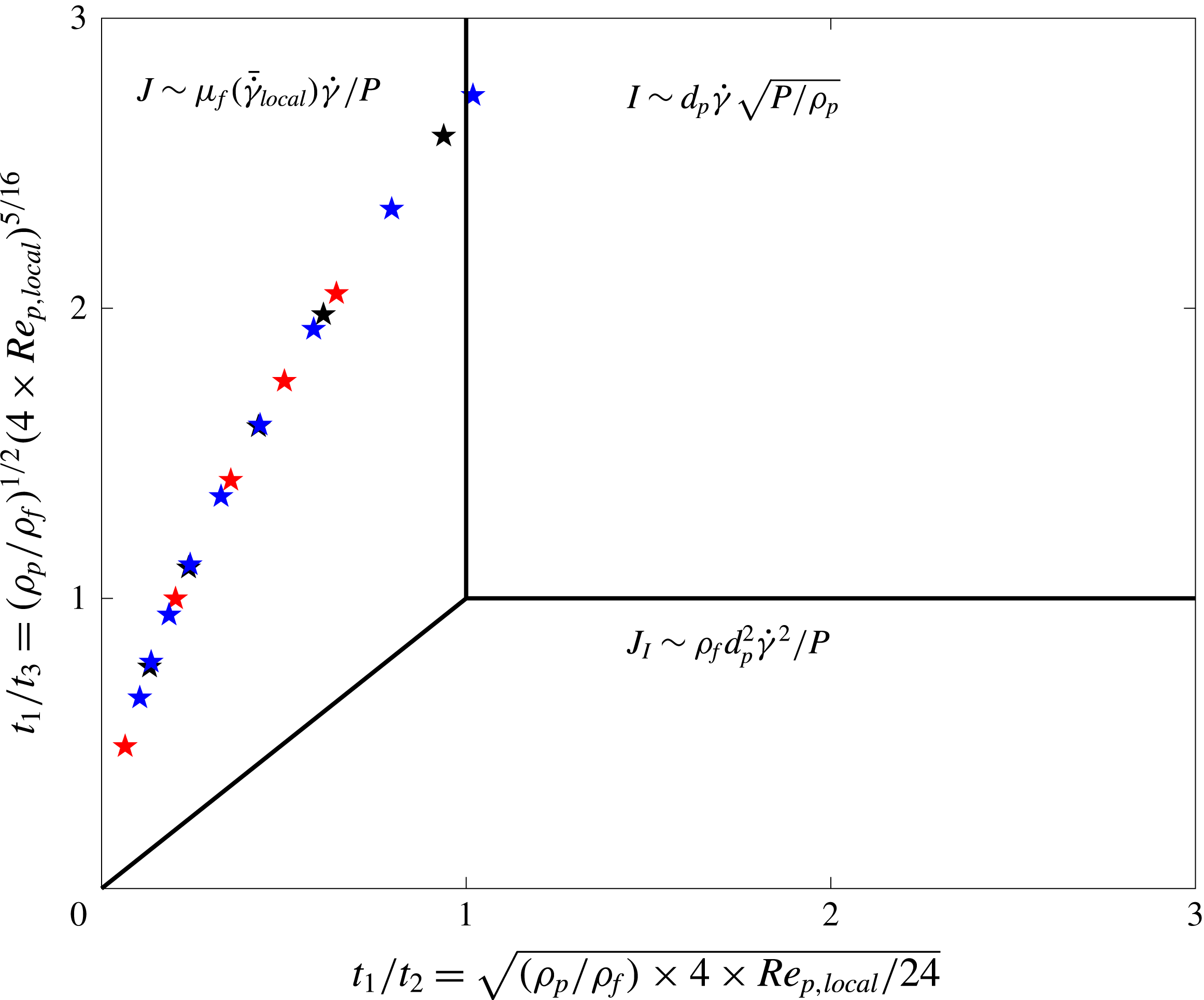
Figure 16. The phase diagram of three existing regimes for non-colloidal suspensions, styled after figure 7.13 in Andreotti et al. (Reference Andreotti, Forterre and Pouliquen2013).
To shed light on the role of inertia, we provide scalings for the different components of the stress. First, we show that the viscous stress
 $\unicode[STIX]{x1D70F}_{v}$
indeed scales viscously. To this end, we compute the ratio of the values of the viscous stresses in two successive simulations at constant solid volume fraction, cases
$\unicode[STIX]{x1D70F}_{v}$
indeed scales viscously. To this end, we compute the ratio of the values of the viscous stresses in two successive simulations at constant solid volume fraction, cases
 $(i)$
and
$(i)$
and
 $(i+1)$
, where we change the bulk shear rate from
$(i+1)$
, where we change the bulk shear rate from
 $\dot{\unicode[STIX]{x1D6FE}}(i)$
to
$\dot{\unicode[STIX]{x1D6FE}}(i)$
to
 $\dot{\unicode[STIX]{x1D6FE}}(i+1)$
. In the case of viscous scaling, we expect
$\dot{\unicode[STIX]{x1D6FE}}(i+1)$
. In the case of viscous scaling, we expect
 $\unicode[STIX]{x1D70F}_{v}(i+1)/\unicode[STIX]{x1D70F}_{v}(i)=[\dot{\unicode[STIX]{x1D6FE}}(i+1)/\dot{\unicode[STIX]{x1D6FE}}(i)]^{n}$
, where
$\unicode[STIX]{x1D70F}_{v}(i+1)/\unicode[STIX]{x1D70F}_{v}(i)=[\dot{\unicode[STIX]{x1D6FE}}(i+1)/\dot{\unicode[STIX]{x1D6FE}}(i)]^{n}$
, where
 $n=1$
for the Newtonian suspending fluid,
$n=1$
for the Newtonian suspending fluid,
 $n=0.3$
for the shear thinning suspending fluid and
$n=0.3$
for the shear thinning suspending fluid and
 $n=1.5$
for the shear thickening suspending fluid studied in this work. Figure 14(a–c) shows that our results follow the viscous scaling for all the cases. This also confirms the validity of our computational results.
$n=1.5$
for the shear thickening suspending fluid studied in this work. Figure 14(a–c) shows that our results follow the viscous scaling for all the cases. This also confirms the validity of our computational results.
Second, we investigate the scalings for the particle stress. Unlike the viscous stresses, the scale of particle stresses is not known a priori due to non-zero
 $Re_{p}$
in our simulations. We expect a scaling of the order of
$Re_{p}$
in our simulations. We expect a scaling of the order of
 $\unicode[STIX]{x1D70C}a^{2}\dot{\unicode[STIX]{x1D6FE}}^{2}$
when inertia is the main mechanism to transport momentum in a suspension. We therefore divide the values of the particle stresses in two successive simulations at constant solid volume fraction
$\unicode[STIX]{x1D70C}a^{2}\dot{\unicode[STIX]{x1D6FE}}^{2}$
when inertia is the main mechanism to transport momentum in a suspension. We therefore divide the values of the particle stresses in two successive simulations at constant solid volume fraction
 $(i)$
and
$(i)$
and
 $(i+1)$
, differing in the bulk shear rate
$(i+1)$
, differing in the bulk shear rate
 $\dot{\unicode[STIX]{x1D6FE}}(i)$
and
$\dot{\unicode[STIX]{x1D6FE}}(i)$
and
 $\dot{\unicode[STIX]{x1D6FE}}(i+1)$
. Figure 15(a–c) shows that for all types of suspending fluid
$\dot{\unicode[STIX]{x1D6FE}}(i+1)$
. Figure 15(a–c) shows that for all types of suspending fluid
 $\unicode[STIX]{x1D70F}_{p}(i+1)/\unicode[STIX]{x1D70F}_{p}(i)$
is slightly larger than
$\unicode[STIX]{x1D70F}_{p}(i+1)/\unicode[STIX]{x1D70F}_{p}(i)$
is slightly larger than
 $[\dot{\unicode[STIX]{x1D6FE}}(i+1)/\dot{\unicode[STIX]{x1D6FE}}(i)]^{n}$
indicating that the viscous scaling is still a reasonably good approximation and the inertial contribution to the transport of momentum is a secondary effect. To further confirm this, we report in figure 15(d)
$[\dot{\unicode[STIX]{x1D6FE}}(i+1)/\dot{\unicode[STIX]{x1D6FE}}(i)]^{n}$
indicating that the viscous scaling is still a reasonably good approximation and the inertial contribution to the transport of momentum is a secondary effect. To further confirm this, we report in figure 15(d)
 $\unicode[STIX]{x1D70F}_{p}(i+1)/\unicode[STIX]{x1D70F}_{p}(i)$
versus
$\unicode[STIX]{x1D70F}_{p}(i+1)/\unicode[STIX]{x1D70F}_{p}(i)$
versus
 $[\dot{\unicode[STIX]{x1D6FE}}(i+1)/\dot{\unicode[STIX]{x1D6FE}}(i)]^{2}$
; the data points all fall below an inertial scaling, although
$[\dot{\unicode[STIX]{x1D6FE}}(i+1)/\dot{\unicode[STIX]{x1D6FE}}(i)]^{2}$
; the data points all fall below an inertial scaling, although
 $Re_{p}$
is finite. From the analysis in the figure, the results in Picano et al. (Reference Picano, Breugem, Mitra and Brandt2013) and the stress budget reported above, we therefore conclude that inertial effects alter the suspension microstructure, in particular the particle relative motion, clearly breaking the fore–aft symmetry of Stokes flow, which induces shear thickening without altering the dominant viscous behaviour. Different to the case presented in Lashgari et al. (Reference Lashgari, Picano, Breugem and Brandt2014) where particles significantly alter the turbulent flow of a suspension, triggering a transition from a Reynolds stress inertial regime to a particle-dominated regime.
$Re_{p}$
is finite. From the analysis in the figure, the results in Picano et al. (Reference Picano, Breugem, Mitra and Brandt2013) and the stress budget reported above, we therefore conclude that inertial effects alter the suspension microstructure, in particular the particle relative motion, clearly breaking the fore–aft symmetry of Stokes flow, which induces shear thickening without altering the dominant viscous behaviour. Different to the case presented in Lashgari et al. (Reference Lashgari, Picano, Breugem and Brandt2014) where particles significantly alter the turbulent flow of a suspension, triggering a transition from a Reynolds stress inertial regime to a particle-dominated regime.
We therefore adopt a frictional view similar to that proposed in Cassar, Nicolas & Pouliquen (Reference Cassar, Nicolas and Pouliquen2005), Andreotti et al. (Reference Andreotti, Forterre and Pouliquen2013) to show that the main dimensionless number controlling the rheology of the suspensions studied here is associated with viscous stresses. Assuming an assembly of particles suspended in a viscous fluid that is subject to steady shear under a confining particle pressure
 $P$
, there exists only one dimensionless control parameter, i.e. the ratio of the microscopic time scale for the particle rearrangement to the macroscopic time scale of the flow
$P$
, there exists only one dimensionless control parameter, i.e. the ratio of the microscopic time scale for the particle rearrangement to the macroscopic time scale of the flow
 $\dot{\unicode[STIX]{x1D6FE}}^{-1}$
. The microscopic time scale can be determined by balancing the forces applied to a particle, i.e. the imposed pressure
$\dot{\unicode[STIX]{x1D6FE}}^{-1}$
. The microscopic time scale can be determined by balancing the forces applied to a particle, i.e. the imposed pressure
 $P$
and the drag force
$P$
and the drag force
 $F_{d}$
(Cassar et al.
Reference Cassar, Nicolas and Pouliquen2005; Andreotti et al.
Reference Andreotti, Forterre and Pouliquen2013). This implies the existence of the three following microscopic time scales
$F_{d}$
(Cassar et al.
Reference Cassar, Nicolas and Pouliquen2005; Andreotti et al.
Reference Andreotti, Forterre and Pouliquen2013). This implies the existence of the three following microscopic time scales
 $$\begin{eqnarray}t_{1}\sim \frac{d_{p}}{\sqrt{P/\unicode[STIX]{x1D70C}_{p}}},\quad t_{2}\sim \frac{d_{p}}{\sqrt{P/(\unicode[STIX]{x1D70C}_{f}Cd_{St})}},\quad t_{3}\sim \frac{d_{p}}{\sqrt{P/(\unicode[STIX]{x1D70C}_{f}Cd_{Turb})}},\quad \text{where }F_{d}=C_{d}d_{p}^{2}\unicode[STIX]{x1D70C}_{f}V^{2}.\end{eqnarray}$$
Here,
 $\unicode[STIX]{x1D70C}_{p}$
and
$\unicode[STIX]{x1D70C}_{p}$
and
 $d_{p}$
are the particle density and particle diameter, whereas the particle terminal velocity and its drag coefficient are denoted by
$d_{p}$
are the particle density and particle diameter, whereas the particle terminal velocity and its drag coefficient are denoted by
 $V$
and
$V$
and
 $C_{d}$
. When the drag force is negligible and the rearrangement of particles is solely governed by the imposed pressure, the relevant microscopic time scale is
$C_{d}$
. When the drag force is negligible and the rearrangement of particles is solely governed by the imposed pressure, the relevant microscopic time scale is
 $t_{1}$
, and consequently, the controlling dimensionless parameter
$t_{1}$
, and consequently, the controlling dimensionless parameter
 $I=t_{1}\dot{\unicode[STIX]{x1D6FE}}$
. When the imposed pressure balances the viscous drag force the microscopic time scale
$I=t_{1}\dot{\unicode[STIX]{x1D6FE}}$
. When the imposed pressure balances the viscous drag force the microscopic time scale
 $t_{2}=d_{p}/\sqrt{P/(\unicode[STIX]{x1D70C}_{f}Cd_{St})}$
, leading to the controlling dimensionless parameter
$t_{2}=d_{p}/\sqrt{P/(\unicode[STIX]{x1D70C}_{f}Cd_{St})}$
, leading to the controlling dimensionless parameter
 $J=t_{2}\dot{\unicode[STIX]{x1D6FE}}$
. Finally, the third scenario, when the imposed pressure balances the turbulent drag force on the particle, is associated with the microscopic time scale
$J=t_{2}\dot{\unicode[STIX]{x1D6FE}}$
. Finally, the third scenario, when the imposed pressure balances the turbulent drag force on the particle, is associated with the microscopic time scale
 $t_{3}$
and the controlling dimensionless parameter is
$t_{3}$
and the controlling dimensionless parameter is
 $J_{I}=t_{3}\dot{\unicode[STIX]{x1D6FE}}$
.
$J_{I}=t_{3}\dot{\unicode[STIX]{x1D6FE}}$
.
To calculate the values of the microscopic time scales
 $t_{2}$
and
$t_{2}$
and
 $t_{3}$
we need a closure for
$t_{3}$
we need a closure for
 $C_{d}$
. Following Hormozi & Frigaard (Reference Hormozi and Frigaard2017), we adopt the drag closure as follows
$C_{d}$
. Following Hormozi & Frigaard (Reference Hormozi and Frigaard2017), we adopt the drag closure as follows
 $$\begin{eqnarray}C_{d}(Re_{p,local})=\left\{\begin{array}{@{}ll@{}}\displaystyle \frac{24}{4\times Re_{p,local}}, & 4\times Re_{p,l}<1.4\\ \displaystyle \frac{24/1.4^{0.375}}{(4\times Re_{p,local})^{0.625}}, & 1.4\leqslant 4\times Re_{p,l}\leqslant 500.\end{array}\right.\end{eqnarray}$$
Note that the multiplier
 $4$
appears in front of
$4$
appears in front of
 $Re_{p,local}$
since our local particle Reynolds number is based on the particle radius, not the particle diameter. The above closure for the drag coefficient allows us to calculate the ratio of the microscopic time scales:
$Re_{p,local}$
since our local particle Reynolds number is based on the particle radius, not the particle diameter. The above closure for the drag coefficient allows us to calculate the ratio of the microscopic time scales:
 $t_{1}/t_{2}=\sqrt{(\unicode[STIX]{x1D70C}_{p}/\unicode[STIX]{x1D70C}_{f})\times 4\times Re_{p,local}/24}$
and
$t_{1}/t_{2}=\sqrt{(\unicode[STIX]{x1D70C}_{p}/\unicode[STIX]{x1D70C}_{f})\times 4\times Re_{p,local}/24}$
and
 $t_{1}/t_{3}=(\unicode[STIX]{x1D70C}_{p}/\unicode[STIX]{x1D70C}_{f})^{1/2}(4\times Re_{p,local})^{5/16}$
. Figure 16 shows the phase diagram for the three regimes of non-colloidal suspensions in the plane
$t_{1}/t_{3}=(\unicode[STIX]{x1D70C}_{p}/\unicode[STIX]{x1D70C}_{f})^{1/2}(4\times Re_{p,local})^{5/16}$
. Figure 16 shows the phase diagram for the three regimes of non-colloidal suspensions in the plane
 $(t_{1}/t_{2},t_{1}/t_{3})$
. This map is styled after figure 7.13 in Andreotti et al. (Reference Andreotti, Forterre and Pouliquen2013) (see Hormozi & Frigaard Reference Hormozi and Frigaard2017, for a detailed explanation).
$(t_{1}/t_{2},t_{1}/t_{3})$
. This map is styled after figure 7.13 in Andreotti et al. (Reference Andreotti, Forterre and Pouliquen2013) (see Hormozi & Frigaard Reference Hormozi and Frigaard2017, for a detailed explanation).
Three regimes can be identified in the frictional map shown in figure 16. The first regime is associated with suspensions in which
 $t_{1}\gtrsim t_{2}$
and
$t_{1}\gtrsim t_{2}$
and
 $t_{1}\gtrsim t_{3}$
, where the dominant microscopic time scale is
$t_{1}\gtrsim t_{3}$
, where the dominant microscopic time scale is
 $t_{1}$
and the primary controlling dimensionless number is
$t_{1}$
and the primary controlling dimensionless number is
 $I\sim d_{p}\dot{\unicode[STIX]{x1D6FE}}\sqrt{P/\unicode[STIX]{x1D70C}_{p}}$
. In this regime the main mechanism responsible for the momentum transport is that associated with particle contacts and collisions, i.e. in this regime particle inertia dominates. The second regime, when
$I\sim d_{p}\dot{\unicode[STIX]{x1D6FE}}\sqrt{P/\unicode[STIX]{x1D70C}_{p}}$
. In this regime the main mechanism responsible for the momentum transport is that associated with particle contacts and collisions, i.e. in this regime particle inertia dominates. The second regime, when
 $t_{2}\gtrsim t_{1}$
and
$t_{2}\gtrsim t_{1}$
and
 $t_{2}\gtrsim t_{3}$
, has
$t_{2}\gtrsim t_{3}$
, has
 $t_{2}$
as the dominant microscopic time scale and
$t_{2}$
as the dominant microscopic time scale and
 $J\sim \unicode[STIX]{x1D707}_{f}(\bar{\dot{\unicode[STIX]{x1D6FE}}}_{local})\dot{\unicode[STIX]{x1D6FE}}/P$
as the primary controlling dimensionless number. In this regime, the viscous stresses are the main mechanism for momentum transport, the viscous drag regime. The third regime, when
$J\sim \unicode[STIX]{x1D707}_{f}(\bar{\dot{\unicode[STIX]{x1D6FE}}}_{local})\dot{\unicode[STIX]{x1D6FE}}/P$
as the primary controlling dimensionless number. In this regime, the viscous stresses are the main mechanism for momentum transport, the viscous drag regime. The third regime, when
 $t_{3}$
is the dominant microscopic time scale, with relevant the dimensionless number
$t_{3}$
is the dominant microscopic time scale, with relevant the dimensionless number
 $J_{I}\sim \unicode[STIX]{x1D70C}_{f}d_{p}^{2}\dot{\unicode[STIX]{x1D6FE}}^{2}/P$
, is dominated by the Reynolds stresses of the fluid phase, i.e. the turbulent drag at the particle scale (inertial drag regime).
$J_{I}\sim \unicode[STIX]{x1D70C}_{f}d_{p}^{2}\dot{\unicode[STIX]{x1D6FE}}^{2}/P$
, is dominated by the Reynolds stresses of the fluid phase, i.e. the turbulent drag at the particle scale (inertial drag regime).
Note that this frictional framework is relevant for dense suspensions in which the particle phase pressure is significant. Moreover, the boundaries between the three regimes discussed above and shown in figure 16 are unknown a priori and finding the exact locations would require an extensive experimental or computational study. Here, we wish to determine the regime that our simulations for suspensions with
 $\unicode[STIX]{x1D6F7}=0.4$
belong to. It is reasonable to assume that a
$\unicode[STIX]{x1D6F7}=0.4$
belong to. It is reasonable to assume that a
 $40\,\%$
solid volume fraction is dense enough that the particle phase pressure
$40\,\%$
solid volume fraction is dense enough that the particle phase pressure
 $P$
is significant, and consequently, the frictional view just introduced can be used to characterise the suspension regimes. Figure 16 shows that all of the dense simulations considered here (i.e.
$P$
is significant, and consequently, the frictional view just introduced can be used to characterise the suspension regimes. Figure 16 shows that all of the dense simulations considered here (i.e.
 $\unicode[STIX]{x1D6F7}=0.4$
) fall into the regime where the viscous stresses play the main roles in the momentum transport, and hence, the viscous number
$\unicode[STIX]{x1D6F7}=0.4$
) fall into the regime where the viscous stresses play the main roles in the momentum transport, and hence, the viscous number
 $J$
is the controlling dimensionless parameter. Therefore, viscous forces are mainly responsible for the dissipation of the power or energy given to the bulk of these suspensions, although
$J$
is the controlling dimensionless parameter. Therefore, viscous forces are mainly responsible for the dissipation of the power or energy given to the bulk of these suspensions, although
 $Re_{p}$
is non-zero.
$Re_{p}$
is non-zero.
The above discussion raises the question of the role of inertia for the suspensions under investigation here and its influence on the effective viscosity. As shown in § 3.4, increasing
 $Re_{p}$
results in an enhancement of the suspension effective viscosity. This is attributed to excluded volume effects in the work by Picano et al. (Reference Picano, Breugem, Mitra and Brandt2013): the effective volume fraction of the suspension is higher than the nominal one because of the ‘shadow’ region (a region with statistically vanishing relative particle flux) around the particles due to inertia in the relative particle motion. Therefore, finite inertia affects the suspension microstructure by increasing the effective
$Re_{p}$
results in an enhancement of the suspension effective viscosity. This is attributed to excluded volume effects in the work by Picano et al. (Reference Picano, Breugem, Mitra and Brandt2013): the effective volume fraction of the suspension is higher than the nominal one because of the ‘shadow’ region (a region with statistically vanishing relative particle flux) around the particles due to inertia in the relative particle motion. Therefore, finite inertia affects the suspension microstructure by increasing the effective
 $\unicode[STIX]{x1D6F7}$
, which, in turn, enhances the viscous dissipation. This is why the enhancement of the effective viscosity with inertia is secondary with respect to increases of the nominal solid volume fraction and the suspension viscosity can be scaled back to the Eilers fit, obtained for Stokesian suspensions (see Picano et al.
Reference Picano, Breugem, Mitra and Brandt2013).
$\unicode[STIX]{x1D6F7}$
, which, in turn, enhances the viscous dissipation. This is why the enhancement of the effective viscosity with inertia is secondary with respect to increases of the nominal solid volume fraction and the suspension viscosity can be scaled back to the Eilers fit, obtained for Stokesian suspensions (see Picano et al.
Reference Picano, Breugem, Mitra and Brandt2013).
Our study shows that the boundary between the inertial
 $I$
-dominated and the viscous
$I$
-dominated and the viscous
 $J$
-dominated regimes, as estimated by scaling arguments with no prefactor, is a good approximation to the real one at least for the suspensions examined here, see figure 16. Despite non-zero values of
$J$
-dominated regimes, as estimated by scaling arguments with no prefactor, is a good approximation to the real one at least for the suspensions examined here, see figure 16. Despite non-zero values of
 $Re_{p}$
in our simulations, we are not in the regime where the particle inertia dominates, and therefore, closures for the suspension stresses should differ from those given in the recent studies by Trulsson et al. (Reference Trulsson, Andreotti and Claudin2012). In fact the inertia affects the microstructure and can be included in the suspension stress closure as follows
$Re_{p}$
in our simulations, we are not in the regime where the particle inertia dominates, and therefore, closures for the suspension stresses should differ from those given in the recent studies by Trulsson et al. (Reference Trulsson, Andreotti and Claudin2012). In fact the inertia affects the microstructure and can be included in the suspension stress closure as follows
 $$\begin{eqnarray}\displaystyle & \displaystyle \unicode[STIX]{x1D70F}=G(\unicode[STIX]{x1D6F7}+\unicode[STIX]{x1D6FF}\unicode[STIX]{x1D6F7}(\unicode[STIX]{x1D6F7},Re_{p,local}))\unicode[STIX]{x1D707}_{0}\hat{\unicode[STIX]{x1D707}}(\bar{\dot{\unicode[STIX]{x1D6FE}}}_{local}(\unicode[STIX]{x1D6F7}))\dot{\unicode[STIX]{x1D6FE}}, & \displaystyle\end{eqnarray}$$
 $$\begin{eqnarray}\displaystyle & \displaystyle \unicode[STIX]{x1D6FF}\unicode[STIX]{x1D6F7}=0.9\times Re_{p,local}\unicode[STIX]{x1D6F7}^{2}(1-\unicode[STIX]{x1D6F7}/\unicode[STIX]{x1D6F7}_{max})^{3}. & \displaystyle\end{eqnarray}$$
Here,
 $\unicode[STIX]{x1D6FF}\unicode[STIX]{x1D6F7}$
is the increase in the nominal volume fraction due to the excluded volume effects mentioned above. Equation (3.16) provides an estimation of this increase of effective volume fraction by fitting the simulation results of Picano et al. (Reference Picano, Breugem, Mitra and Brandt2013) in which
$\unicode[STIX]{x1D6FF}\unicode[STIX]{x1D6F7}$
is the increase in the nominal volume fraction due to the excluded volume effects mentioned above. Equation (3.16) provides an estimation of this increase of effective volume fraction by fitting the simulation results of Picano et al. (Reference Picano, Breugem, Mitra and Brandt2013) in which
 $\unicode[STIX]{x1D6FF}\unicode[STIX]{x1D6F7}$
is obtained by computing the volume of the so-called ‘shadow’ regions. Note that the form of (3.16) is chosen to satisfy the following conditions. First, at small
$\unicode[STIX]{x1D6FF}\unicode[STIX]{x1D6F7}$
is obtained by computing the volume of the so-called ‘shadow’ regions. Note that the form of (3.16) is chosen to satisfy the following conditions. First, at small
 $\unicode[STIX]{x1D6F7}$
, we expect
$\unicode[STIX]{x1D6F7}$
, we expect
 $\unicode[STIX]{x1D6FF}\unicode[STIX]{x1D6F7}$
to be proportional to
$\unicode[STIX]{x1D6FF}\unicode[STIX]{x1D6F7}$
to be proportional to
 $\unicode[STIX]{x1D6F7}^{2}$
, since at least two-particle interactions are needed to give rise to the excluded volume effect. Second, the excluded volume must vanish as
$\unicode[STIX]{x1D6F7}^{2}$
, since at least two-particle interactions are needed to give rise to the excluded volume effect. Second, the excluded volume must vanish as
 $\unicode[STIX]{x1D6F7}\rightarrow \unicode[STIX]{x1D6F7}_{max}$
. In summary, the closure (3.15) provides the suspension shear stress for Newtonian and generalised Newtonian suspending fluids where the microstructure modifications induced by inertia are coded into the
$\unicode[STIX]{x1D6F7}\rightarrow \unicode[STIX]{x1D6F7}_{max}$
. In summary, the closure (3.15) provides the suspension shear stress for Newtonian and generalised Newtonian suspending fluids where the microstructure modifications induced by inertia are coded into the
 $G$
function. We note again here that this closure is valid for suspension in which viscous effects are the still main mechanism for momentum transport, while inertial effects are mainly responsible for changing the microstructure. Note that the local Reynolds number seen by the particles,
$G$
function. We note again here that this closure is valid for suspension in which viscous effects are the still main mechanism for momentum transport, while inertial effects are mainly responsible for changing the microstructure. Note that the local Reynolds number seen by the particles,
 $Re_{p,local}$
, is the appropriate dimensionless number to model the effects of the microstructure.
$Re_{p,local}$
, is the appropriate dimensionless number to model the effects of the microstructure.
4 Conclusion and remarks
We study suspensions of neutrally buoyant spheres in both Newtonian and inelastic non-Newtonian fluids, using interface-resolved direct numerical simulations. The Carreau and power-law models are employed to describe the rheological behaviour of shear thinning and shear thickening carrier fluids, where the fluid viscosity varies instantaneously with the local flow shear rate,
 $\dot{\unicode[STIX]{x1D6FE}}_{local}(x,y,z)$
. The simulations are performed in a plane Couette configuration. The rheological parameters of the suspending fluids and the particle phase properties are kept constant while we change the volume fraction of the solid phase,
$\dot{\unicode[STIX]{x1D6FE}}_{local}(x,y,z)$
. The simulations are performed in a plane Couette configuration. The rheological parameters of the suspending fluids and the particle phase properties are kept constant while we change the volume fraction of the solid phase,
 $0\leqslant \unicode[STIX]{x1D6F7}\leqslant 40\,\%$
, and the applied shear rate. This allows us to study inertial suspensions with
$0\leqslant \unicode[STIX]{x1D6F7}\leqslant 40\,\%$
, and the applied shear rate. This allows us to study inertial suspensions with
 $0<Re_{p}\leqslant 10$
. We focus on the bulk properties of the suspension as well as the local behaviour of the particles and the carrier fluid. The main findings of our work are summarised as follows.
$0<Re_{p}\leqslant 10$
. We focus on the bulk properties of the suspension as well as the local behaviour of the particles and the carrier fluid. The main findings of our work are summarised as follows.
The local profile of solid volume fractions show particle layering for nominal volume fractions
 $\unicode[STIX]{x1D6F7}\geqslant 30\,\%$
, with the peak of the layers located close to the wall. The distribution of particles across the Couette cell is mainly controlled by geometry and confinement effects, with a weaker dependency on the type of suspending fluid and inertial effects. However, the latter has a strong influence on the velocity profiles of the particle and fluid phases. In the cases with non-Newtonian suspending fluids, viscosity at the particle scale depends on the local shear rate. This results in a larger and smaller local particle Reynolds number as the shear thinning and thickening degree increase, respectively. Inertia also induces a slip velocity between solid and fluid phases with a maximum value close to the wall and zero at the gap centre. This suggests that a suspension flow should be formulated with a two-phase continuum framework close to the walls, where inertial effects are first apparent, although a mixture continuum framework can still provide reasonable predictions of the flow away from the walls, i.e. around the central region. Note that this is also observed for turbulent suspensions and has been successfully used in Costa et al. (Reference Costa, Picano, Brandt and Breugem2016) to predict turbulent drag in channel flows.
$\unicode[STIX]{x1D6F7}\geqslant 30\,\%$
, with the peak of the layers located close to the wall. The distribution of particles across the Couette cell is mainly controlled by geometry and confinement effects, with a weaker dependency on the type of suspending fluid and inertial effects. However, the latter has a strong influence on the velocity profiles of the particle and fluid phases. In the cases with non-Newtonian suspending fluids, viscosity at the particle scale depends on the local shear rate. This results in a larger and smaller local particle Reynolds number as the shear thinning and thickening degree increase, respectively. Inertia also induces a slip velocity between solid and fluid phases with a maximum value close to the wall and zero at the gap centre. This suggests that a suspension flow should be formulated with a two-phase continuum framework close to the walls, where inertial effects are first apparent, although a mixture continuum framework can still provide reasonable predictions of the flow away from the walls, i.e. around the central region. Note that this is also observed for turbulent suspensions and has been successfully used in Costa et al. (Reference Costa, Picano, Brandt and Breugem2016) to predict turbulent drag in channel flows.
We present the probability density function of the local shear rate, revealing the existence of a wide spectrum of local shear rates; this depends primarily on
 $\unicode[STIX]{x1D6F7}$
and secondarily on
$\unicode[STIX]{x1D6F7}$
and secondarily on
 $Re_{p}$
, which implies the deficiency of theoretical approaches based on mean field values in explaining the mechanics of suspensions. Mean field theories (e.g. Chateau et al.
Reference Chateau, Ovarlez and Trung2008) should be refined to include higher moments, including possibly minima and maxima, of the local shear rate distribution. This requires further investigation and improvement of the available model frameworks.
$Re_{p}$
, which implies the deficiency of theoretical approaches based on mean field values in explaining the mechanics of suspensions. Mean field theories (e.g. Chateau et al.
Reference Chateau, Ovarlez and Trung2008) should be refined to include higher moments, including possibly minima and maxima, of the local shear rate distribution. This requires further investigation and improvement of the available model frameworks.
We demonstrate that the non-dimensional relative viscosity of the suspensions with non-Newtonian carrier fluids can be well predicted by the homogenisation theory of Chateau et al. (Reference Chateau, Ovarlez and Trung2008) in the limit of
 $Re_{p}\rightarrow 0$
, and more accurately for lower
$Re_{p}\rightarrow 0$
, and more accurately for lower
 $\unicode[STIX]{x1D6F7}$
. However, adding inertia to the system alters the microstructure and results in a deviation of the relative viscosity of the suspensions from the Stokesian prediction, while the main dissipation mechanism is still viscous. In fact, we show that for the parameter range explored here both particle stresses and fluid stresses are clustered about viscous scalings. We therefore adopt the frictional view of Cassar et al. (Reference Cassar, Nicolas and Pouliquen2005), Andreotti et al. (Reference Andreotti, Forterre and Pouliquen2013) to show that the main dimensionless number controlling the mechanics of suspensions is the so-called viscous number,
$\unicode[STIX]{x1D6F7}$
. However, adding inertia to the system alters the microstructure and results in a deviation of the relative viscosity of the suspensions from the Stokesian prediction, while the main dissipation mechanism is still viscous. In fact, we show that for the parameter range explored here both particle stresses and fluid stresses are clustered about viscous scalings. We therefore adopt the frictional view of Cassar et al. (Reference Cassar, Nicolas and Pouliquen2005), Andreotti et al. (Reference Andreotti, Forterre and Pouliquen2013) to show that the main dimensionless number controlling the mechanics of suspensions is the so-called viscous number,
 $J\sim \unicode[STIX]{x1D707}_{f}(\bar{\dot{\unicode[STIX]{x1D6FE}}}_{local})\dot{\unicode[STIX]{x1D6FE}}/P$
, confirming that viscous stresses are responsible for the momentum transport even when the particle Reynolds number is finite. However, due to inertial effects, the microstructure becomes anisotropic and so-called shadow regions form around particles (these are regions with zero probability of finding another particle, see Picano et al.
Reference Picano, Breugem, Mitra and Brandt2013). This enhances the effective particle volume fraction, and consequently, the viscous dissipation and relative viscosity. We have estimated the volume of these shadow regions from our simulations and included this microstructural effect into a functional form for the relative viscosity. In this way, we provide a prediction for the added excluded volume due to inertia and a closure for the suspension stress in the case of both Newtonian and generalised Newtonian suspending fluids valid for
$J\sim \unicode[STIX]{x1D707}_{f}(\bar{\dot{\unicode[STIX]{x1D6FE}}}_{local})\dot{\unicode[STIX]{x1D6FE}}/P$
, confirming that viscous stresses are responsible for the momentum transport even when the particle Reynolds number is finite. However, due to inertial effects, the microstructure becomes anisotropic and so-called shadow regions form around particles (these are regions with zero probability of finding another particle, see Picano et al.
Reference Picano, Breugem, Mitra and Brandt2013). This enhances the effective particle volume fraction, and consequently, the viscous dissipation and relative viscosity. We have estimated the volume of these shadow regions from our simulations and included this microstructural effect into a functional form for the relative viscosity. In this way, we provide a prediction for the added excluded volume due to inertia and a closure for the suspension stress in the case of both Newtonian and generalised Newtonian suspending fluids valid for
 $O(Re_{p})\sim 10$
. Note also that once the effective volume fraction is considered, Eilers fit is able to predict the suspension viscosity, confirming that we are still in the viscous regime.
$O(Re_{p})\sim 10$
. Note also that once the effective volume fraction is considered, Eilers fit is able to predict the suspension viscosity, confirming that we are still in the viscous regime.
Concerning the frictional framework of Cassar et al. (Reference Cassar, Nicolas and Pouliquen2005) and Andreotti et al. (Reference Andreotti, Forterre and Pouliquen2013), we note that this view provides scaling for the suspension stresses but no information about the microstructural effects. Therefore, refinements of existing rheological laws would need to include microstructural effects; these local details of the suspension flow can be obtained by well-resolved experimental or computational data, as done here. Our study shows that the so-called inertial shear thickening mode introduced by Picano et al. (Reference Picano, Breugem, Mitra and Brandt2013) belongs to the viscous class of suspensions, yet the inertial microstructure needs to be taken into account to accurately predict the suspension rheology.
This study raises a series of research questions requiring further investigation. First, we show that as we change the type of suspending fluid the contribution of particle stress to the total suspension stress changes. In our system, this is most likely mainly due to the change in the stresslet. A systematic study may therefore be devoted to the investigation of the dependency of the stresslet on the non-Newtonian behaviour of the suspending fluid and its influence on the bulk rheology. Second, the simulations presented here fall into the viscous-dominated suspension regime, although we show how microstructural effects due to inertia are not at all negligible. One may therefore further explore the frictional map by performing simulations/experiments for a wider range of
 $\unicode[STIX]{x1D6F7}$
and
$\unicode[STIX]{x1D6F7}$
and
 $Re_{p}$
, one goal being to determine the boundaries between the viscous- and inertia-dominated transport mechanisms. Such an analysis would also suggest how to include microstructural effects in order to refine rheological laws. Third, we consider here the simplest shear flow, with homogeneous bulk shear rate. It is not obvious how inhomogeneous bulk shear rates change the results and how non-local rheology comes into play (see e.g. Pouliquen & Forterre Reference Pouliquen and Forterre2009; Bouzid et al.
Reference Bouzid, Trulsson, Claudin, Clément and Andreotti2013; Henann & Kamrin Reference Henann and Kamrin2014; Kamrin & Henann Reference Kamrin and Henann2015). Finally, theoretical approaches based on mean field theory should be improved to include the consequences of the wide spectrum of the local shear rate. To this end, it is essential to study complex features of suspensions with non-Newtonian suspending fluids.
$Re_{p}$
, one goal being to determine the boundaries between the viscous- and inertia-dominated transport mechanisms. Such an analysis would also suggest how to include microstructural effects in order to refine rheological laws. Third, we consider here the simplest shear flow, with homogeneous bulk shear rate. It is not obvious how inhomogeneous bulk shear rates change the results and how non-local rheology comes into play (see e.g. Pouliquen & Forterre Reference Pouliquen and Forterre2009; Bouzid et al.
Reference Bouzid, Trulsson, Claudin, Clément and Andreotti2013; Henann & Kamrin Reference Henann and Kamrin2014; Kamrin & Henann Reference Kamrin and Henann2015). Finally, theoretical approaches based on mean field theory should be improved to include the consequences of the wide spectrum of the local shear rate. To this end, it is essential to study complex features of suspensions with non-Newtonian suspending fluids.
Acknowledgements
Parts of this research were supported by NSF (grant no. CBET-1554044-CAREER) and NSF-ERC (grant no. CBET-1641152 Supplementary CAREER) via the research awards (S.H.). L.B. acknowledges financial support by the European Research Council Grant no. ERC-2013-CoG- 616186, TRITOS. The authors acknowledge computer time provided by SNIC (Swedish National Infrastructure for Computing).


