2.1. Turbulence closure model

While computational power has improved immensely in recent decades, for many fluid mechanics problems, it is still not practically feasible to resolve the small scales required for either DNS or LES. Rather, it is often necessary in practice to work with a Reynolds-averaged description of the flow, with the effects of turbulence on the mean flow accounted for with the aid of a turbulence closure model. For this purpose, the present study focuses on the Wilcox (Reference Wilcox2006) stress–$\omega$ model (where $\omega$ is again the specific dissipation rate of turbulence). This model, in a form suitable for a two-phase (water–air) fluid mixture, consists of the following stress-transport equations:

(2.1)\begin{align} \underbrace{\frac{ \partial \bar{\rho} \tau_{ij}}{\partial t} }_{\text{Time variation}} + \underbrace{ \bar{u}_k \frac{\partial \bar{\rho} \tau_{ij}}{\partial x_k}}_{\text{Convection}} &={-}\underbrace{\bar{\rho} P_{ij}}_{\text{Production}} +\underbrace{ \frac{2}{3} \bar{\rho} \beta^* \omega k \delta_{ij}}_{\text{Dissipation}} -\underbrace{\bar{\rho} \varPi_{ij} }_{\text{Pressure-strain}}\nonumber\\ &\quad + \underbrace{\bar{\rho} \alpha_b^* \frac{k}{\omega} N_{ij}}_{\text{Buoyancy production}} +\underbrace{ \frac{\partial}{\partial x_k}\left[\bar{\rho} (\nu + \sigma^*\frac{k}{\omega})\frac{\partial \tau_{ij}}{\partial x_k} \right] }_{\text{Diffusion}} \end{align}

combined with a separate transport equation for the specific rate of dissipation $\omega$:

(2.2)\begin{align} \underbrace{ \frac{\partial \bar{\rho}\omega}{\partial t} }_{\text{Time variation}} + \underbrace{ \bar{u}_j \frac{\partial \bar{\rho} \omega}{\partial x_j}}_{\text{Convection}} &= \underbrace{ \bar{\rho} \alpha \frac{\omega}{k} \tau_{ij}\frac{\partial \bar{u}_i}{\partial x_j}}_{\text{Production}} - \underbrace{\bar{\rho} \beta \omega^2 }_{\text{Dissipation}} + \underbrace{\sigma_d \frac{\bar{\rho}}{\omega} \frac{\partial k}{\partial x_j}\frac{\partial \omega}{\partial x_j} }_{\text{Cross-diffusion}} \nonumber\\ &\quad + \underbrace{ \frac{\partial}{\partial x_k} \left[ \bar{\rho}\left(\nu + \sigma \frac{k}{\omega}\right)\frac{\partial \omega}{\partial x_k}\right] } _{\text{Diffusion}}. \end{align}

In the above, $x_j$ are the Cartesian coordinates, $\bar {u}_j$ are the mean (Reynolds-averaged) components of the velocity, $g_j$ is gravitational acceleration, $\delta _{ij}$ is the Kronecker delta, $\nu$ is the kinematic fluid viscosity, $\bar {\rho }$ is the fluid density and $t$ is time. The specific Reynolds stress tensor is defined as

(2.3)\begin{equation} \tau_{ij} ={-} \overline{u_{i}^\prime u_{j}^\prime}, \end{equation}

where a prime denotes turbulent fluctuations and the overbar denotes Reynolds averaging. The turbulent kinetic energy (per unit mass) is thus

(2.4)\begin{equation} k ={-} \tfrac{1}{2} \tau_{kk}. \end{equation}

Buoyancy production (as derived in Appendix A) is included with terms proportional to the Brunt–Väisälä frequency tensor:

(2.5)\begin{equation} N_{ij}= \frac{1}{\rho_0} \left( g_i\frac{\partial \bar{\rho}}{\partial x_j} + g_j\frac{\partial \bar{\rho}}{\partial x_i}\right), \end{equation}

where $\rho _0$ is the constant reference density of the fluid.

The pressure–strain correlation is

(2.6)\begin{align} \varPi_{ij}&=\beta^* C_1 \omega\left(\tau_{ij}+\tfrac{2}{3}k\delta_{ij}\right) -\hat{\alpha}(P_{ij}-\tfrac{2}{3}P\delta_{ij}) \nonumber\\ &\quad -\hat{\beta}\left(D_{ij}-\tfrac{2}{3}P\delta_{ij}\right) -\hat{\gamma}k\left(S_{ij}-\tfrac{1}{3}S_{kk}\delta_{ij}\right), \end{align}

where

(2.7)$$\begin{gather} P_{ij}=\tau_{im}\frac{\partial \bar{u}_j}{\partial x_m}+\tau_{jm} \frac{\partial \bar{u}_i}{\partial x_m}, \end{gather}$$

(2.8)$$\begin{gather}D_{ij}=\tau_{im}\frac{\partial \bar{u}_m}{\partial x_j}+\tau_{jm}\frac{\partial \bar{u}_m}{\partial x_i}, \end{gather}$$

(2.9)$$\begin{gather}S_{ij}= \frac{1}{2} \left( \frac{\partial \bar{u}_i}{\partial x_j} + \frac{\partial \bar{u}_j}{\partial x_i} \right), \end{gather}$$

(2.10)$$\begin{gather}P=\tfrac{1}{2}P_{kk}. \end{gather}$$

The model closure coefficients, taken directly from Wilcox (Reference Wilcox2006), are defined as follows:

(2.11)\begin{gather} \left.\begin{array}{cccc@{}} C_1=1.8, & C_2=10/19, & \hat{\alpha}=(8+C_2)/11, & \hat{\beta}=(8C_2-2)/11, \\ \hat{\gamma}=(60C_2-4)/55, & \alpha=0.52, & \beta^*=0.09, & \beta_0=0.0708, \\ \beta=\beta_0 f_{\beta}, & \sigma=0.5, & \sigma^*=0.6, & \sigma_{d0}=0.125, \end{array}\right\} \end{gather}

(2.12)\begin{gather} \sigma_d=\begin{cases} 0, & \displaystyle \frac{\partial k}{\partial x_j}\frac{\partial \omega}{\partial x_j} \leqslant 0 \\ \sigma_{d0}, & \displaystyle \frac{\partial k}{\partial x_j}\frac{\partial \omega}{\partial x_j} > 0, \end{cases} \end{gather}

(2.13a–c)\begin{gather} f_{\beta}=\frac{1+85 \chi_{\omega}}{1+100 \chi_{\omega}},\quad \chi_{\omega}=\left\vert\frac{\varOmega_{ij}\varOmega_{jk}\hat{S}_{ki}}{(\beta^* \omega)^3} \right\vert, \quad \hat{S}_{ki}=S_{ki}-\frac{1}{2}\frac{\partial \bar{u}_m}{\partial x_m} \delta_{ki}, \end{gather}

with $\alpha _b^*=1.36$ (following Larsen & Fuhrman (Reference Larsen and Fuhrman2018); see also Appendix A). Unless explicitly stated otherwise, this value is fixed in what follows. A detailed description of the closure evolution from third-order turbulence correlations to second-order ones can be found in Wilcox (Reference Wilcox2006, pp. 41–43) and Launder et al. (Reference Launder, Reece and Rodi1975, their § 3).

Compared with the LRR (Launder et al. Reference Launder, Reece and Rodi1975) stress–$\varepsilon$ model, the $\omega$-based stress-transport model formulated above reduces the complexity of the diffusion term and the pressure–strain relation considerably. Moreover, since the $\omega$ equation yields better near-wall behaviour, the pressure–strain relation does not require an artificial wall-reflection term. (As discussed by Parneix, Laurence & Durbin (Reference Parneix, Laurence and Durbin1998), the LRR wall-reflection term is more to mitigate a deficiency in the $\varepsilon$ equation than to correctly or physically represent the pressure-echo process.) We therefore adopt the Wilcox (Reference Wilcox2006) stress–$\omega$ model as our primary focus for both analysis and applications in what follows.

2.2. Stability analysis

As shown and explained by Mayer & Madsen (Reference Mayer and Madsen2000), Larsen & Fuhrman (Reference Larsen and Fuhrman2018) and Fuhrman & Li (Reference Fuhrman and Li2020) (see also § 7.6 of Sumer & Fuhrman (Reference Sumer and Fuhrman2020)), standard two-equation turbulence closure models can result in turbulence over-production in the potential flow core region beneath surface waves. This is due to their inherent instability in such regions, leading to non-physical exponential growth of the turbulent kinetic energy and eddy viscosity. Computational results of Brown et al. (Reference Brown, Greaves, Magar and Conley2016), who used the LRR stress–$\varepsilon$ turbulence model to simulate breaking waves, demonstrated seemingly similar turbulence over-production prior to incipient wave breaking. This suggests that RSMs may share the same inherent instability in nearly potential flow regions having finite strain. It is therefore of interest to extend the analysis of Larsen & Fuhrman (Reference Larsen and Fuhrman2018) to consider the formal asymptotic stability of RSMs. In what follows in the main text we formally analyse the Wilcox (Reference Wilcox2006) stress–$\omega$ model. Similar analysis (and findings) of the LRR stress–$\varepsilon$ model is provided in Appendix B for completeness.

Consider now an incompressible fluid region having constant density beneath a small-amplitude plane surface wave train propagating in the horizontal $x_1=x$ direction, where the turbulence model described above is active. We will assume the mean flow is described by linear potential flow (Stokes first-order) wave theory, with velocity fields

(2.14)$$\begin{gather} \bar{u}_1=u=\frac{H \sigma_{w}}{2} \frac{\cosh (k_w y)}{\sinh (k_w h)} \cos(k_w x - \sigma_{w} t), \end{gather}$$

(2.15)$$\begin{gather}\bar{u}_2=v=\frac{H \sigma_{w}}{2} \frac{\sinh (k_w y)}{\sinh (k_w h)} \sin(k_w x - \sigma_{w} t), \end{gather}$$

where the vertical $x_2=y$ axis is placed at the bed, $\sigma _{w}$ is the angular wave frequency, $k_w$ is the wavenumber, $h$ is the water depth and $H$ is the wave height.

Following Mayer & Madsen (Reference Mayer and Madsen2000), Larsen & Fuhrman (Reference Larsen and Fuhrman2018) and Fuhrman & Li (Reference Fuhrman and Li2020), diffusive and convective terms are neglected in the analysis, which is reasonable in the potential flow region. Meanwhile, the buoyancy production term goes to zero in the region beneath surface waves where the density is again assumed constant. From the assumptions stated above, (2.1) and (2.2) simplify to the following system of seven governing equations:

(2.16)$$\begin{gather} \frac{\partial \tau_{ij}}{\partial t} ={-} P_{ij} + \frac{2}{3} \beta^{*}\omega k \delta_{ij} - \varPi_{ij}, \end{gather}$$

(2.17)$$\begin{gather}\frac{\partial \omega}{\partial t} = \alpha \frac{\omega}{k} \tau_{ij} \frac{\partial \bar{u}_i}{\partial x_j} - \beta \omega^2. \end{gather}$$

We may simplify the governing equations yet further by (1) assuming that the turbulence field under consideration has equivalent normal stresses (such that $\tau _{11}=\tau _{22}=\tau _{33}$), (2) accounting for both assumed zero mean flow ($\bar {u}_3=w=0$) and uniformity ($\partial /\partial x_3=0$) in the transverse $x_3=z$ direction and (3) invoking local continuity $\partial \bar {u}_i/\partial x_i=0$. Equations (2.16) and (2.17) then reduce considerably to the following system of three ordinary differential equations:

(2.18)$$\begin{gather} \frac{\partial k}{\partial t} = \displaystyle 2\tau_{12} S_{12} - \beta^* \omega k, \end{gather}$$

(2.19)$$\begin{gather}\frac{\partial \tau_{12}}{\partial t} = \displaystyle \displaystyle \left(\frac{4}{3} - \frac{4}{3}\hat{\alpha} - \frac{4}{3}\hat{\beta} + \hat{\gamma} \right) k S_{12}-C_1 \beta^* \omega \tau_{12}, \end{gather}$$

(2.20)$$\begin{gather}\frac{\partial \omega}{\partial t} = \displaystyle 2\alpha \frac{\omega}{k} \tau_{12} S_{12} - \beta \omega^2, \end{gather}$$

where (2.18) stems from the trace of (2.16). Notice that even in this reduced form the resulting RSM differs fundamentally from a simpler $k$–$\omega$ turbulence model (see Larsen & Fuhrman Reference Larsen and Fuhrman2018), with the Reynolds shear stress $\tau _{12}$ governed by its own equation.

For analysis purposes, it turns out to be convenient to introduce a dimensionless utility variable $\varPsi = k/ \tau _{12}$. Combining (2.18) and (2.19), while also invoking $\varPsi$ into the $\omega$ equation (2.20) then leads to

(2.21)$$\begin{gather} \frac{\partial \varPsi}{\partial t} = \underbrace{\left( \frac{4}{3}\hat{\alpha} + \frac{4}{3}\hat{\beta} - \hat{\gamma}-\frac{4}{3} \right)}_{{-}8/15} \varPsi^2 S_{12} + (C_1-1)\beta^* \varPsi \omega + 2S_{12} , \end{gather}$$

(2.22)$$\begin{gather}\frac{\partial \omega}{\partial t} ={-} \beta \omega^2 + 2 \alpha \frac{\omega}{\varPsi} S_{12} . \end{gather}$$

From inspection of (2.21) and (2.22) it is clear that, for any reasonable initial conditions, i.e. with $\tau _{12}$ (hence $\varPsi$) and $S_{12}$ having the same sign, both $\varPsi$ and $\omega$ will evolve asymptotically towards equilibrium values such that their respective time derivatives are zero. A brief mathematical analysis follows. Setting both (2.21) and (2.22) to zero, and solving for $\varPsi$ and $\omega$ (discarding the unphysical solution with $\omega =0$) leads to the following asymptotic values (so called fixed points):

(2.23)$$\begin{gather} \varPsi_\infty ={\pm} \sqrt{6\times\frac{(1-C_1)\alpha\beta^*-\beta}{\beta(4\hat{\alpha}+4\hat{\beta}-3\hat{\gamma}-4)}}\approx{\pm} 2.394, \end{gather}$$

(2.24)$$\begin{gather}\frac{\omega_\infty}{S_{12}} ={\pm} \alpha\sqrt{\frac{2}{3}\times\frac{4-4\hat{\alpha}-4\hat{\beta}+3\hat{\gamma}}{\beta^2+(C_1-1)\alpha\beta\beta^*} }\approx{\pm} 6.135, \end{gather}$$

where the closure coefficients have been invoked to arrive at the constants. For positive $S_{12}$, the fixed point is $(\varPsi _\infty, \omega _\infty )=(2.394, 6.135 S_{12})$, while for negative $S_{12}$ the fixed point is $(\varPsi _\infty, \omega _\infty )=(-2.394, -6.135 S_{12})$.

Now let us check for formal stability of the fixed points based on the eigenvalues of the Jacobian matrix for (2.21)–(2.22) which is defined by

(2.25)\begin{equation} J = \begin{bmatrix} \displaystyle \frac{\partial}{\partial \varPsi}\left(\frac{\partial \varPsi}{\partial t}\right) & \displaystyle \frac{\partial}{\partial \omega}\left(\frac{\partial \varPsi}{\partial t}\right) \\ \displaystyle \frac{\partial}{\partial \varPsi}\left(\frac{\partial \omega}{\partial t}\right) & \displaystyle \frac{\partial}{\partial \omega}\left(\frac{\partial \omega}{\partial t}\right) \end{bmatrix}. \end{equation}

After invoking the right-hand sides of (2.21)–(2.22) in the above, in addition to the model closure coefficients, this becomes

(2.26)\begin{equation} J= \begin{bmatrix} -1.067S_{12}\varPsi+0.072\omega & 0.072\omega \\ \displaystyle -\frac{1.04S_{12}\omega}{\varPsi^2} & \displaystyle -0.1416\omega+\frac{1.04 S_{12}}{\varPsi} \end{bmatrix}. \end{equation}

By linearizing about (i.e. inserting) the fixed points $(\varPsi _\infty, \omega _\infty )$, the eigenvalues of $J$ are found to be $(-1.99,-0.558)\vert S_{12}\vert$. As these are negative, the fixed points correspond to stable nodes (Strogatz Reference Strogatz2018). This is also visually demonstrated for the positive quadrant by the dimensionless stream plot of $( 1/\vert S_{12}\vert \partial \varPsi /\partial t , 1/ (S_{12}\vert S_{12}\vert ) \partial \omega / \partial t )$ in figure 1, depicting evolution to a single point in the $\omega /\vert S_{12}\vert$–$\varPsi$ plane, there indicated by the filled circle. The plot with $\varPsi$ and $S_{12}$ both having negative sign is symmetric to that shown in figure 1. This behaviour has been confirmed through numerous numerical simulations of (2.18)–(2.20), examples of which (with initial conditions for $S_{12}$ and $\tau _{12}$ having both positive and negative values) are shown in figure 2. The asymptotic constants found above are likewise consistent with figure 1.

Figure 1. Dimensionless stream plot of $( ({1}/{\vert S_{12}\vert })({\partial \varPsi }/{\partial t}), ({1}/{S_{12}\vert S_{12}\vert } )({\partial \omega }/{\partial t}) )$ depicting the evolution of $\varPsi$ and $\omega /\vert S_{12} \vert$ to a single point indicated by the filled circle.

Figure 2. Simulated development (full lines) and predicted asymptotic values (dashed lines) of $\varPsi$ and $\omega /S_{12}$ based on ordinary differential equations of (2.18)–(2.20) for the stress–$\omega$ closure model. Here $S_{12}$ and $\tau _{12}$ are provided with both positive and negative initial conditions.

Inserting the asymptotic values $\varPsi _{\infty }$ and $\omega _{\infty }$ back into (2.18) and (2.19) and simplifying then leads to linearized equations of the form

(2.27)\begin{equation} \frac{1}{k}\frac{\partial k}{\partial t} = \frac{1}{\tau_{12}}\frac{\partial \tau_{12}}{\partial t} = \varGamma_\infty , \end{equation}

where

(2.28)\begin{equation} \varGamma_\infty = (\beta-\alpha\beta^*) \sqrt{\frac{2}{3}\times \frac{4-4\hat{\alpha}-4\hat{\beta}+3\hat{\gamma}} {\beta^2+(C_1-1)\alpha\beta\beta^*} } \times \vert S_{12} \vert \approx 0.2831\times \vert S_{12}\vert \end{equation}

defines the asymptotic exponential growth rate of both $k$ and $\tau _{12}$.

It is seen from (2.28) that the exponential growth rate is expressed in terms of the strain rate:

(2.29)\begin{equation} S_{12}=\frac{1}{2} \left( \frac{\partial u}{\partial y}+ \frac{\partial v}{\partial x} \right), \end{equation}

which has been treated as fixed above at some unknown value for the sake of keeping the analysis tractable. Note that this is entirely consistent with the prior analysis of the $k$–$\omega$ model (and several other two-equation turbulence models) made by Larsen & Fuhrman (Reference Larsen and Fuhrman2018), who similarly assumed their variable $p_0=2S_{ij}S_{ij}$ to be fixed. This was interpreted in practice, for example, as a period- and depth-averaged value beneath the considered surface wave field. Adopting a similar approach, we therefore insert (2.14) and (2.15) into (2.29) and period average. This leads to the rather trivial, but contextually important, result that

(2.30)\begin{align} \langle S_{12} \rangle & = \displaystyle \frac{1}{T} \int _0 ^T S_{12} \,{\rm d}t \nonumber\\ & = \displaystyle \frac{1}{T} \int _0 ^T \frac{1}{2}H k_w \sigma_{\omega} \cos (\sigma_{\omega} t - k_w x)\,\textrm{csch} (h k_w)\sinh(k_w y) \,{\rm d}t \nonumber\\ & = \displaystyle 0 \end{align}

(where $\langle \cdot \rangle$ indicates period averaging), such that the exponential growth rate will, in fact, be simply (on average) zero.

This thus proves that, under the simplifying assumptions made above, the Wilcox (Reference Wilcox2006) stress–$\omega$ turbulence model is neutrally stable in the potential flow region beneath small-amplitude progressive waves. We find similarly for the LRR stress–$\varepsilon$ RSM, the details of which are again provided in Appendix B. These results are in contrast to the authors’ original expectations, based on the computational results of Brown et al. (Reference Brown, Greaves, Magar and Conley2016). The reason for this discrepancy is likewise explained in Appendix B. The present results are also in stark contrast to similar analysis made for several two-equation models, most of which have been proved to be either unconditionally unstable (Larsen & Fuhrman Reference Larsen and Fuhrman2018) or (in the special case of the realizable $k$–$\varepsilon$ model) conditionally unstable (Fuhrman & Li Reference Fuhrman and Li2020), under the same assumptions as considered here.

For the interested reader, an alternative analysis based on eigenvalues of the Jacobian matrix for the governing equations (2.18)–(2.20), linearized about the fixed points, is presented in Appendix C. The alternative analysis confirms the asymptotic growth rate found in (2.28), and hence the finding of neutral stability above.

2.3. Comparison with analysis of two-equation models

Given the fundamental differences in the formal stability of Reynolds stress turbulence models compared to their two-equation counterparts, it seems worthwhile to briefly revisit the prior analysis of these simpler models to pinpoint precisely where these differences arise. For this purpose, consider the $k$ equation in (2.18), where the turbulence production term corresponds to

(2.31)\begin{equation} P_k = 2\tau_{12}S_{12}, \end{equation}

the form of which is theoretically based (though it is emphasized that this quantity neglects additional contributions from turbulent normal stresses). With a Reynolds stress closure model, $\tau _{12}$ is free to evolve naturally based on its own transport equation (2.19). Conversely, with two-equation closure models it is instead conventionally based on the Boussinesq approximation

(2.32)\begin{equation} \tau_{ij}=2\nu_t S_{ij} - \tfrac{2}{3}k \delta_{ij}, \end{equation}

where $\nu _t$ is the kinematic eddy viscosity. For the conditions specifically analysed in § 2.2, (2.32) leads to the Reynolds stress $\tau _{12}=2\nu _tS_{12}$, such that the turbulence production term becomes

(2.33a,b)\begin{equation} P_k = p_0\nu_t, \quad p_0=4S_{12}S_{12}, \end{equation}

i.e. proportional to $p_0$ rather than simply $S_{12}$. Similarly, in their analysis of standard two-equation models, Larsen & Fuhrman (Reference Larsen and Fuhrman2018) showed that they inevitably lead to asymptotic values of $\omega _\infty$ and $\varGamma _\infty$ that are both proportional to $\sqrt {p_0}$, rather than $S_{12}$. Critically in the present context, in the potential flow region beneath surface waves $\langle p_0\rangle$ is finite (Mayer & Madsen Reference Mayer and Madsen2000; Larsen & Fuhrman Reference Larsen and Fuhrman2018), rather than zero as is the case for $\langle S_{12}\rangle$; see (2.30).

Thus, this clarifies that it is the Boussinesq approximation of the Reynolds shear stress in two-equation turbulence closure models that is responsible for their formal instability in the potential flow region beneath surface waves. Notably, this finding lends credence to the approach adopted by Larsen & Fuhrman (Reference Larsen and Fuhrman2018), who utilized a re-formulated eddy viscosity (to include an additional stress-limiting feature) in order to formally stabilize such closures.

3.1. Simulating a progressive wave train

The stability analysis in § 2.2 demonstrates that the Wilcox (Reference Wilcox2006) stress–$\omega$ model is neutrally stable in the ideal potential flow region beneath surface waves. This is again in contrast to our original suspicions, since the Reynolds stress CFD simulations of Brown et al. (Reference Brown, Greaves, Magar and Conley2016) demonstrated turbulence over-production prior to breaking. As an initial test to confirm our stability analysis, we therefore conduct CFD simulations involving the simple propagation of a theoretically (based on potential flow theory) steady wave train. For comparative purposes, two simulations are considered, having buoyancy production either on ($\alpha _b^*=1.36$, as indicated in § 2.1) or off ($\alpha _b^*=0$). The reason for this comparison is to elucidate any effects of the buoyancy production term (which will cause a sink of turbulence near the air–water interface), since it was not considered in the stability analysis for reasons of simplicity. Following Larsen & Fuhrman (Reference Larsen and Fuhrman2018), we adopt the wave properties associated with the incident wave from the spilling breaker experiments of Ting & Kirby (Reference Ting and Kirby1994) for the present simulations, corresponding to period $T = 2$ s and wave height $H = 0.125$ m on a constant water depth $h = 0.4$ m. The numerically exact stream function wave (potential flow) solution of Fenton (Reference Fenton1988) (as implemented by Jacobsen et al. (Reference Jacobsen, Fuhrman and Fredsøe2012)) yields the dimensionless depth $k_w h=0.664$ and steepness $k_wH=0.207$. This wave solution is set as the initial conditions on a domain spanning a single wavelength with periodic left and right boundaries. An initially small turbulence field is set with $\tau _{11}=\tau _{22}=\tau _{33}=-\tau _{12}=-1.33\times 10^{-6} \ \textrm {m}^2\ \textrm {s}^{-2}$, such that the initial turbulent kinetic energy $k_0$ is $2.0 \times 10^{-6}\ \textrm {m}^2\ \textrm {s}^{-2}$. The set-up utilized (including mesh, discretization schemes and multi-phase flow solver) is adopted directly from Larsen & Fuhrman (Reference Larsen and Fuhrman2018), who performed similar tests utilizing two-equation ($k$–$\omega$) turbulence models. Specifically, the maximum Courant number is set to $Co=0.05$, and a diffusive balance scheme as discussed in Larsen, Fuhrman & Roenby (Reference Larsen, Fuhrman and Roenby2019) is adopted. The bottom boundary is modelled as a slip wall, to mimic potential flow as much as possible.

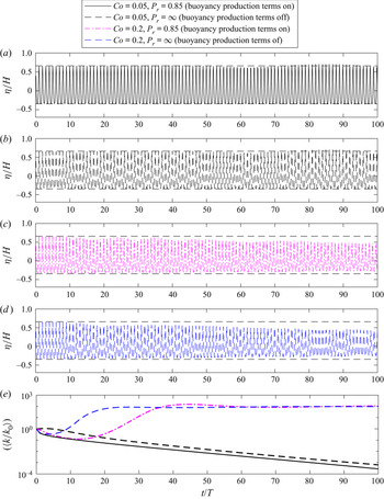
Figure 3 depicts time series of the dimensionless surface elevation as well as the period- and depth-averaged (note that $[\cdot ]$ herein indicates depth-averaging) turbulence level over a simulated duration of $100T$. It is seen in figure 3(a) that the wave propagates with nearly constant form in both cases (the two results for the free-surface elevations are indistinguishable). It is seen from figure 3(b) that the case with $\alpha _b^*=0$ results in a growth rate in the turbulent kinetic energy that may indeed be reasonably characterized as zero. This result is consistent with our simplified analysis of this problem in § 2.2, again predicting that the model is neutrally stable. Minor deviations (e.g. the initial slow decay and later rise of $[\langle k/k_0 \rangle ]$) are relatively insignificant, and are likely due to terms neglected in the analysis and/or from accumulation of small numerical errors, which may cause the solution to deviate from the ideal potential flow solution over extended times. It is likewise seen from figure 3(b) that the buoyancy production term being active instead leads to a decay in turbulence levels. This is clearly due to the additional sink in turbulence caused by this term near the air–water interface, which was not considered in the formal stability analysis. Hence, both simulations largely confirm our analysis, that the Wilcox (Reference Wilcox2006) stress–$\omega$ model is indeed stable in the ideal potential flow core region beneath non-breaking surface waves. Note that both results presented in figure 3 differ considerably from the simulation using the Wilcox (Reference Wilcox2006) $k$–$\omega$ closure model in its standard form, as presented in figure 4(a) of Larsen & Fuhrman (Reference Larsen and Fuhrman2018), which resulted in immediate exponential growth of the eddy viscosity (hence turbulence) and eventual wave decay, due to this model's inherent instability, as shown and discussed therein.

Figure 3. Computed (a) surface elevation time series and (b) the time- and depth-averaged turbulence level for the progressive waves with the Wilcox (Reference Wilcox2006) stress–$\omega$ model, with buoyancy production term both off ($\alpha _b^*=0$) and on ($\alpha _b^*=1.36$).

3.2. Simulating the oscillatory turbulent wave boundary layer

We now turn our attention to the performance of the Wilcox (Reference Wilcox2006) stress–$\omega$ model in the bottom boundary layer region beneath waves, an area of special importance beneath both non-breaking and breaking waves. (Recall that this region was neglected in the previous wave train simulations due to the use of a slip condition at the sea bed.) For this purpose, we consider the experiments of Jensen, Sumer & Fredsøe (Reference Jensen, Sumer and Fredsøe1989) conducted in a full-scale oscillating tunnel facility. We specifically consider their Test 13, involving the boundary layer beneath a sinusoidally varying free-stream flow (having velocity magnitude $U_{0m}=2.0\ \textrm {m}\ \textrm {s}^{-1}$ and period $T=9.72$ s) yielding a Reynolds number $Re=aU_{0m}/\nu \approx 6\times 10^6$, where $a=U_{0m}/\sigma _w$ and $\nu =1.14 \times 10^{-6}\ \textrm {m}^2\ \textrm {s}^{-1}$. The bottom wall is rough, with Nikuradse's equivalent roughness $k_s=0.84$ mm. A model height of 0.145 m corresponding to half of the physical tunnel height (0.29 m) in Jensen et al. (Reference Jensen, Sumer and Fredsøe1989) is used, hence only the bottom boundary layer is simulated. The top boundary is treated as a frictionless (slip) lid. The bottom boundary is set as a no-slip wall, where the $\omega$ wall function with a viscous–inertial sublayer blending method (Menter & Esch Reference Menter and Esch2001; Popovac & Hanjalic Reference Popovac and Hanjalic2007) is applied, combined with a zero normal gradient condition for the Reynolds stress. The first cell centre near the bottom wall lies at $y_c/k_s=0.5$. An oscillatory body force is applied to drive the flow until an equilibrium (periodic in time) state is reached and comparisons are made.

Computed and experimental results are compared in figure 4 at four phases during the oscillation cycle: $\sigma _w t=0^\circ$ (free-stream flow reversal), $45^\circ$ (flow acceleration due to a favourable pressure gradient), $90^\circ$ (peak free-stream flow) and $135^\circ$ (flow deceleration due to an adverse pressure gradient). Results are shown for the dimensionless mean flow $\bar {u}/U_{0m}$ (figure 4a); the turbulent kinetic energy density $k/U_{0m}^2$ (figure 4b), which for the experiments of Jensen et al. (Reference Jensen, Sumer and Fredsøe1989) has been empirically approximated from (Justesen Reference Justesen1991)

(3.3)\begin{equation} k={-}0.65(\tau_{11} + \tau_{22}); \end{equation}

as well as the Reynolds stress components $-\tau _{11}/U_{0m}^2$, $-\tau _{22}/U_{0m}^2$ and $\tau _{12}/U_{0m}^2$ (figures 4c, 4d and 4e, respectively). Results computed utilizing both the Wilcox (Reference Wilcox2006) stress–$\omega$ and $k$–$\omega$ models are shown, such that those of the RSM (the primary focus of the present work) may be compared directly with a simpler two-equation model. Note that for the $k$–$\omega$ model, the Reynolds stress components are obtained directly from the Boussinesq approximation (2.32).

Figure 4. Comparison of computed and measured vertical profiles for (a) $\bar {u}/U_{0m}$, (b) $\displaystyle k/U_{0m}^2$, (c) $\displaystyle -\tau _{11}/{U_{0m}^2}$, (d) $\displaystyle -\tau _{22}/U_{0m}^2$, (e) $\displaystyle \tau _{12}/U_{0m}^2$ and ( f) $\displaystyle U_{f}/U_{0m}$ for the oscillatory wave boundary layer case of Jensen et al. (Reference Jensen, Sumer and Fredsøe1989, their Test 13). The depicted CFD simulations utilize both the Wilcox (Reference Wilcox2006) stress–$\omega$ and $k$–$\omega$ turbulence models.

From figure 4(a) it is seen that the computed mean flow velocities from both models are largely similar, and in good agreement with the experiments. The most notable difference is the slight reduction (and increased accuracy) in the mean flow computed with the stress–$\omega$ model at phase $\sigma _w t=135^\circ$ (i.e. during adverse pressure and flow deceleration), relative to the $k$–$\omega$ model. This difference is explained immediately below. It is seen in figure 4(b) that the stress–$\omega$ model obviously improves the accuracy of the turbulence kinetic energy $k$, relative to the $k$–$\omega$ model, especially at phase $\sigma _w t=135^{\circ }$. Note that Sumer & Fuhrman (Reference Sumer and Fuhrman2020) have similarly documented relatively poor performance of the Wilcox (Reference Wilcox2006) $k$–$\omega$ model in simulating the deceleration stage of the wave boundary layer (see their figures 5.90–5.92), and this is a well-known deficiency with two-equation models in general (see e.g. Justesen (Reference Justesen1991) for similar finding with a $k$–$\varepsilon$ closure model). From inspection of the results just discussed in figure 4(a), it is clear that the over-prediction of $\bar {u}$ seen there with the $k$–$\omega$ model is associated with its under-prediction of $k$ at this phase, i.e. that the $k$–$\omega$ model does not extract enough energy from the mean flow during the flow deceleration stage. Since the form of the turbulence production term in the $k$ equation ($\tau _{ij}\partial \overline {u}_i/\partial {x_j}$, which simplifies to $\tau _{12}\partial \bar {u}/\partial y$ in the present horizontally uniform case) is theoretical (hence exact if its determination is free of error), it is then clear that this shortcoming must be due to inaccuracy of $\tau _{12}$ from the Boussinesq approximation (2.32).

The individual Reynolds stress component profiles at each stage are presented in figure 4(c–e). It is seen that the stress–$\omega$ model captures the dynamics of both the turbulent normal and shear stress components with better accuracy compared to the $k$–$\omega$ model, although $\tau _{11}$ and $\tau _{12}$ at $\sigma _w t=135 ^{\circ }$ are still slightly under-predicted in the near-bottom region. It is seen in figure 4(c,d) that $\tau _{11}$ and $\tau _{22}$ predicted by the $k$–$\omega$ model (blue dashed lines) are identical and deviate from the experimental measurements. This is simply because application of the Boussinesq approximation (2.32) for the present case leads simply to

(3.4a,b)\begin{equation} \tau_{11}= \tau_{22} ={-}\frac{2}{3}k, \quad \tau_{12} = \nu_t \frac{\partial \bar{u}}{\partial y}, \end{equation}

the former of which is well known to be incorrect, even in the simpler case of a steady horizontally uniform turbulent boundary layer flow; see e.g. Chapter 3 of Sumer & Fuhrman (Reference Sumer and Fuhrman2020). In line with the discussion above, it is notable that $\tau _{12}$ (figure 4e) is indeed under-predicted by the $k$–$\omega$ model at $\sigma _wt=135^\circ$. Overall, the Wilcox (Reference Wilcox2006) stress–$\omega$ model is demonstrated to be superior to the $k$–$\omega$ model in simulating the turbulence dynamics for the oscillatory wave boundary layer flows, as measured by Jensen et al. (Reference Jensen, Sumer and Fredsøe1989).

The measured and modelled friction velocity $U_f$ is likewise presented in figure 4(f). In the experiment of Jensen et al. (Reference Jensen, Sumer and Fredsøe1989), the friction velocity was determined by fitting straight lines to the logarithmic-layer portion of the mean velocity distribution (see Sumer & Fuhrman Reference Sumer and Fuhrman2020, § 5.4.1). It is noted that the difference in the measurements for two half cycles are quite obvious, and are due to apparent asymmetries that occurred in the experiment, which are avoided in the numerical simulations. It is seen that both stress–$\omega$ and $k$–$\omega$ model results match the friction velocity closely for the first half cycle. The friction velocity simulated with the stress–$\omega$ model is identical to that with the $k$–$\omega$ model in the flow acceleration stage, while being slightly larger than that with the $k$–$\omega$ model in the peak and deceleration stages. As the difference in the measurements over the two half cycles is larger than that of the two numerical results, both numerical model results are considered acceptable.

3.3. Simulating spilling breaking waves

The preceding preliminary simulations have demonstrated potential advantages of using a stress–$\omega$ model (rather than a traditional two-equation $k$–$\omega$ turbulence closure) for applications relevant to non-breaking waves, ranging from the free surface (the progressive wave train) to the sea bottom (the turbulent wave boundary layer). Let us now apply the model to simulate breaking wave hydrodynamics, the primary aim of the present paper. For this purpose, we first consider the spilling breaking wave experiment of Ting & Kirby (Reference Ting and Kirby1994, Reference Ting and Kirby1996), to be followed by their plunging breaking wave experiment in the following subsection.

The numerical set-up for simulation of the experiments of Ting & Kirby (Reference Ting and Kirby1994, Reference Ting and Kirby1996) is shown in figure 5, where a $\tan \beta =1/35$ constant slope is connected to a region having constant still water depth $h_0=0.4$ m. The origin is placed at the same water depth ($h=0.38$ m) as in the experiments, for consistency. A relaxation zone (Jacobsen et al. Reference Jacobsen, Fuhrman and Fredsøe2012) of one wavelength is set at the inlet for wave generation, which also serves to absorb any reflected waves. A no-slip condition along with standard smooth bed wall functions are employed as the bottom boundary conditions, since in the experiments of Ting & Kirby (Reference Ting and Kirby1994) and Ting & Kirby (Reference Ting and Kirby1996) a roughness value was not explicitly indicated. The computational mesh utilized is identical to that used previously by Larsen & Fuhrman (Reference Larsen and Fuhrman2018). Dimensional and dimensionless wave properties utilized for the simulation of both spilling and plunging breaking wave cases are indicated in table 1, where a numerically exact stream function (potential flow) theory is used for specification of the generated wave at the inlet. In table 1, $x_b$ denotes the position of incipient breaking and

(3.5)\begin{equation} \xi_0=\frac{\tan\beta}{\sqrt{H_0/L_0}} \end{equation}

is the surf similarity parameter, where $L_0=gT^2/(2{\rm \pi} )$ is the deep-water wavelength and

(3.6)\begin{equation} H_0 = H\sqrt{\tanh(k_wh)\left(1+\frac{2k_wh}{\sinh(2k_wh)}\right)} \end{equation}

is the deep-water wave height, calculated according to linear wave theory. The breaking wave simulations are initially run for $50T$ to reach equilibrium, followed by a subsequent $50T$ which is utilized for period-averaging purposes. The simulated spilling breaking case with the stress–$\omega$ model required approximately 12 days to run in parallel on 16 processors on the supercomputing cluster at the Technical University of Denmark (DTU). Note that the total computational time using the stress–$\omega$ model is approximately 15 % more than that using the $k$–$\omega$ model.

Figure 5. Computational domain set-up for plunging and spilling breaker cases corresponding to the breaking wave experiments of Ting & Kirby (Reference Ting and Kirby1994).

Table 1. Wave properties for breaking wave simulations. Parameter $x_b$ is the measured breaking point in Ting & Kirby (Reference Ting and Kirby1994) and $\xi _0$ is the surf similarity parameter.

To elucidate differences between the Wilcox (Reference Wilcox2006) stress–$\omega$ and two-equation $k$–$\omega$ turbulence closure models, simulations utilizing a stabilized version of the Wilcox (Reference Wilcox2006) $k$–$\omega$ model, as proposed by Larsen & Fuhrman (Reference Larsen and Fuhrman2018) (with stress-limiter coefficients $\lambda _1=0.2$ and $\lambda _2=0.05$, as suggested there and in their notation), are also considered for comparison. This model will hereafter be called the LF18 $k$–$\omega$ model. Note that results based on the LF18 $k$–$\omega$ model have been re-simulated for presentation herein, to ensure full consistency with the stress–$\omega$ results. This ensures that any effects associated, for example, with the specific OpenFOAM software version or boundary treatment are fully controlled for. (Such effects have not been found to be very significant, but this accounts for subtle differences in the results presented herein compared to those originally presented in Larsen & Fuhrman (Reference Larsen and Fuhrman2018).)

To begin our investigation, figure 6 depicts a snapshot of the spilling breaker turbulent kinetic energy (here presented dimensionless as $k/(gh_0)$, where $h_0=0.4$ m is the constant still water depth prior to the slope) simulated with the Wilcox (Reference Wilcox2006) stress–$\omega$ model at $t/T=100$. It is observed that there is no sign of turbulence over-production prior to breaking, indicating that the Wilcox (Reference Wilcox2006) stress–$\omega$ model is indeed stable, i.e. free of unphysical exponential growth of turbulence in nearly potential flow regions. This is once again consistent with our analysis of this model (§ 2) as well as our previous CFD simulations involving a progressive wave train (§ 3.1). The present result is in stark contrast to those stemming from two-equation models (both $k$–$\omega$ and $k$–$\varepsilon$ variants) in their standard forms; see e.g. Brown et al. (Reference Brown, Greaves, Magar and Conley2016), Larsen & Fuhrman (Reference Larsen and Fuhrman2018, their figure 6a,b), Larsen et al. (Reference Larsen, van der A, van der Zanden, Ruessink and Fuhrman2020) and Fuhrman & Li (Reference Fuhrman and Li2020, their figure 7a).

Figure 6. Snapshot of the spilling breaker turbulent kinetic energy simulated with the Wilcox (Reference Wilcox2006) stress–$\omega$ model at $t/T=100$.

Figure 7 shows the surface elevation envelopes for the spilling breaker simulations, where $\langle \eta \rangle$ is the period-averaged mean water level (over the final 50$T$), and $\eta _{max}$ and $\eta _{min}$ are respectively the averaged maximum and minimum surface elevations. Results from both the stress–$\omega$ and LF18 $k$–$\omega$ models are shown separately. The grey shaded regions depict plus and minus one standard deviation, hence indicating the degree of wave-to-wave variability. Good agreement is observed in figure 7(a) between the simulation with the Wilcox (Reference Wilcox2006) stress–$\omega$ model and the measurements of Ting & Kirby (Reference Ting and Kirby1994). The predicted breaking point (where $\eta _{max}-\langle \eta \rangle$ is the highest) is consistent with the experimental measurement. The surface elevation envelopes predicted by the LF18 $k$–$\omega$ model are also similarly in line with the experimental measurement (figure 7b), consistent with previous demonstrations.

Figure 7. Period-averaged surface elevation envelopes for the spilling breaker simulated with (a) the Wilcox (Reference Wilcox2006) stress–$\omega$ model and (b) the LF18 $k$–$\omega$ model, comparing with the experimental measurement of Ting & Kirby (Reference Ting and Kirby1994). Grey shaded areas are the plus and minus one standard deviation.

Figure 8(a–d) compares the computed phase-averaged surface elevations with the experimental measurements of Ting & Kirby (Reference Ting and Kirby1994) at four post-breaking cross-shore locations, where $\bar {\eta }$ denotes the phase-averaged surface elevation and $\langle \eta \rangle$ denotes the period-averaged surface elevation. Additionally, the two model results are compared even further onshore ($x=9.725$ m) in figure 8(e), for completeness. (Although the phase-averaged surface elevations from the experiments were not directly reported at this position, velocity and turbulence profiles were, to be presented in what follows.) It is seen that the numerical predictions with both turbulence models are generally in line with the experimental data for the three positions furthest offshore (figure 8a–c). Further onshore, the stress–$\omega$ model maintains this accuracy. However, it is seen in figure 8(d,e) that the wave front computed with the LF18 $k$–$\omega$ model is well ahead of what was measured. This was also noticed by Larsen & Fuhrman (Reference Larsen and Fuhrman2018), indicating that the breaking bore travels too rapidly in the inner surf zone. Larsen & Fuhrman (Reference Larsen and Fuhrman2018) (see their figure 10) showed clearly that this problem was due to the conventional stress-limiter on the eddy viscosity (controlled by the $\lambda _1$ coefficient in their notation) within the Wilcox (Reference Wilcox2006) $k$–$\omega$ model. Simulations where this feature was on ($\lambda _1>0$) resulted in significantly improved results (in terms of undertow velocity and turbulence profiles) in the outer surf zone, but at the expense of reduced accuracy in the inner surf zone. The stress–$\omega$ model, on the other hand, breaks free of the eddy viscosity concept altogether, and hence avoids this issue entirely.

Figure 8. Phase-averaged surface elevation for the spilling breaker from the experimental measurement of Ting & Kirby (Reference Ting and Kirby1994) and the present simulations. (a–c) The outer surf zone; (d,e) the inner surf zone.

Let us now turn our attention to the turbulence quantities beneath the spilling breaking waves. Ting & Kirby (Reference Ting and Kirby1994, Reference Ting and Kirby1996) have reported results for $\sqrt {\langle k\rangle }$, $\langle \sqrt {-\tau _{11}} \rangle$ and $\langle \tau _{22}\rangle /\langle \tau _{11}\rangle$ at each measurement position. Although the measurements for $\langle \tau _{22}\rangle$ were not directly reported, they can be obtained from their reported $\sqrt {\langle k\rangle }$ and $\langle \tau _{22}\rangle /\langle \tau _{11}\rangle$ values. In Ting & Kirby (Reference Ting and Kirby1994), because the transverse velocity component was not measured, $k$ was estimated empirically by

(3.7)\begin{equation} \left\langle k \right\rangle = \tfrac{-1.33}{2}\left( \langle \tau_{11}\rangle+\langle \tau_{22}\rangle \right), \end{equation}

which is also utilized for the experimental $k$ values presented in what follows. For the LF18 $k$–$\omega$ model, the Reynolds stress components are again obtained directly from the Boussinesq approximation (2.32).

Figures 9 and 10 compare specific period-averaged Reynolds normal stress (non-dimensionalized $-\tau _{11}=\overline {u^\prime u^\prime }$ and $-\tau _{22}=\overline {v^\prime v^\prime }$ period-averaged over the final simulated $50T$; results are similarly period-averaged in several forthcoming figures) profiles at each of the measured cross-shore positions. Figure 11 similarly presents a comparison of computed and measured period-averaged turbulent kinetic energy density $k$ profiles. From these figures, it can be surmised that both the Wilcox (Reference Wilcox2006) stress–$\omega$ model and the LF18 $k$–$\omega$ model predict Reynolds normal stress components that are reasonably, though not perfectly, in line with the measurements. It is noted that the stress–$\omega$ model predicts streamwise normal stresses ($\tau _{11}$) significantly better than vertical ones ($\tau _{22}$). This might be attributed to the simple formulation of pressure–strain closure in the Wilcox (2006) stress–$\omega$ model, as the streamwise normal stresses ($\tau _{11}$) are dominated by the production term $P_{11}$ while $\tau _{22}$ is mainly driven by the pressure–strain correlation $\varPi _{22}$. It is seen in figure 11(d–h) that there is also a tendency for the LF18 $k$–$\omega$ model to predict more accurate turbulence near the free surface, where the stress–$\omega$ model predicts slightly higher turbulence than the $k$–$\omega$ model. This can also be attributed to the standard Wilcox (Reference Wilcox2006) stress-limiting feature in the $k$–$\omega$ model, as shown through systematic testing by Larsen & Fuhrman (Reference Larsen and Fuhrman2018, compare e.g. Cases 3 and 5 in their figure 12).

Figure 9. Period-averaged Reynolds normal stress $-\tau _{11}$ for the spilling breaker from the experimental measurement of Ting & Kirby (Reference Ting and Kirby1994) and the present simulations. (a,b) The pre-breaking region; (c–e) the outer surf zone; ( f–h) the inner surf zone.

Figure 10. Period-averaged Reynolds normal stress $-\tau _{22}$ for the spilling breaker from the experimental measurement of Ting & Kirby (Reference Ting and Kirby1994, Reference Ting and Kirby1996) and the present simulations.

Figure 11. Period-averaged turbulent kinetic energy $k$ for the spilling breaker from the experimental measurement of Ting & Kirby (Reference Ting and Kirby1994) and the present simulations.

Let us now similarly investigate the computed Reynolds shear stresses $\tau _{12}=-\overline {u^\prime v^\prime }$, which can be expected to play a much more important role in terms of flow resistance than the turbulent normal stresses. Figure 12 compares the period-averaged $\tau _{12}$ (again over the final simulated $50T$) profiles from both models at all eight measurement positions considered previously. Note that this quantity was not reported by Ting & Kirby (Reference Ting and Kirby1994), and thus we are not able to compare directly with their measurements; nevertheless, important differences between the two models are revealed. It is seen from figure 12(a–d) that neither model predicts significant Reynolds shear stress prior to breaking (as should be expected) or in the outer surf zone. However, further shoreward the Reynolds shear stress predicted with the Wilcox (Reference Wilcox2006) stress–$\omega$ model is significantly larger than with the LF18 $k$–$\omega$ model, particularly in the upper part of the water column i.e. near the surface. These differences can also be seen directly in figure 13, which compares (phase-averaged) snapshots of the specific Reynolds shear stress ($\tau _{12}$) field beneath breaking bores computed with both models in the inner surf zone. The instant shown has been selected such that the surface breaking wave front is approximately at the innermost measurement position ($x=9.725$ m). The increased Reynolds shear stresses with the stress–$\omega$ model will in turn increase flow resistance in the upper part of the water column. Although we again cannot compare directly with measurements of $\tau _{12}$ in the present case, it is now evident that it is this increased flow resistance that is responsible for slowing the propagation of the breaking wave front in the inner surf zone, bringing the resulting (phase-averaged) surface elevation time series computed with the stress–$\omega$ model in line with that measured (see again e.g. figure 8d). In Larsen & Fuhrman (Reference Larsen and Fuhrman2018), the flow resistance was represented through the eddy viscosity $\nu _t$, as shown in their figure 14. A higher eddy viscosity in the upper part of the flow extracts more energy from the mean flow, which reduces the mean flow velocities. However, the stress–$\omega$ model does not utilize the eddy viscosity assumption. Therefore, we compare the flow resistance between two turbulence models through $P_k$, as given in (2.31) and (2.33a,b), which represents the rate at which kinetic energy is transferred from the mean flow to the turbulence (Wilcox Reference Wilcox2006, p. 109). For the stress–$\omega$ model, the turbulence shear production is in the form of $\tau _{12} S_{12}$ which is seen to be the rate at which work is done by the mean shear strain rate against the Reynolds shear stress. Therefore, $P_k$ is an indicator of flow resistance that is induced by the Reynolds shear stress $\tau _{12}$. For the two-equation model, $P_k$ is calculated based on $\nu _t$, as is presented in (2.33a,b). As shown in figure 14 in the upper part of the flow (right beneath the breaking bore), the shear production of turbulence with the stress–$\omega$ model is larger than with LF18 $k$–$\omega$ model, indicating higher flow resistance near the broken wave surface with the stress–$\omega$ model. The related effects on the period-averaged undertow velocity profiles are considered in the next paragraph.

Figure 12. Period-averaged specific Reynolds shear stress $\tau _{12}$ for the spilling breaker from the experimental measurement of Ting & Kirby (Reference Ting and Kirby1994) and the present simulations.

Figure 13. Phase-averaged $\tau _{12}$ at $t/T=0.08$ for the spilling breaker case computed with the (a) Wilcox (Reference Wilcox2006) stress–$\omega$ model and (b) LF18 $k$–$\omega$ model. Results are scaled using the depth $h=0.102$ m at $x=9.725$ m.

Figure 14. Period-averaged $P_k$ for the spilling breaker from the present simulations.

As hinted immediately above, figure 15 compares computed and measured period-averaged undertow velocity profiles. It is seen that the stabilized LF18 $k$–$\omega$ model provides accurate undertow velocity profiles before wave breaking and in the outer surf zone (figure 15a–e), generally consistent with the earlier findings of Larsen & Fuhrman (Reference Larsen and Fuhrman2018). Once reaching the inner surf zone (figure 15f–h), however, the LF18 $k$–$\omega$ model yields exaggerated undertow velocities. In contrast, the stress–$\omega$ model maintains consistent accuracy in the computed undertow velocity profile across the entirety of the measured surf zone, resulting in a significant increase in accuracy. These differences seem clearly linked to the increased flow resistance near the surface shown in figure 12(e–h) and figure 13, and the related increased accuracy of the breaking bore propagation evident from figure 8(d). As the Reynolds shear stress in two-equation turbulence closure models is computed based on the Boussinesq approximation, it seems clear that this classical assumption utilized within two-equation models (even in their stabilized form) fails to yield the correct evolution of the flow resistance in the inherently complicated inner surf zone, which further leads to locally inaccurate undertow predictions.

Figure 15. Period-averaged undertow velocity profiles for the spilling breaker from the experimental measurement of Ting & Kirby (Reference Ting and Kirby1994) and the present simulations.

The accurate prediction of undertow velocities is of major importance in the fluid mechanics of the surf zone, as they are important drivers of fluid, pollutants and sediment transport in nearshore coastal regions. Despite this importance, the problem of inaccurate undertow velocity profiles has consistently plagued RANS CFD simulations of breaking waves over the past two decades. The present results utilizing the Wilcox (Reference Wilcox2006) stress–$\omega$ model are novel, in that they represent the first time that consistent quantitative accuracy in the computed undertow has been maintained throughout the entirety of the nearshore wave breaking process, i.e. during shoaling (prior to breaking), to the outer surf zone and all the way into the inner surf zone. Other RANS models (typically using two-equation turbulence closure) yield incorrect undertow structure prior to breaking and in the outer surf zone (e.g. Lin & Liu Reference Lin and Liu1998; Brown et al. Reference Brown, Greaves, Magar and Conley2016; Devolder et al. Reference Devolder, Troch and Rauwoens2018; Liu et al. Reference Liu, Ong, Obhrai, Gatin and Vukčević2020) or exaggerated undertow in the inner surf zone (e.g. Jacobsen et al. Reference Jacobsen, Fuhrman and Fredsøe2012; Larsen & Fuhrman Reference Larsen and Fuhrman2018; Larsen et al. Reference Larsen, van der A, van der Zanden, Ruessink and Fuhrman2020), or both. A detailed discussion of the results and problems in previous works is presented in § 4.

3.4. Simulating plunging breaking waves

We now employ the Wilcox (Reference Wilcox2006) stress–$\omega$ model to simulate the plunging breaking wave experiments of Ting & Kirby (Reference Ting and Kirby1994, Reference Ting and Kirby1996). For these simulations the numerical set-up and protocol are identical to that used for spilling breakers in § 3.3, with the wave parameters as indicated in table 1. The simulation of the plunging breaking waves required approximately 25 days to run in parallel on 16 processors on the supercomputing cluster at DTU. As before, comparison is made with the LF18 $k$–$\omega$ model (Larsen & Fuhrman Reference Larsen and Fuhrman2018), which again represents a stabilized form of the basic model presented by Wilcox (Reference Wilcox2006). As much of the story to follow bears similarity to that in § 3.3, it will be told with far greater brevity in the present subsection.

Figure 16 depicts a snapshot of the dimensionless turbulence field $k/(\omega \nu )$ for the plunging breaking case, computed with the stress–$\omega$ model at a time instant of $t/T=50.825$, similar to figure 6. This time instant has been chosen, as it corresponds to wave over-turning just prior to the subsequent plunge. Similar to our findings in the spilling breaking case, there is no turbulence over-production prior to wave breaking. This should by now be expected as we have definitively established that the stress–$\omega$ model is stable in nearly potential flow regions beneath surface waves. It can be noted that this plunging case is not nearly as prone to significant turbulence over-production prior to breaking as the spilling case, because the unstable growth rate is much smaller due to a small value of $[\langle p_0 \rangle ]$, as discussed by Larsen & Fuhrman (Reference Larsen and Fuhrman2018).

Figure 16. Snapshot of the plunging breaker turbulent kinetic energy simulated with the Wilcox (Reference Wilcox2006) stress–$\omega$ model at $t/T=100$.

Figure 17 compares the surface elevation envelopes from the model simulations with the experimental measurements, similar to figure 7. A reasonable match is again achieved. Both the Wilcox (Reference Wilcox2006) stress–$\omega$ and LF18 $k$–$\omega$ models predict the breaking point, and subsequent wave decay, reasonably. The set-up in the mean water level is likewise similarly well predicted. It is noted that right after the breaking point (at $x \approx 8$ m), the maximum surface elevation predicted with both numerical models has small deviations from the experimental measurement (with the stress–$\omega$ model result being slightly closer to the measurement). This deviation could be due to the plunging jet splashing down and causing turbulent mixture of the surface layer (as discussed in Brocchini (Reference Brocchini2002)) which makes accurate modelling challenging. However, our numerical models are able to show reasonable consistency with the measurements, with minor deviations in the splash region. Comparisons of computed and measured phase-averaged time series of the surface elevation at several measurement positions are additionally provided in figure 18. Interestingly, apart from the deviations near the crest in figure 18(c–e) with the $k$–$\omega$ model, the computed wave front in the present plunging case does not propagate noticeably faster with the $k$–$\omega$ model in the inner surf zone. This differs from our findings in the spilling case (see figure 8d,e), and is explained later in this subsection.

Figure 17. Surface elevation envelopes for the plunging breaker simulated with (a) the present Wilcox (Reference Wilcox2006) stress–$\omega$ model and (b) the LF18 $k$–$\omega$ model, comparing with the experimental measurement of Ting & Kirby (Reference Ting and Kirby1994). Grey shaded areas are the plus and minus one standard deviation.

Figure 18. Phase-averaged surface elevation for the plunging breaker from the experimental measurement of Ting & Kirby (Reference Ting and Kirby1995) and the present simulations. (a–c) The outer surf zone; (d,e) the inner surf zone.

Computed and measured (when available) period-averaged (over the final $50T$, as before) turbulent normal stress profiles are compared in figures 19 (for $-\tau _{11}$) and  20 (for $-\tau _{22}$), with profiles for the turbulent kinetic energy density $k$ similarly presented in figure 21. In the experiments, $k$ was again estimated from (3.7). As Ting & Kirby (Reference Ting and Kirby1994) did not provide measurement data for $\langle -\tau _{22}\rangle$ or $\langle \tau _{22}\rangle /\langle \tau _{11}\rangle$ for their plunging case, only model results are shown in figure 20. From these figures it is seen that the two models seem to provide comparable accuracy for the turbulent normal stresses, similar to what was shown in our prior simulations involving spilling breaking waves. The results for $k$ are somewhat more accurate with the stress–$\omega$ model specifically at $x=9.795$ m (figure 21g), though this increased accuracy is not consistent throughout the surf zone as a whole. The overall predictions for $k$ in the inner surf zone with both turbulence models are larger than the measurement with a maximum factor of two (figure 21g). The reason remains uncertain to the authors. However, it is worthwhile to mention that the experimental study of Scott et al. (Reference Scott, Cox, Maddux and Long2005) presented $k$ profiles post-processed with three different turbulence separation methods, with results varying by up to a factor of two to six from one another. The vertical gradient of their largest prediction is much higher than that of the lowest prediction (as shown in their figure 5). Therefore, the difference between our numerical results and the measurement of Ting & Kirby (Reference Ting and Kirby1994) might still be considered reasonable.

Figure 19. Period-averaged specific Reynolds normal stress $-\tau _{11}$ profiles for the plunging breaker from the experimental measurement of Ting & Kirby (Reference Ting and Kirby1994) and the present simulations. (a,b) The pre-breaking region; (c–e) the outer surf zone; ( f–h) the inner surf zone.

Figure 20. Period-averaged specific Reynolds normal stress $-\tau _{22}$ profiles for the plunging breaker from the present simulations.

Figure 21. Period-averaged turbulent kinetic energy $k$ profiles for the plunging breaker from the experimental measurement of Ting & Kirby (Reference Ting and Kirby1994) and the present simulations.

Figure 22 presents the computed phase-averaged $\tau _{12}$ field in the surf zone for the plunging case with both models, in a fashion similar to figure 13. The phase plotted has been selected to capture the propagation of the breaking wave front in the inner surf zone. Similar to our findings in the spilling case, it is clearly seen that the stress–$\omega$ model predicts turbulent shear stresses that are significantly larger in the inner surf zone than that with the $k$–$\omega$ model. It can thus be expected to result in increased flow resistance in this region. From comparison of figures 22 and 13 it is also seen that the increased turbulent shear stresses in the plunging case are spread more uniformly throughout the water column than in the spilling case, where they were more concentrated near the surface. This is likely due to the more violent surf zone initiated by the plunging breaking, and thus also explains why the breaking surface front propagates at approximately the same speed in the inner surf zone with both models in the present case (see again figure 18). The flow resistance indicated by $P_k$ for the plunging breaker is likewise presented in figure 23. It is clearly seen that in the upper part of the flow, $P_k$ predicted with the stress–$\omega$ model is much larger than that predicted with the LF18 $k$–$\omega$ model, indicating higher flow resistance and therefore smaller magnitude of mean flow velocity with the stress–$\omega$ model.

Figure 22. Phase-averaged $\tau _{12}$ at $t/T=0.30$ for the plunging breaker case computed with the (a) Wilcox (Reference Wilcox2006) stress–$\omega$ model and (b) LF18 $k$–$\omega$ model. Results are scaled using the depth $h=0.083$ m at $x=10.395$ m.

Figure 23. Period-averaged $P_k$ for the plunging breaker from the present simulations.

Figure 24 finally compares computed and measured undertow velocity profiles. It is seen that before wave breaking (figure 24a–c), the numerical simulations with both turbulence models are almost identical, and are in line with the experimental measurement. This is as expected, since both model variants considered herein are formally stable in the potential flow regions beneath surface waves; hence the choice of turbulence model has little impact prior to breaking. Results are also similar in the outer surf zone, as seen in figure 24(d,e). Much more significant differences become apparent once the inner surf zone is reached, as seen in figure 24( f–h). Consistent with the previously considered spilling breaking case (figure 15), in the inner surf zone the LF18 $k$–$\omega$ model results in undertow velocity profiles that are much larger than were measured. The LF18 turbulence model similarly yielded over-predicted undertow velocities in the simulation of large-scale plunging breakers made by Larsen et al. (Reference Larsen, van der A, van der Zanden, Ruessink and Fuhrman2020). It is thus now evident that this is a consistent shortcoming with this model, which stems from the inclusion of the traditional stress-limiter within the Wilcox (Reference Wilcox2006) $k$–$\omega$ model (see again the comparisons made by Larsen & Fuhrman (Reference Larsen and Fuhrman2018), with this feature switched on and off). The stress–$\omega$ model, on the other hand, reduces this exaggeration considerably, though not completely. The undertow profiles predicted with this model in the inner surf zone are much more uniform, having a similar structure to what has been measured. The reduction in the undertow magnitudes computed with the stress–$\omega$ model is consistent with the increased flow resistance in the inner surf zone, as illustrated in figures 22 and 23.

Figure 24. Period-averaged undertow velocity profiles for the plunging breaker from the experimental measurement of Ting & Kirby (Reference Ting and Kirby1994) and the present simulations.

Though a substantial improvement of the predicted undertow in the inner surf zone is seen with the stress–$\omega$ model, there are still some disagreements between the stress–$\omega$ model prediction and the experimental measurement for the plunging breaker (figure 24f–h). The reasons are, as yet, uncertain to the authors. One possible reason could be the simplistic formulation of the pressure–strain terms in the Wilcox (Reference Wilcox2006) stress–$\omega$ model, for which more complex closures for pressure–strain terms could potentially make further improvement for the undertow predictions in the complicated inner surf zone of plunging breakers. Another possible reason could be air bubbles entrained in the plunging surf zone. The present study has not specifically employed a model for the air bubbles/pockets. The bubble-mass cascade phenomena (Chan et al. Reference Chan, Johnson, Moin and Urzay2021) and the bubble breakup in the inner surf zone may further increase the flow resistance. These may be interesting to investigate in future work.