2.1 Laminar velocity profiles

The non-dimensional velocity profile for laminar Couette flow is $U(z)=z$; for laminar Poiseuille flow it is $U(z)=1-z^{2}$. Linearizing the incompressible Navier–Stokes equations about one of these laminar base flows gives

(2.1a)$$\begin{eqnarray}\displaystyle & \displaystyle \frac{\unicode[STIX]{x2202}\boldsymbol{u}}{\unicode[STIX]{x2202}t}+U\frac{\unicode[STIX]{x2202}\boldsymbol{u}}{\unicode[STIX]{x2202}x}+(wU^{\prime },0,0)=-\unicode[STIX]{x1D735}p+R^{-1}\unicode[STIX]{x0394}\boldsymbol{u}+\boldsymbol{f}, & \displaystyle\end{eqnarray}$$

(2.1b)$$\begin{eqnarray}\displaystyle & \displaystyle \unicode[STIX]{x1D735}\boldsymbol{\cdot }\boldsymbol{u}=0, & \displaystyle\end{eqnarray}$$

$\boldsymbol{u}=[u~v~w]^{\text{T}}$

$^{\prime }$

$\boldsymbol{f}=[f_{x}~f_{y}~f_{z}]^{\text{T}}$

2.2 Turbulent velocity profiles

Linear models have been used for fully developed turbulent flows in a number of previous studies. In some the linear operator is obtained from a Reynolds decomposition of the velocity field, giving rise to a linear operator in which the viscosity is equal to the kinematic viscosity (McKeon & Sharma Reference McKeon and Sharma2010; Sharma & McKeon Reference Sharma and McKeon2013). In others the linear operator is obtained by first performing a triple decomposition of the velocity field and then providing a closure for the terms quadratic in the incoherent fluctuations using a simple eddy-viscosity model (Reynolds & Hussain Reference Reynolds and Hussain1972; del Álamo & Jiménez Reference del Álamo and Jiménez2006; Pujals et al. Reference Pujals, García-Villalba, Cossu and Depardon2009; Hwang & Cossu Reference Hwang and Cossu2010a,Reference Hwang and Cossub; Illingworth, Monty & Marusic Reference Illingworth, Monty and Marusic2018; Madhusudanan, Illingworth & Marusic Reference Madhusudanan, Illingworth and Marusic2019; Vadarevu et al. Reference Vadarevu, Symon, Illingworth and Marusic2019). In this second case the effective viscosity, which varies across the flow, is given by the sum of the eddy and kinematic viscosities.

In this work we include only the kinematic viscosity in the linear model. Doing so gives rise to an Orr–Sommerfeld operator whose dynamics is independent of the mean velocity profile (to be made clear in § 2.3) and thus simpler and more generic than its eddy-viscosity equivalent. This choice is therefore convenient but it is also suitable for two reasons. First, a key emergent feature of both linear models is the critical layer mechanism in which a significant response can occur when the phase velocity, $c=\unicode[STIX]{x1D714}/k_{x}$, is equal to the local mean velocity, $c=U(z)$ (Maslowe Reference Maslowe1986). The two linear models show different critical layer behaviours owing to their different effective viscosity profiles. But since the focus of this work is on streamwise-constant fluctuations for which the streamwise wavenumber is zero, the critical layer mechanism does not occur and this difference between the two models does not exist. Second, we must specify the variation of the eddy viscosity in the wall-normal direction ($z$), but a reasonable approximation is to assume instead that it is constant with $z$. As noted by Townsend (Reference Townsend1956, § 6.7 p. 127), a reasonable way to determine this constant would be to compare the measured mean velocity profile with that given by assuming a suitable constant eddy viscosity; and the approximation would only be in error near the walls. It is therefore reasonable to approximate any eddy viscosity with an equivalent constant (and larger) viscosity which would manifest itself as a reduction in the effective Reynolds number $R$. (The effect of including an eddy viscosity in the linear model (2.1) will be considered in § 6.)

For Couette flow there is an additional reason for which the kinematic viscosity may be more appropriate than an eddy viscosity. The eddy-viscosity profile is closely related to the mean velocity profile – knowledge of one implies knowledge of the other. The strong streamwise rollers that are unique to Couette flow will surely have an influence on the mean velocity profile, and in turn on the eddy-viscosity profile. And yet the intended role of the eddy viscosity is to model the effect of small-scale, incoherent motions on the large, most energetic scales. Therefore any eddy-viscosity profile, as well as acting to modify the dynamics of the largest scales, is at the same time modified by them. This observation applies equally to Poiseuille flow and indeed any shear flow, but we can expect it to be especially problematic for Couette flow, where large-scale structures play such a prominent role.

The linear model formed about the turbulent mean flow has the same form as that for laminar flow (2.1) but the reasoning used to form it and the definition and interpretation of some its terms are different. The linear model is obtained by performing a Reynolds decomposition of the velocity field; substituting this into the incompressible Navier–Stokes equations; and subtracting the equations governing the mean flow. This gives rise to (2.1) as before but with two important differences. First, $\boldsymbol{U}$ now represents the turbulent mean velocity profile and $\boldsymbol{u}$ represents turbulent fluctuations about the mean. Second, any nonlinear terms are absorbed into the forcing term $\boldsymbol{f}$ so that $\boldsymbol{f}=-(\boldsymbol{u}\boldsymbol{\cdot }\unicode[STIX]{x1D735})\boldsymbol{u}+\overline{(\boldsymbol{u}\boldsymbol{\cdot }\unicode[STIX]{x1D735})\boldsymbol{u}}$ (Landahl Reference Landahl1967; Bark Reference Bark1975; McKeon & Sharma Reference McKeon and Sharma2010). Thus the formation of the linear operator (2.1) about the turbulent mean flow does not imply that nonlinear terms are neglected. Rather, we take the point of view that the linear operator (2.1) is constantly forced by the remaining nonlinear terms. Nonlinear effects thus manifest themselves in two ways: through their role in setting the mean velocity profile $\boldsymbol{U}$; and through their forcing of the linear operator (2.1). (The forcing could have additional contributions from any externally applied forcing as in § 2.1, but this would not modify the analysis.)

2.3 Streamwise-constant model

The streamwise-constant model used throughout this work is obtained by taking Fourier transforms of (2.1) in the homogeneous directions ($x,y$); transforming into Orr–Sommerfeld Squire form; and setting the streamwise wavenumber to zero

(2.2a)$$\begin{eqnarray}\displaystyle & \displaystyle \frac{\unicode[STIX]{x2202}\unicode[STIX]{x0394}{\hat{w}}}{\unicode[STIX]{x2202}t}=R^{-1}\unicode[STIX]{x1D6E5}^{2}{\hat{w}}-\text{i}k{\mathcal{D}}\hat{f}_{y}-k^{2}\hat{f}_{z}, & \displaystyle\end{eqnarray}$$

(2.2b)$$\begin{eqnarray}\displaystyle & \displaystyle \frac{\unicode[STIX]{x2202}\hat{u} }{\unicode[STIX]{x2202}t}=R^{-1}\unicode[STIX]{x0394}\hat{u} -U^{\prime }{\hat{w}}+\hat{f}_{x}, & \displaystyle\end{eqnarray}$$

${\hat{w}}(t)=\unicode[STIX]{x2202}_{z}{\hat{w}}(t)=\hat{u} (t)=0$

$k$

${\mathcal{D}}$

$\unicode[STIX]{x1D6E5}={\mathcal{D}}^{2}-k^{2}$

$\hat{u}$

$\hat{u}$

$\hat{\unicode[STIX]{x1D702}}$

$\hat{\unicode[STIX]{x1D702}}=\text{i}k\hat{u}$

${\hat{w}}$

$\hat{v}$

${\hat{w}}$

$\hat{u}$

$\hat{v}$

${\hat{w}}$

(2.3)$$\begin{eqnarray}\text{i}k\hat{v}+{\mathcal{D}}{\hat{w}}=0.\end{eqnarray}$$

Figure 1. Linear amplification mechanisms for streamwise-constant fluctuations at spanwise wavenumber $k$. Dashed lines denote forcing components and velocity components that are omitted in the analysis. (These processes scale with $R$, while those retained scale with $R^{2}$ – see § 2.3.) The transfer functions $G(s)$ from (2.4a) and $S(s)$ from (2.4c) are also indicated.

Taking Laplace transforms of (2.2), rescaling the Laplace variable $s$ by the Reynolds number $R$ (Gustavsson Reference Gustavsson1991; Jovanovic & Bamieh Reference Jovanovic and Bamieh2005) and rearranging gives rise to two transfer functions, $G(s)$ and $S_{o}(s)$, as follows:

(2.4a)$$\begin{eqnarray}\displaystyle & \displaystyle {\hat{w}}(s)=R\underbrace{(s\unicode[STIX]{x1D6E5}-\unicode[STIX]{x1D6E5}^{2})^{-1}\left[\begin{array}{@{}cc@{}}-\text{i}k{\mathcal{D}} & -k^{2}\end{array}\right]}_{G(s)}\left[\begin{array}{@{}c@{}}\hat{f}_{y}(s)\\ \hat{f}_{z}(s)\end{array}\right], & \displaystyle\end{eqnarray}$$

(2.4b)$$\begin{eqnarray}\displaystyle & \displaystyle \hat{u} (s)=R\underbrace{(sI-\unicode[STIX]{x1D6E5})^{-1}\left[\begin{array}{@{}cc@{}}I & -U^{\prime }\end{array}\right]}_{S_{o}(s)}\left[\begin{array}{@{}c@{}}\hat{f}_{x}(s)\\ {\hat{w}}(s)\end{array}\right]. & \displaystyle\end{eqnarray}$$

(Rescaling the Laplace variable in this way is equivalent to rescaling time by $R^{-1}$.) Notice that the Reynolds number $R$ has been isolated to render each transfer function independent of it. The transfer function $G(s)$ comes from the Orr–Sommerfeld operator. It represents the dynamics from spanwise and wall-normal forcing, $[\hat{f}_{y}~\hat{f}_{z}]^{\text{T}}$, to wall-normal velocity fluctuations, ${\hat{w}}$. Importantly, $G(s)$ is independent of the mean velocity profile. The transfer function $S_{o}(s)$ is related to the Squire operator. It represents the dynamics from streamwise forcing and wall-normal velocity fluctuations, $[\hat{f}_{x}~{\hat{w}}]^{\text{T}}$, to streamwise velocity fluctuations, $\hat{u}$. Equations (2.4) are represented in a block diagram in figure 1.

From (2.4a), (2.4b) and figure 1 we see that the overall transfer function from $[\hat{f}_{y}~\hat{f}_{z}]^{\text{T}}$ to $\hat{u}$ (which involves both $G(s)$ and $S_{o}(s)$) scales with $R^{2}$, while the transfer function from $\hat{f}_{x}$ to $\hat{u}$ (which involves only $S_{o}(s)$) scales with $R$. For sufficiently large $R$ we can therefore neglect the influence of $\hat{f}_{x}$ and it is convenient to define a second transfer function, $S(s)$, for which the influence of $\hat{f}_{x}$ is neglected

(2.4c)$$\begin{eqnarray}\hat{u} (s)=R\underbrace{[-(sI-\unicode[STIX]{x1D6E5})^{-1}U^{\prime }]}_{S(s)}{\hat{w}}(s).\end{eqnarray}$$

The transfer function $S_{o}(s)$ in (2.4b) therefore includes the influence of $\hat{f}_{x}$, while the transfer function $S(s)$ in (2.4c) neglects it.

Finally, we define an overall transfer function $F(s)$

(2.5)$$\begin{eqnarray}\displaystyle F(s) & = & \displaystyle S(s)G(s)\nonumber\\ \displaystyle & = & \displaystyle (sI-\unicode[STIX]{x1D6E5})^{-1}U^{\prime }(s\unicode[STIX]{x1D6E5}-\unicode[STIX]{x1D6E5}^{2})^{-1}\left[\begin{array}{@{}cc@{}}\text{i}k{\mathcal{D}} & k^{2}\end{array}\right].\end{eqnarray}$$

Implicit in (2.5) is that the contribution from streamwise forcing $\hat{f}_{x}$ can be ignored. This assumption is sound provided that the Reynolds number $R$ is sufficiently large, as discussed above. Then $F(s)$ represents the overall dynamics from $[\hat{f}_{y}~\hat{f}_{z}]^{\text{T}}$ to $\hat{u}$ as follows:

(2.6)$$\begin{eqnarray}\hat{u} (s)=R^{2}F(s)\left[\begin{array}{@{}c@{}}\hat{f}_{y}(s)\\ \hat{f}_{z}(s)\end{array}\right].\end{eqnarray}$$

The overall dynamics (2.6), together with definitions of $G(s)$ and $S(s)$, are shown in a block diagram in figure 1. Note that the Reynolds number scaling of the overall operator has also been analysed in the slightly different context of stochastic forcing for which the relevant norm (the two norm) is found to scale with $R^{3/2}$ (Bamieh & Dahleh Reference Bamieh and Dahleh2001; Jovanovic & Bamieh Reference Jovanovic and Bamieh2005).

2.4 Transfer function norms

With the relevant transfer functions defined, we now introduce two norms to evaluate their size: the infinity norm $\Vert \cdot \Vert _{\infty }$ and the two norm $\Vert \cdot \Vert _{2}$.

We will make extensive use of the infinity norm, defined for a transfer function $T$ as

(2.7)$$\begin{eqnarray}\Vert T\Vert _{\infty }=\max _{\unicode[STIX]{x1D714}}\,\unicode[STIX]{x1D70E}_{1}(\text{i}\unicode[STIX]{x1D714}),\end{eqnarray}$$

where $\unicode[STIX]{x1D70E}_{i}(\text{i}\unicode[STIX]{x1D714})$ are the singular values of $T(\text{i}\unicode[STIX]{x1D714})$ at frequency $\unicode[STIX]{x1D714}$ and represent a generalization of gain for systems with many inputs and many outputs. The singular values are ordered such that $\unicode[STIX]{x1D70E}_{1}\geqslant \unicode[STIX]{x1D70E}_{2}\geqslant \cdots \geqslant \unicode[STIX]{x1D70E}_{n}$. Therefore $\unicode[STIX]{x1D70E}_{1}$ represents the maximum singular value at frequency $\unicode[STIX]{x1D714}$; and the infinity norm (2.7) represents the worst-case gain over all possible forcing frequencies and forcing directions. An important property of the infinity norm – and a key reason for using it in this work – is its submultiplicative property

(2.8)$$\begin{eqnarray}\Vert T_{1}T_{2}\Vert _{\infty }\leqslant \Vert T_{1}\Vert _{\infty }\Vert T_{2}\Vert _{\infty }\end{eqnarray}$$

for any two transfer functions $T_{1}$ and $T_{2}$. This property will be useful in the following sections to characterize the efficiency of the forcing of streamwise velocity fluctuations (the Squire operator $S$) by wall-normal velocity fluctuations (the Orr–Sommerfeld operator $G$).

Another commonly used norm for transfer functions is the two norm

(2.9)$$\begin{eqnarray}\Vert T\Vert _{2}^{2}=\frac{1}{2\unicode[STIX]{x03C0}}\int _{-\infty }^{\infty }\text{Trace}[T^{\ast }(\text{i}\unicode[STIX]{x1D714})T(\text{i}\unicode[STIX]{x1D714})]\,\text{d}\unicode[STIX]{x1D714}=\frac{1}{2\unicode[STIX]{x03C0}}\int _{-\infty }^{\infty }\mathop{\sum }_{i}\unicode[STIX]{x1D70E}_{i}^{2}(\text{i}\unicode[STIX]{x1D714})\,\text{d}\unicode[STIX]{x1D714}.\end{eqnarray}$$

The two norm (2.9) represents an average gain over all frequencies and forcing directions. In contrast to the infinity norm, the two norm does not satisfy the submultiplicative property (2.8), and is therefore less suitable for our purposes (to be made clear in § 3.2). Nevertheless, it will be used briefly in § 3 to check the sensitivity of some key results to the choice of norm.

2.5 Numerical discretization

Equations (2.4a) and (2.4c) are discretized in the wall-normal direction ($z$) using Chebyshev collocation. A total of 101 Chebyshev points are used, which is sufficient for the large scales of interest. Convergence has been checked by doubling the number of Chebyshev points and ensuring that the results do not change. The norms (2.7) and (2.9) are defined such that they each correspond to grid-independent energy norms. This is achieved using Clenshaw–Curtis quadrature (Trefethen Reference Trefethen2008).

3.1 Norms of $G$, $S$ and $F$ with spanwise wavenumber

Figure 2 plots the infinity norm (2.7) as a function of spanwise wavenumber for $G$, $S$ and $F$. We plot all norms only for non-zero values of $k$ since, when $k=0$, the continuity equation becomes simply $\unicode[STIX]{x2202}w/\unicode[STIX]{x2202}z=0$, which, together with the boundary conditions for $w$, implies that $w=0$ everywhere. Recall from § 2.3 that the Reynolds number $R$ has been isolated from each transfer function (see (2.4) and (2.6)). This means that all results effectively correspond to $R=1$. This, coupled with the fact that the infinity norm satisfies $\Vert RT(s)\Vert _{\infty }=R\Vert T(s)\Vert _{\infty }$ for any transfer function $T(s)$ (and $R$ positive), means that the results at any Reynolds number can be readily generated from the results presented here. The infinity norm of the Orr–Sommerfeld operator $G$ is plotted in figure 2(a). Recall that, for streamwise-constant fluctuations, the dynamics of $G$ is independent of the mean velocity profile and is therefore identical for Poiseuille flow and Couette flow. We observe that $\Vert G\Vert _{\infty }$ attains its maximum at a spanwise wavenumber of $k=2.00$ ($\unicode[STIX]{x1D706}=3.14$). The infinity norm of the Squire operator $S$ is plotted in figure 2(b). Notice that there are now two curves – one for Couette flow and one for Poiseuille flow – because $S$ is a function of the mean velocity profile. For both flows $\Vert S\Vert _{\infty }$ attains its maximum at $k=0$ and decreases monotonically with increasing $k$. Finally, the infinity norm of $F=SG$, which represents the overall dynamics, is plotted in figure 2(c). For both flows $\Vert F\Vert _{\infty }$ attains its maximum near $k\approx \unicode[STIX]{x03C0}/2$ ($\unicode[STIX]{x1D706}\approx 4$). Precisely, $\Vert F\Vert _{\infty }$ attains its maximum at $k=1.18$ ($\unicode[STIX]{x1D706}=5.3$) for Couette flow and at $k=1.62$ ($\unicode[STIX]{x1D706}=3.9$) for Poiseuille flow.

Figure 2. The infinity norm $\Vert \cdot \Vert _{\infty }$ for $G$ (a); $S$ (b); and $F=SG$ (c). Results for $S$ and $F$ are shown for Couette flow (——) and for Poiseuille flow (– –).

What if we use a different norm? Table 1 summarizes the spanwise wavenumbers at which the peak response, as measured by the infinity norm, is achieved; and also repeats this using the two norm (2.9). (The variation of the two norm with $k$ is plotted in the Appendix.) When rescaled by $R$, the infinity norm of the overall operator $F$ is equivalent to the ‘maximum resonance’ for $R\rightarrow \infty$ as plotted in table 1 of Trefethen et al. (Reference Trefethen, Trefethen, Reddy and Driscoll1993). (The limiting case of $R\rightarrow \infty$ is equivalent to neglecting the influence of $\hat{f}_{x}$, as done in § 2.3.) Similarly, when properly rescaled by $R$, the two norm of the overall operator $F$ is equivalent to the variance of the response to stochastic forcing of unit power, as considered in Farrell & Ioannou (Reference Farrell and Ioannou1993) and Jovanovic & Bamieh (Reference Jovanovic and Bamieh2005) (although in those studies the influence of $\hat{f}_{x}$ was not neglected). From table 1 and the Appendix we see that the responses of the operators $G$, $S$ and $F$, as measured by the two norm, show similar behaviour to that seen using the infinity norm. In particular, we still observe (i) that $G$ and $F$ each attain their maximum response at a spanwise wavenumber $k\approx 2$; and (ii) that $S$ attains its maximum response at $k=0$. Thus we see that pertinent results observed when using the infinity norm are also observed when using the two norm, and therefore that these features are not an artefact of our particular choice of norm.

Table 1. Spanwise wavenumber $k_{max}$ at which the largest response occurs for the infinity norm, $\Vert \cdot \Vert _{\infty }$, and the two norm, $\Vert \cdot \Vert _{2}$.

From figure 2 it is interesting that, despite the norm $\Vert G\Vert _{\infty }$ remaining unchanged and the norm $\Vert S\Vert _{\infty }$ remaining similar across the two flows, the norm of the overall system, $\Vert F\Vert _{\infty }$ differs significantly. In particular $\Vert F\Vert _{\infty }$ for Couette flow is significantly larger than $\Vert F\Vert _{\infty }$ for Poiseuille flow. We now consider this in more detail by defining an efficiency of the forcing process.

3.2 Efficiency

We now make use of the submultiplicative property of the infinity norm (see § 2.4)

(3.1)$$\begin{eqnarray}\Vert F\Vert _{\infty }=\Vert SG\Vert _{\infty }\leqslant \Vert S\Vert _{\infty }\Vert G\Vert _{\infty }.\end{eqnarray}$$

In words: the optimal response of the overall system, when quantified using the infinity norm, is at most as large as the product of the optimal responses of the two systems of which it is composed. How closely equality in (3.1) is approached is determined by the nature of the interaction between $G$ and $S$. With (3.1) in mind we now introduce an efficiency, $\unicode[STIX]{x1D6FC}$, defined such that

(3.2)$$\begin{eqnarray}\Vert SG\Vert _{\infty }=\unicode[STIX]{x1D6FC}\Vert S\Vert _{\infty }\Vert G\Vert _{\infty },\end{eqnarray}$$

or

(3.3)$$\begin{eqnarray}\unicode[STIX]{x1D6FC}=\frac{\Vert SG\Vert _{\infty }}{\Vert S\Vert _{\infty }\Vert G\Vert _{\infty }}.\end{eqnarray}$$

Note that (3.1) and (3.2) together imply that $\unicode[STIX]{x1D6FC}\leqslant 1$. A value of $\unicode[STIX]{x1D6FC}=1$ implies that the forcing of streamwise velocity fluctuations by wall-normal velocity fluctuations is perfectly efficient. A value of $\unicode[STIX]{x1D6FC}\approx 0$ implies a low efficiency or that wall-normal velocity fluctuations ($G$) are not able in turn to easily excite streamwise velocity fluctuations ($S$).

It is important now to clarify (i) the physical significance of the efficiency $\unicode[STIX]{x1D6FC}$; (ii) the specific sense in which it represents an efficiency; and (iii) the ways in which it might give additional insight over more standard analyses such as transient growth. It is instructive to think of the mean flow – and in particular the mean shear – as the fuel for velocity fluctuations. We might expect that the energy extracted from a fuel will be much greater than the initial energy required to extract it. (A simple everyday example would be the energy expended in pressing an accelerator pedal versus the energy extracted to accelerate an entire car.) If we were to define the efficiency of such a process as the ratio of the energy extracted to the energy expended, then we would expect this efficiency to be much greater than one. This is not the sense in which $\unicode[STIX]{x1D6FC}$ in (3.3) represents an efficiency. Rather, $\unicode[STIX]{x1D6FC}$ represents a measure of the energy extracted from the fuel when compared to the energy available in that fuel. This can give additional insight since, in more standard analyses, we gain information on the energy of fluctuations when compared to the energy input, but not on the energy of fluctuations when compared to the energy that is available. It is for this reason that $\unicode[STIX]{x1D6FC}$ can serve as a useful additional metric.

Figure 3 shows the numerator and denominator of (3.3), together with the efficiency $\unicode[STIX]{x1D6FC}$, for both Couette flow and Poiseuille flow. From (3.1) we expect that the denominator, $\Vert S\Vert _{\infty }\Vert G\Vert _{\infty }$, will serve as an upper bound for the numerator, $\Vert SG\Vert _{\infty }$ and this is confirmed in panels (a,b). For Couette flow the upper bound is very nearly attained (panel (a)) corresponding to an efficiency $\unicode[STIX]{x1D6FC}$ close to 1 (panel (b)). For Poiseuille flow the efficiency is considerably less than 1 at all spanwise wavenumbers considered and is in the region of $\unicode[STIX]{x1D6FC}\approx 0.4$ for the spanwise wavenumbers at which the largest overall response is attained (i.e. $k\approx \unicode[STIX]{x03C0}/2$).

Figure 3. The infinity norm of the overall system, $\Vert F\Vert _{\infty }=\Vert SG\Vert _{\infty }$, and its upper bound $\Vert S\Vert _{\infty }\Vert G\Vert _{\infty }$; and the corresponding forcing efficiency $\unicode[STIX]{x1D6FC}$ (3.3). Results are shown for Couette flow (a) and for Poiseuille flow (b).

5.1 Leading singular modes of $G$ and $S$

Given the importance of $U_{G}$ and $V_{S}$ in determining the interaction between $G$ and $S$, we now plot their variation in the wall-normal direction. We do so for Couette flow and Poiseuille flow and for their laminar and turbulent velocity profiles. In all cases we set the spanwise wavenumber to $k=\unicode[STIX]{x03C0}/2$, which lies approximately in the range where the infinity norm of the overall operator, $\Vert F\Vert _{\infty }$, achieves its largest value. We plot only the first two singular modes of both operators because, as we will see, these are the most significant for explaining the results of §§ 3 and 4.

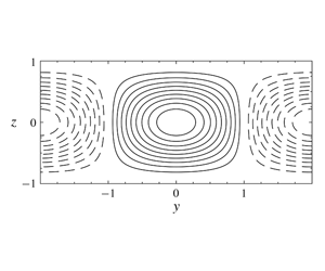
Figure 6. (a,b) First two singular response modes ($u_{1}$, $u_{2}$) of $G$; and first two singular forcing modes ($v_{1}$ and $v_{2}$) of $S$ for Couette flow (c,d) and Poiseuille flow (e,f). In each panel the singular modes are shown in physical space on the left (laminar velocity profiles only); and in Fourier space on the right (laminar and turbulent velocity profiles; lighter lines correspond to larger friction Reynolds numbers). In each plot the scaling is arbitrary.

The first two singular response modes ($u_{1}$ and $u_{2}$) of the Orr–Sommerfeld operator $G$ are shown in figure 6(a,b). (These are plotted in physical space, $u_{i}(y,z)$, on the left and in Fourier space, $u_{i}(k=\unicode[STIX]{x03C0}/2,z)$, on the right of each panel.) Recall that, for streamwise-constant fluctuations, the Orr–Sommerfeld operator is independent of the mean velocity profile. Therefore $u_{1}$ and $u_{2}$ remain the same across all of the velocity profiles that we consider (Couette and Poiseuille; laminar and turbulent). The first response mode, $u_{1}$, spans the entire channel height and is symmetric about the channel centre (reaching its peak response there). The second response mode, $u_{2}$, is anti-symmetric about the channel centre (where it is zero).

The first two singular forcing modes ($v_{1}$ and $v_{2}$) of the Squire operator $S$ for laminar Couette flow are shown in figure 6(c,d). (Again, these are plotted both in Fourier space and in physical space.) The first forcing mode $v_{1}$ is symmetric about the channel centre and is similar to $u_{1}$; and the second forcing mode $v_{2}$ is anti-symmetric about the channel centre and is similar to $u_{2}$. This similarity between the leading forcing modes of $G$ and the leading response modes of $S$ can be quantified by looking at the inner products $v_{1}^{\ast }u_{1}$ and $v_{2}^{\ast }u_{2}$. (This is equivalent to looking at the first two diagonal entries of $V_{S}^{\ast }U_{G}$.) These are $v_{1}^{\ast }u_{1}=0.985$ and $v_{2}^{\ast }u_{2}=0.971$. (The maximum possible value is 1 since $U_{G}$ and $V_{S}$ are each orthonormal.) These values are also summarized in table 3.

Table 3. Summary of the inner products $v_{i}^{\ast }u_{j}$ for $i,j=1,2$ (equivalent to looking at the first two diagonal entries of $V_{S}^{\ast }U_{G}$).

The story is quite different for laminar Poiseuille flow. The first two singular forcing modes ($v_{1}$ and $v_{2}$) of the Squire operator $S$ for laminar Poiseuille flow are shown in figure 6(e,f). The first forcing mode, $v_{1}$, is anti-symmetric about the channel centre; while the second forcing mode, $v_{2}$ is symmetric. The anti-symmetry of $v_{1}$ means that its inner product with $u_{1}$ (which is symmetric) is zero, $v_{1}^{\ast }u_{1}=0$. Thus the different symmetries of laminar Poiseuille flow mean that the leading forcing mode of the Squire operator is not excited by the leading response mode of the Orr–Sommerfeld operator. (The two modes are orthogonal.) In a similar way, the symmetry of $v_{2}$ means that its inner product with $u_{2}$ (which is anti-symmetric) is zero, $v_{2}^{\ast }u_{2}=0$. Thus for Poiseuille flow the important interactions are the second response mode with the first forcing mode ($v_{1}^{\ast }u_{2}=0.931$); and the first response mode with the second forcing mode ($v_{2}^{\ast }u_{1}=0.515$). This limits the forcing efficiency of laminar Poiseuille flow and is a consequence of its anti-symmetrical shear profile $U^{\prime }$.

Similar arguments apply when we replace the laminar velocity profiles of § 3 with the turbulent mean velocity profiles of § 4. In particular the first forcing mode $v_{1}$ of the Squire operator is symmetric for turbulent Couette flow and anti-symmetric for turbulent Poiseuille flow; and the second forcing mode $v_{2}$ is anti-symmetric for turbulent Couette flow and symmetric for turbulent Poiseuille flow. These first two forcing modes are shown in figure 6(c–f) for all Reynolds numbers considered alongside their laminar counterparts. (For brevity they are shown only in Fourier space.) Thus the symmetries observed in the leading forcing modes of $S$ for laminar Couette flow and laminar Poiseuille flow are retained by their turbulent counterparts. The most notable difference is that, for the turbulent mean velocity profiles, the leading forcing modes display peaks near the channel walls. These peaks occur for both Couette flow and Poiseuille flow and they move closer to the wall as Reynolds number increases. This is not surprising given the crucial role of the mean wall-normal shear for the Squire operator – and that this shear becomes increasingly concentrated at the wall with increasing Reynolds number. This in turn causes a reduction in the inner products considered earlier. For Couette flow the inner product $v_{1}^{\ast }u_{1}$ reduces from 0.985 (laminar) to 0.544 ($R_{\unicode[STIX]{x1D70F}}=986$); and the inner product $v_{2}^{\ast }u_{2}$ reduces from 0.971 (laminar) to 0.496 ($R_{\unicode[STIX]{x1D70F}}=986$). For Poiseuille flow the inner product $v_{2}^{\ast }u_{1}$ reduces from 0.515 (laminar) to 0.385 ($R_{\unicode[STIX]{x1D70F}}=950$); and the inner product $v_{1}^{\ast }u_{2}$ reduces from 0.931 (laminar) to 0.806 ($R_{\unicode[STIX]{x1D70F}}=950$). (These values are also summarized in table 3.) This indicates (for both flows) a reduction in the projection of the leading response modes of $G$ onto the leading forcing modes of $S$ and helps to explain the reduced efficiency $\unicode[STIX]{x1D6FC}$ for the turbulent mean velocity profiles observed in figures 4 and 5.

We finish this section by considering why laminar Couette flow displays almost perfect forcing efficiency, $\unicode[STIX]{x1D6FC}\approx 1$. This is explained by the fact that, for laminar Couette flow, the shear profile satisfies $U^{\prime }(z)=1$ everywhere. Thus the Squire operator becomes simply $S=(sI-\unicode[STIX]{x1D6E5})^{-1}$, the dynamics of which is similar to that of $(s\unicode[STIX]{x1D6E5}-\unicode[STIX]{x1D6E5}^{2})^{-1}$, which appears in the Orr–Sommerfeld operator $G(s)$ (see (2.4a)). It is then perhaps not surprising that the leading forcing modes of $S$ in figure 6(a,b) are so similar to the leading response modes of $G$ in figure 6(c,d). More generally (not shown) the $i\text{th}$ forcing mode of $S$ is similar to the $i\text{th}$ response mode of $G$ and thus the inner product $v_{i}^{\ast }u_{i}$ is close to unity.

6.1 Effect on the Orr–Sommerfeld operator $G$

We observed in § 2.3 that, for the kinematic viscosity, the Orr–Sommerfeld operator $G(s)$ is independent of the mean velocity profile and is therefore identical for Couette flow and Poiseuille flow. This is no longer true for the linear model (6.1) because the operator $G(s)$ now depends on the eddy-viscosity profile, which itself depends on the mean velocity profile. This ultimately means that we must now compare three linear operators: (i) $G$ using the kinematic viscosity (valid for both flows); (ii) $G$ for Couette flow with eddy viscosity; and (iii) $G$ for Poiseuille flow with eddy viscosity. For simplicity we do this comparison only for the largest friction Reynolds number available – for which we expect the influence of the eddy viscosity to be most significant. For Couette flow this is $R_{\unicode[STIX]{x1D70F}}=986$ and for Poiseuille flow it is $R_{\unicode[STIX]{x1D70F}}=950$.

Figure 7. (a) The infinity norm of the Orr–Sommerfeld operator, $\Vert G\Vert _{\infty }$; and (b,c) wall-normal variation of the (b) first and (c) second response modes of $G$. In each panel results are shown for the linear model with kinematic viscosity (2.2) (solid lines) and for the linear model with eddy viscosity (6.1) for Couette flow (dashed lines) and Poiseuille flow (dot–dashed lines). In (b,c) the scaling is arbitrary.

Figure 7 summarizes the influence of the eddy viscosity on the Orr–Sommerfeld operator $G(s)$. In panel (a) we plot the infinity norm, $\Vert G\Vert _{\infty }$ with spanwise wavenumber $k$ for the three operators. The three curves have each been normalized by their maximum value to aid comparison. We see that including an eddy viscosity reduces the spanwise wavenumber at which the peak response occurs: for the kinematic viscosity this peak occurs at $k_{max}=2.00$; with eddy viscosity the peak reduces to $k_{max}=1.44$ for Couette flow and to $k_{max}=1.47$ for Poiseuille flow. Therefore including an eddy viscosity in the linear operator does modify the behaviour of the Orr–Sommerfeld operator $G$. But this modification is relatively small and we ultimately draw the same conclusion as we did for the kinematic viscosity: that the Orr–Sommerfeld operator has a preferred spanwise wavenumber; and that this is in the region of $k\approx 1{-}2$. In panels (b,c) we plot the first two singular response modes of $G$ for the three cases. We see that including an eddy viscosity in the linear operator modifies these response modes. But again, this modification is relatively small and we ultimately draw the same conclusions as we did for the kinematic viscosity: that both response modes are channel-wide; that the first response mode is symmetric about the channel centre; and that the second response mode is anti-symmetric about the channel centre.

6.2 Effect on $k_{max}$ and $\unicode[STIX]{x1D6FC}_{max}$

We now consider the effect of the eddy viscosity on the overall operator $F(s)$. In particular, we will look at the influence on the spanwise wavenumber at which $\Vert F\Vert _{\infty }$ attains its maximum ($k_{max}$); and the efficiency attained at this maximum ($\unicode[STIX]{x1D6FC}_{max}$). In other words we repeat here the results of figure 5 using the linear model (6.1) so that an eddy viscosity is included in the overall operator $F(s)$.

Figure 8. Summary of key results for the linear model with eddy viscosity (6.1) as a function of friction Reynolds number $R_{\unicode[STIX]{x1D70F}}$: (a) spanwise wavenumber, $k_{max}$, at which $\Vert F\Vert _{\infty }$ attains its maximum; and (b) the efficiency, $\unicode[STIX]{x1D6FC}_{max}$, attained at this maximum. Results are shown for turbulent Couette flow (▴) and turbulent Poiseuille flow (▪). Results from figure 5 for the linear model with kinematic viscosity (2.2) are also shown (▵, ▫).

The results are plotted in figure 8. We plot in panel (a) the spanwise wavenumber $k_{max}$ at which $\Vert F\Vert _{\infty }$ attains its maximum; and in panel (b) the efficiency $\unicode[STIX]{x1D6FC}_{max}$ attained at this maximum. We also plot these same quantities for the laminar velocity profiles (dashed lines) and for the turbulent velocity profiles without eddy viscosity (open symbols), which were also plotted in figure 5. In panel (a) we see that, for both flows, the effect of including an eddy viscosity is to reduce $k_{max}$. For Poiseuille flow the reduction in $k_{max}$ is at most 25 % (from $k_{max}=1.60$ to $k_{max}=1.2$ at $R_{\unicode[STIX]{x1D70F}}=950$). For Couette flow the reduction in $k_{max}$ is much larger: the largest reduction is 50 % (from $k_{max}=1.2$ to $k_{max}=0.6$ at $R_{\unicode[STIX]{x1D70F}}=986$). This is broadly consistent with the results obtained by Hwang & Cossu (Reference Hwang and Cossu2010a). Using the linearized Navier–Stokes equations for Couette flow at a lower friction Reynolds number of $R_{\unicode[STIX]{x1D70F}}=52$, they found a preferred spanwise wavenumber for harmonic forcing (the infinity norm) of $k_{max}=0.82$ (which corresponds to a spanwise wavelength of $\unicode[STIX]{x1D706}_{max}=7.7h$). These results are all in quite poor agreement with DNS and experiments, where the spanwise dimensions of the channel-wide streamwise streaks are in the approximate range of $\unicode[STIX]{x1D706}\approx 4{-}5h$ ($k=1.26{-}1.57$) (Pirozzoli et al. Reference Pirozzoli, Bernardini and Orlandi2014). It seems, then, that the eddy viscosity is less appropriate for Couette flow – at least for streamwise-constant modes – and this is likely in part for the reasons discussed earlier in § 2.2.

In panel (b) we see that, for both flows, including an eddy viscosity significantly reduces $\unicode[STIX]{x1D6FC}_{max}$. To give some indication, the average value of $\unicode[STIX]{x1D6FC}_{max}$ across all turbulent Reynolds numbers reduces from 0.24 to 0.09 for Poiseuille flow; and from 0.60 to 0.19 for Couette flow. Despite this, it is important to stress that the efficiency achieved by Couette flow is still in every case larger than that for Poiseuille flow by a factor of approximately 2. Thus although the efficiency of both flows is reduced by the inclusion of an eddy viscosity, the efficiencies of the two flows relative to each other remains approximately the same. (Specifically, at the highest Reynolds numbers available, the ratio of efficiencies is 2.15 when using the kinematic viscosity and is 2.09 when using the eddy viscosity.) We can therefore still conclude that Couette flow is significantly more efficient than Poiseuille flow, even if the efficiency of both flows is reduced.