1. Vortex defects in quantum fluids

In recent years experimental realization of Bose–Einstein condensates (Andrews et al. Reference Andrews, Townsend, Miesner, Durfee, Kurn and Ketterle1997; Cornell & Wieman Reference Cornell and Wieman1998) as new states of matter, and laboratory production of vortex defects (Matthews et al. Reference Matthews, Anderson, Haljan, Hall, Wieman and Cornell1999), have stimulated a renovated interest in theoretical, numerical and experimental work in condensed matter physics. The hydrodynamic interpretation of the governing equations – rooted in the original work of Madelung (Reference Madelung1926) – coupled with the extraordinary recent progress in direct numerical simulation of fluid flows, has given further impetus (Wyatt Reference Wyatt2005). Here, considering a vortex defect subject to superposed phase twist, we derive the Gross–Pitaevskii equation in the presence of twist, determine the twist state energy, derive the correct continuity and momentum equation and work out the complete set of hydrodynamic equations governing twist evolution and vortex dynamics. With the help of this new set of equations we can investigate details of the first stage of vortex evolution governed by twist energy relaxation and possible production of new defects.

A condensate is a highly diluted gas of bosons that at ultra-cold temperatures can be modelled by the Gross–Pitaevskii equation (GPE) (Pitaevskii Reference Pitaevskii1961; Gross Reference Gross1961). This is a mean-field equation that in non-dimensional form is given by

(1.1)\begin{equation} \frac{\partial \psi}{\partial t} = \frac{\mathrm{i}}2 {{\nabla}^2} \psi + \frac{\mathrm{i}}{2} (1 - |\psi|^2 )\psi\quad \textrm{(GPE)}\end{equation}

for the single, complex wave function $\psi =\psi ({\boldsymbol {x}}, t)$, where ${\boldsymbol {x}}$ is the 3-space variable and $t$ time. For simplicity, we assume an unbounded domain and background density $\rho =|\psi |^2 \to 1$ as $|{\boldsymbol {x}}| \to \infty$. In this context, phase defects emerge as nodal lines of the wave function $\psi$. By using the Madelung transformation $\psi = \sqrt \rho \, \mathrm {exp}(\mathrm {i} \chi )$, where $\chi$ is the phase of $\psi$, the real and imaginary parts of (1.1) give rise to the continuity and momentum equation of a fluid-like medium of density $\rho$ and velocity ${\boldsymbol {u}}=\boldsymbol {\nabla } \chi$. This allows a macroscopic interpretation of the condensate in terms of standard hydrodynamics (Barenghi & Parker Reference Barenghi and Parker2016). In the presence of phase twist standard theory needs correction, and this is what we intend to address here.

In the context of quantum fluids a defect ${\mathcal {L}}$ is a zero-density line of quantized circulation given (per unit of mass) by $\varGamma =2{\rm \pi} n$ ($n=1,2,\ldots$). Quantization of circulation arises naturally from line integration of ${\boldsymbol {u}}=\boldsymbol {\nabla } \chi$ over a simple loop encircling ${\mathcal {L}}$ and from the multi-valuedness of $\chi$. The vortex is thus a true, topological defect embedded in a three-dimensional, irrotational fluid medium (since $\boldsymbol {\nabla } \times \boldsymbol {u}=\boldsymbol {\nabla } \times \boldsymbol {\nabla } \chi =0$), whose charge is given by vortex circulation.

The novelty is to consider a vortex defect in the presence of twist. As mentioned above, the emergence of a defect demands a correction of the standard momentum equation that governs an irrotational fluid; moreover, the actual presence of phase twist also has implications for stability and vortex dynamics. Recent numerical simulations (Zuccher & Ricca Reference Zuccher and Ricca2018) and theoretical work (Foresti & Ricca Reference Foresti and Ricca2019) demonstrate that new defects can be produced by pure injection of phase twist on existing defects. As pointed out by Foresti & Ricca (Reference Foresti and Ricca2019), this observation has interesting potential applications in science and technology. In order to understand and exploit details associated with twist energy and vortex dynamics we derive the correct set of governing equations for defects in the presence of twist. Since the ambient domain is multiply connected we must consider appropriate correction to the governing equations due to a multi-valued potential, and this is done by applying the defect gauge theory developed by Kleinert (Reference Kleinert2008).

The material is presented as follows: in § 2 we derive the modified Gross–Pitaevskii equation (mGPE) for a twist state, and in § 3 we show that this state corresponds to an excitation of the fundamental energy level. We prove that the Hamiltonian is non-Hermitian and show how twist may influence stability. In § 3.1 we consider as explicit example, the case of a vortex ring subject to uniform axial twist. In § 4 we introduce the standard hydrodynamic formulation of GPE, determine the continuity equation when twist is present and derive the correct momentum equation of the system when a vortex defect is present. Finally, in § 5 we consider twist kinematics and vortex dynamics and determine the complete set of hydrodynamic equations governing the evolution of the defect. Conclusions are drawn in § 6.

2. Modified Gross–Pitaevskii equation for twisted state

Let us consider the superposition of phase twist $\theta _{tw}$ on an existing defect, which is identified by a smooth, closed space curve ${\mathcal {L}}$ of vector position ${\boldsymbol {X}}={\boldsymbol {X}}(s)$, $s$ arc-length and total length $L$. As anticipated, ${\mathcal {L}}$ is a nodal line of the wavefunction $\psi$, so it can be interpreted as the locus of intersection of a fan of isosurfaces $\bar \chi$ (surfaces of constant phase) that foliate the entire space. In this context, twist is given by the longitudinal rotation of the phase of the isosurfaces hinged on ${\mathcal {L}}$. To define twist adequately we refer to the mathematical ribbon $R=R({\mathcal {L}},{\mathcal {L}}^*)$ identified by the portion of $\bar \chi$ bounded by ${\mathcal {L}}$ (the ribbon baseline edge) and the curve ${\mathcal {L}}^*$ on $\bar \chi$ given by ${\mathcal {L}}^*: {\boldsymbol {X}}+\epsilon {\boldsymbol {\hat U}}$, where $\epsilon =\,$constant denotes ribbon width (that can be taken of the order of the defect healing length) and ${\boldsymbol {\hat U}}={\boldsymbol {\hat U}}(s)$ the ribbon spanwise unit vector normal to ${\mathcal {L}}$. Incremental twist is defined by

(2.1)\begin{equation} \theta_{tw}(s) = \int_0^s \left({\boldsymbol{\hat U}}\times\frac{\textrm{d}{\boldsymbol{\hat U}}}{\textrm{d}\bar s} \right)\boldsymbol{\cdot}{\boldsymbol{\hat T}}\,\textrm{d}\bar s, \end{equation}

where ${\boldsymbol {\hat T}}={\boldsymbol {\hat T}}(s)\equiv \textrm {d}\,{\boldsymbol {X}}/\textrm {d} s$ is the standard unit tangent to ${\mathcal {L}}$ and $\bar s$ a dummy variable. Total twist is given by the cumulative rotation of the ribbon spanwise unit vector ${\boldsymbol {\hat U}}$ from some origin $s=0$ to $L$. Here, for simplicity, we assume ${\mathcal {L}}$ to be closed and inextensible, with total twist number given by $Tw=(2{\rm \pi} )^{-1}\theta _{tw}(L)$. In the presence of stretching the definition can be easily adapted to include a functional dependence of $s$ on time.

In the following we shall consider the space–time evolution of ${\mathcal {L}}$, so that ${\boldsymbol {X}}={\boldsymbol {X}}(s,t)$ and $\theta _{tw}=\theta _{tw}(s,t)$ on ${\mathcal {L}}$, so that, in general, $\theta _{tw} = \theta _{tw}({\boldsymbol {x}}, t)$. Several experimental techniques to inject twist locally and to get it spread in the bulk of the condensate can be used, including the method proposed by the present authors (see Foresti & Ricca Reference Foresti and Ricca2019, § V, B) based on the exploitation of the Berry phase (Leanhardt et al. Reference Leanhardt, Görlitz, Chikkatur, Kielpinski, Shin, Pritchard and Ketterle2002). Twist thus produced on the defect is then instantly distributed in the condensate because of the contextual nature of the governing wave function that characterizes the system (Pitaevskii & Stringari Reference Pitaevskii and Stringari2016).

If $\psi _0$ denotes the fundamental state, the superposed twist state $\psi _1$ is defined by the following transformation:

(2.2)\begin{equation} \psi_0 \rightarrow \psi_1 = \mathrm{e}^{\mathrm{i} \theta_{tw}({\boldsymbol{x}}, t)}\psi_0. \end{equation}

Since the GPE is not invariant under local phase transformation, in the twist superposition transient $\psi _1$ does not evolve under the same GPE. Let us determine the modified equation. From (2.2) we have

(2.3)\begin{equation} \partial_t{\psi_1} = (\partial_t\, \mathrm{e}^{\mathrm{i}\theta_{tw}})\psi_0 + (\partial_t\psi_0)\,\mathrm{e}^{\mathrm{i}\theta_{tw}}. \end{equation}

Substituting the GPE (1.1) into the right-hand side term above and re-arranging terms, we have

(2.4)\begin{equation} \partial_t{\psi_1}=\mathrm{i}(\partial_t\theta_{tw})\psi_1 + \frac{\mathrm{i}}{2}({{\nabla}^2} \psi_0)\,\mathrm{e}^{\mathrm{i}\theta_{tw}} + \frac{\mathrm{i}}{2}(1 - |\psi_1|^2) \psi_1,\end{equation}

where we have taken $|\psi _0| = |\psi _1|$.

Using the vector identity $\mathrm {e}^{\mathrm {i}\theta _{tw}}{{\nabla }^2} \psi _0 = \boldsymbol {\nabla } \boldsymbol {\cdot }(\mathrm {e}^{\mathrm {i}\theta _{tw}}\boldsymbol {\nabla } \psi _0) -(\boldsymbol {\nabla } \mathrm {e}^{\mathrm {i}\theta _{tw}})\boldsymbol {\cdot }\boldsymbol {\nabla } \psi _0$ and substituting (2.2), after some straightforward algebra we have

(2.5)\begin{equation} \partial_t\psi_1 = \mathrm{i}(\partial_t\theta_{tw})\psi_1 + \frac{\mathrm{i}}{2} (\boldsymbol{\nabla} - \mathrm{i}\boldsymbol{\nabla} \theta_{tw})^2\psi_1 +\frac{1}{2}\boldsymbol{\nabla} \theta_{tw}\boldsymbol{\cdot}\boldsymbol{\nabla} \psi_1 + \frac{\mathrm{i}}{2}(1 - |\psi_1|^2) \psi_1. \end{equation}

The correct evolution equation is a modified form of the standard Gross–Pitaevskii equation, given by

(2.6)\begin{equation} \partial_t\psi_1 =\frac{\mathrm{i}}{2} \boldsymbol{\tilde{\nabla}}^2\psi_1 + \frac{\mathrm{i}}{2}(1 - |\psi_1|^2) \psi_1 + \mathrm{i}(\partial_t\theta_{tw})\psi_1 + \frac{1}{2}\boldsymbol{\nabla} \theta_{tw}\boldsymbol{\cdot}\boldsymbol{\nabla} \psi_1 \quad\textrm{(mGPE)},\end{equation}

where $\boldsymbol {\tilde {\nabla }} = \boldsymbol {\nabla } - \mathrm {i}\boldsymbol {\nabla } \theta _{tw}$; the mGPE is still a Gross–Pitaevskii type of equation, with an extra interaction term given by phase twist and a flux term proportional to the gradient of $\theta _{tw}$ along ${\mathcal {L}}$ (for explicit computation of this flux and its interpretation in terms of axial fluid flow see again Foresti & Ricca (Reference Foresti and Ricca2019), and § 5 below).

3. Hamiltonian and energy

Before considering the actual vortex dynamics, few considerations about the Hamiltonian and energy of the twisted state are in order. The Hamiltonian (see, for instance, Barenghi & Parker (Reference Barenghi and Parker2016, p. 111)) associated with the mGPE above is given by

(3.1)\begin{equation} H_{tw} = \tfrac{1}{2} \, {\boldsymbol{\tilde{p}}}^2 - \tfrac{1}{2}(1 - |\psi_1|^2) - V_{tw}, \end{equation}

where ${\boldsymbol {\tilde {p}}}= {\boldsymbol {p}} - \boldsymbol {\nabla } \theta _{tw}$ is the canonical momentum of the twisted state, ${\boldsymbol {p}} = -\mathrm {i}\boldsymbol {\nabla }$ the momentum operator and $V_{tw}= \partial _t\theta _{tw} -(1/2)\boldsymbol {\nabla } \theta _{tw}\boldsymbol {\cdot }{\boldsymbol {p}}$ the twist potential. We have

Proof. The quadratic terms of ${\boldsymbol {\tilde {p}}}^2$ are Hermitian since both ${\boldsymbol {p}}$ and $\boldsymbol {\nabla } \theta _{tw}$ (proportional to the identity, and function of ${\boldsymbol {x}}$) are individually Hermitian; the self-interaction terms are also Hermitian (with pre-factor $(1 - |\psi _1|^2)$, a real number); the remaining part, however, is not Hermitian

(3.2)\begin{gather} (\boldsymbol{\nabla} \theta_{tw}\boldsymbol{\cdot}{\boldsymbol{p}})^\dagger= {\boldsymbol{p}}^\dagger\boldsymbol{\cdot}\boldsymbol{\nabla} \theta_{tw}^\dagger = {\boldsymbol{p}}\boldsymbol{\cdot}\boldsymbol{\nabla} \theta_{tw}; \end{gather}

(3.3)\begin{gather}(\boldsymbol{\nabla} \theta_{tw}\boldsymbol{\cdot}{\boldsymbol{p}})^\dagger\psi_1 = (\,{\boldsymbol{p}}\boldsymbol{\cdot}\boldsymbol{\nabla} \theta_{tw})\psi_1 = -\mathrm{i} {{\nabla}^2} \theta_{tw}\,\psi_1; \end{gather}

(3.4)\begin{gather}(\boldsymbol{\nabla} \theta_{tw}\boldsymbol{\cdot}{\boldsymbol{p}}) \psi_1 =-\mathrm{i} \boldsymbol{\nabla} \theta_{tw}\boldsymbol{\cdot}\boldsymbol{\nabla} \psi_1\neq (\boldsymbol{\nabla} \theta_{tw}\boldsymbol{\cdot}{\boldsymbol{p}})^\dagger\psi_1 . \end{gather}

Hence $H_{tw}^\dagger \neq H_{tw}$.

Properties of non-Hermitian Hamiltonians have been widely investigated in both classical and quantum contexts (Bender Reference Bender2007; El-Ganainy et al. Reference El-Ganainy, Makris, Khajavikhan, Musslimani, Rotter and Christodoulides2018), mainly when physical systems manifest loss and gain of energy. The implications for the twisted state become clear when we compute the energy expectation value given by $E_{tw}=\langle \psi _1|H|\psi _1\rangle /\langle \psi _1|\psi _1\rangle$ (taking care of the total number of particles present). This is given by

(3.5)\begin{align} E_{tw}= \int \left[\left(-\partial_t\theta_{tw}|\psi_1|^2 +\frac{\mathrm{i}}{2}\psi_1^*\boldsymbol{\nabla} \theta_{tw}\boldsymbol{\cdot}\boldsymbol{\nabla} \psi_1\right) +\frac{1}{2} |\boldsymbol{\tilde{\nabla}}\psi_1|^2 -\frac{1}{2} |\psi_1|^2 + \frac{1}{4}|\psi_1|^4\right] \, \textrm{d} V ,\end{align}

where $\textrm {d} V$ denotes the volume element of the condensate. We see that the expectation value of $V_{tw}$ (first term in brackets) has, in this case, an imaginary part. Upon application of the Madelung transform $\psi _1 = \sqrt \rho \, \mathrm {exp}(\mathrm {i} \chi _1)$, we have

(3.6)\begin{equation} \left. \begin{array}{c@{}} \mathrm{Re}\langle\psi_1|V_{tw}|\psi_1\rangle= -\partial_t\theta_{tw} - \frac{1}{2}\rho\boldsymbol{\nabla} \theta_{tw}\boldsymbol{\cdot}\boldsymbol{\nabla} \chi_1, \\ \mathrm{Im} \langle\psi_1|V_{tw}|\psi_1\rangle = \frac{1}{4}\boldsymbol{\nabla} \theta_{tw}\boldsymbol{\cdot}\boldsymbol{\nabla} \rho. \end{array} \right\} \end{equation}

It is the imaginary term above that makes the Hamiltonian non-Hermitian; moreover, $E_{tw}$ depends on time through $\partial _t\theta _{tw}$. The non-Hermiticity of $H_{tw}$ provides an alternative proof that a twisted state in isolation is indeed unstable. Confirmation of this comes from linear perturbation of the mGPE: the perturbed state is given by

(3.7)\begin{equation} \tilde{\psi} = \psi_1 + \psi_{1p}=\psi_1+|\psi_{1p}|\,\mathrm{e}^{\mathrm{i}(\boldsymbol{k}\boldsymbol{\cdot}{\boldsymbol{x}} - \nu\,t)}, \quad |\psi_{1p}|\ll|\psi_1|, \end{equation}

where $\psi _1$ is the unperturbed state and $|\psi _{1p}|= \textrm {constant}$, $\boldsymbol {k}$ wave vector, $\nu$ perturbation frequency. By substituting $\tilde {\psi }$ into (2.6) and retaining only first-order terms, we obtain the dispersion relation

(3.8)\begin{equation} \nu = \tfrac{1}{2}[(|\boldsymbol{k}|^2 - 2\boldsymbol{\nabla} \theta_{tw}\boldsymbol{\cdot}\boldsymbol{k} + |\boldsymbol{\nabla} \theta_{tw}|^2-1-\partial_t\theta_{tw})+\mathrm{i}\nabla^2\theta_{tw} ] .\end{equation}

Considering the imaginary part of the frequency, we can state the following:

1. (a) $\nabla ^2\theta _{tw} < 0$: we have damped oscillations with $\tilde {\psi } \rightarrow \psi _0$ as $t \rightarrow \infty$;

2. (b) $\nabla ^2\theta _{tw} = 0$: oscillatory terms survive and the system is stable;

3. (c) $\nabla ^2\theta _{tw} > 0$: we have instability with $|\psi |\rightarrow \infty$ as $t \rightarrow \infty$.

Non-Hermiticity of the Hamiltonian is given by $\boldsymbol {\nabla } \theta _{tw}\boldsymbol {\cdot }\boldsymbol {\nabla } \rho \neq 0$. In summary we have:

1. (i) if $\boldsymbol {\nabla } \theta _{tw}\boldsymbol {\cdot }\boldsymbol {\nabla } \rho =0$ and ${{\nabla }^2} \theta _{tw}\le 0$, then $H_{tw}$ is Hermitian and the system is linearly stable under small perturbations;

2. (ii) if $\boldsymbol {\nabla } \theta _{tw}\boldsymbol {\cdot }\boldsymbol {\nabla } \rho \neq 0$ and ${{\nabla }^2} \theta _{tw}\le 0$, then $H_{tw}$ is not Hermitian with (probability) density not conserved: there is phase twist diffusion due to the Laplacian and the system is still linearly stable under small perturbations;

3. (iii) if $\boldsymbol {\nabla } \theta _{tw}\boldsymbol {\cdot }\boldsymbol {\nabla } \rho = 0$ and ${{\nabla }^2} \theta _{tw}>0$, then $H_{tw}$ is Hermitian, and the system is linearly unstable under small perturbations;

4. (iv) if $\boldsymbol {\nabla } \theta _{tw}\boldsymbol {\cdot }\boldsymbol {\nabla } \rho \neq 0$ and ${{\nabla }^2} \theta _{tw}> 0$, then $H_{tw}$ is non-Hermitian and the system is linearly unstable, with phase diffusion due to the flux of $\rho \boldsymbol {\nabla } \theta _{tw}$ along ${\mathcal {L}}$.

Note that the Hermiticity of the Hamiltonian can also be attained by allowing the potential twist $V_{tw}$ to move freely, as if it were caused by a second topological defect interacting in the system. As mentioned by Gong et al. (Reference Gong, Ashida, Kawabata, Takasan, Higashikawa and Ueda2018), pointing out the possible role of topology in relation to stability aspects, in the vortex ring case of figure 1 we have an explicit demonstration that twist instability is indeed what triggers topological changes and the corresponding production of a new defect. The process can be seen as an energy relaxation mechanism in response to twist superposition.

Figure 1. (a) Initial condition given by a planar vortex ring visualized by the iso-density tubular surface $\rho =0.1$. The arrow indicates the vorticity direction. (b) Twist $Tw=1$ is superposed (say at $t=0$) by prescribing a full rotation of the isophase $\bar \chi$ (as described in detail in § 3.1), shown by the phase contour in the $(y,z)$-plane. (c) The presence of twist induces the instantaneous production of a new, central defect, here shown at a later time (adapted from Zuccher & Ricca Reference Zuccher and Ricca2018). Note the corrugation of the iso-density surface that reflects perturbation of the density profile.

3.1. Vortex ring case

The simple case of uniform phase twist superposed on a vortex ring ${\mathcal {L}}_0$ of radius $R_0$ provides an explicit example. In the zero-twist case the vortex propagates steadily in the medium without change of shape (see figure 1a), with conserved energy $E_0=E(\theta _{tw}=0)$ (Barenghi & Parker Reference Barenghi and Parker2016). Suppose now that at some time (say $t=0$) we superpose instantly uniform twist $\theta _{tw}=w\alpha$, where $w$ denotes the winding number of ${\boldsymbol {\hat U}}$ around ${\mathcal {L}}_0$ and $\alpha$ is the azimuth angle. In cylindrical coordinates $(r,\alpha ,z)$ centred on the ring, we have

(3.9a,b)\begin{equation} \boldsymbol{\nabla} \theta_{tw}=\frac{w}{R_0}{\boldsymbol{\hat e}_\alpha}, \quad \partial_t\theta_{tw} = \boldsymbol{\nabla} \theta_{tw}\boldsymbol{\cdot}\boldsymbol{\nabla} \psi_1 = 0, \end{equation}

where ${\boldsymbol {\hat e}_\alpha }$ is the azimuth unit vector. The new energy state is now given by

(3.10)\begin{equation} E_{tw}= \int \left(\frac{1}{2} \left|\boldsymbol{\nabla} \psi_1-\mathrm{i} w \frac{w}{R_0}{\boldsymbol{\hat e}_\alpha}\psi_1\right|^2 -\frac{1}{2} |\psi_1|^2 + \frac{1}{4}|\psi_1|^4\right) \, \textrm{d} V .\end{equation}

Evidently, we have

(3.11)\begin{equation} E_{tw} = E_0+ \frac{1}{2}\left(\frac{w}{R}\right)^2|\psi_1|^2 \geq E_0, \end{equation}

where $E_{tw}$ is quadratic in $w$, and $E_{tw} = E_0$ if and only if $w = 0$. As Foresti & Ricca (Reference Foresti and Ricca2019) demonstrated, topological and dynamical arguments show that superposition of twist generates in this case instantaneous production of a new, central defect, as shown in figure 1(c).

4. Hydrodynamic equations in the presence of twist

It is well known (see again Barenghi & Parker Reference Barenghi and Parker2016) that by applying the Madelung transformation to (1.1) the real and imaginary parts of the GPE give rise to the momentum and continuity equation of a fluid-like medium. By following the same procedure, substitution of $\psi _1 = \sqrt \rho \, \mathrm {exp}(\mathrm {i} \chi _1)$ into the mGPE gives rise to the set of equations

(4.1)\begin{gather} \partial_t\rho + \boldsymbol{\nabla} \boldsymbol{\cdot}(\rho{\boldsymbol{u}}) = \boldsymbol{\nabla} \boldsymbol{\cdot}(\rho\boldsymbol{\nabla} \theta_{tw}), \end{gather}

(4.2)\begin{gather}\partial_t\chi_1 = \tfrac{1}{2}[1-\rho-({\boldsymbol{u}} - \boldsymbol{\nabla} \theta_{tw})^2] + Q + \partial_t\theta_{tw}, \end{gather}

where $Q = {{\nabla }^2} \sqrt {\rho }/(2\sqrt {\rho })$ is the so-called quantum potential. Equation (4.1) is the new continuity equation, where change in (probability) density is now balanced by diffusion of twist; the gradient of (4.2) generates the momentum equation in hydrodynamic form. When a defect is present this equation must be modified to take into account the multi-valued phase. To implement this correction we follow the defect gauge theory developed by Kleinert (Reference Kleinert2008) and applied by dos Santos (Reference dos Santos2016) to multi-valued potentials. Indeed, in analogy with Helmholtz's decomposition of classical fluid mechanics, we have

(4.3)\begin{equation} {\boldsymbol{u}}={\boldsymbol{u}}_{I}+{\boldsymbol{u}}_{R}=\boldsymbol{\nabla} \chi_1+{\boldsymbol{A}}=\boldsymbol{\nabla} \chi_1+A\boldsymbol{\delta}_{\bar\chi_1}({\boldsymbol{x}}),\end{equation}

where ${\boldsymbol {u}}_{I}$ is irrotational and ${\boldsymbol {u}}_{R}\equiv {\boldsymbol {A}}$ denotes the rotational contribution given by the vector potential ${\boldsymbol {A}}=A\boldsymbol {\delta }_{\bar \chi _1}({\boldsymbol {x}})$ due to the singular distribution of vorticity; ${\boldsymbol {A}}$ is directed along the normal to the cut-isophase surface $\bar \chi _1$ through which we have the phase jump (see figure 2b,c); we take $A=$ constant and $\boldsymbol {\delta }_{\bar \chi _1}({\boldsymbol {x}})=\int _{\bar \chi _1}\delta ^{(3)}({\boldsymbol {x}}-{\boldsymbol {x}}')\,\textrm {d}{\boldsymbol {x}}'$, $\forall {\boldsymbol {x}}'\in \bar \chi _1$ (see Kleinert Reference Kleinert2008).

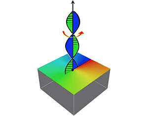
Figure 2. Straight defect along the $z$ axis: (a) density profile around the nodal line $\rho =0$; (b) case of zero phase twist, with phase jump across the positive half-plane $(x,z)$ (evidenced by the blue half-plane online); (c) case of uniform phase twist with winding number $w$.

Following dos Santos (Reference dos Santos2016) it is convenient to write ${\boldsymbol {A}}$ in terms of the 4 components $\{A_\mu \}$, with $\mu =1,2,3$ to denote space and $\mu =0$ time. In analogy with the electric/magnetic decomposition associated with the Faraday tensor, we write

(4.4)\begin{equation} E_\mu= \partial_{0}A_{\mu} - \partial_{\mu}A_{0} . \end{equation}

Consider now the four-dimensional velocity field, that in components is given by

(4.5)\begin{equation} u_{\mu}= \frac{{\psi_1}^*\partial_{\mu}\psi_1 - {\psi_1}\partial_{\mu}\psi_1^*}{2i\psi_1^*\psi_1},\end{equation}

($\psi _1^*$ complex conjugate), where now $u_0 \equiv \partial _t\chi _1+A_0$. In order to determine the new time derivative of the velocity when the defect is present, we note that

(4.6)\begin{equation} \partial_{\mu}u_0 = \partial_{\mu}(\partial_0\chi_1 + A_0) = \partial_0 (\partial_{\mu}\chi_1+ A_\mu) + (\partial_{\mu}A_0 - \partial_{0}A_\mu); \end{equation}

substituting (4.4) into the last bracket of the equation above, we have $\boldsymbol {\nabla } u_0= \partial _t {\boldsymbol {u}} - {\boldsymbol {E}}$, i.e.

(4.7)\begin{equation} \partial_t {\boldsymbol{u}}=\boldsymbol{\nabla} u_0+{\boldsymbol{E}},\end{equation}

that gives the correct momentum equation. Since ${\boldsymbol {u}}=\boldsymbol {\nabla } \chi _1+{\boldsymbol {A}}$, to take account of the cut effects on the time component of ${\boldsymbol {u}}$ we must replace the term $\partial _t\chi _1$ on the left-hand side of (4.2) with $\partial _t\chi _1+A_0$, i.e. $\partial _t\chi _1 \to \partial _t\chi _1+A_0$, so that (4.2) becomes

(4.8)\begin{equation} u_0=\partial_t\chi_1+A_0 = \frac{1}{2}[1-\rho-({\boldsymbol{u}} - \boldsymbol{\nabla} \theta_{tw})^2] + Q + \partial_t\theta_{tw}.\end{equation}

The value of ${\boldsymbol {E}}$ can then be worked out considering the jump of the vector potential ${\boldsymbol {A}}$ through the cut-isophase surface $\bar \chi _1$. Since defect dynamics is independent of the cut isosurface, we can always choose the cut (where ${\boldsymbol {A}}$ is defined) such that $\bar \chi _1=0$; for

(4.9)\begin{equation} \frac{\mathrm{Im}(\psi_1)}{\mathrm{Re}(\psi_1)}=\tan\chi_1=\tan0=0. \end{equation}

Hence, $\mathrm {Im}(\psi _1)=0$ for all $\mathrm {Re}(\psi _1)>0$ (see again figure 2b,c). This means that $\partial _\mu \bar \chi _1$ must have a discontinuity given by $-2{\rm \pi} \varTheta [\textrm {Re}(\psi _1)]\,\partial _\mu \varTheta [\textrm {Im}(\psi _1)]$ (dos Santos Reference dos Santos2016), so that the jump in the potential ${\boldsymbol {A}}=A\boldsymbol {\delta }_{\bar \chi _1}({\boldsymbol {x}})$ is given by

(4.10)\begin{equation} A_\mu=2{\rm \pi} \varTheta[\textrm{Re}(\psi_1)]\,\partial_\mu\varTheta[\textrm{Im}(\psi_1)],\end{equation}

where $\varTheta [\cdot ]$ is Heaviside's function (for this derivation consider the jump of $\boldsymbol {\delta }_{\bar \chi _1}({\boldsymbol {x}})$ across the cut in cylindrical polar coordinates; see dos Santos (Reference dos Santos2016, p. 30)). Thus, from (4.4) we have

(4.11)\begin{equation} E_i= 4{\delta}(\rho)[\partial_0(\textrm{Re}(\psi_1))\,\partial_i(\textrm{Im}(\psi_1)) -\partial_i(\textrm{Re}(\psi_1))\,\partial_0(\textrm{Im}(\psi_1))],\end{equation}

and after some algebra we have (dos Santos Reference dos Santos2016, (33))

(4.12)\begin{equation} {\boldsymbol{E}}= -2{\delta}(\rho) [\boldsymbol{\nabla} \boldsymbol{\cdot}(\rho{\boldsymbol{u}}-\rho\boldsymbol{\nabla} \theta_{tw})\,{\boldsymbol{u}} + u_0\boldsymbol{\nabla} \rho].\end{equation}

By substituting (4.12) into (4.7) we have the correct momentum equation, given by

(4.13)\begin{equation} \partial_t{\boldsymbol{u}} = \boldsymbol{\nabla} u_0- 2{\delta}(\rho)[\boldsymbol{\nabla} \boldsymbol{\cdot}(\rho{\boldsymbol{u}}-\rho\boldsymbol{\nabla} \theta_{tw})\,{\boldsymbol{u}} + u_0\boldsymbol{\nabla} \rho]. \end{equation}

Note the presence of the $\delta$-function on the right-hand side of the equation above, that justifies the correction to the standard momentum (4.2) due to the presence of the defect at $\rho =0$.

5. Twist kinematics and vortex dynamics

First let us consider twist kinematics when ${\mathcal {L}}$ evolves in time. For this we consider the standard intrinsic reference frame on ${\mathcal {L}}$ given by the Frenet triad $\{{\boldsymbol {\hat T}},{\boldsymbol {\hat N}},{\boldsymbol {\hat B}}\}$, where ${\boldsymbol {\hat N}}$ and ${\boldsymbol {\hat B}}$ denote principal unit normal and binormal vectors to ${\mathcal {L}}$, respectively. The time evolution of $\theta _{tw}$ is given by two contributions: one, referred to as the ‘dynamical phase’ (Hannay Reference Hannay1998), is due to the Lagrangian rotation of the ribbon unit vector ${\boldsymbol {\hat U}}$ around ${\mathcal {L}}$; the other, referred to as the ‘geometric phase’, is due to the evolution of ${\boldsymbol {X}}$ (hence ${\boldsymbol {\hat T}}$) in space. The evolution of twist in moving filaments (or ribbons) is derived by Klapper & Tabor (Reference Klapper and Tabor1994) by adding together these two contributions; this is given by

(5.1)\begin{equation} \partial_t\theta_{tw} = \int_0^s[\boldsymbol{\nabla} \chi_1\boldsymbol{\cdot}{\boldsymbol{\hat T}} + c\,(\partial_t{\boldsymbol{\hat T}})_B]\, \textrm{d} \bar s,\end{equation}

where $\boldsymbol {\nabla } \chi _1\boldsymbol {\cdot }{\boldsymbol {\hat T}}$ can be interpreted as a hydrodynamic axial flow that generates the rotation of ${\boldsymbol {\hat U}}$ along ${\mathcal {L}}$ (for details see Foresti & Ricca (Reference Foresti and Ricca2019)) and represents the dynamical phase contribution (cf. Klapper & Tabor Reference Klapper and Tabor1994, (2)). Here, we assumed ${\mathcal {L}}$ to be inextensible, a plausible assumption in the immediacy of the transient stage of twist superposition. The other term $c\,(\partial _t{\boldsymbol {\hat T}})_B\equiv c\,\partial _t{\boldsymbol {\hat T}}\boldsymbol {\cdot }{\boldsymbol {\hat B}}$ denotes the binormal component of the time derivative of ${\boldsymbol {\hat T}}$ (where by definition $\partial _{t}{\boldsymbol {\hat T}}\equiv \partial _{ts}{\boldsymbol {X}}=\partial _{st}{\boldsymbol {X}}$ is the arc-length derivative of the velocity of ${\mathcal {L}}$), and it is responsible for the geometric phase associated with the motion of ${\mathcal {L}}$ in space (for its derivation consider the intrinsic kinematics of a curve in space; see Klapper & Tabor (Reference Klapper and Tabor1994, (3))). For our purpose it is convenient to re-write everything in terms of ${\boldsymbol {\hat T}}$; from the first Frenet–Serret equations we have $c\,{\boldsymbol {\hat B}}=c\,{\boldsymbol {\hat T}}\times {\boldsymbol {\hat N}}={\boldsymbol {\hat T}}\times \partial _s{\boldsymbol {\hat T}}$, so that

(5.2)\begin{equation} \partial_t\theta_{tw} = \int_0^s[\boldsymbol{\nabla} \chi_1\boldsymbol{\cdot}{\boldsymbol{\hat T}} + \partial_t{\boldsymbol{\hat T}}\boldsymbol{\cdot} ({\boldsymbol{\hat T}}\times\partial_s{\boldsymbol{\hat T}})]\, \textrm{d} \bar s.\end{equation}

Vorticity is defined by ${\boldsymbol {\omega }} = \boldsymbol {\nabla } \times \boldsymbol {u}$; since for quantum fluids vorticity is assumed to be a singular distribution of vorticity on nodal lines, we can simply take (after appropriate re-scaling) ${\boldsymbol {\omega }}=\delta ({\boldsymbol {x}}-{\boldsymbol {X}}){\boldsymbol {\hat T}}$ so that ${\boldsymbol {\omega }}\propto {\boldsymbol {\hat T}}$ is a function of $s$ and $t$ as well. Equation (5.2) can thus be re-written in terms of ${\boldsymbol {\omega }}$ by

(5.3)\begin{equation} \partial_t\theta_{tw} = \int_0^s[\boldsymbol{\nabla} \chi_1\boldsymbol{\cdot}{\boldsymbol{\omega}} + \partial_t{\boldsymbol{\omega}}\boldsymbol{\cdot}({\boldsymbol{\omega}}\times\partial_s{\boldsymbol{\omega}})]\, \textrm{d} \bar s.\end{equation}

Vortex dynamics is governed by the curl of the momentum (4.13), so we have

(5.4)\begin{align} \partial_t{\boldsymbol{\omega}} &=- 2\boldsymbol{\nabla} \delta(\rho)\times[\boldsymbol{\nabla} \boldsymbol{\cdot}(\rho{\boldsymbol{u}}-\rho\boldsymbol{\nabla} \theta_{tw})\,{\boldsymbol{u}}] -2\delta(\rho)[\boldsymbol{\nabla} \boldsymbol{\cdot}(\rho{\boldsymbol{u}}-\rho\boldsymbol{\nabla} \theta_{tw})\,{\boldsymbol{\omega}}\nonumber\\ &\quad +\boldsymbol{\nabla} (\boldsymbol{\nabla} \boldsymbol{\cdot}(\rho{\boldsymbol{u}}))\times{\boldsymbol{u}}-\boldsymbol{\nabla} (\boldsymbol{\nabla} \boldsymbol{\cdot}(\rho\boldsymbol{\nabla} \theta_{tw}))\times{\boldsymbol{u}} + \boldsymbol{\nabla} u_0\times\boldsymbol{\nabla} \rho]. \end{align}

The set of governing equations is now complete: we have 3 fundamental variables, $\rho$, $u_0$ and $\theta _{tw}$, whose evolution is governed by the following equations:

(5.5)\begin{equation} \left. \begin{array}{c@{}} \partial_t\rho = \boldsymbol{\nabla} \boldsymbol{\cdot}(\rho\boldsymbol{\nabla} \theta_{tw})-\boldsymbol{\nabla} \boldsymbol{\cdot}(\rho{\boldsymbol{u}}), \\ \displaystyle u_0 = \frac{1}{2}[1-\rho-({\boldsymbol{u}} - \boldsymbol{\nabla} \theta_{tw})^2] + \dfrac{1}{2\sqrt{\rho}}{{\nabla}^2} \sqrt{\rho} + \partial_t\theta_{tw}, \\ \displaystyle \partial_t\theta_{tw} = \int_0^s[\boldsymbol{\nabla} u_0\boldsymbol{\cdot}{\boldsymbol{\omega}} + \partial_t{\boldsymbol{\omega}}\boldsymbol{\cdot} ({\boldsymbol{\omega}}\times\partial_s{\boldsymbol{\omega}})]\, \textrm{d} \bar s. \end{array} \right\} \end{equation}

These equations are then supplemented by the dynamics of the defect itself, given by (5.4). The numerical implementation of these equations will allow us to study in pure hydrodynamic terms the detailed evolution of quantum defects and superposed twist.