


Introduction
Indoor and outdoor source localization at RF frequencies has a wide range of applications in both civilian and military domains [Reference Yassin, Nasser, Awad, Al-Dubai, Liu, Yuen, Raulefs and Aboutanios1,Reference Lopez-Salcedo, Peral-Rosado and Seco-Granados2]. In [Reference Gotsis, Kyriakides, Najjar and Sahalos3], a method for locating RF sources using power measurements from a network of stationary sensors and a moving sensor is presented. Real-time-location of sensors or objects based on passive RFID Tags is presented in [Reference Yu, Chen and Hsiang4]. A cell phone localization system for search and rescue operations in outdoor environments is presented in [Reference Haidari, Moradi, Shahabadi and Mehdi Dehghan5]. Another application of RF localization is tracking Low Earth Orbit (LEO) satellites in fixed ground station applications [Reference Natera, Aguilar, Cueva, Fernndez, Torre, Trujillo, Rodrguez-Osorio, Sierra-Perez, Ariet and Castaer6,Reference Cheng, Song, Roemer, Haardt, Henniger, Metzig and Diedrich7]. Accurate localization of UAV (Unmanned Aerial Vehicle) is a challenging research problem and critical to many civilian and military applications [Reference Dehghan, Moradi and Shahidian8,Reference Dehghan and Moradi9].
Many localization techniques have been reported in the literature. They include techniques based on time of arrival (TOA), time difference of arrival (TDOA), received signal strength (RSS), angle of arrival (AOA), and direction of arrival (DOA). Time-based positioning systems (TOA/TDOA) use the signal propagation time to determine the distance between transmitter and receiver. TOA-based systems use the actual signal propagation time between transmitter and receiver to determine the target position using trilateration [Reference Yang, Zhao and Chen10]. TDOA-based systems use the difference of signal travel times between the receivers to determine the target location [Reference Pelka and Hellbrück11]. For example, the TDPA algorithm proposed in [Reference Chan and Ho12] uses a technique based upon the intersections of hyperbolic curves defined by the time differences of arrival of received signals. This approach is an approximation of the maximum likelihood estimator using transforms which convert the non-linear TDOA estimate equations into linear equations. RSS-based systems estimate the distance by measuring the energy of the received signal and determine the target position using trilateration [Reference Weber and Huang13,Reference Gezici, Tian, Giannakis, Kobayashi, Molisch, Poor and Sahinoglu14]. The method in [Reference Gotsis, Kyriakides, Najjar and Sahalos3] achieves the goal of RF source localization using power measurements from a sensor network. The stationary sensor network is used first to provide initial rough estimates of the positions of unknown RF sources. This is followed by a moving sensor, guided by the probability distribution of the unknown source locations, which refine the initial estimates and provide a more accurate source location. Another RSS technique is presented in [Reference Weiss15] and the performance of different algorithms for estimating the mobile location system based on RSS is studied. In this work, RSS is measured and collected by mobile stations using the downlink control channels from different base stations. Since RSS will vary with mobile location, mapping is unique and can be utilized to identify the mobile location. Further, [Reference Weiss15] compares the accuracy of the RSS measurement using various algorithms with Cramer–Rao bound.
On the other hand, AOA / DOA-based systems measure the angles between the source and the receiver antenna arrays. The position of the target is determined using these angles based on triangulation. A filtering approach for source localization problem is presented in [Reference Dehghan, Farmani and Moradi16], where filters utilizing the advantages of both RSS and AOA methods to deal with the non-line-of-sight condition RE implemented. A similar approach for RF source localization in the absence of line-of-sight signal reception is presented in [Reference Haidari, Moradi, Shahabadi and Mehdi Dehghan5]. This method is also based on both RSS indicator and DOA measurement parameters using the reflection model of signals from obstacles. The reflection angle and the distance between the RF source and the receiver is calculated using the reflection path model based on the signal strength. RF source localization is achieved in [Reference Haidari, Moradi, Shahabadi and Mehdi Dehghan5] by intersecting two locus of possible locations which can be estimated by the UAVs. DOA algorithms are based upon efficient processing of the signals that are received by a sensor array. Array signal processing for DOA based on parametric algorithms such as MUSIC [Reference Tidd, Raymond, Huang and Zhao17] and ESPRIT [Reference Tidd, Raymond, Huang and Zhao17–Reference çekli and çırpan21] can provide closed-form solutions for DOA estimation. The method in [Reference Tidd, Raymond, Huang and Zhao17] uses an RF source localization and tracking system based on DOA estimation using ESPRIT algorithm and compares the results using DOA obtained from MUSIC algorithm. This method explores the usage of high-resolution smart antennas in conjunction with frequency switching and selection technologies.
In this paper, we present three-dimensional (3D) antenna systems combined with ANN for determining the DOA of an electromagnetic source based on RSS approach. Two multi-antenna systems with geometry in three dimensions, namely the cube and frustum, are considered for arranging antenna elements which receive signals from the source. Since ANN is used for signal processing in the proposed method, we can harness the generalization capability and flexibility of ANN [Reference Bishop22] for source localization. We further implement Support Vector Machine- (SVM) and Gradient Boosting Trees-based regression instead of ANN to evaluate the performance of the proposed system. We conclude that the ANN-based system is computationally efficient when compared to SVM- and Gradient Boosting trees-based approaches. The proposed system determines the polar angle θ and the azimuth angle ϕ of the source using a single 3D antenna array. Hence, the proposed system is easy to deploy when compared to existing methods based on uniformly spaced linear and planar antenna arrays for DOA determination. Also traditional AOA methods have to extract both amplitude and phase of the induced voltages in individual antenna elements. However, in the proposed method, we only have to deal with received signal amplitudes which increase the computational efficiency. It is also well known that, in AOA estimation methods such as MUSIC in the case of linear and planar arrays, for smaller number of elements, the achievable angle resolution in detection also becomes smaller. However, the proposed method overcomes this limitation due to 3D arrangement of the antenna elements. It is also well known that mutual coupling between antennas is more when the direction of maximum gains of antenna elements in a multi-antenna array is similar. On the other hand, in the proposed 3D antenna system, the direction of maximum radiation of each antenna is different, yielding smaller mutual coupling between elements.
This paper is organized as follows: The proposed method based on 3D antenna system is described in section “DOA estimation based on three-dimensional antenna systems”. The system model is described in section “System model”. Section “Numerical results” presents numerical results, that show the performance of the proposed method. The paper is concluded in section “Conclusion”.
DOA estimation based on three-dimensional antenna systems
For optimum performance of DOA algorithms using 2D antenna arrays, the signals on antenna elements must be uncorrelated and decoupled from each other. However, in practice, antenna elements in 2D antenna systems have a finite size and uniform illumination. Therefore, there exists finite mutual coupling between antenna elements, which leads to sub-optimal performance for algorithms such as MUSIC and ESPRIT [Reference Adve and Sarkar23]. On the other hand, for applying mutual coupling compensation techniques in baseband signal processing, the antenna systems must be experimentally characterized. It is shown in [Reference Hui24] that, mutual coupling of transmit antenna arrays and receive antenna arrays is two separate problems and mutual coupling in antenna arrays will depend on the AOA. Therefore, applying suitable compensation techniques in DOA estimation algorithms is extremely challenging for 2D receive mode multi-antenna systems.
The proposed method for localization of an unknown source consists of arranging single or multiple antenna elements on different faces of a 3D object. The RSS measured on each antenna of the 3D antenna system varies with the location of the source. This is because, the antenna gains of each antenna toward the direction of the electromagnetic source are different. Therefore, when the electromagnetic source changes the position, the pattern of RSSs on different antennas changes. This change in the pattern can be utilized to identify the direction of the source. The structure and position of the antenna elements in the 3D antenna geometry are chosen such that, at least, one of the antenna elements in the 3D antenna system must be illuminated for all the possible DOA of the signal. The most significant advantage of the proposed approach is that, this method results in reduced mutual coupling between the antenna elements. This is due to the reason that, the antenna elements in the 3D antenna system are not located on a plane unlike the 2D antenna systems. Another criteria for choosing the 3D antenna geometry is that, the mutual coupling and hence correlation between the signals in antenna elements is as small as possible.
Geometries and antenna configurations we considered in this paper are depicted in Fig. 1. They are the cube-based antenna system as shown in Fig. 1(a) and frustum-based antenna system as shown in Fig. 1(b), respectively. Although the selection of geometry is not restrictive in the proposed approach, we used both cube and frustum in our study because, the illumination properties of the cube and frustum are different. Further, we used microstrip patch antennas [Reference Sruthi, Krishnaveni, Devi, Vrinda, Kurup and Kumar25,Reference James and Hall26] on all the sides of the geometry considered except for the base as they offer the advantage of an easy arrangement on all the faces of the cube and frustum. Due to the ground plane of patch antennas, there is very less radiation underneath each face of the cube and frustum. It is also well known, there is an excellent agreement between empirical formulas of radiation pattern of patch antennas and electromagnetic simulators as well as experiments.
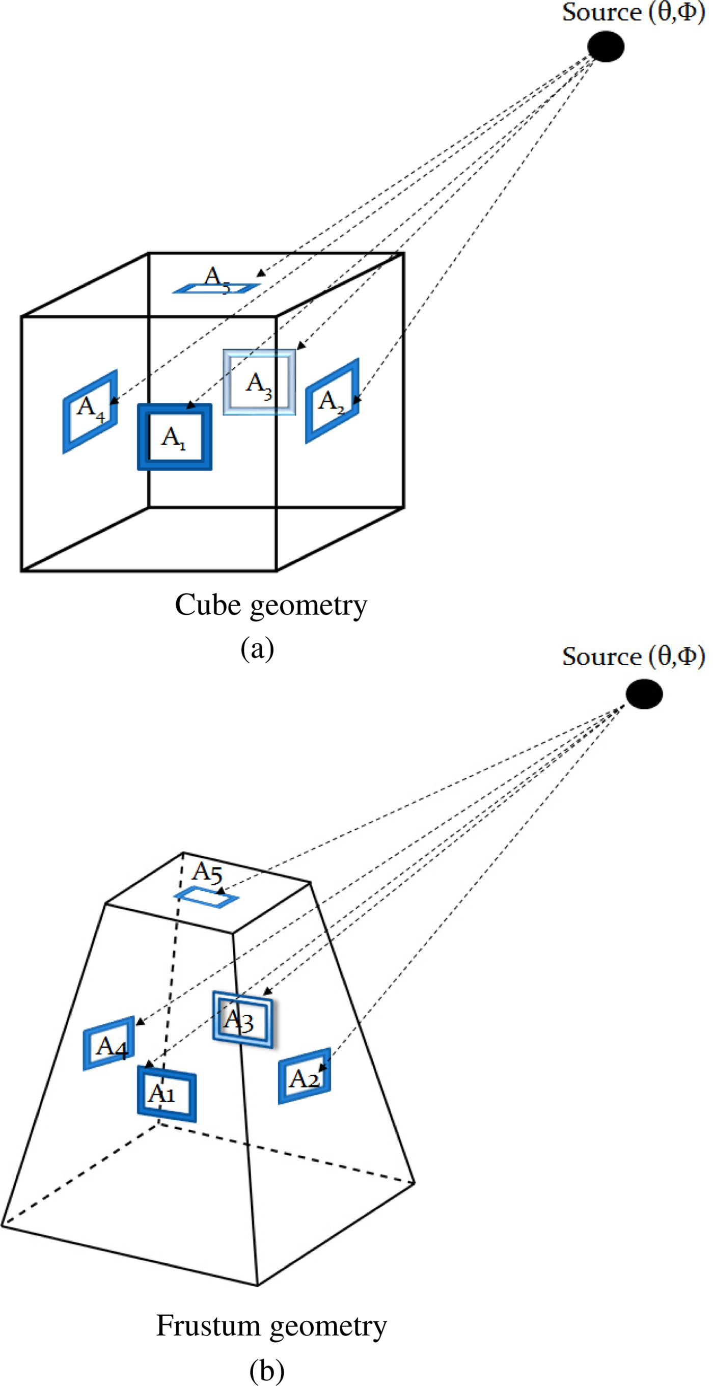
Fig. 1. Multiple antennas distributed over cube and frustum geometries for locating a radiating source. (a) Cube geometry. (b) Frustum geometry.
System model
We determine the power received on each antenna element on the face of the cube and frustum. At first, we define the global co-ordinate axes with origin at the center of the 3D solid figure. Along with this, local axes for each antenna with the center of each antenna as origin are defined. Radiation pattern of each antenna is determined with respect to the local axes of that particular antenna.
Assume a radiation source located at the global co-ordinates (θ, ϕ). We need to estimate the signal power from this source received in all five antennas of the antenna system. This requires the radiation pattern of each antenna, which essentially provides the gain of each of the receiving antenna in the direction (θ, ϕ), see Fig. 1. For this, we need to translate the source co-ordinates (θ, ϕ) to local coordinates of each antenna A k, say (x k, y k, z k), k = [1:5]. Therefore, we can compute the direction of source for each antenna as  $(\theta _A^{(k)},\phi _A^{(k)})$ using the local coordinate system of each antenna. For our simulation studies, we used microstrip patch antenna as the antenna candidate. Hence, we can use the empirical expressions of electric fields given in [Reference James and Hall26] written as,
 $$\eqalign{ E\left(\theta_A^{(k)}\right)=& \displaystyle{{{\sin\left({kW\sin{\theta_A^{(k)}}\sin{\phi_A^{(k)}}}/2\right)}} \over{\left(kW\sin{\theta_A^{(k)}}\sin{\phi_A^{(k)}}/2\right)}} \cr & \times \cos\left({kL\sin{\theta_A^{(k)}}\cos{\phi_A^{(k)}}}/2\right)\cos\phi_A^{(k)}}$$
where L and W are the effective length and width of the patch antenna respectively,  ${\theta _A^{(k)}}$ is the elevation angle of the antenna, and k is the free-space wavenumber, given by 2π/λ [Reference James and Hall26]. Similarly, radiation pattern of the patch antenna as a function of azimuth angle
  ${\phi _A^{(k)}}$ is given by,
 $$\eqalign{E\left(\phi_A^{(k)}\right)=& -\displaystyle{{{\sin\left({kW\sin{\theta_A^{(k)}}\sin{\phi_A^{(k)}}}/2\right)}} \over{\left(kW\sin{\theta_A^{(k)}}\sin{\phi_A^{(k)}}/2\right)}} \cr & \times \cos\left({kL\sin{\theta_A^{(k)}}\cos{\phi_A^{(k)}}}/2\right) \cos\theta_A^{(k)}\sin\phi_A^{(k)}}$$
The receiving antenna gain for antenna k can therefore be written as,
 $$G_R^{(k)} = E\left(\theta_A^{(k)}\right)^2 + E\left(\phi_A^{(k)}\right)^2$$
Hence, received signal power at each antenna from the electromagnetic source located at (θ, ϕ) can be computed using the Friis transmission equation [Reference Pozar27] as,
 $$P_R^{(k)}= P_{T}^{(k)}\,G_{T}^{(k)}G_{R}^{(k)} \left(\displaystyle{{\lambda} \over{4{\pi}r^{(k)}}}\right)^2$$
where r (k) is the distance between the source and the antenna A k. Thus, the received power in all antennas located on different faces of the cube and frustum can be found. Now, power at all the antennas distributed over various faces of the cube or frustum and the corresponding positions of the source can be used as training input and output of an ANN. The trained ANN can be used to predict the direction of the electromagnetic source based on the power measured on antenna elements of the antenna system.
It is to be noted that, for training, the radial distance of source r (k) in (4) can be made constant. This is because of the fact that, the structure dimensions are very small compared to the radial distance and normalized power in all the antennas becomes independent of the distance. This crucial assumption requires us to only generate a set of random positions for constant r (k).
For studying the performance of the proposed localization method, a set of data (θ i, ϕ i), i = [0:N] is generated randomly, where N represents the number of training samples. The power received in the antenna elements of the cube- and frustum-based antenna systems is determined for each training sample using (4). The ANN is trained using the received powers on each antenna element as inputs and corresponding (θ i, ϕ i) as outputs of ANN. The trained ANN with resultant weights is used for evaluating the accuracy of the proposed system. For the development of ANN, we used an open source program, Fast Artificial Neural Network Library (FANN) [28]. We tested different algorithms for training the ANN, such as, QPROP (quick propagation) and RPROP (resilient back propagation). Due to faster convergence, we selected RPROP as our training algorithm. Thus, positions and corresponding power pattern can be used as training data for ANN. The multi-antenna system configured to ANN, once trained, can process the received power pattern of different antennas corresponding to various source locations, enabling us to predict the source co-ordinates from the RSSs.
It is to be noted that, any machine learning technique for regression based on supervised learning can potentially be applied for the proposed application. Some widely used machine learning methods for supervised learning other than ANN are SVMs [Reference Smola and Scholkopf29, Reference Bae, Jang and Sung30], Logistic Regression [Reference Perlich, Provost and Simonoff31], Naive Bayes [Reference Song, Liu, Yuan and Qiu32], Random Forests [Reference Pang, George, Hui and Tong33], Bagged Trees [Reference Cordon, Quirin and Sanchez34], and Boosted Trees [Reference Lin, Shen and Hengel35]. Based on 11 test problems and eight different performance metrics, it is shown in [Reference Caruana36] that Bagged Trees, Random Forests, and ANN gave the best average performance. It is also observed in [Reference Caruana36] that SVM and newer methods such as Boosted Trees outperform ANN by applying calibration and tuning after training. However, this requires more computations. Hence, we implemented SVM- and Gradient Boosted Trees-based regression using the python package Scikit-Learn [37], to evaluate the performance of the proposed system.
Since the test data for ANN is generated by simulation, for increased accuracy, we must consider experimental uncertainties in the proposed system such as mutual coupling between the elements and channel characteristics between the electromagnetic source and individual antenna elements. Although, we used simplified formulas which are reasonably accurate, we can increase the accuracy in test data by deploying electromagnetic simulators which have evolved in its capability and accuracy over the years. Different numerical methods are embedded in electromagnetic simulators and designer can compare them for confidence in simulated results. Therefore, simulation-based approach to generate data sets for ANN will be accurate. Also the localization applications considered in the proposed method have a simple line of sight channel models. On the other hand, if we deploy the system in complex indoor or outdoor environments, we can derive the channel models experimentally and incorporate the channel models thus derived to generate reliable training and validation data for ANN.
Numerical results
Received power pattern for cube-based geometry
In our first study, we arranged the antennas in a cubical geometry as shown in Fig 1(a). The received power pattern in the multiple antennas is studied for various source locations, corresponding to different θ and ϕ.
The variation in RSS in antennas A 1, A 2, and A 3, when the source moves from ϕ equal to 0 to 360° in a plane where θ = 45°, is shown in Fig. 2. As we can see in Fig. 2, received signal power in antenna A 1 is maximum at ϕ equal to zero. Signal power decreases and touches zero around ϕ equal to 72°. Again received power in A 1 increases gradually and reaches a maximum value and sharply declines to zero and continues in that level until ϕ becomes close to 290°. Received power in A 1 exhibits a sharp shoot followed by a decline again. Then power rises gradually and forms a local peak when ϕ reaches 360°. Received power in antenna A 2 is initially at zero, but follows the same pattern like A 1. Figure 3 illustrates the variation in signal power in antennas A 4 and A 5 as the source moves from ϕ value equal to 0 to 360° in a theta plane θ = 45°. As seen in Fig. 3, antenna A 5 is always illuminated since it is located at the top face of the cube. On the other hand, Antenna A 4 shows a behavior similar to antennas A 1, A 2, and A 3 since they are located on the side faces of the cube. Hence, antennas, A k, k = [1:4] receive power for half of the cycle and cut-off for the other half. Variation pattern is same for side antennas but it is exhibited in different stages of the cycle. As we can see from Figs 2 and 3, received signal power is different in all the antennas for the same source location as it depends on the direction angle. Therefore, RSS in the multi-antenna system forms a predictable pattern according to the position of the source. Also, we can conclude that the received power pattern is unique for each source location.

Fig. 2. Received antenna power in Antennas 1, 2, and 3 when the source moves in a θ = 45° plane for cube-based antenna geometry.
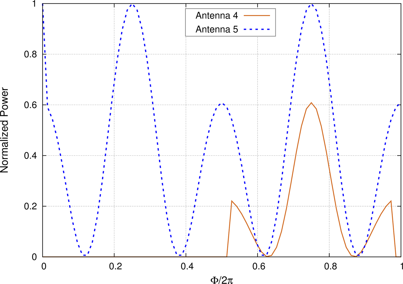
Fig. 3. Received antenna power in Antennas 4 and 5 when the source moves in a θ = 45° plane for cube-based antenna geometry.
Figure 4 shows the variation in received signal power in antennas with respect to θ for constant ϕ. The range of θ is from 0 to 180° such that source points are located in a hemisphere. We can see from Fig. 4 that the power received in top antenna A 5 is the maximum when θ is equal to zero. Received power gradually decreases and touches zero around θ equal to 45°. Again it increases and then drops back to zero at θ equal to 90°. Side antennas A 1 and A 2 are exposed to the same signal power throughout the cycle. Initially the RSS is less and increases to the maximum at θ equal to 90°. After this peak, the power gradually decreases to zero. Antennas A 3 and A 4 are completely cut-off and they do not receive any signal throughout this cycle. From Fig. 4, we can infer that signal strength varies drastically across antennas in this simulation. Antennas A 3 and A 4 are totally cut-off and not receiving any signal since their orientation is in the opposite hemisphere. Antennas A 1 and A 2 are receiving similar signal strength as they are equidistant and equally inclined to the source at all positions. Antenna A 5 is able to enhance the uniqueness of the RSS pattern as its pattern is different from rest of the antennas.
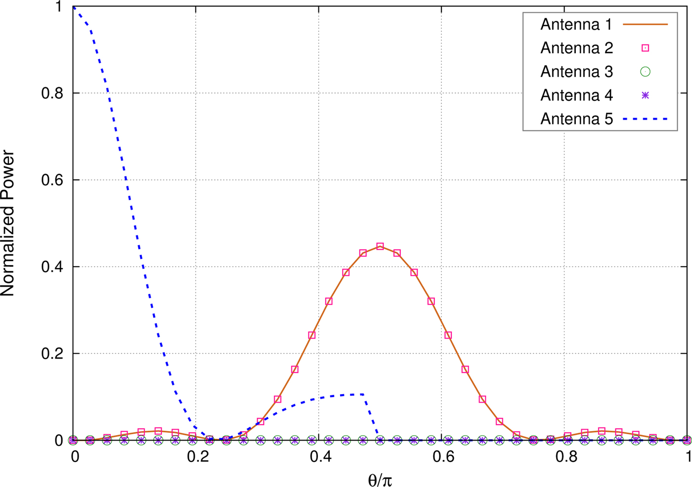
Fig. 4. Received antenna power when the source moves in a ϕ = 45° plane for cube-based antenna geometry.
Above two simulation studies give us the confidence that RSS pattern in the multi-antenna array system is unique for any source location and these data can be used to train an ANN enabling the system to predict the source location.
Accuracy of the proposed system for cube-based geometry
The performance of the proposed system is evaluated for cube-based geometry. The ANN is trained using the power patterns corresponding to the randomly generated (θ, ϕ). Figure 5 shows the variation of ANN prediction error (Root Mean Square Error (RMSE)) as the complexity of the neural network is increased in terms of the number of neurons. We started experimenting the ANN with 12 neurons, but as we can see from Fig. 5 that RMSE ≈ 0.6 for many neurons. As we increase the number of neurons, RMSE decreases to below 0.2 for 15 neurons. After 35 neurons, the reduction in RMSE is not significant and approximately remains almost constant.
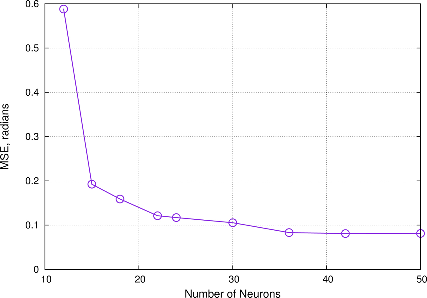
Fig. 5. Prediction accuracy versus complexity of ANN in terms of number of neurons for cube-based geometry.
The prediction accuracy of the neural network is studied by varying the number of training points and the complexity of the neural network. Fig. 6 shows the prediction error of the neural network with different sizes of training data. As we can see from Fig. 6, that prediction error of the neural network is high when the number of training points is less. As we increase the size of training data, prediction error decreases. For instance, when ANN is trained with 35,000 data points, RMSE reduces to below 0.09. Therefore, we can conclude that, the prediction error not only depends on the number of neurons but also depends on the size of training data. From both Figs 5 and 6, we can conclude that, the prediction accuracy of ANN is definitely improved by increasing the training data size and by increasing the complexity or hidden layers of the neural network in terms of the number of neurons. Table 1 gives 20 samples of actual and predicted source co-ordinates when the source is moving in a random cloud. This simulation is carried out with ANN which is modeled using 35,000 training points and with 50 neurons.
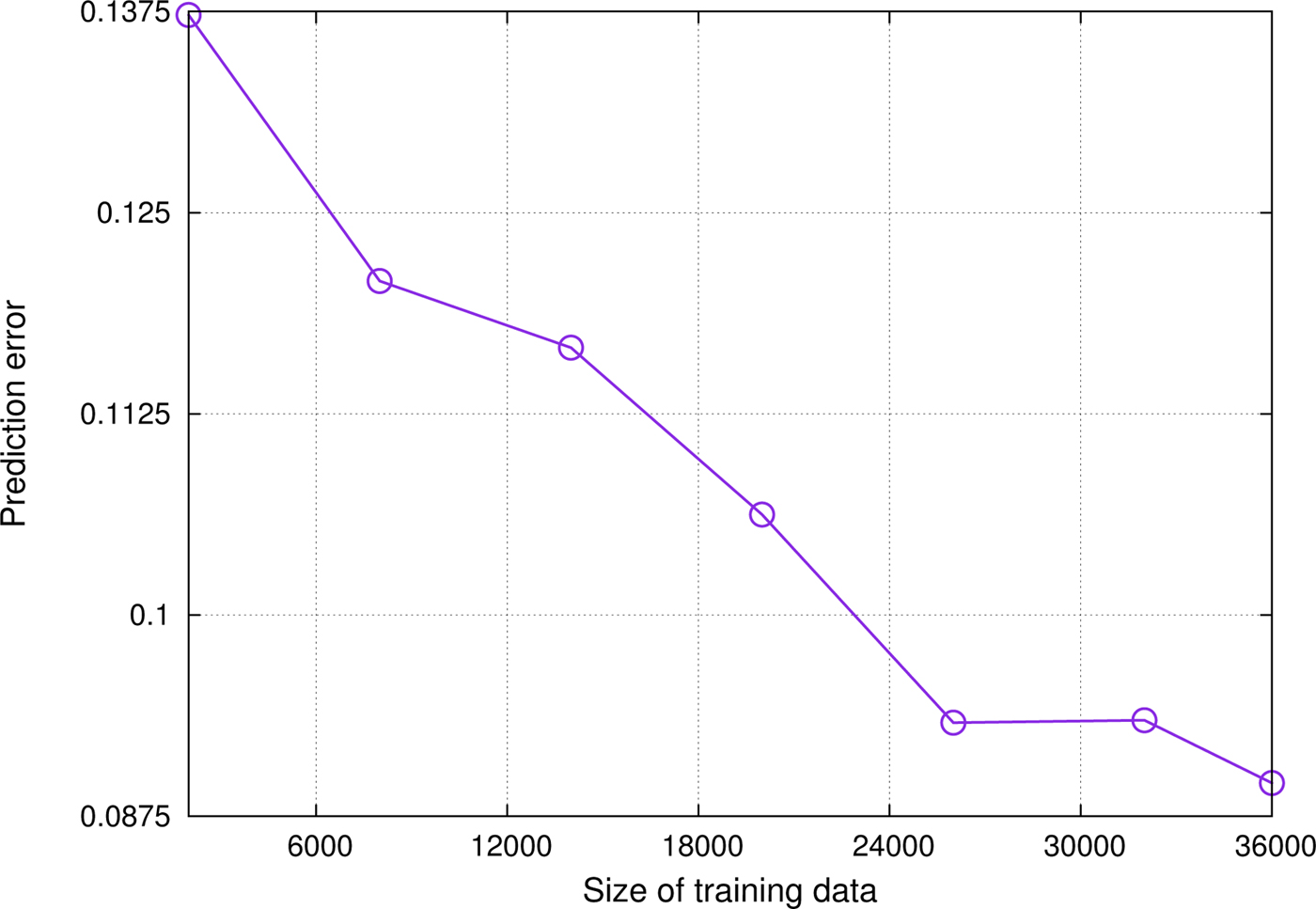
Fig. 6. Prediction accuracy versus size of ANN training data for cube-based geometry.
Table 1. Actual and predicted source locations in radians with ANN for cube geometry

Received power pattern for frustum based geometry
Above simulations are repeated for antennas arranged on frustum geometry as shown in Fig. 1(b). In frustum-based antenna geometry, four side antennas are placed on the tilted surfaces which form the faces of the frustum. For a fair comparison, frustum and cube dimensions are defined in such a way that both have similar height and dimensions of base. Figure 7 shows the variation in received power in antennas A 1, A 2, and A 3, when the source moves corresponding to ϕ spanning from 0 to 360° in a theta plane (θ = 45°). We observe a ripple power pattern in all the antennas throughout the cycle of ϕ variation. It is also observed that though the signal strength is different in antennas for same source location, they appear to be more close. Figure 8 illustrates the variation in signal power in antennas A 4 and A 5 as the source moves from ϕ value equal to 0 to 360° in a theta plane. As seen in Fig. 8, antenna A 5 is always illuminated since it is located at the top face of the cube. Power in A 4 is initially zero as ϕ changes from zero to 180°. Then the signal strength increases and reaches a local peak and declines to zero as ϕ reaches 360°. As we can see from Figs 7 and 8, received signal power is different in all the antennas for the same source location. These characteristics are similar to the results what we have seen in the cube-based geometry, see Figs 2 and 3. But in the case of frustum, we observe that more number of antennas are exposed to the signal from the radiating source in any given direction. Signal power in antennas appears to be more correlated due to the slanting position of antennas resulting in the more signal exposure.

Fig. 7. Received antenna power in Antennas 1, 2, and 3 when the source moves in a θ = 45° plane for frustum-based antenna geometry.

Fig. 8. Received antenna power in Antennas 4 and 5 when the source moves in a θ = 45° plane for frustum-based antenna geometry.
Figure 9 shows the variation in received signal power in antennas with respect to θ in a ϕ plane. We conclude that geometrical nature of frustum makes the received power in multi-antenna system more correlated.

Fig. 9. Received antenna power when the source moves in a ϕ = 45° plane for frustum-based antenna geometry.
Accuracy of the proposed system for frustum-based geometry
We generate random training points for ANN and compare the results between cube-based and frustum-based geometries. Table 2 gives 20 samples of actual and predicted source location co-ordinates when the source is moving in a random cloud. This simulation study is carried out with ANN which is modeled using 35000 training points and with 50 neurons.
Table 2. Actual and predicted source locations in radians with ANN for frustum geometry

Figure 10 shows the comparison between cube and frustum in terms of the complexity of neural network. In Fig. 10, we see that RMSE is almost the same for both geometries when the complexity of ANN is less, but the difference gets higher as the number of neurons is increased. Cube-based system is able to bring down the prediction error below 0.09 using an ANN with 30 neurons. But frustum-based antenna system fails to reduce the error below 0.15 even at much higher number of neurons in ANN. We can conclude that prediction becomes easier with cube-based antenna geometry as we increase the complexity of ANN. This is because, frustum geometry has more signal exposure in all directions compared to cube-based antenna system, resulting in more correlated signals in all antennas for frustum compared to the cube-based system.

Fig. 10. Comparison between cube-based and frustum-based array geometries with respect to the complexity of neural network.
Performance comparison
We compare the accuracy and computational runtime of the proposed ANN-based method with SVM using different kernels and Gradient Boosting Trees methods using the python package Scikit-Learn [37]. Table 3 compares the prediction RMSE of θ and ϕ using different regression methods. The table also compares the computational runtime of each method to obtain the mentioned accuracies. As we can see from Table 3, the runtimes are lower for ANN. On the other hand, SVM and Gradient Boosted methods provide greater accuracy when compared to the ANN method, but at the cost of higher runtime. Of the SVM-based methods, Radial Basis function kernel provides in general higher accuracy with higher runtime. When comparing with SVM-based methods, Boosted Trees method provides higher accuracy and better runtime. From Table 3, we can conclude that, the proposed ANN-based method provides optimum accuracy with lower runtime when compared to other regression methods.
Table 3. RMSE comparison of the proposed ANN-based method with SVM- and Gradient Boosting Trees-based regression methods

We further compare our numerical results with the experimental results of [Reference Tidd, Raymond, Huang and Zhao17]. The study of [Reference Tidd, Raymond, Huang and Zhao17] extends a temporal domain ESPRIT frequency estimation algorithm for the estimation of azimuth and elevation angle. A maximum tracking error of 11 degrees is reported using Kalman-based tracking. The error is calculated as the difference between estimated DOA and MUSIC algorithm-based DOA. As we can see from Table 3, the proposed system provides accuracies comparable with the experimental results of [Reference Tidd, Raymond, Huang and Zhao17] using different regression methods.
Conclusion
A new method for identifying the location of an electromagnetic source using 3D antenna array systems was proposed and tested in this paper. The ANN-based system was able to predict the source location using RSS pattern in antennas. Two geometries for generating RSS data are considered, namely the cube-based and the frustum-based multi-antenna system. From the simulated results, we can conclude that the proposed method has higher accuracy for the cube-based antenna system compared to that of frustum.
Author ORCIDs
Dhanesh G. Kurup, 0000-0003-1998-4997
 Sreenivasulu Pala received his B.Tech degree in electronics and communication engineering from Jawaharlal Nehru Technological University, Hyderabad, India in 2003. He received his M.E degree in applied electronics from Sathyabama Institute of Science and Technology, Chennai, India in 2005. He joined Robert Bosch Engineering and Business Solutions Limited, Bangalore, India in 2005 and is currently working as a senior architect. He is pursuing his Ph.D. at Amrita School of Engineering, Amrita University, Bangalore, India from 2013. His research interests include indoor localization and machine learning.
 Srividhya P received her Bachelor's degree in electronics and communication engineering from the University of Calicut, India in 2000. She received her Master's degree in Communication Engineering and Signal processing from Amrita School of Engineering, Amrita University, Bangalore, India in 2017. She is currently working as a Principal Educator in an Information Technology firm. Her research interests include digital signal processing.
 Mohamed Himdi received the Ph.D. degree in signal processing and telecommunications from the University of Rennes 1, France, in 1990. Since 2003, he has been a Professor with the University of Rennes 1, and the Head of the High Frequency and Antenna Department until 2013, of IETR. He has authored or co-authored 112 journal papers and over 255 papers in conference proceedings. He has also co-authored nine book chapters. He holds 39 patents. His research activities concern passive and active millimeter-wave antennas. His research also includes the development of new architectures of antenna arrays, and new 3D antenna technologies. He was a Laureat of the 2D National Competition for the Creation of Enterprises in Innovative Technologies, in 2000 (Ministry of Industry and Education). In 2015, he was a recipient of the JEC-AWARD at Paris on pure composite material antenna embedded into a motorhome roof for the digital terrestrial television reception.
 Olivier Lafond received the M.S. degree in radar and telecommunications and the Ph.D. degree in signal processing and telecommunications from the University of Rennes 1, Rennes, France, in 1996 and 2000, respectively. Since 2002, he has been an Associate Professor with the Institute of Electronics and Telecommunications of Rennes, University of Rennes 1. He has authored or co-authored 40 journal papers and 63 papers in conference proceedings. He has also authored/co-authored three book chapters. He holds seven patents in the area of antennas. His research activities deal with passive and active millimeter-wave multilayer antennas and circuits, reconfigurable antennas, inhomogeneous lenses for shaping radiation patterns with active devices, and imaging antenna systems.
 Dhanesh G. Kurup received his Bachelor's and Master's degrees in Electronics and Communication Engineering from Calicut University and Indian Institute of Technology, Roorkee, India, respectively. He further obtained Ph.D. degrees from Uppsala University, Sweden and University of Rennes 1, France. He was with the Satellite Centre, Indian Space Research Organization (ISRO), Bangalore as a Scientist/Engineer for about 2 years and as a Guest Researcher with the University of Rennes for about 3 years. For about 8 years, he directed research and subsequently as a consultant for about 1 year at Wavelogics AB, Sweden. In addition, he has teaching experience of over 4 years. His research interests includes active antennas, antenna arrays, computational electromagnetics, RF circuit design, signal processing, and behavioral modeling of wireless systems.


