


1 Introduction
Decaying or stochastically forced two-dimensional (2-D) turbulence in the presence of rigid boundaries is characterised by self-organised coherent structures. For a square domain (Clercx, Maassen & Van Heijst Reference Clercx, Maassen and Van Heijst1998; Molenaar, Clercx & Van Heijst Reference Molenaar, Clercx and Van Heijst2004), a spontaneous spin-up is observed which leads to the formation of a single vortex structure. This structure can persist for very long periods of time, before suddenly breaking and reorganising itself, in some cases with a reversed rotation sense. A similar process occurs in the geomagnetic field under the form of polarity switches (Wicht, Stellmach & Harder Reference Wicht, Stellmach and Harder2009; Valet et al. Reference Valet, Fournier, Courtillot and Herrero-Bervera2012). In turbulent Rayleigh–Bénard (RB) convection experiments, this phenomenon is also observed: a large-scale circulation (LSC), commonly referred to as the wind, changes sign intermittently. Several models have been proposed to describe this process in RB convection through either stochastic differential equations (Sreenivasan, Bershadskii & Niemela Reference Sreenivasan, Bershadskii and Niemela2002; Benzi Reference Benzi2005; Brown & Ahlers Reference Brown and Ahlers2007; Podvin & Sergent Reference Podvin and Sergent2015) or phenomenological and physically motivated assumptions (Araujo, Grossmann & Lohse Reference Araujo, Grossmann and Lohse2005; Resagk et al. Reference Resagk, du Puits, Thess, Dolzhansky, Grossmann, Fontenele Araujo and Lohse2006; Brown & Ahlers Reference Brown and Ahlers2007).
The LSC structure, its global properties and the transition between dominant flow structures are found to be dependent on the cavity shape (Grossmann & Lohse Reference Grossmann and Lohse2003; Xi & Xia Reference Xi and Xia2008b
; van der Poel, Stevens & Lohse Reference van der Poel, Stevens and Lohse2011). Inside cylindrical cells, a change of sign of the LSC occurs either by a rotation-led reversal through an azimuthal rotation of the near-vertical circulation plane known as azimuthal meandering, or by a cessation-led reversal through the breakdown of the existing LSC before reorganising in a different spatial direction (see, for instance, Niemela et al.
Reference Niemela, Skrbek, Sreenivasan and Donnelly2001, Sreenivasan et al.
Reference Sreenivasan, Bershadskii and Niemela2002, Brown & Ahlers Reference Brown and Ahlers2007, Funfschilling, Brown & Ahlers Reference Funfschilling, Brown and Ahlers2008, Xi & Xia Reference Xi and Xia2008a
,Reference Xi and Xia
b
). One approach to separate rotation-led from cessation-led reversal events consists in restricting the experimental study to a square box of small aspect ratio in the transversal direction (Xia, Sun & Zhou Reference Xia, Sun and Zhou2003; Sugiyama et al.
Reference Sugiyama, Ni, Stevens, Chan, Zhou, Xi, Sun, Grossmann, Xia and Lohse2010; Wagner & Shishkina Reference Wagner and Shishkina2013; Ni, Huang & Xia Reference Ni, Huang and Xia2015). Another viewpoint uses 2-D direct numerical simulations (Sugiyama et al.
Reference Sugiyama, Ni, Stevens, Chan, Zhou, Xi, Sun, Grossmann, Xia and Lohse2010; Chandra & Verma Reference Chandra and Verma2011; Petschel et al.
Reference Petschel, Wilczek, Breuer, Friedrich and Hansen2011; Podvin & Sergent Reference Podvin and Sergent2015; Verma, Ambhire & Pandey Reference Verma, Ambhire and Pandey2015) since rotation-led reversals are not possible in such a configuration. However, it is not entirely clear whether 2-D reversals and cessation-led reversals correspond to the same phenomenon. Sugiyama et al. (Reference Sugiyama, Ni, Stevens, Chan, Zhou, Xi, Sun, Grossmann, Xia and Lohse2010) have identified a region in the (
 $Ra$
,
$Ra$
,
 $Pr$
) space in which reversal events are observed experimentally inside quasi-2-D cells as well as numerically in 2-D simulations. For this range of (
$Pr$
) space in which reversal events are observed experimentally inside quasi-2-D cells as well as numerically in 2-D simulations. For this range of (
 $Ra,Pr$
), the flow inside a square cell is mainly composed of a large diagonal roll and two counter-rotating corner rolls. Sugiyama et al. (Reference Sugiyama, Ni, Stevens, Chan, Zhou, Xi, Sun, Grossmann, Xia and Lohse2010) and Chandra & Verma (Reference Chandra and Verma2013) pointed out the feeding of corner rolls by plumes detached from horizontal boundary layers. Both papers proposed that the growth of corner rolls ended by a sudden LSC transition.
$Ra,Pr$
), the flow inside a square cell is mainly composed of a large diagonal roll and two counter-rotating corner rolls. Sugiyama et al. (Reference Sugiyama, Ni, Stevens, Chan, Zhou, Xi, Sun, Grossmann, Xia and Lohse2010) and Chandra & Verma (Reference Chandra and Verma2013) pointed out the feeding of corner rolls by plumes detached from horizontal boundary layers. Both papers proposed that the growth of corner rolls ended by a sudden LSC transition.
The presence of such coherent structures has been investigated by computing the first Fourier modes (Chandra & Verma Reference Chandra and Verma2011; Verma et al. Reference Verma, Ambhire and Pandey2015), or by obtaining these modes from a proper orthogonal decomposition (Bailon-Cuba, Emran & Schumacher Reference Bailon-Cuba, Emran and Schumacher2010; Podvin & Sergent Reference Podvin and Sergent2015). Coherent structures are actually associated with a sum of various such modes: a large-scale monopole, a quadrupole and a vertically or horizontally stacked dipole. A study of the transition sequences between these first Fourier modes indicated the presence of a reversal path (Petschel et al. Reference Petschel, Wilczek, Breuer, Friedrich and Hansen2011). To analyse such a process, one could adopt the perspective used in geomagnetic fields combining a careful selection of reversal records as well as a time rescaling (Valet et al. Reference Valet, Fournier, Courtillot and Herrero-Bervera2012; Lhuillier, Hulot & Gallet Reference Lhuillier, Hulot and Gallet2013). In geomagnetism, this method led to the definition of three successive phases: a precursory event, a polarity switch and a rebound.
Another viewpoint is based on energetic considerations. For instance, available potential energy is key to understanding how mechanical energy is transported, stored and dissipated in RB convection (Winters et al. Reference Winters, Lombard, Riley and D’Asaro1995; Hughes, Gayen & Griffiths Reference Hughes, Gayen and Griffiths2013). This approach could make more precise the idea of an avalanche mechanism (mentioned in Sreenivasan et al. Reference Sreenivasan, Bershadskii and Niemela2002), due to a localised accumulation of energy, which increases local gradients until a certain threshold is reached and energy is expelled as a single burst.
In the present paper, we propose for RB convection, a formulation similar to the one proposed in geomagnetism (Valet et al. Reference Valet, Fournier, Courtillot and Herrero-Bervera2012): the main objective is to establish the existence of a generic reversal cycle and to identify in this cycle three phases (release, accumulation and acceleration). This analysis combines a statistical analysis with a physical approach relying on the angular momentum as well as kinetic and potential energy to highlight the underlying physical mechanisms. In addition, we identify flow patterns corresponding to each phase of the generic cycle by using a conditional averaging. A threshold state in generic reversal cycles is identified from which the release is inevitable.
The paper is organised as follows. Section 2 introduces the model equations and global quantities: global angular impulse, available mechanical energy and corresponding conversion rates. A brief description of the numerical method and the spatial resolution is presented in § 3. In § 4, a filtering method is proposed that identifies two regimes, and then allows us to perform a statistical study of reversals. The dynamics of a generic reversal mechanism is described as composed by three phases in § 5. These results are then analysed in terms of coherent flow structures and physical mechanisms in § 6 for particular realisations. In § 7, a stability analysis is applied on the generic cycle. Section 8 contains a brief comparison of the present analysis with previous works. Finally, some prospective works are mentioned in conclusion.
2 Model equations and analysis tools
Consider a fluid contained in a square cell, cooled at the top with constant temperature
 $T_{top}$
and heated at the bottom with constant temperature
$T_{top}$
and heated at the bottom with constant temperature
 $T_{bot}>T_{top}$
. The flow equations are based on the Boussinesq approximation. The flow regime is defined as a function of the Rayleigh and Prandtl numbers,
$T_{bot}>T_{top}$
. The flow equations are based on the Boussinesq approximation. The flow regime is defined as a function of the Rayleigh and Prandtl numbers,
 $$\begin{eqnarray}Ra\equiv \frac{gH^{3}\unicode[STIX]{x1D6FD}\left(T_{bot}-T_{top}\right)}{\unicode[STIX]{x1D705}\unicode[STIX]{x1D708}},\quad Pr\equiv \frac{\unicode[STIX]{x1D708}}{\unicode[STIX]{x1D705}}\end{eqnarray}$$
where
 $g$
denotes gravity,
$g$
denotes gravity,
 $H$
the cell height and
$H$
the cell height and
 $\unicode[STIX]{x1D6FD}$
,
$\unicode[STIX]{x1D6FD}$
,
 $\unicode[STIX]{x1D705}$
,
$\unicode[STIX]{x1D705}$
,
 $\unicode[STIX]{x1D708}$
are respectively volumetric thermal expansion, thermal diffusivity and kinematic viscosity coefficients. The values of
$\unicode[STIX]{x1D708}$
are respectively volumetric thermal expansion, thermal diffusivity and kinematic viscosity coefficients. The values of
 $(Ra,Pr)$
used for direct numerical simulations (DNS) correspond to a weakly turbulent flow regime where reversals have been reported (Sugiyama et al.
Reference Sugiyama, Ni, Stevens, Chan, Zhou, Xi, Sun, Grossmann, Xia and Lohse2010). As far as notations are concerned,
$(Ra,Pr)$
used for direct numerical simulations (DNS) correspond to a weakly turbulent flow regime where reversals have been reported (Sugiyama et al.
Reference Sugiyama, Ni, Stevens, Chan, Zhou, Xi, Sun, Grossmann, Xia and Lohse2010). As far as notations are concerned,
 $x$
(respectively
$x$
(respectively
 $u$
) and
$u$
) and
 $y$
(respectively
$y$
(respectively
 $v$
) stand for the horizontal and vertical directions (respectively velocities). Coordinate vector
$v$
) stand for the horizontal and vertical directions (respectively velocities). Coordinate vector
 $\boldsymbol{x}=(x,y)$
is equal to
$\boldsymbol{x}=(x,y)$
is equal to
 $(0,0)$
at the cavity centre. One introduces the reduced temperature
$(0,0)$
at the cavity centre. One introduces the reduced temperature
 $\unicode[STIX]{x1D703}(\boldsymbol{x},t)\equiv (T-T_{0})/(T_{bot}-T_{top})$
, with
$\unicode[STIX]{x1D703}(\boldsymbol{x},t)\equiv (T-T_{0})/(T_{bot}-T_{top})$
, with
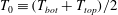 $T_{0}\equiv (T_{bot}+T_{top})/2$
as well as the only vorticity component
$T_{0}\equiv (T_{bot}+T_{top})/2$
as well as the only vorticity component
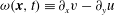 $\unicode[STIX]{x1D714}(\boldsymbol{x},t)\equiv \unicode[STIX]{x2202}_{x}v-\unicode[STIX]{x2202}_{y}u$
. For a field
$\unicode[STIX]{x1D714}(\boldsymbol{x},t)\equiv \unicode[STIX]{x2202}_{x}v-\unicode[STIX]{x2202}_{y}u$
. For a field
 $a(\boldsymbol{x},t)$
, the fields
$a(\boldsymbol{x},t)$
, the fields
 $\overline{a}(\boldsymbol{x})$
and
$\overline{a}(\boldsymbol{x})$
and
 $\unicode[STIX]{x1D70E}(a)(\boldsymbol{x})$
denote the time average and standard deviation computed using the full long-term time series. In addition, quantity
$\unicode[STIX]{x1D70E}(a)(\boldsymbol{x})$
denote the time average and standard deviation computed using the full long-term time series. In addition, quantity
 $\langle a\rangle _{vol}(t)$
stands for the volume average of
$\langle a\rangle _{vol}(t)$
stands for the volume average of
 $a(\boldsymbol{x},t)$
.
$a(\boldsymbol{x},t)$
.
Based on the cell height
 $H$
as characteristic length scale and
$H$
as characteristic length scale and
 $\unicode[STIX]{x1D705}\sqrt{(Ra)}/H$
as velocity scale, the dimensionless velocity
$\unicode[STIX]{x1D705}\sqrt{(Ra)}/H$
as velocity scale, the dimensionless velocity
 $\boldsymbol{u}=(u,v)$
and reduced temperature
$\boldsymbol{u}=(u,v)$
and reduced temperature
 $\unicode[STIX]{x1D703}$
satisfy the dimensionless system of equations
$\unicode[STIX]{x1D703}$
satisfy the dimensionless system of equations
 $$\begin{eqnarray}\left.\begin{array}{@{}rcl@{}}\!\unicode[STIX]{x1D735}\boldsymbol{\cdot }\boldsymbol{u}\ & =\ & 0,\\ \!\unicode[STIX]{x2202}_{t}\boldsymbol{u}+\unicode[STIX]{x1D735}\boldsymbol{\cdot }[\boldsymbol{u}\otimes \boldsymbol{u}]\ & =\ & -\unicode[STIX]{x1D735}p+Pr\,Ra^{-0.5}\unicode[STIX]{x1D735}^{2}\boldsymbol{u}+Pr\unicode[STIX]{x1D703}\boldsymbol{e}_{y},\\ \!\unicode[STIX]{x2202}_{t}\unicode[STIX]{x1D703}+\unicode[STIX]{x1D735}\boldsymbol{\cdot }[\boldsymbol{u}\unicode[STIX]{x1D703}]\ & =\ & Ra^{-0.5}\unicode[STIX]{x1D735}^{2}\unicode[STIX]{x1D703}.\end{array}\right\}\end{eqnarray}$$
A no-slip condition for the velocity field is ensured on the walls. On the top (respectively bottom) walls, one imposes
 $\unicode[STIX]{x1D703}=-0.5$
(respectively
$\unicode[STIX]{x1D703}=-0.5$
(respectively
 $\unicode[STIX]{x1D703}=0.5$
) while adiabaticity
$\unicode[STIX]{x1D703}=0.5$
) while adiabaticity
 $\unicode[STIX]{x2202}_{x}\unicode[STIX]{x1D703}=0$
is satisfied on side walls. From now on, quantities are written in dimensionless form only.
$\unicode[STIX]{x2202}_{x}\unicode[STIX]{x1D703}=0$
is satisfied on side walls. From now on, quantities are written in dimensionless form only.
2.1 Global angular impulse
The global angular momentum
 $$\begin{eqnarray}L_{2D}(t)\equiv -\frac{1}{2}\int \boldsymbol{x}^{2}\unicode[STIX]{x1D714}(\boldsymbol{x},t)\,\text{d}x\,\text{d}y\end{eqnarray}$$
serves as a measure of organised rotation (see for instance Molenaar et al.
Reference Molenaar, Clercx and Van Heijst2004). Figure 1 shows a time series of the normalised angular momentum
 $L_{2D}/\overline{|L_{2D}|}$
. Two different regimes are observed. Blue areas correspond to periods of time where
$L_{2D}/\overline{|L_{2D}|}$
. Two different regimes are observed. Blue areas correspond to periods of time where
 $L_{2D}$
changes sign spontaneously over time: positive (respectively negative) peaks in
$L_{2D}$
changes sign spontaneously over time: positive (respectively negative) peaks in
 $L_{2D}$
alternate that are associated with a dominant counter-clockwise (respectively clockwise) central vortex. The blue areas consisting of a sequence of consecutive transitions is hereafter called the consecutive reversal (CR) regime. Outside this regime, the LSC is no longer well defined and one observes an extended cessation. Such complementary region is denoted here as the extended cessation (EC) regime.
$L_{2D}$
alternate that are associated with a dominant counter-clockwise (respectively clockwise) central vortex. The blue areas consisting of a sequence of consecutive transitions is hereafter called the consecutive reversal (CR) regime. Outside this regime, the LSC is no longer well defined and one observes an extended cessation. Such complementary region is denoted here as the extended cessation (EC) regime.

Figure 1. Time evolution of
 $L_{2D}(t)/\overline{|L_{2D}|}$
shown for (
$L_{2D}(t)/\overline{|L_{2D}|}$
shown for (
 $Ra=5\times 10^{7}$
,
$Ra=5\times 10^{7}$
,
 $Pr=3$
). Light blue areas correspond to a consecutive reversal (CR) regime, while blank areas correspond to an extended cessation (EC) regime. Some events (darker blue areas) may not be clearly assigned to the CR regime, see text. The two continuous lines correspond to the thresholds used by the filtering procedure. Value of the normalised standard deviation:
$Pr=3$
). Light blue areas correspond to a consecutive reversal (CR) regime, while blank areas correspond to an extended cessation (EC) regime. Some events (darker blue areas) may not be clearly assigned to the CR regime, see text. The two continuous lines correspond to the thresholds used by the filtering procedure. Value of the normalised standard deviation:
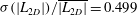 $\unicode[STIX]{x1D70E}(|L_{2D}|)/\overline{|L_{2D}|}=0.499$
.
$\unicode[STIX]{x1D70E}(|L_{2D}|)/\overline{|L_{2D}|}=0.499$
.
In order to differentiate in a precise manner the CR regime from the EC regime, a filtering algorithm has been devised which is modelled after (Lhuillier et al.
Reference Lhuillier, Hulot and Gallet2013; Podvin & Sergent Reference Podvin and Sergent2015). We identify the set of consecutive times
 $r_{i}$
at which
$r_{i}$
at which
 $L_{2D}$
changes sign. The time interval
$L_{2D}$
changes sign. The time interval
 $[r_{i},r_{i+1}]$
is considered to be inside the CR regime if, during this interval, the value of
$[r_{i},r_{i+1}]$
is considered to be inside the CR regime if, during this interval, the value of
 $|L_{2D}|$
reaches at least once the threshold value
$|L_{2D}|$
reaches at least once the threshold value
 $\overline{|L_{2D}|}+\unicode[STIX]{x1D70E}(|L_{2D}|)$
(light blue area in figure 1). A time interval where such threshold is not reached can be of two kinds corresponding to the darker blue areas or the white areas in figure 1. The first kind is sandwiched between two CR intervals and corresponds to a ‘rogue’ reversal, which likely belongs to the CR regime but has been filtered out by our criterion (the criteria for the selection of events in the CR regime is rather stringent as seen from the ‘rogue’ events displayed in figure 1). The second type, displayed in white, corresponds to an extended cessation.
$\overline{|L_{2D}|}+\unicode[STIX]{x1D70E}(|L_{2D}|)$
(light blue area in figure 1). A time interval where such threshold is not reached can be of two kinds corresponding to the darker blue areas or the white areas in figure 1. The first kind is sandwiched between two CR intervals and corresponds to a ‘rogue’ reversal, which likely belongs to the CR regime but has been filtered out by our criterion (the criteria for the selection of events in the CR regime is rather stringent as seen from the ‘rogue’ events displayed in figure 1). The second type, displayed in white, corresponds to an extended cessation.
For any interval
 $[r_{i},r_{i+1}]$
, its duration
$[r_{i},r_{i+1}]$
, its duration
 $\unicode[STIX]{x1D70F}_{1,i}\equiv r_{i+1}-r_{i}$
is also computed. When both intervals
$\unicode[STIX]{x1D70F}_{1,i}\equiv r_{i+1}-r_{i}$
is also computed. When both intervals
 $[r_{i-1},r_{i}]$
and
$[r_{i-1},r_{i}]$
and
 $[r_{i},r_{i+1}]$
are inside a CR regime, the duration
$[r_{i},r_{i+1}]$
are inside a CR regime, the duration
 $\unicode[STIX]{x1D70F}_{d,i}$
of the jump occurring around time
$\unicode[STIX]{x1D70F}_{d,i}$
of the jump occurring around time
 $r_{i}$
between a clockwise and counter-clockwise central vortex or vice versa can be evaluated. It is computed by identifying the times located just before and just after time
$r_{i}$
between a clockwise and counter-clockwise central vortex or vice versa can be evaluated. It is computed by identifying the times located just before and just after time
 $r_{i}$
such that
$r_{i}$
such that
 $|L_{2D}|$
reaches the threshold value
$|L_{2D}|$
reaches the threshold value
 $\overline{|L_{2D}|}-\unicode[STIX]{x1D70E}(|L_{2D}|)$
.
$\overline{|L_{2D}|}-\unicode[STIX]{x1D70E}(|L_{2D}|)$
.
 $\unicode[STIX]{x1D70F}_{d,i}$
is simply the time lapse between these two events.
$\unicode[STIX]{x1D70F}_{d,i}$
is simply the time lapse between these two events.
The change of the global angular momentum
 $L_{2D}$
may be better understood considering the relation directly obtained from the governing equation (2.2),
$L_{2D}$
may be better understood considering the relation directly obtained from the governing equation (2.2),
 $$\begin{eqnarray}\frac{\text{d}L_{2D}}{\text{d}t}=M+I_{a}-I_{b}\quad \left\{\begin{array}{@{}rcl@{}}M(t)\ & \equiv \ & \displaystyle \frac{1}{2}Pr\int \boldsymbol{x}^{2}~\unicode[STIX]{x2202}_{x}\unicode[STIX]{x1D703}\,\text{d}x\,\text{d}y\\ I_{a}(t)\ & \equiv \ & \displaystyle Pr\,Ra^{-0.5}\oint [\boldsymbol{x}\boldsymbol{\cdot }\boldsymbol{n}]~\unicode[STIX]{x1D714}\,\text{d}l\\ I_{b}(t)\ & \equiv \ & \displaystyle \frac{1}{2}Pr\,Ra^{-0.5}\oint \boldsymbol{x}^{2}~\boldsymbol{n}\boldsymbol{\cdot }\unicode[STIX]{x1D735}\unicode[STIX]{x1D714}\,\text{d}l\end{array}\right.\end{eqnarray}$$
where
 $\boldsymbol{n}$
stands for the outwards unit normal vector to the domain boundary and
$\boldsymbol{n}$
stands for the outwards unit normal vector to the domain boundary and
 $\text{d}l$
for a contour line differential element. Note that it is assumed that line integrals are performed in a counter-clockwise direction. The angular momentum thus evolves because of a bulk forcing term
$\text{d}l$
for a contour line differential element. Note that it is assumed that line integrals are performed in a counter-clockwise direction. The angular momentum thus evolves because of a bulk forcing term
 $M(t)$
known as the input torque (Molenaar et al.
Reference Molenaar, Clercx and Van Heijst2004) and two boundary integral terms
$M(t)$
known as the input torque (Molenaar et al.
Reference Molenaar, Clercx and Van Heijst2004) and two boundary integral terms
 $I_{a}(t)$
and
$I_{a}(t)$
and
 $I_{b}(t)$
.
$I_{b}(t)$
.
 $I_{b}(t)$
is close, but not identical, to the integrated vorticity flux over the domain boundary. For a square cavity, the boundary term
$I_{b}(t)$
is close, but not identical, to the integrated vorticity flux over the domain boundary. For a square cavity, the boundary term
 $I_{a}(t)$
simplifies to
$I_{a}(t)$
simplifies to
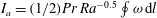 $I_{a}=(1/2)Pr\,Ra^{-0.5}\oint \unicode[STIX]{x1D714}\,\text{d}l$
. Vorticity on the boundary is related to the friction exerted by the fluid on the walls. This integral
$I_{a}=(1/2)Pr\,Ra^{-0.5}\oint \unicode[STIX]{x1D714}\,\text{d}l$
. Vorticity on the boundary is related to the friction exerted by the fluid on the walls. This integral
 $I_{a}(t)$
is thus quantifying the friction along the boundary.
$I_{a}(t)$
is thus quantifying the friction along the boundary.
2.2 Mechanical energy balance
Other global quantities are useful to characterise at each time the instantaneous state of the system: the global kinetic energy
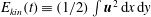 $E_{kin}(t)\equiv (1/2)\int \boldsymbol{u}^{2}\,\text{d}x\,\text{d}y$
and the global potential energy
$E_{kin}(t)\equiv (1/2)\int \boldsymbol{u}^{2}\,\text{d}x\,\text{d}y$
and the global potential energy
 $E_{pot}(t)\equiv -Pr\int y\unicode[STIX]{x1D703}\,\text{d}x\,\text{d}y$
. This latter quantifies the energy required to bring all fluid particles against gravity from their position at time
$E_{pot}(t)\equiv -Pr\int y\unicode[STIX]{x1D703}\,\text{d}x\,\text{d}y$
. This latter quantifies the energy required to bring all fluid particles against gravity from their position at time
 $t$
to the reference level
$t$
to the reference level
 $y=0$
. However, one can introduce a more pertinent instantaneous quantity, namely the available potential energy (Sutherland Reference Sutherland2010), which is defined below. For a given time
$y=0$
. However, one can introduce a more pertinent instantaneous quantity, namely the available potential energy (Sutherland Reference Sutherland2010), which is defined below. For a given time
 $t$
, the fluid is characterised by an instantaneous temperature field
$t$
, the fluid is characterised by an instantaneous temperature field
 $\unicode[STIX]{x1D703}(x,y,t)$
with a lower (respectively upper) bound at
$\unicode[STIX]{x1D703}(x,y,t)$
with a lower (respectively upper) bound at
 $\unicode[STIX]{x1D703}_{min}$
(respectively
$\unicode[STIX]{x1D703}_{min}$
(respectively
 $\unicode[STIX]{x1D703}_{max}$
). Let us consider a one-to-one mapping
$\unicode[STIX]{x1D703}_{max}$
). Let us consider a one-to-one mapping
 $(x_{r}(x,y),y_{r}(x,y))$
from the square onto the square. This may be interpreted as a reordering of fluid particles inside the square cell. Rearranging modifies the temperature field leading to a new field
$(x_{r}(x,y),y_{r}(x,y))$
from the square onto the square. This may be interpreted as a reordering of fluid particles inside the square cell. Rearranging modifies the temperature field leading to a new field
 $\unicode[STIX]{x1D703}_{r}(x,y,t)$
but this process is an adiabatic one i.e.
$\unicode[STIX]{x1D703}_{r}(x,y,t)$
but this process is an adiabatic one i.e.
 $\unicode[STIX]{x1D703}_{r}(x_{r},y_{r},t)=\unicode[STIX]{x1D703}(x,y,t)$
. As a consequence, the probability distribution function (PDF) of temperature in the rearranged state is identical to the PDF in the instantaneous state. The potential energy of the rearranged state can be measured. Among the set of such mappings, there exists a subset which corresponds to the lowest potential energy. It is easy to understand that all mappings belonging to this subset have identical rearranged temperature field
$\unicode[STIX]{x1D703}_{r}(x_{r},y_{r},t)=\unicode[STIX]{x1D703}(x,y,t)$
. As a consequence, the probability distribution function (PDF) of temperature in the rearranged state is identical to the PDF in the instantaneous state. The potential energy of the rearranged state can be measured. Among the set of such mappings, there exists a subset which corresponds to the lowest potential energy. It is easy to understand that all mappings belonging to this subset have identical rearranged temperature field
 $\unicode[STIX]{x1D703}_{r}(y,t)$
, which does not depend on
$\unicode[STIX]{x1D703}_{r}(y,t)$
, which does not depend on
 $x$
and monotonically increases with height (figure 2). This field characterises the background state. Although
$x$
and monotonically increases with height (figure 2). This field characterises the background state. Although
 $y_{r}(x,y,t)$
is not a simple function of
$y_{r}(x,y,t)$
is not a simple function of
 $(x,y)$
, the above remark implies that
$(x,y)$
, the above remark implies that
 $y_{r}$
is a one-to one function of
$y_{r}$
is a one-to one function of
 $\unicode[STIX]{x1D703}$
for a mapping in this subset. In practice (see Tseng & Ferziger Reference Tseng and Ferziger2001), the field
$\unicode[STIX]{x1D703}$
for a mapping in this subset. In practice (see Tseng & Ferziger Reference Tseng and Ferziger2001), the field
 $\unicode[STIX]{x1D703}_{r}(y,t)$
is computed by the following procedure. Firstly, the PDF of the instantaneous temperature at time
$\unicode[STIX]{x1D703}_{r}(y,t)$
is computed by the following procedure. Firstly, the PDF of the instantaneous temperature at time
 $t$
, which is denoted by
$t$
, which is denoted by
 $P(\unicode[STIX]{x1D703})$
, is directly evaluated numerically within the interval
$P(\unicode[STIX]{x1D703})$
, is directly evaluated numerically within the interval
 $[\unicode[STIX]{x1D703}_{min},\unicode[STIX]{x1D703}_{max}]$
since
$[\unicode[STIX]{x1D703}_{min},\unicode[STIX]{x1D703}_{max}]$
since
 $\unicode[STIX]{x1D703}(x,y,t)$
is known on the whole square box. Secondly, the conservation of temperature PDF with rearrangement imposes that
$\unicode[STIX]{x1D703}(x,y,t)$
is known on the whole square box. Secondly, the conservation of temperature PDF with rearrangement imposes that
 $y_{r}(\unicode[STIX]{x1D703})$
be evaluated as a cumulative density function
$y_{r}(\unicode[STIX]{x1D703})$
be evaluated as a cumulative density function
 $$\begin{eqnarray}y_{r}(\unicode[STIX]{x1D703})-y_{bot}=y_{r}(\unicode[STIX]{x1D703})-y_{r}(\unicode[STIX]{x1D703}_{min})=\int _{\unicode[STIX]{x1D703}_{min}}^{\unicode[STIX]{x1D703}}P(\unicode[STIX]{x1D703})\,\text{d}\unicode[STIX]{x1D703}.\end{eqnarray}$$
This relation depends a priori on the domain geometry. For a square box of unit size, however, the proportionality is factor is reduced to unity. Lastly, function
 $\unicode[STIX]{x1D703}_{r}(y,t)$
is then obtained by a simple inversion of
$\unicode[STIX]{x1D703}_{r}(y,t)$
is then obtained by a simple inversion of
 $y_{r}(\unicode[STIX]{x1D703},t)$
.
$y_{r}(\unicode[STIX]{x1D703},t)$
.

Figure 2. Temperature field
 $\unicode[STIX]{x1D703}(x,y,t)$
at a given instant
$\unicode[STIX]{x1D703}(x,y,t)$
at a given instant
 $t$
(a), the corresponding background state
$t$
(a), the corresponding background state
 $\unicode[STIX]{x1D703}_{r}(y,t)$
(b) and height
$\unicode[STIX]{x1D703}_{r}(y,t)$
(b) and height
 $y_{r}(x,y,t)$
(c) for a square RB cell.
$y_{r}(x,y,t)$
(c) for a square RB cell.
The background state is characterised by the lowest potential energy that can be reached by an adiabatic process starting from the instantaneous temperature field
 $\unicode[STIX]{x1D703}(x,y,t)$
. This quantity, called the background potential energy, is equal to
$\unicode[STIX]{x1D703}(x,y,t)$
. This quantity, called the background potential energy, is equal to
 $E_{bpot}\equiv -Pr\int y_{r}(x,y,t)\unicode[STIX]{x1D703}(x,y,t)\,\text{d}x\,\text{d}y$
. By a simple change of variable and using adiabaticity
$E_{bpot}\equiv -Pr\int y_{r}(x,y,t)\unicode[STIX]{x1D703}(x,y,t)\,\text{d}x\,\text{d}y$
. By a simple change of variable and using adiabaticity
 $\unicode[STIX]{x1D703}_{r}(x_{r},y_{r},t)=\unicode[STIX]{x1D703}(x,y,t)$
, one gets
$\unicode[STIX]{x1D703}_{r}(x_{r},y_{r},t)=\unicode[STIX]{x1D703}(x,y,t)$
, one gets
 $$\begin{eqnarray}\displaystyle E_{bpot}=-Pr\int y_{r}\unicode[STIX]{x1D703}_{r}(y_{r})\,\text{d}x_{r}\,\text{d}y_{r}=-Pr\int y_{r}\unicode[STIX]{x1D703}_{r}(y_{r})\,\text{d}y_{r}. & & \displaystyle\end{eqnarray}$$
The difference
 $E_{apot}(t)\equiv E_{pot}(t)-E_{bpot}(t)>0$
in potential energy between the instantaneous state and its background companion is called the available potential energy and represents the potential energy which could be effectively transformed from the instantaneous field
$E_{apot}(t)\equiv E_{pot}(t)-E_{bpot}(t)>0$
in potential energy between the instantaneous state and its background companion is called the available potential energy and represents the potential energy which could be effectively transformed from the instantaneous field
 $\unicode[STIX]{x1D703}(x,y,t)$
into motion (Lorenz Reference Lorenz1955; Winters et al.
Reference Winters, Lombard, Riley and D’Asaro1995).
$\unicode[STIX]{x1D703}(x,y,t)$
into motion (Lorenz Reference Lorenz1955; Winters et al.
Reference Winters, Lombard, Riley and D’Asaro1995).
In analogy with
 $L_{2D}$
, the process may be better grasped by considering the evolution of the energies
$L_{2D}$
, the process may be better grasped by considering the evolution of the energies
 $E_{kin}$
,
$E_{kin}$
,
 $E_{pot}$
,
$E_{pot}$
,
 $E_{apot}$
, through some exact relations (see Winters et al.
Reference Winters, Lombard, Riley and D’Asaro1995, Hughes et al.
Reference Hughes, Gayen and Griffiths2013). For the kinetic energy
$E_{apot}$
, through some exact relations (see Winters et al.
Reference Winters, Lombard, Riley and D’Asaro1995, Hughes et al.
Reference Hughes, Gayen and Griffiths2013). For the kinetic energy
 $E_{kin}$
, the following relation holds (
$E_{kin}$
, the following relation holds (
 $\unicode[STIX]{x1D626}_{ij}$
denotes the symmetric velocity gradient tensor)
$\unicode[STIX]{x1D626}_{ij}$
denotes the symmetric velocity gradient tensor)
 $$\begin{eqnarray}\frac{\text{d}E_{kin}}{\text{d}t}=Pr\,Ra^{-0.5}[\unicode[STIX]{x1D6F7}_{y}-\unicode[STIX]{x1D716}],\quad \left\{\begin{array}{@{}rcl@{}}\!\unicode[STIX]{x1D6F7}_{y}\ & \equiv \ & Ra^{0.5}\langle v\unicode[STIX]{x1D703}\rangle _{vol}\\ \!\unicode[STIX]{x1D716}\ & \equiv \ & \langle \unicode[STIX]{x1D735}\boldsymbol{u}:\unicode[STIX]{x1D735}\boldsymbol{u}\rangle _{vol}=2\langle \unicode[STIX]{x1D626}_{ij}\unicode[STIX]{x1D626}_{ij}\rangle _{vol}.\end{array}\right.\end{eqnarray}$$
The first bulk term
 $\unicode[STIX]{x1D6F7}_{y}(t)$
is a convective heat flux. More precisely, let us introduce the volume-averaged Nusselt number
$\unicode[STIX]{x1D6F7}_{y}(t)$
is a convective heat flux. More precisely, let us introduce the volume-averaged Nusselt number
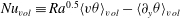 $Nu_{vol}\equiv Ra^{0.5}\langle v\unicode[STIX]{x1D703}\rangle _{vol}-\langle \unicode[STIX]{x2202}_{y}\unicode[STIX]{x1D703}\rangle _{vol}$
. It is easily found that, for RB cells,
$Nu_{vol}\equiv Ra^{0.5}\langle v\unicode[STIX]{x1D703}\rangle _{vol}-\langle \unicode[STIX]{x2202}_{y}\unicode[STIX]{x1D703}\rangle _{vol}$
. It is easily found that, for RB cells,
 $\unicode[STIX]{x1D6F7}_{y}(t)=Nu_{vol}(t)-1$
. The second bulk term
$\unicode[STIX]{x1D6F7}_{y}(t)=Nu_{vol}(t)-1$
. The second bulk term
 $\unicode[STIX]{x1D716}(t)>0$
stands for the viscous dissipation rate. Finally one may write
$\unicode[STIX]{x1D716}(t)>0$
stands for the viscous dissipation rate. Finally one may write
 $$\begin{eqnarray}\frac{\text{d}E_{kin}}{\text{d}t}=Pr\,Ra^{-0.5}[Nu_{vol}-(\unicode[STIX]{x1D716}+1)].\end{eqnarray}$$
The potential energy
 $E_{pot}$
verifies instead the relation
$E_{pot}$
verifies instead the relation
 $$\begin{eqnarray}\frac{\text{d}E_{pot}}{\text{d}t}=Pr\,Ra^{-0.5}[-Nu_{vol}+\unicode[STIX]{x1D6F7}_{b1}],\end{eqnarray}$$
which contains the bulk term
 $Nu_{vol}$
and a boundary term
$Nu_{vol}$
and a boundary term
 $$\begin{eqnarray}\unicode[STIX]{x1D6F7}_{b1}(t)\equiv -\oint y[\boldsymbol{n}\boldsymbol{\cdot }\unicode[STIX]{x1D735}\unicode[STIX]{x1D703}]\,\text{d}l\end{eqnarray}$$
quantifying the conversion rate to
 $E_{pot}$
from external sources. More precisely, let us introduce the Nusselt number
$E_{pot}$
from external sources. More precisely, let us introduce the Nusselt number
 $Nu_{top}(t)\equiv -\int \unicode[STIX]{x2202}_{y}\unicode[STIX]{x1D703}\,\text{d}x$
evaluated at the top
$Nu_{top}(t)\equiv -\int \unicode[STIX]{x2202}_{y}\unicode[STIX]{x1D703}\,\text{d}x$
evaluated at the top
 $y=0.5$
as well as the Nusselt number
$y=0.5$
as well as the Nusselt number
 $Nu_{bot}(t)\equiv -\int \unicode[STIX]{x2202}_{y}\unicode[STIX]{x1D703}\,\text{d}x$
evaluated at the bottom plate
$Nu_{bot}(t)\equiv -\int \unicode[STIX]{x2202}_{y}\unicode[STIX]{x1D703}\,\text{d}x$
evaluated at the bottom plate
 $y=-0.5$
. For the present square cell, one easily verifies that
$y=-0.5$
. For the present square cell, one easily verifies that
 $\unicode[STIX]{x1D6F7}_{b1}=(Nu_{top}+Nu_{bot})/2$
and consequently
$\unicode[STIX]{x1D6F7}_{b1}=(Nu_{top}+Nu_{bot})/2$
and consequently
 $$\begin{eqnarray}\frac{\text{d}E_{pot}}{\text{d}t}=Pr\,Ra^{-0.5}\left[-Nu_{vol}+\frac{1}{2}(Nu_{top}+Nu_{bot})\right].\end{eqnarray}$$
Finally, the evolution equation for the available potential energy
 $E_{bpot}$
reads as
$E_{bpot}$
reads as
 $$\begin{eqnarray}\frac{\text{d}E_{bpot}}{\text{d}t}=Pr\,Ra^{-0.5}[\unicode[STIX]{x1D6F7}_{d}-\unicode[STIX]{x1D6F7}_{b2}],\quad \left\{\begin{array}{@{}rcl@{}}\!\unicode[STIX]{x1D6F7}_{d}\ & \equiv \ & \displaystyle \left\langle \frac{\unicode[STIX]{x2202}y_{r}}{\unicode[STIX]{x2202}\unicode[STIX]{x1D703}}\unicode[STIX]{x1D735}\unicode[STIX]{x1D703}\boldsymbol{\cdot }\unicode[STIX]{x1D735}\unicode[STIX]{x1D703}\right\rangle _{vol}=\langle \unicode[STIX]{x1D735}y_{r}\boldsymbol{\cdot }\unicode[STIX]{x1D735}\unicode[STIX]{x1D703}\rangle _{vol}\\ \!\unicode[STIX]{x1D6F7}_{b2}\ & \equiv \ & \displaystyle \oint y_{r}[\boldsymbol{n}\boldsymbol{\cdot }\unicode[STIX]{x1D735}\unicode[STIX]{x1D703}]\,\text{d}l,\end{array}\right.\end{eqnarray}$$
where the bulk term
 $\unicode[STIX]{x1D6F7}_{d}(t)$
quantifies the energy conversion rate due to diapycnal mixing. Since by definition
$\unicode[STIX]{x1D6F7}_{d}(t)$
quantifies the energy conversion rate due to diapycnal mixing. Since by definition
 $\unicode[STIX]{x2202}y_{r}/\unicode[STIX]{x2202}\unicode[STIX]{x1D703}>0$
,
$\unicode[STIX]{x2202}y_{r}/\unicode[STIX]{x2202}\unicode[STIX]{x1D703}>0$
,
 $\unicode[STIX]{x1D6F7}_{d}(t)$
is bound to be positive. The boundary term
$\unicode[STIX]{x1D6F7}_{d}(t)$
is bound to be positive. The boundary term
 $\unicode[STIX]{x1D6F7}_{b2}$
provides the conversion rate from external sources. For the present RB cells, since
$\unicode[STIX]{x1D6F7}_{b2}$
provides the conversion rate from external sources. For the present RB cells, since
 $y_{r}(x,1/2,t)=-1/2$
and
$y_{r}(x,1/2,t)=-1/2$
and
 $y_{r}(x,-1/2,t)=1/2$
and because adiabaticity of side walls it is clear that
$y_{r}(x,-1/2,t)=1/2$
and because adiabaticity of side walls it is clear that
 $\unicode[STIX]{x1D6F7}_{b2}(t)=\unicode[STIX]{x1D6F7}_{b1}(t)$
. Finally by subtracting (2.9) by (2.12), one gets
$\unicode[STIX]{x1D6F7}_{b2}(t)=\unicode[STIX]{x1D6F7}_{b1}(t)$
. Finally by subtracting (2.9) by (2.12), one gets
 $$\begin{eqnarray}\frac{\text{d}E_{apot}}{\text{d}t}=Pr\,Ra^{-0.5}[Nu_{bot}+Nu_{top}-Nu_{vol}-\unicode[STIX]{x1D6F7}_{d}].\end{eqnarray}$$
3 Numerical method
Simulations are carried out using a finite volume code using a semi-implicit scheme based on the Bell–Colella–Glaz advection scheme (Bell, Colella & Glaz Reference Bell, Colella and Glaz1989), and a pressure-correction scheme for the velocity–pressure coupling, with a global second-order precision. Numerical implementation is done using BASILISK C, details of which can be found in Popinet (Reference Popinet2016). Simulations listed in table 1 have been performed on a uniform Cartesian grid with 512 points in each direction, with a variable time step that verifies the Courant–Friedrichs–Lewy condition CFL
 ${<}$
0.5. In the most unfavourable case (
${<}$
0.5. In the most unfavourable case (
 $Ra=10^{8},Pr=4.3$
) the thermal boundary layers contain 10 points along the vertical direction.
$Ra=10^{8},Pr=4.3$
) the thermal boundary layers contain 10 points along the vertical direction.
Spatial resolution is verified evaluating numerical convergence of time-averaged Nusselt numbers obtained by different methods (Stevens, Verzicco & Lohse Reference Stevens, Verzicco and Lohse2010). Note that to perform the averaging, statistical sampling is obtained at regular intervals. We compare
 $\overline{Nu}_{vol}$
,
$\overline{Nu}_{vol}$
,
 $\overline{Nu}_{top}$
and
$\overline{Nu}_{top}$
and
 $\overline{Nu}_{bot}$
to the Nusselt numbers obtained from the thermal and viscous dissipations
$\overline{Nu}_{bot}$
to the Nusselt numbers obtained from the thermal and viscous dissipations
 $$\begin{eqnarray}\overline{Nu}_{\unicode[STIX]{x1D703}}\equiv \langle \overline{\unicode[STIX]{x1D735}\unicode[STIX]{x1D703}\boldsymbol{\cdot }\unicode[STIX]{x1D735}\unicode[STIX]{x1D703}}\rangle _{vol},\quad \overline{Nu}_{\unicode[STIX]{x1D716}}\equiv \overline{\unicode[STIX]{x1D716}}+1.\end{eqnarray}$$
All these quantities should be equal (Shraiman & Siggia Reference Shraiman and Siggia1990). The value of
 $\overline{Nu}$
shown in table 1 is the average value of
$\overline{Nu}$
shown in table 1 is the average value of
 $\overline{Nu}_{vol}$
,
$\overline{Nu}_{vol}$
,
 $\overline{Nu}_{top}$
,
$\overline{Nu}_{top}$
,
 $\overline{Nu}_{bot}$
,
$\overline{Nu}_{bot}$
,
 $\overline{Nu}_{\unicode[STIX]{x1D703}}$
,
$\overline{Nu}_{\unicode[STIX]{x1D703}}$
,
 $\overline{Nu}_{\unicode[STIX]{x1D716}}$
while the maximum relative difference between any of them is shown as %Diff. These values converge within 2 % of
$\overline{Nu}_{\unicode[STIX]{x1D716}}$
while the maximum relative difference between any of them is shown as %Diff. These values converge within 2 % of
 $\overline{Nu}$
for all
$\overline{Nu}$
for all
 $(Ra,Pr)$
presented. We have also verified that our numerical results are well converged in a completely different way. This check has been performed by comparing results of the PDF of the time interval
$(Ra,Pr)$
presented. We have also verified that our numerical results are well converged in a completely different way. This check has been performed by comparing results of the PDF of the time interval
 $\unicode[STIX]{x1D70F}_{1}$
obtained by our code against benchmark results. This computation requires to get long-term simulations and was done for
$\unicode[STIX]{x1D70F}_{1}$
obtained by our code against benchmark results. This computation requires to get long-term simulations and was done for
 $(Ra=5\times 10^{7},Pr=4.3)$
since such parameter values had already been computed by a spectral code (Podvin & Sergent Reference Podvin and Sergent2015). The data for this check are postponed to the end of § 4.
$(Ra=5\times 10^{7},Pr=4.3)$
since such parameter values had already been computed by a spectral code (Podvin & Sergent Reference Podvin and Sergent2015). The data for this check are postponed to the end of § 4.
Table 1. For various Prandtl and Rayleigh numbers, the table provides the simulation length in convective time units, the number of reversal events, the average Nusselt number and maximum relative difference between
 $\overline{Nu}_{vol}$
,
$\overline{Nu}_{vol}$
,
 $\overline{Nu}_{top}$
,
$\overline{Nu}_{top}$
,
 $\overline{Nu}_{bot}$
,
$\overline{Nu}_{bot}$
,
 $\overline{Nu}_{\unicode[STIX]{x1D703}}$
, and
$\overline{Nu}_{\unicode[STIX]{x1D703}}$
, and
 $\overline{Nu}_{\unicode[STIX]{x1D716}}$
.
$\overline{Nu}_{\unicode[STIX]{x1D716}}$
.

4 Temporal analysis and statistical characterisation
In the present work, we focus on turbulent RB systems for which flow reversals are observed. For
 $Pr=3.0$
, this dynamics is associated with the interval
$Pr=3.0$
, this dynamics is associated with the interval
 $Ra\in [5\times 10^{6},3\times 10^{8}]$
. For
$Ra\in [5\times 10^{6},3\times 10^{8}]$
. For
 $Pr=4.3$
, it corresponds to the interval
$Pr=4.3$
, it corresponds to the interval
 $Ra\in [3\times 10^{7},4\times 10^{8}]$
(Sugiyama et al.
Reference Sugiyama, Ni, Stevens, Chan, Zhou, Xi, Sun, Grossmann, Xia and Lohse2010). Note that, these boundaries are not clearly established. For instance, some transitions were found for very long runs at
$Ra\in [3\times 10^{7},4\times 10^{8}]$
(Sugiyama et al.
Reference Sugiyama, Ni, Stevens, Chan, Zhou, Xi, Sun, Grossmann, Xia and Lohse2010). Note that, these boundaries are not clearly established. For instance, some transitions were found for very long runs at
 $(Pr=4.3,Ra=10^{7})$
(not presented here) but it is difficult to assert whether or not the few cycles observed correspond to an established statistical steady state or to a transient behaviour. In the following, we consider only values inside the aforementioned range for which the number of events is large enough (see table 1): simulations are performed from 9600 to 29 000 convective time units (see table 1), which gives from 50 to 160 events (except for
$(Pr=4.3,Ra=10^{7})$
(not presented here) but it is difficult to assert whether or not the few cycles observed correspond to an established statistical steady state or to a transient behaviour. In the following, we consider only values inside the aforementioned range for which the number of events is large enough (see table 1): simulations are performed from 9600 to 29 000 convective time units (see table 1), which gives from 50 to 160 events (except for
 $Pr=4.3$
and
$Pr=4.3$
and
 $Ra=3\times 10^{7}$
which is situated close to the boundary region where the reversal dynamics is established).
$Ra=3\times 10^{7}$
which is situated close to the boundary region where the reversal dynamics is established).
For a given couple
 $(Ra,Pr)$
, one computes the percentage of time, or equivalently the probability, that the system be in one of the three states:
$(Ra,Pr)$
, one computes the percentage of time, or equivalently the probability, that the system be in one of the three states:
 $p_{cr}$
in the CR regime,
$p_{cr}$
in the CR regime,
 $p_{ec}$
in the EC regime and
$p_{ec}$
in the EC regime and
 $p_{rr}$
inside a ‘rogue’ reversal. The probability
$p_{rr}$
inside a ‘rogue’ reversal. The probability
 $p_{rr}$
of rogue events is always of a few per cent (see table 2). For both
$p_{rr}$
of rogue events is always of a few per cent (see table 2). For both
 $Pr=3.0$
and
$Pr=3.0$
and
 $Pr=4.3$
, in the interval where the CR regime is observed,
$Pr=4.3$
, in the interval where the CR regime is observed,
 $p_{cr}$
first decreases and then increases with increasing
$p_{cr}$
first decreases and then increases with increasing
 $Ra$
(see table 2).
$Ra$
(see table 2).

Figure 3. PDF of
 $\unicode[STIX]{x1D70F}_{1}$
(a,b) and
$\unicode[STIX]{x1D70F}_{1}$
(a,b) and
 $\unicode[STIX]{x1D70F}_{d}$
(c,d) for
$\unicode[STIX]{x1D70F}_{d}$
(c,d) for
 $Pr=4.3$
, (a,c)
$Pr=4.3$
, (a,c)
 $Ra=5\times 10^{7}$
, (b,d)
$Ra=5\times 10^{7}$
, (b,d)
 $Ra=10^{8}$
. The PDF value is represented by ○ marks. For
$Ra=10^{8}$
. The PDF value is represented by ○ marks. For
 $\unicode[STIX]{x1D70F}_{1}$
it is the sum of three conditional PDFs: one shown by a thick blue line corresponding to the CR regime, a smaller one shown by an intermediate violet line corresponding to ‘rogue reversals’ and an additional part shown by a fine red line corresponding to the EC regime.
$\unicode[STIX]{x1D70F}_{1}$
it is the sum of three conditional PDFs: one shown by a thick blue line corresponding to the CR regime, a smaller one shown by an intermediate violet line corresponding to ‘rogue reversals’ and an additional part shown by a fine red line corresponding to the EC regime.
Table 2. Probabilities as a function of
 $Ra$
and
$Ra$
and
 $Pr$
.
$Pr$
.
 $p_{cr}$
(respectively
$p_{cr}$
(respectively
 $p_{ec}$
) denotes the probability that the system be inside the CR (respectively EC) regime.
$p_{ec}$
) denotes the probability that the system be inside the CR (respectively EC) regime.
 $p_{rr}$
denotes the probability of a ‘rogue’ reversal.
$p_{rr}$
denotes the probability of a ‘rogue’ reversal.

The PDFs of
 $\unicode[STIX]{x1D70F}_{1}$
and
$\unicode[STIX]{x1D70F}_{1}$
and
 $\unicode[STIX]{x1D70F}_{d}$
are measured based on the full simulation length and shown in figure 3 (respectively figure 4) for
$\unicode[STIX]{x1D70F}_{d}$
are measured based on the full simulation length and shown in figure 3 (respectively figure 4) for
 $Pr=4.3$
(respectively
$Pr=4.3$
(respectively
 $Pr=3$
). Using the filtering method of § 2.1, we separated the PDF of
$Pr=3$
). Using the filtering method of § 2.1, we separated the PDF of
 $\unicode[STIX]{x1D70F}_{1}$
into three contributions: one for intervals inside the CR regime (colour blue), one for intervals from the EC regime (colour red) and one corresponding to rogue events (colour purple). This PDF shows that the distribution of
$\unicode[STIX]{x1D70F}_{1}$
into three contributions: one for intervals inside the CR regime (colour blue), one for intervals from the EC regime (colour red) and one corresponding to rogue events (colour purple). This PDF shows that the distribution of
 $\unicode[STIX]{x1D70F}_{1}$
is not peaked inside the CR regime: intervals may have different durations. This is also valid for the EC regime. For
$\unicode[STIX]{x1D70F}_{1}$
is not peaked inside the CR regime: intervals may have different durations. This is also valid for the EC regime. For
 $Pr=4.3$
, a similar probability distribution of
$Pr=4.3$
, a similar probability distribution of
 $\unicode[STIX]{x1D70F}_{1}$
is observed for both values of
$\unicode[STIX]{x1D70F}_{1}$
is observed for both values of
 $Ra$
(figure 3) and a characteristic time scale
$Ra$
(figure 3) and a characteristic time scale
 $\unicode[STIX]{x1D70F}_{c}\approx 60$
exists which separates the EC and CR regimes. For
$\unicode[STIX]{x1D70F}_{c}\approx 60$
exists which separates the EC and CR regimes. For
 $Pr=3.0$
, a change in the PDFs of
$Pr=3.0$
, a change in the PDFs of
 $\unicode[STIX]{x1D70F}_{1}$
and
$\unicode[STIX]{x1D70F}_{1}$
and
 $\unicode[STIX]{x1D70F}_{d}$
is observed as we increase the values of
$\unicode[STIX]{x1D70F}_{d}$
is observed as we increase the values of
 $Ra$
(figure 4). For the lowest
$Ra$
(figure 4). For the lowest
 $Ra$
displayed, a characteristic time
$Ra$
displayed, a characteristic time
 $\unicode[STIX]{x1D70F}_{c}$
cannot be clearly defined. For the highest
$\unicode[STIX]{x1D70F}_{c}$
cannot be clearly defined. For the highest
 $Ra$
displayed
$Ra$
displayed
 $Ra=10^{8}$
, the EC regime completely disappears. For intermediate
$Ra=10^{8}$
, the EC regime completely disappears. For intermediate
 $Ra$
, reversal events become evenly distributed over a narrow band of
$Ra$
, reversal events become evenly distributed over a narrow band of
 $\unicode[STIX]{x1D70F}_{1}$
(see figure 4
b,e and c,f) and a clear separation of time scales between the EC and CR regimes is observed at
$\unicode[STIX]{x1D70F}_{1}$
(see figure 4
b,e and c,f) and a clear separation of time scales between the EC and CR regimes is observed at
 $\unicode[STIX]{x1D70F}_{c}\approx 50$
which is at least one order of magnitude larger than the large eddy turnover time,
$\unicode[STIX]{x1D70F}_{c}\approx 50$
which is at least one order of magnitude larger than the large eddy turnover time,
 $\unicode[STIX]{x1D70F}_{E}\equiv 4\unicode[STIX]{x03C0}/\overline{|\unicode[STIX]{x1D714}_{c}|}$
(
$\unicode[STIX]{x1D70F}_{E}\equiv 4\unicode[STIX]{x03C0}/\overline{|\unicode[STIX]{x1D714}_{c}|}$
(
 $\unicode[STIX]{x1D714}_{c}$
denoting vorticity measured at the cavity centre). The PDF of the inter-switch intervals observed for cylindrical convection cell experiments is an exponential distribution (Sreenivasan et al.
Reference Sreenivasan, Bershadskii and Niemela2002). It is not seen here (figures 3 and 4) illustrating the fact that rotation-led reversals are not present here contrary to cylindrical cells.
$\unicode[STIX]{x1D714}_{c}$
denoting vorticity measured at the cavity centre). The PDF of the inter-switch intervals observed for cylindrical convection cell experiments is an exponential distribution (Sreenivasan et al.
Reference Sreenivasan, Bershadskii and Niemela2002). It is not seen here (figures 3 and 4) illustrating the fact that rotation-led reversals are not present here contrary to cylindrical cells.

Figure 4. PDF for
 $\unicode[STIX]{x1D70F}_{1}$
(a–c) and
$\unicode[STIX]{x1D70F}_{1}$
(a–c) and
 $\unicode[STIX]{x1D70F}_{d}$
(d–f) for
$\unicode[STIX]{x1D70F}_{d}$
(d–f) for
 $Pr=3.0$
and
$Pr=3.0$
and
 $Ra=10^{7}$
(a,d),
$Ra=10^{7}$
(a,d),
 $Ra=5\times 10^{7}$
(b,e) and
$Ra=5\times 10^{7}$
(b,e) and
 $Ra=10^{8}$
(c,f). Layout is similar to figure 4.
$Ra=10^{8}$
(c,f). Layout is similar to figure 4.
From the PDF of transition durations,
 $\unicode[STIX]{x1D70F}_{d}$
, for the CR regime only (see figures 3
c,d and 4
d–f), the peak value tends to increase as
$\unicode[STIX]{x1D70F}_{d}$
, for the CR regime only (see figures 3
c,d and 4
d–f), the peak value tends to increase as
 $Ra$
is increased for both
$Ra$
is increased for both
 $Pr=3.0$
and
$Pr=3.0$
and
 $Pr=4.3$
. Concerning the numerical check, the average value
$Pr=4.3$
. Concerning the numerical check, the average value
 $\overline{\unicode[STIX]{x1D70F}_{1}}|_{cr}$
during the CR regime and the average duration
$\overline{\unicode[STIX]{x1D70F}_{1}}|_{cr}$
during the CR regime and the average duration
 $\overline{\unicode[STIX]{x1D70F}_{d}}$
of transition were both found to be in good agreement with published results for
$\overline{\unicode[STIX]{x1D70F}_{d}}$
of transition were both found to be in good agreement with published results for
 $(Ra=5\times 10^{7},Pr=4.3)$
:
$(Ra=5\times 10^{7},Pr=4.3)$
:
 $\overline{\unicode[STIX]{x1D70F}_{1}}|_{cr}=146$
and
$\overline{\unicode[STIX]{x1D70F}_{1}}|_{cr}=146$
and
 $\overline{\unicode[STIX]{x1D70F}_{d}}=11.5$
convective time units (Podvin & Sergent Reference Podvin and Sergent2015).
$\overline{\unicode[STIX]{x1D70F}_{d}}=11.5$
convective time units (Podvin & Sergent Reference Podvin and Sergent2015).
5 Dynamics of the generic reversal
We have shown above that reversals cycles have different durations
 $\unicode[STIX]{x1D70F}_{1,i}$
. A simple time rescaling, however, can be used to identify features common to all reversal cycles.
$\unicode[STIX]{x1D70F}_{1,i}$
. A simple time rescaling, however, can be used to identify features common to all reversal cycles.
5.1 Averaging procedure and generic reversal as function of
 $(Ra,Pr)$


Figure 5. From (a) to (i): normalised global angular impulse
 $L_{2D}/\overline{|L_{2D}|}$
, normalised kinetic energy
$L_{2D}/\overline{|L_{2D}|}$
, normalised kinetic energy
 $E_{kin}/\overline{|E_{kin}|}$
and normalised available potential energy
$E_{kin}/\overline{|E_{kin}|}$
and normalised available potential energy
 $E_{apot}/\overline{|E_{kin}|}$
for
$E_{apot}/\overline{|E_{kin}|}$
for
 $(Ra=5\times 10^{7},Pr=4.3)$
. (a,d,g) Each reversal cycle is centred and its time is rescaled by
$(Ra=5\times 10^{7},Pr=4.3)$
. (a,d,g) Each reversal cycle is centred and its time is rescaled by
 $\overline{\unicode[STIX]{x1D70F}}_{1}$
(only
$\overline{\unicode[STIX]{x1D70F}}_{1}$
(only
 $10$
reversals are displayed and each colour is a different reversal); (b,e,h) each reversal cycle is centred and its time is rescaled by
$10$
reversals are displayed and each colour is a different reversal); (b,e,h) each reversal cycle is centred and its time is rescaled by
 $\unicode[STIX]{x1D70F}_{1,i}$
; (c,f,i) average value of rescaled curves obtained from the complete time series (thick lines) and curves corresponding to one standard deviation (dashed lines).
$\unicode[STIX]{x1D70F}_{1,i}$
; (c,f,i) average value of rescaled curves obtained from the complete time series (thick lines) and curves corresponding to one standard deviation (dashed lines).
In order to identify similarities between different intervals in the CR regime, the following procedure is proposed to treat time series of global quantities such as
 $L_{2D}$
,
$L_{2D}$
,
 $E_{kin}$
and
$E_{kin}$
and
 $E_{apot}$
. Once the intervals
$E_{apot}$
. Once the intervals
 $[r_{i},r_{i+1}]$
inside the CR regime are properly identified, all these intervals with
$[r_{i},r_{i+1}]$
inside the CR regime are properly identified, all these intervals with
 $L_{2D}>0$
(respectively
$L_{2D}>0$
(respectively
 $L_{2D}<0$
) are stacked together so that they have a common origin at
$L_{2D}<0$
) are stacked together so that they have a common origin at
 $r_{i}$
(respectively
$r_{i}$
(respectively
 $r_{i+1}$
). If the time axis of each interval is rescaled by
$r_{i+1}$
). If the time axis of each interval is rescaled by
 $\overline{\unicode[STIX]{x1D70F}_{1}}$
, one obtains figure 5(a,d,g). If the time axis of each interval is rescaled by its particular duration
$\overline{\unicode[STIX]{x1D70F}_{1}}$
, one obtains figure 5(a,d,g). If the time axis of each interval is rescaled by its particular duration
 $\unicode[STIX]{x1D70F}_{1,i}$
, these curves display a consistent dynamical pattern (see figure 5
b,e,h). Note that, while figure 5 displays only 10 reversals to avoid cluttered graphs, these events displayed are considered as representative of the entire set. Obviously, all of the events inside the CR regime are taken into account in our procedure but ‘rogue reversal’ events are not. This procedure is similar to one used in the study of statistical properties of magnetic switches in the geodynamo problem (Valet et al.
Reference Valet, Fournier, Courtillot and Herrero-Bervera2012; Lhuillier et al.
Reference Lhuillier, Hulot and Gallet2013). For a sufficiently large number of recorded events, the average over these rescaled curves is expected to remove the noisy dynamics and to represent a generic reversal cycle (figure 5
c,f,i). This averaging technique, once applied to
$\unicode[STIX]{x1D70F}_{1,i}$
, these curves display a consistent dynamical pattern (see figure 5
b,e,h). Note that, while figure 5 displays only 10 reversals to avoid cluttered graphs, these events displayed are considered as representative of the entire set. Obviously, all of the events inside the CR regime are taken into account in our procedure but ‘rogue reversal’ events are not. This procedure is similar to one used in the study of statistical properties of magnetic switches in the geodynamo problem (Valet et al.
Reference Valet, Fournier, Courtillot and Herrero-Bervera2012; Lhuillier et al.
Reference Lhuillier, Hulot and Gallet2013). For a sufficiently large number of recorded events, the average over these rescaled curves is expected to remove the noisy dynamics and to represent a generic reversal cycle (figure 5
c,f,i). This averaging technique, once applied to
 $E_{kin}$
and
$E_{kin}$
and
 $E_{apot}$
, recovers the evolution of mechanical energies during the generic reversal cycle.
$E_{apot}$
, recovers the evolution of mechanical energies during the generic reversal cycle.

Figure 6. Curves corresponding to reversals for
 $Pr=3.0$
as obtained using the procedure described in figure 5. The average
$Pr=3.0$
as obtained using the procedure described in figure 5. The average
 $L_{2D}/\overline{|L_{2D}|}$
is shown in thick lines and one standard deviation in dashed lines. From (a) to (c): (
$L_{2D}/\overline{|L_{2D}|}$
is shown in thick lines and one standard deviation in dashed lines. From (a) to (c): (
 $a$
)
$a$
)
 $Ra=10^{7}$
, (
$Ra=10^{7}$
, (
 $b$
)
$b$
)
 $Ra=5\times 10^{7}$
and (
$Ra=5\times 10^{7}$
and (
 $c$
)
$c$
)
 $Ra=10^{8}$
.
$Ra=10^{8}$
.

Figure 7. Conditionally averaged fields
 $\boldsymbol{u}^{o}(x,y,t)$
and
$\boldsymbol{u}^{o}(x,y,t)$
and
 $y_{r}(\unicode[STIX]{x1D703}^{o}(x,y,t))$
at different instants during the generic reversal cycle for
$y_{r}(\unicode[STIX]{x1D703}^{o}(x,y,t))$
at different instants during the generic reversal cycle for
 $(Ra=5\times 10^{7},Pr=3.0)$
. Fields are obtained as the ensemble average over 83 particular reversal cycles. Streamlines of the velocity field
$(Ra=5\times 10^{7},Pr=3.0)$
. Fields are obtained as the ensemble average over 83 particular reversal cycles. Streamlines of the velocity field
 $\boldsymbol{u}^{o}$
are superposed over the colour map of field
$\boldsymbol{u}^{o}$
are superposed over the colour map of field
 $y_{r}(\unicode[STIX]{x1D703}^{o})$
. Solid and dashed streamlines indicate the two senses of rotation.
$y_{r}(\unicode[STIX]{x1D703}^{o})$
. Solid and dashed streamlines indicate the two senses of rotation.
Figure 6 shows the
 $L_{2D}/\overline{|L_{2D}|}$
curves for generic reversal cycle at
$L_{2D}/\overline{|L_{2D}|}$
curves for generic reversal cycle at
 $Pr=3.0$
: as we increase
$Pr=3.0$
: as we increase
 $Ra$
, the reversal cycle becomes more regular and the band representing the standard deviation narrows. The same averaging procedure can be applied to instantaneous temperature and velocity fields in order to obtain the evolution of a conditionally averaged temperature
$Ra$
, the reversal cycle becomes more regular and the band representing the standard deviation narrows. The same averaging procedure can be applied to instantaneous temperature and velocity fields in order to obtain the evolution of a conditionally averaged temperature
 $\unicode[STIX]{x1D703}^{o}(x,y,t)$
and velocity
$\unicode[STIX]{x1D703}^{o}(x,y,t)$
and velocity
 $\boldsymbol{u}^{o}(x,y,t)$
fields during the reversal cycle (e.g. figure 7 for
$\boldsymbol{u}^{o}(x,y,t)$
fields during the reversal cycle (e.g. figure 7 for
 $(Ra=5\times 10^{7},Pr=3.0)$
). Despite fluctuations between various realisations, dominant and persistent structures appear at specific times of the generic cycle.
$(Ra=5\times 10^{7},Pr=3.0)$
). Despite fluctuations between various realisations, dominant and persistent structures appear at specific times of the generic cycle.
5.2 Phases of reversal cycle

Figure 8. Generic reversal cycle for
 $(Ra=5\times 10^{7},Pr=3.0)$
. (a) System trajectory in phase space
$(Ra=5\times 10^{7},Pr=3.0)$
. (a) System trajectory in phase space
 $(L_{2D}/\overline{|L_{2D}|},E_{kin}/\overline{|E_{kin}|},E_{apot}/\overline{|E_{kin}|})$
; (b–d) average curves for
$(L_{2D}/\overline{|L_{2D}|},E_{kin}/\overline{|E_{kin}|},E_{apot}/\overline{|E_{kin}|})$
; (b–d) average curves for
 $L_{2D}/\overline{|L_{2D}|}$
,
$L_{2D}/\overline{|L_{2D}|}$
,
 $E_{kin}/\overline{|E_{kin}|}$
and
$E_{kin}/\overline{|E_{kin}|}$
and
 $E_{apot}/\overline{|E_{kin}|}$
. Marks (i)–(x) and (a)–(e) indicate particular instants (see text for explanations). The accumulation phase is shaded and indicated by a blue colour bar. The release (respectively acceleration) phase is indicated by an orange (respectively green) colour bar. The same colour code is used in the phase space trajectory position.
$E_{apot}/\overline{|E_{kin}|}$
. Marks (i)–(x) and (a)–(e) indicate particular instants (see text for explanations). The accumulation phase is shaded and indicated by a blue colour bar. The release (respectively acceleration) phase is indicated by an orange (respectively green) colour bar. The same colour code is used in the phase space trajectory position.
In the phase space
 $(L_{2D}/\overline{|L_{2D}|},E_{kin}/\overline{|E_{kin}|},E_{apot}/\overline{|E_{kin}|})$
, let us consider the generic reversal cycle (figure 8). Consecutive instants (a)–(e) pinpoints particular dynamical times:
$(L_{2D}/\overline{|L_{2D}|},E_{kin}/\overline{|E_{kin}|},E_{apot}/\overline{|E_{kin}|})$
, let us consider the generic reversal cycle (figure 8). Consecutive instants (a)–(e) pinpoints particular dynamical times:
 $L_{2D}=0$
at instant (a);
$L_{2D}=0$
at instant (a);
 $E_{kin}$
reaches a local maximum at instant (b),
$E_{kin}$
reaches a local maximum at instant (b),
 $E_{kin}$
reaches a local minimum at instant (c);
$E_{kin}$
reaches a local minimum at instant (c);
 $E_{apot}$
reaches its minimum at instant (d);
$E_{apot}$
reaches its minimum at instant (d);
 $|L_{2D}|$
reaches its maximum at instant (e). Points (
$|L_{2D}|$
reaches its maximum at instant (e). Points (
 $\text{a}^{\prime }$
)–(
$\text{a}^{\prime }$
)–(
 $\text{e}^{\prime }$
) are similar but correspond to an opposite rotation sign. Based on these instants, three successive phases are identified for the generic reversal cycle. They are called accumulation, release and acceleration.
$\text{e}^{\prime }$
) are similar but correspond to an opposite rotation sign. Based on these instants, three successive phases are identified for the generic reversal cycle. They are called accumulation, release and acceleration.

Figure 9. (a,b) Generic reversal curves in the plane (
 $L_{2D}/\overline{|L_{2D}|}$
,
$L_{2D}/\overline{|L_{2D}|}$
,
 $E_{kin}/\overline{|E_{kin}|}$
). Each curve corresponds to a different
$E_{kin}/\overline{|E_{kin}|}$
). Each curve corresponds to a different
 $Ra$
:
$Ra$
:
 $Ra=3\times 10^{7}$
(black line),
$Ra=3\times 10^{7}$
(black line),
 $Ra=5\times 10^{7}$
(blue line) and
$Ra=5\times 10^{7}$
(blue line) and
 $Ra=10^{8}$
(red line). (a) Corresponds to
$Ra=10^{8}$
(red line). (a) Corresponds to
 $Pr=3.0$
and (b) to
$Pr=3.0$
and (b) to
 $Pr=4.3$
. (c–e) Average curves during one cycle for
$Pr=4.3$
. (c–e) Average curves during one cycle for
 $L_{2D}/\overline{|L_{2D}|}$
,
$L_{2D}/\overline{|L_{2D}|}$
,
 $E_{kin}/\overline{|E_{kin}|}$
and
$E_{kin}/\overline{|E_{kin}|}$
and
 $E_{apot}/\overline{|E_{kin}|}$
for
$E_{apot}/\overline{|E_{kin}|}$
for
 $(Ra=5\times 10^{7},Pr=4.3)$
. Figures are displayed as in figure 8.
$(Ra=5\times 10^{7},Pr=4.3)$
. Figures are displayed as in figure 8.
The accumulation phase is located between points (
 $\text{e}^{\prime }$
) and (a). It is characterised by a steady accumulation of
$\text{e}^{\prime }$
) and (a). It is characterised by a steady accumulation of
 $E_{apot}$
and a progressive decay of
$E_{apot}$
and a progressive decay of
 $|L_{2D}|$
and
$|L_{2D}|$
and
 $E_{kin}$
. This phase ends when
$E_{kin}$
. This phase ends when
 $E_{apot}$
reaches a maximum and
$E_{apot}$
reaches a maximum and
 $E_{kin}$
a minimum (figure 8). In terms of generic velocity field
$E_{kin}$
a minimum (figure 8). In terms of generic velocity field
 $\boldsymbol{u}^{o}(x,y,t)$
, a central vortex is present during this phase (see figure 7i–iii) until the global rotation switches signs at point (a) i.e.
$\boldsymbol{u}^{o}(x,y,t)$
, a central vortex is present during this phase (see figure 7i–iii) until the global rotation switches signs at point (a) i.e.
 $L_{2D}=0$
(figure 7iv).
$L_{2D}=0$
(figure 7iv).
The release phase located between points (a) and (d), is defined by a sudden exchange from
 $E_{apot}$
to
$E_{apot}$
to
 $E_{kin}$
. It can be split in three substeps. The first step from point (a) to point (b) contains a rapid increase of
$E_{kin}$
. It can be split in three substeps. The first step from point (a) to point (b) contains a rapid increase of
 $E_{kin}$
to a maximum value and a rapid decrease of
$E_{kin}$
to a maximum value and a rapid decrease of
 $E_{apot}$
. It corresponds to figure 7(v–vii). A second step follows from points (b) to (c) in which
$E_{apot}$
. It corresponds to figure 7(v–vii). A second step follows from points (b) to (c) in which
 $E_{kin}$
suddenly decreases and
$E_{kin}$
suddenly decreases and
 $E_{apot}$
remains almost constant. This is associated with figure 7(viii,ix). After these two steps referred to as a rebound, a new increase of
$E_{apot}$
remains almost constant. This is associated with figure 7(viii,ix). After these two steps referred to as a rebound, a new increase of
 $E_{kin}$
is observed from points (c) to (d) concomitantly with a decrease of
$E_{kin}$
is observed from points (c) to (d) concomitantly with a decrease of
 $E_{apot}$
until it reaches its minimum value.
$E_{apot}$
until it reaches its minimum value.
Finally, the acceleration phase is located between points (d) and (e) and is characterised by an increase of
 $|L_{2D}|$
and
$|L_{2D}|$
and
 $E_{kin}$
to peak values, whereas
$E_{kin}$
to peak values, whereas
 $E_{apot}$
remains almost constant. During this period, the flow reorganises gradually into a single dominant vortex (figure 7x).
$E_{apot}$
remains almost constant. During this period, the flow reorganises gradually into a single dominant vortex (figure 7x).
For the
 $(Ra,Pr)$
considered inside the CR regime, we are able to recover a generic reversal cycle expressed in terms of the available mechanical energy (figure 9). Similarities between these curves for different
$(Ra,Pr)$
considered inside the CR regime, we are able to recover a generic reversal cycle expressed in terms of the available mechanical energy (figure 9). Similarities between these curves for different
 $(Ra,Pr)$
suggest an equivalent underlying mechanism behind flow reversals, even if the intensity of the rebound decreases with
$(Ra,Pr)$
suggest an equivalent underlying mechanism behind flow reversals, even if the intensity of the rebound decreases with
 $Pr$
. For
$Pr$
. For
 $(Ra=5\times 10^{7},Pr=3.0)$
, the accumulation phase lasts longer (60 %), while the release and acceleration phases have shorter and similar durations (respectively 18 % and 22 % of the reversal cycle). For the range of
$(Ra=5\times 10^{7},Pr=3.0)$
, the accumulation phase lasts longer (60 %), while the release and acceleration phases have shorter and similar durations (respectively 18 % and 22 % of the reversal cycle). For the range of
 $Ra$
considered these proportions are similar: for instance, the accumulation, release, and acceleration are observed to last 75, 13 and 12 % of the reversal cycle for
$Ra$
considered these proportions are similar: for instance, the accumulation, release, and acceleration are observed to last 75, 13 and 12 % of the reversal cycle for
 $(Ra=10^{8},Pr=3.0)$
.
$(Ra=10^{8},Pr=3.0)$
.
6 Dynamics of a particular reversal
From now on, we focus on a single value of
 $(Ra,Pr)$
 $(Ra=5\times 10^{7},Pr=3.0)$
in order to explore the nature of the reversal dynamics. To look at the small-scale effects, the analysis below considers particular realisations of reversal cycles rather than conditionally averaged fields.
$(Ra=5\times 10^{7},Pr=3.0)$
in order to explore the nature of the reversal dynamics. To look at the small-scale effects, the analysis below considers particular realisations of reversal cycles rather than conditionally averaged fields.
For each particular reversal cycle, we define similarly to the generic curve, consecutive instants (
 $\text{a}_{p}$
)–(
$\text{a}_{p}$
)–(
 $\text{e}_{p}$
) which pinpoints the dynamical times:
$\text{e}_{p}$
) which pinpoints the dynamical times:
 $L_{2D}=0$
at instant (
$L_{2D}=0$
at instant (
 $\text{a}_{p}$
);
$\text{a}_{p}$
);
 $E_{kin}$
reaches a local maximum at instant (
$E_{kin}$
reaches a local maximum at instant (
 $\text{b}_{p}$
),
$\text{b}_{p}$
),
 $E_{kin}$
reaches a local minimum at instant (
$E_{kin}$
reaches a local minimum at instant (
 $\text{c}_{p}$
);
$\text{c}_{p}$
);
 $E_{apot}$
reaches its minimum at instant (
$E_{apot}$
reaches its minimum at instant (
 $\text{d}_{p}$
);
$\text{d}_{p}$
);
 $|L_{2D}|$
reaches its maximum at instant (
$|L_{2D}|$
reaches its maximum at instant (
 $\text{e}_{p}$
).
$\text{e}_{p}$
).
6.1 Time evolution of the available mechanical energy and flow structures

Figure 10. Instantaneous fields for a particular reversal cycle during the accumulation phase at regular time intervals at
 $(Ra=5\times 10^{7},Pr=3.0)$
. The first snapshot follows point (
$(Ra=5\times 10^{7},Pr=3.0)$
. The first snapshot follows point (
 $\text{e}_{p}^{\prime }$
) while the last precedes point (
$\text{e}_{p}^{\prime }$
) while the last precedes point (
 $\text{a}_{p}$
). Streamlines are superposed either to vorticity
$\text{a}_{p}$
). Streamlines are superposed either to vorticity
 $\unicode[STIX]{x1D714}$
(a), or to kinetic energy
$\unicode[STIX]{x1D714}$
(a), or to kinetic energy
 $1/2u_{i}u_{i}$
(b).
$1/2u_{i}u_{i}$
(b).

Figure 11. Instantaneous fields for a particular reversal cycle during the accumulation phase. They are identical to those of figure 10 but streamlines are superposed either to the field
 $Pr(y_{r}-y)\unicode[STIX]{x1D703}$
(a) or to the field
$Pr(y_{r}-y)\unicode[STIX]{x1D703}$
(a) or to the field
 $\unicode[STIX]{x1D735}y_{r}\boldsymbol{\cdot }\unicode[STIX]{x1D735}\unicode[STIX]{x1D703}$
(b). Snapshots correspond to the same instants as in figure 10.
$\unicode[STIX]{x1D735}y_{r}\boldsymbol{\cdot }\unicode[STIX]{x1D735}\unicode[STIX]{x1D703}$
(b). Snapshots correspond to the same instants as in figure 10.
The spatial distribution of mechanical energy can be linked to flow structures observed during different phases of a reversal cycle. At the beginning of the accumulation phase (point (
 $\text{e}_{p}^{\prime }$
)), a large diagonal vortex with small counter-rotating corner flows is observed (figure 10
a). On the one hand, it corresponds to a state of maximum kinetic energy condensed inside the central vortex (figure 10
b). On the other hand, the integrand
$\text{e}_{p}^{\prime }$
)), a large diagonal vortex with small counter-rotating corner flows is observed (figure 10
a). On the one hand, it corresponds to a state of maximum kinetic energy condensed inside the central vortex (figure 10
b). On the other hand, the integrand
 $Pr\int (y_{r}-y)$
of
$Pr\int (y_{r}-y)$
of
 $E_{apot}$
is mostly distributed inside the corner flows or along thin thermal boundary layers (figure 11
a). The field
$E_{apot}$
is mostly distributed inside the corner flows or along thin thermal boundary layers (figure 11
a). The field
 $\unicode[STIX]{x1D735}y_{r}\boldsymbol{\cdot }\unicode[STIX]{x1D735}\unicode[STIX]{x1D703}$
is used to highlight the contour of thermal plumes (figure 11
b). This field is related to the spatial distribution of
$\unicode[STIX]{x1D735}y_{r}\boldsymbol{\cdot }\unicode[STIX]{x1D735}\unicode[STIX]{x1D703}$
is used to highlight the contour of thermal plumes (figure 11
b). This field is related to the spatial distribution of
 $\unicode[STIX]{x1D6F7}_{d}$
(see (2.12)). Small-scale thermal plumes are observed to be detached from the thermal boundary layers. They are then swept by the central vortex. Plumes are channelled into the corner flows, directly or after having been advected along the side walls. The progressive growth of the corner flows is illustrated on figures 10 and 11. This is consistent with previous observations by Sugiyama et al. (Reference Sugiyama, Ni, Stevens, Chan, Zhou, Xi, Sun, Grossmann, Xia and Lohse2010) that tied the time evolution of the corner-flows heights. The steady increase in
$\unicode[STIX]{x1D6F7}_{d}$
(see (2.12)). Small-scale thermal plumes are observed to be detached from the thermal boundary layers. They are then swept by the central vortex. Plumes are channelled into the corner flows, directly or after having been advected along the side walls. The progressive growth of the corner flows is illustrated on figures 10 and 11. This is consistent with previous observations by Sugiyama et al. (Reference Sugiyama, Ni, Stevens, Chan, Zhou, Xi, Sun, Grossmann, Xia and Lohse2010) that tied the time evolution of the corner-flows heights. The steady increase in
 $E_{apot}$
coincides with a deceleration of the central vortex and to a build-up of thermal energy inside the corner flows. Indeed, let us compute the contributions to
$E_{apot}$
coincides with a deceleration of the central vortex and to a build-up of thermal energy inside the corner flows. Indeed, let us compute the contributions to
 $E_{apot}$
due to the region of thermal boundary layers (BL) and the bulk. The hot and cold BL are taken to have a constant thickness
$E_{apot}$
due to the region of thermal boundary layers (BL) and the bulk. The hot and cold BL are taken to have a constant thickness
 $\unicode[STIX]{x1D6FF}_{\unicode[STIX]{x1D703}}^{-1}=2\overline{Nu}$
. Contributions inside both BL (figure 12) amount to 30–40 % of
$\unicode[STIX]{x1D6FF}_{\unicode[STIX]{x1D703}}^{-1}=2\overline{Nu}$
. Contributions inside both BL (figure 12) amount to 30–40 % of
 $\overline{E_{apot}}$
and are fairly constant in time: standard deviation is less than 1 %. On the contrary, contributions to
$\overline{E_{apot}}$
and are fairly constant in time: standard deviation is less than 1 %. On the contrary, contributions to
 $E_{apot}$
from outside BL are directly influenced by the reversal cycle: a steady increase is observed during the accumulation phase until the release phase (figure 12). This suggests that the energy exchange observed during the release takes place only inside the bulk, while the boundary layers seem to be largely unaffected by the reversals.
$E_{apot}$
from outside BL are directly influenced by the reversal cycle: a steady increase is observed during the accumulation phase until the release phase (figure 12). This suggests that the energy exchange observed during the release takes place only inside the bulk, while the boundary layers seem to be largely unaffected by the reversals.

Figure 12. Evolution of
 $E_{apot}$
contained within the thermal boundary layers (blue line) and outside (black line) at
$E_{apot}$
contained within the thermal boundary layers (blue line) and outside (black line) at
 $(Ra=5\times 10^{7},Pr=3.0)$
.
$(Ra=5\times 10^{7},Pr=3.0)$
.

Figure 13. Instantaneous fields for a particular reversal cycle during the early release phase (point (
 $\text{a}_{p}$
)–(
$\text{a}_{p}$
)–(
 $\text{b}_{p}$
)) at regular time intervals
$\text{b}_{p}$
)) at regular time intervals
 $(Ra=5\times 10^{7},Pr=3.0)$
. Streamlines are superposed to the field
$(Ra=5\times 10^{7},Pr=3.0)$
. Streamlines are superposed to the field
 $1/2u_{i}u_{i}$
. First snapshot follows point (
$1/2u_{i}u_{i}$
. First snapshot follows point (
 $\text{a}_{p}$
), last precedes point (
$\text{a}_{p}$
), last precedes point (
 $\text{b}_{p}$
).
$\text{b}_{p}$
).

Figure 14. Instantaneous fields for a particular reversal cycle during the release phase at
 $(Ra=5\times 10^{7},Pr=3.0)$
. Snapshots correspond to points (
$(Ra=5\times 10^{7},Pr=3.0)$
. Snapshots correspond to points (
 $\text{a}_{p}$
) to (
$\text{a}_{p}$
) to (
 $\text{d}_{p}$
). Streamlines are superposed to either the field
$\text{d}_{p}$
). Streamlines are superposed to either the field
 $y_{r}(x,z,t)$
(a) or to field
$y_{r}(x,z,t)$
(a) or to field
 $\unicode[STIX]{x1D735}y_{r}\boldsymbol{\cdot }\unicode[STIX]{x1D735}\unicode[STIX]{x1D703}$
(b).
$\unicode[STIX]{x1D735}y_{r}\boldsymbol{\cdot }\unicode[STIX]{x1D735}\unicode[STIX]{x1D703}$
(b).
During the first part of the rebound (points (
 $\text{a}_{p}$
) to (
$\text{a}_{p}$
) to (
 $\text{b}_{p}$
)), the opposing corner flows have become large and strong enough to deform and finally split the central vortex (figure 13): opposing corner flows then connect and form a single vortex (with opposite rotation with respect to the previous LSC). This allows the thermal energy stored inside corners to be rapidly released and transformed into kinetic energy. By the end of this exchange, the amount of thermal energy
$\text{b}_{p}$
)), the opposing corner flows have become large and strong enough to deform and finally split the central vortex (figure 13): opposing corner flows then connect and form a single vortex (with opposite rotation with respect to the previous LSC). This allows the thermal energy stored inside corners to be rapidly released and transformed into kinetic energy. By the end of this exchange, the amount of thermal energy
 $E_{apot}$
stored outside the thermal boundary layers will be halved (figure 12). The complete rebound period (point (
$E_{apot}$
stored outside the thermal boundary layers will be halved (figure 12). The complete rebound period (point (
 $\text{a}_{p}$
)–(
$\text{a}_{p}$
)–(
 $\text{c}_{p}$
)) can be better illustrated by highlighting the role of the thermal plumes and boundary layers. To do so, one uses
$\text{c}_{p}$
)) can be better illustrated by highlighting the role of the thermal plumes and boundary layers. To do so, one uses
 $y_{r}(x,y,t)$
which is a bijective function of temperature, and function
$y_{r}(x,y,t)$
which is a bijective function of temperature, and function
 $\unicode[STIX]{x1D735}y_{r}\boldsymbol{\cdot }\unicode[STIX]{x1D735}\unicode[STIX]{x1D703}$
in figure 14. Once the vortex reconnection has taken place, the blobs of hot (respectively cold) fluid which are now inside the main central vortex, are allowed to travel upwards (respectively downwards) directly into the bulk. This results in the exchange of potential energy (contained inside small-scale structures) into kinetic energy (contained inside the central vortex). The newly formed circulation proceeds to rotate and is able to advect thermal blobs against the action of buoyancy forces (as seen between points (
$\unicode[STIX]{x1D735}y_{r}\boldsymbol{\cdot }\unicode[STIX]{x1D735}\unicode[STIX]{x1D703}$
in figure 14. Once the vortex reconnection has taken place, the blobs of hot (respectively cold) fluid which are now inside the main central vortex, are allowed to travel upwards (respectively downwards) directly into the bulk. This results in the exchange of potential energy (contained inside small-scale structures) into kinetic energy (contained inside the central vortex). The newly formed circulation proceeds to rotate and is able to advect thermal blobs against the action of buoyancy forces (as seen between points (
 $\text{b}_{p}$
) and (
$\text{b}_{p}$
) and (
 $\text{c}_{p}$
) figure 14). Simultaneously as the thermals are released into the bulk, the surface separating hot and cold fluid increases which reinforces the mixing process (figure 14
b).
$\text{c}_{p}$
) figure 14). Simultaneously as the thermals are released into the bulk, the surface separating hot and cold fluid increases which reinforces the mixing process (figure 14
b).

Figure 15. Instantaneous fields for a particular reversal cycle taken at regular intervals during the acceleration phase at
 $(Ra=5\times 10^{7},Pr=3.0)$
. The first snapshot follows point (
$(Ra=5\times 10^{7},Pr=3.0)$
. The first snapshot follows point (
 $\text{d}_{p}$
); the last corresponds to point (
$\text{d}_{p}$
); the last corresponds to point (
 $\text{e}_{p}$
). Streamlines are superposed either to vorticity
$\text{e}_{p}$
). Streamlines are superposed either to vorticity
 $\unicode[STIX]{x1D714}$
(a), or to
$\unicode[STIX]{x1D714}$
(a), or to
 $\unicode[STIX]{x1D735}y_{r}\boldsymbol{\cdot }\unicode[STIX]{x1D735}\unicode[STIX]{x1D703}$
(b).
$\unicode[STIX]{x1D735}y_{r}\boldsymbol{\cdot }\unicode[STIX]{x1D735}\unicode[STIX]{x1D703}$
(b).
The acceleration phase is illustrated on figure 15. Self-organisation of the LSC takes place, during which the kinetic energy and the angular impulse arrive to peak values. During that phase, the bulk contains less and less plumes: temperature becomes nearly homogeneous. By the end of this phase the flow settles to a large diagonal roll with small corner flows.
6.2 Mechanical energy transfer rates

Figure 16. Time evolution of the energy transfer rates. From (a) to (c) normalised
 $Nu_{vol}/\overline{Nu}$
,
$Nu_{vol}/\overline{Nu}$
,
 $(\unicode[STIX]{x1D716}+1)/\overline{Nu}$
,
$(\unicode[STIX]{x1D716}+1)/\overline{Nu}$
,
 $\unicode[STIX]{x1D6F7}_{d}/\overline{Nu}$
,
$\unicode[STIX]{x1D6F7}_{d}/\overline{Nu}$
,
 $\unicode[STIX]{x1D6F7}_{b1}/\overline{Nu}$
for
$\unicode[STIX]{x1D6F7}_{b1}/\overline{Nu}$
for
 $(Ra=5\times 10^{7},Pr=3.0)$
. Figure for
$(Ra=5\times 10^{7},Pr=3.0)$
. Figure for
 $L_{2D}/\overline{|L_{2D}|}$
is given as a reference curve. (a) Corresponds the generic reversal: the curve shown by a black line corresponds to the average, while the hatched region represent one standard deviation from this average. (b) and (c) correspond to particular reversals displayed by an orange line alongside the standard deviation.
$L_{2D}/\overline{|L_{2D}|}$
is given as a reference curve. (a) Corresponds the generic reversal: the curve shown by a black line corresponds to the average, while the hatched region represent one standard deviation from this average. (b) and (c) correspond to particular reversals displayed by an orange line alongside the standard deviation.
Figure 16 displays the evolution of energy transfer rates (given in (2.7) to (2.13)) for a generic reversal cycle as well as for two particular reversal cycles. More precisely, the bulk terms
 $Nu_{vol}=\unicode[STIX]{x1D6F7}_{y}+1$
,
$Nu_{vol}=\unicode[STIX]{x1D6F7}_{y}+1$
,
 $\unicode[STIX]{x1D716}+1$
,
$\unicode[STIX]{x1D716}+1$
,
 $\unicode[STIX]{x1D6F7}_{d}$
and boundary term
$\unicode[STIX]{x1D6F7}_{d}$
and boundary term
 $\unicode[STIX]{x1D6F7}_{b1}=(Nu_{top}+Nu_{bot})/2$
normalised by
$\unicode[STIX]{x1D6F7}_{b1}=(Nu_{top}+Nu_{bot})/2$
normalised by
 $\overline{Nu}$
are presented. First, note that, while the time-averaged quantities
$\overline{Nu}$
are presented. First, note that, while the time-averaged quantities
 $\overline{\unicode[STIX]{x1D716}}+1$
,
$\overline{\unicode[STIX]{x1D716}}+1$
,
 $\overline{\unicode[STIX]{x1D6F7}_{d}}$
and
$\overline{\unicode[STIX]{x1D6F7}_{d}}$
and
 $\overline{\unicode[STIX]{x1D6F7}_{b1}}$
converge to
$\overline{\unicode[STIX]{x1D6F7}_{b1}}$
converge to
 $\overline{Nu}$
, each corresponding term has a specific behaviour during the different phases of the reversal cycle. Let us describe each instantaneous transfer rates in turn.
$\overline{Nu}$
, each corresponding term has a specific behaviour during the different phases of the reversal cycle. Let us describe each instantaneous transfer rates in turn.

Figure 17. Instantaneous fields for a particular reversal cycle taken at regular intervals during the early release phase at
 $(Ra=5\times 10^{7},Pr=3.0)$
. The first (respectively last) snapshot follows point (
$(Ra=5\times 10^{7},Pr=3.0)$
. The first (respectively last) snapshot follows point (
 $\text{a}_{p}^{\prime }$
) (respectively precedes point (
$\text{a}_{p}^{\prime }$
) (respectively precedes point (
 $\text{b}_{p}^{\prime }$
)). Streamlines are superposed to field
$\text{b}_{p}^{\prime }$
)). Streamlines are superposed to field
 $2\unicode[STIX]{x1D626}_{ij}\unicode[STIX]{x1D626}_{ij}$
the value of which is given by the colour. Corresponding values of
$2\unicode[STIX]{x1D626}_{ij}\unicode[STIX]{x1D626}_{ij}$
the value of which is given by the colour. Corresponding values of
 $\unicode[STIX]{x1D716}$
and
$\unicode[STIX]{x1D716}$
and
 $\unicode[STIX]{x1D6F7}_{d}$
below each snapshot.
$\unicode[STIX]{x1D6F7}_{d}$
below each snapshot.
The vertical heat flux
 $Nu_{vol}$
which measures the conversion from
$Nu_{vol}$
which measures the conversion from
 $E_{apot}$
to
$E_{apot}$
to
 $E_{kin}$
(see (2.8) and (2.9)), is by far the term that is found the most fluctuating, notably during the release. During the first part of the rebound i.e. the interval between points (
$E_{kin}$
(see (2.8) and (2.9)), is by far the term that is found the most fluctuating, notably during the release. During the first part of the rebound i.e. the interval between points (
 $\text{a}_{p}$
) and (
$\text{a}_{p}$
) and (
 $\text{b}_{p}$
) (respectively (a) and (b)) for the particular reversal (respectively for the generic curve),
$\text{b}_{p}$
) (respectively (a) and (b)) for the particular reversal (respectively for the generic curve),
 $Nu_{vol}$
reaches peak values which are several times larger than
$Nu_{vol}$
reaches peak values which are several times larger than
 $\overline{Nu}$
. This is related to the release of thermal energy
$\overline{Nu}$
. This is related to the release of thermal energy
 $E_{apot}$
(figure 8) and plumes (figure 14). Between points (b) and (c), the generic
$E_{apot}$
(figure 8) and plumes (figure 14). Between points (b) and (c), the generic
 $Nu_{vol}$
abruptly decreases. In terms of a particular realisation, this is due to the rotation of the bulk acting against buoyancy forces (points (
$Nu_{vol}$
abruptly decreases. In terms of a particular realisation, this is due to the rotation of the bulk acting against buoyancy forces (points (
 $\text{b}_{p}$
) and (
$\text{b}_{p}$
) and (
 $\text{c}_{p}$
) in figure 14) and may result in a negative heat transfer as seen in figure 16 for the particular reversal cycle. This is consistent with results from (Chandra & Verma Reference Chandra and Verma2013). During the acceleration and accumulation phases,
$\text{c}_{p}$
) in figure 14) and may result in a negative heat transfer as seen in figure 16 for the particular reversal cycle. This is consistent with results from (Chandra & Verma Reference Chandra and Verma2013). During the acceleration and accumulation phases,
 $Nu_{vol}$
fluctuates less and slightly decreases.
$Nu_{vol}$
fluctuates less and slightly decreases.
In addition to
 $Nu_{vol}$
, the viscous dissipation rate
$Nu_{vol}$
, the viscous dissipation rate
 $\unicode[STIX]{x1D716}$
governs the evolution of
$\unicode[STIX]{x1D716}$
governs the evolution of
 $E_{kin}$
(see (2.8)). Viscous dissipation increases briefly during the reorganisation periods: once during the release phase around point (b), and again during the rotation of the central vortex between points (c) and (d). A gradual increase in
$E_{kin}$
(see (2.8)). Viscous dissipation increases briefly during the reorganisation periods: once during the release phase around point (b), and again during the rotation of the central vortex between points (c) and (d). A gradual increase in
 $\unicode[STIX]{x1D716}$
is observed during the acceleration phase, between points (d) and (e), followed by a progressive decay during the accumulation phase. For a particular reversal cycle, contributions to the viscous dissipation rate
$\unicode[STIX]{x1D716}$
is observed during the acceleration phase, between points (d) and (e), followed by a progressive decay during the accumulation phase. For a particular reversal cycle, contributions to the viscous dissipation rate
 $\unicode[STIX]{x1D716}$
are located (see figure 17) primarily along the vertical side walls and along the horizontal plates where ascending (respectively descending) plumes collide.
$\unicode[STIX]{x1D716}$
are located (see figure 17) primarily along the vertical side walls and along the horizontal plates where ascending (respectively descending) plumes collide.
In addition to
 $Nu_{vol}$
,
$Nu_{vol}$
,
 $E_{apot}$
is governed by the mixing term
$E_{apot}$
is governed by the mixing term
 $\unicode[STIX]{x1D6F7}_{d}$
(see (2.13)). As seen in fields
$\unicode[STIX]{x1D6F7}_{d}$
(see (2.13)). As seen in fields
 $\unicode[STIX]{x1D735}y_{r}\boldsymbol{\cdot }\unicode[STIX]{x1D735}\unicode[STIX]{x1D703}$
on figures 14 and 15, contributions to
$\unicode[STIX]{x1D735}y_{r}\boldsymbol{\cdot }\unicode[STIX]{x1D735}\unicode[STIX]{x1D703}$
on figures 14 and 15, contributions to
 $\unicode[STIX]{x1D6F7}_{d}$
are distributed along thin filaments which trace the contour of thermal plumes.
$\unicode[STIX]{x1D6F7}_{d}$
are distributed along thin filaments which trace the contour of thermal plumes.
 $\unicode[STIX]{x1D6F7}_{d}$
is thus affected by small scales and fluctuates during all the process.
$\unicode[STIX]{x1D6F7}_{d}$
is thus affected by small scales and fluctuates during all the process.
However, fluctuations are slightly larger during the second part of the release phase (points (
 $\text{b}_{p}$
) to (
$\text{b}_{p}$
) to (
 $\text{d}_{p}$
)). An increase on such mixing fronts during the rotation of the bulk leads to the corresponding increase of
$\text{d}_{p}$
)). An increase on such mixing fronts during the rotation of the bulk leads to the corresponding increase of
 $\unicode[STIX]{x1D6F7}_{d}$
. Note that during the accumulation phase, the generic curve for
$\unicode[STIX]{x1D6F7}_{d}$
. Note that during the accumulation phase, the generic curve for
 $\unicode[STIX]{x1D6F7}_{d}$
slightly decreases. Finally, the forcing boundary term
$\unicode[STIX]{x1D6F7}_{d}$
slightly decreases. Finally, the forcing boundary term
 $\unicode[STIX]{x1D6F7}_{b1}$
does not fluctuate much on the whole cycle.
$\unicode[STIX]{x1D6F7}_{b1}$
does not fluctuate much on the whole cycle.
To summarise, the dominant mechanisms during the release phase are first the energy conversion
 $Nu_{vol}$
followed by the mixing
$Nu_{vol}$
followed by the mixing
 $\unicode[STIX]{x1D6F7}_{d}$
during the rebound. The acceleration phase is characterised by the increase of the viscous dissipation
$\unicode[STIX]{x1D6F7}_{d}$
during the rebound. The acceleration phase is characterised by the increase of the viscous dissipation
 $\unicode[STIX]{x1D716}$
. A constant decay of both dissipation
$\unicode[STIX]{x1D716}$
. A constant decay of both dissipation
 $\unicode[STIX]{x1D716}$
and mixing
$\unicode[STIX]{x1D716}$
and mixing
 $\unicode[STIX]{x1D6F7}_{d}$
processes is conversely observed during the accumulation phase.
$\unicode[STIX]{x1D6F7}_{d}$
processes is conversely observed during the accumulation phase.
6.3 Angular momentum transfer rates

Figure 18. Time evolution of the angular impulse transfer rates for
 $(Ra=5\times 10^{7},Pr=3.0)$
. From (a) to (c): evolution of
$(Ra=5\times 10^{7},Pr=3.0)$
. From (a) to (c): evolution of
 $M/\overline{|M|}$
,
$M/\overline{|M|}$
,
 $(M-I_{b})/\overline{|M|}$
, and
$(M-I_{b})/\overline{|M|}$
, and
 $I_{a}/\overline{|M|}$
. Figure for
$I_{a}/\overline{|M|}$
. Figure for
 $L_{2D}/\overline{|L_{2D}|}$
is given as a reference curve. (a) Corresponds to the generic reversal: the average curve is displayed by a black line and the hatched region represents one standard deviation from this average. (b) and (c) depict two particular reversal cycles.
$L_{2D}/\overline{|L_{2D}|}$
is given as a reference curve. (a) Corresponds to the generic reversal: the average curve is displayed by a black line and the hatched region represents one standard deviation from this average. (b) and (c) depict two particular reversal cycles.

Figure 19. Instantaneous fields for a particular reversal cycle taken at regular intervals during the accumulation phase at
 $(Ra=5\times 10^{7},Pr=3.0)$
. The first (respectively last) snapshot follows point (
$(Ra=5\times 10^{7},Pr=3.0)$
. The first (respectively last) snapshot follows point (
 $\text{e}_{p}$
) (respectively precedes point (
$\text{e}_{p}$
) (respectively precedes point (
 $\text{a}_{p}^{\prime }$
)). Streamlines are superposed to field
$\text{a}_{p}^{\prime }$
)). Streamlines are superposed to field
 $0.5(\boldsymbol{x}\boldsymbol{\cdot }\boldsymbol{x})\unicode[STIX]{x2202}_{x}\unicode[STIX]{x1D703}$
(the value is provided by the colour code). Corresponding values of
$0.5(\boldsymbol{x}\boldsymbol{\cdot }\boldsymbol{x})\unicode[STIX]{x2202}_{x}\unicode[STIX]{x1D703}$
(the value is provided by the colour code). Corresponding values of
 $M$
and
$M$
and
 $I_{a}$
are given below each snapshot.
$I_{a}$
are given below each snapshot.
Since the evolution of
 $L_{2D}$
is characteristic of flow reversals, it is of interest to examine the angular impulse transfer rates
$L_{2D}$
is characteristic of flow reversals, it is of interest to examine the angular impulse transfer rates
 $M$
,
$M$
,
 $(M-I_{b})$
and
$(M-I_{b})$
and
 $I_{a}$
of (2.4) (figure 18). In addition to points (a) to (e), we introduce points (f) and (g). These points are located inside the accumulation phase and coincide for point (f) with a change of sign for
$I_{a}$
of (2.4) (figure 18). In addition to points (a) to (e), we introduce points (f) and (g). These points are located inside the accumulation phase and coincide for point (f) with a change of sign for
 $M$
and for point (g) with a change of sign for
$M$
and for point (g) with a change of sign for
 $I_{a}$
.
$I_{a}$
.
Time evolution of the input torque
 $M$
has a maximum value during the rebound, followed by a local minimum near point (d), a slight increase during the acceleration phase and a monotonic decrease during the accumulation phase. The bulk term
$M$
has a maximum value during the rebound, followed by a local minimum near point (d), a slight increase during the acceleration phase and a monotonic decrease during the accumulation phase. The bulk term
 $M(t)$
and the boundary term
$M(t)$
and the boundary term
 $I_{b}(t)$
are well correlated and have similar orders of magnitude. This is why only the
$I_{b}(t)$
are well correlated and have similar orders of magnitude. This is why only the
 $M(t)-I_{b}(t)$
evolution is plotted.
$M(t)-I_{b}(t)$
evolution is plotted.
Before point (e), the difference
 $M(t)-I_{b}(t)$
is larger than
$M(t)-I_{b}(t)$
is larger than
 $I_{a}(t)$
, from (e) to (f) it is the opposite (
$I_{a}(t)$
, from (e) to (f) it is the opposite (
 $\text{d}L_{2D}/\text{d}t$
changes sign). One may discriminate three time periods: from (a) to (f),
$\text{d}L_{2D}/\text{d}t$
changes sign). One may discriminate three time periods: from (a) to (f),
 $I_{a}$
opposes
$I_{a}$
opposes
 $L_{2D}$
(i.e. the central vortex), contrary to the torque
$L_{2D}$
(i.e. the central vortex), contrary to the torque
 $M$
or
$M$
or
 $(M-I_{b})$
; from (f) to (g),
$(M-I_{b})$
; from (f) to (g),
 $I_{a}$
opposes
$I_{a}$
opposes
 $L_{2D}$
similarly to
$L_{2D}$
similarly to
 $M$
or
$M$
or
 $(M-I_{b})$
; and finally, from (g) to (a),
$(M-I_{b})$
; and finally, from (g) to (a),
 $I_{a}$
contributes to
$I_{a}$
contributes to
 $L_{2D}$
which is opposed by
$L_{2D}$
which is opposed by
 $M$
or
$M$
or
 $(M-I_{b})$
. During the accumulation phase, the integrand
$(M-I_{b})$
. During the accumulation phase, the integrand
 $0.5Pr[\boldsymbol{x}\boldsymbol{\cdot }\boldsymbol{x}]\unicode[STIX]{x2202}_{x}\unicode[STIX]{x1D703}$
of the input torque
$0.5Pr[\boldsymbol{x}\boldsymbol{\cdot }\boldsymbol{x}]\unicode[STIX]{x2202}_{x}\unicode[STIX]{x1D703}$
of the input torque
 $M(t)$
is spatially distributed as follows (figure 19): it is negligible inside the bulk, and concentrated in two regions, i.e. along vertical side walls associated with the central vortex and inside corners flows. In these two regions they are overall of opposite sign. At point (f),
$M(t)$
is spatially distributed as follows (figure 19): it is negligible inside the bulk, and concentrated in two regions, i.e. along vertical side walls associated with the central vortex and inside corners flows. In these two regions they are overall of opposite sign. At point (f),
 $M(t)$
changes sign: the corner flows become dominant in the integrand of
$M(t)$
changes sign: the corner flows become dominant in the integrand of
 $M(t)$
and the overall torque is then opposing the central vortex (figure 18). Similarly, during the accumulation phase, the integrand of
$M(t)$
and the overall torque is then opposing the central vortex (figure 18). Similarly, during the accumulation phase, the integrand of
 $I_{a}$
that is vorticity, is distributed in two sectors along the boundaries: one along the boundaries of the central vortex, and another of opposite sign along the top and bottom corners (figure 10). From point (g),
$I_{a}$
that is vorticity, is distributed in two sectors along the boundaries: one along the boundaries of the central vortex, and another of opposite sign along the top and bottom corners (figure 10). From point (g),
 $I_{a}$
has changed sign: this is related to the dominant contribution of the corner rolls.
$I_{a}$
has changed sign: this is related to the dominant contribution of the corner rolls.
As a consequence, it is noteworthy that the input torque
 $M(t)$
changes sign at point (f) long before the reversal time (point (a)). The interval from point (f) to point (g) can be seen as a transition period from a central vortex-dominated to a corner-rolls-dominated flow.
$M(t)$
changes sign at point (f) long before the reversal time (point (a)). The interval from point (f) to point (g) can be seen as a transition period from a central vortex-dominated to a corner-rolls-dominated flow.
7 Mechanism of transitions
7.1 Linear stability approach
The significance of instant (g) where
 $I_{a}$
changes sign, is tentatively explained by two complementary approaches. In a first approach, one considers the following hypothesis: the change occurring in the accumulation phase near point (g), is due to a modification of the dynamics governing fluctuations around large-scale structures. The large-scale structures identified by fields
$I_{a}$
changes sign, is tentatively explained by two complementary approaches. In a first approach, one considers the following hypothesis: the change occurring in the accumulation phase near point (g), is due to a modification of the dynamics governing fluctuations around large-scale structures. The large-scale structures identified by fields
 $\unicode[STIX]{x1D703}^{o}(x,y,t)$
and
$\unicode[STIX]{x1D703}^{o}(x,y,t)$
and
 $\boldsymbol{u}^{o}(x,y,t)$
are here obtained by an ensemble average over many realisations (see § 5.1). A linear stability analysis is thus defined. The base state at time
$\boldsymbol{u}^{o}(x,y,t)$
are here obtained by an ensemble average over many realisations (see § 5.1). A linear stability analysis is thus defined. The base state at time
 $t_{o}$
is given by fields
$t_{o}$
is given by fields
 $\unicode[STIX]{x1D703}^{o}(x,y,t_{o})$
and
$\unicode[STIX]{x1D703}^{o}(x,y,t_{o})$
and
 $\boldsymbol{u}^{o}(x,y,t_{o})$
frozen at this particular time. The evolution of infinitesimal fluctuations
$\boldsymbol{u}^{o}(x,y,t_{o})$
frozen at this particular time. The evolution of infinitesimal fluctuations
 $\unicode[STIX]{x1D703}^{\prime }(x,y,t)$
and
$\unicode[STIX]{x1D703}^{\prime }(x,y,t)$
and
 $\boldsymbol{u}^{\prime }(x,y,t)$
is studied around this frozen base state. The linear stability analysis is performed by direct numerical simulations of the linearised Boussinesq equations,
$\boldsymbol{u}^{\prime }(x,y,t)$
is studied around this frozen base state. The linear stability analysis is performed by direct numerical simulations of the linearised Boussinesq equations,
 $$\begin{eqnarray}\left.\begin{array}{@{}rcl@{}}\!\unicode[STIX]{x1D735}\boldsymbol{\cdot }\boldsymbol{u}^{\prime }\ & =\ & 0\\ \!\unicode[STIX]{x2202}_{t}\boldsymbol{u}^{\prime }+\unicode[STIX]{x1D735}\boldsymbol{\cdot }[\boldsymbol{u}^{\prime }\otimes \boldsymbol{u}^{o}+\boldsymbol{u}^{o}\otimes \boldsymbol{u}^{\prime }]\ & =\ & -\unicode[STIX]{x1D735}p^{\prime }+Pr\,Ra^{-0.5}\unicode[STIX]{x1D735}^{2}\boldsymbol{u}^{\prime }+Pr\unicode[STIX]{x1D703}^{\prime }\boldsymbol{e}_{y}\\ \!\unicode[STIX]{x2202}_{t}\unicode[STIX]{x1D703}^{\prime }+\unicode[STIX]{x1D735}\boldsymbol{\cdot }[\boldsymbol{u}^{\prime }\unicode[STIX]{x1D703}^{o}+\boldsymbol{u}^{o}\unicode[STIX]{x1D703}^{\prime }]\ & =\ & Ra^{-0.5}\unicode[STIX]{x1D735}^{2}\unicode[STIX]{x1D703}^{\prime }.\end{array}\right\}\end{eqnarray}$$
Each linearised simulation starts with random disturbances of velocity and temperature fields and is computed for several hundred time units. The perturbation kinetic energy
 $\langle u_{i}^{\prime }u_{i}^{\prime }\rangle _{vol}$
or the square of the fluctuation temperature
$\langle u_{i}^{\prime }u_{i}^{\prime }\rangle _{vol}$
or the square of the fluctuation temperature
 $\langle \unicode[STIX]{x1D703}^{\prime }\unicode[STIX]{x1D703}^{\prime }\rangle _{vol}$
are monitored in time. In figure 20, each curve is related to a different base state
$\langle \unicode[STIX]{x1D703}^{\prime }\unicode[STIX]{x1D703}^{\prime }\rangle _{vol}$
are monitored in time. In figure 20, each curve is related to a different base state
 $t_{o}$
. Positive values of growth rate
$t_{o}$
. Positive values of growth rate
 $\unicode[STIX]{x1D70E}$
are obtained in all cases.
$\unicode[STIX]{x1D70E}$
are obtained in all cases.
For
 $t_{o}$
before transition point (g), the values of
$t_{o}$
before transition point (g), the values of
 $\unicode[STIX]{x1D70E}$
are quite small (
$\unicode[STIX]{x1D70E}$
are quite small (
 ${\sim}10^{-3}-10^{-2}$
) and the most amplified mode corresponds to a trace of the base state itself (see figure 20
c). This is possibly related to a slow variation in time of the large-scale flow. In contrast, once point (g) is reached, the growth rate
${\sim}10^{-3}-10^{-2}$
) and the most amplified mode corresponds to a trace of the base state itself (see figure 20
c). This is possibly related to a slow variation in time of the large-scale flow. In contrast, once point (g) is reached, the growth rate
 $\unicode[STIX]{x1D70E}$
increases by a factor of 20, while a different most amplified mode appears. This amplified mode is reminiscent of the flow features observed in the bottom right corner of figure 10.
$\unicode[STIX]{x1D70E}$
increases by a factor of 20, while a different most amplified mode appears. This amplified mode is reminiscent of the flow features observed in the bottom right corner of figure 10.

Figure 20. Linear stability analysis of the generic fields for (
 $Ra=5\times 10^{7}$
,
$Ra=5\times 10^{7}$
,
 $Pr=3.0$
). (a) Placement of the different values of
$Pr=3.0$
). (a) Placement of the different values of
 $t_{o}$
with respect to the generic
$t_{o}$
with respect to the generic
 $L_{2D}$
and
$L_{2D}$
and
 $E_{apot}$
curves. (b) Evolution of the energy of the normalised velocity and temperature perturbations for different base states (or equivalently
$E_{apot}$
curves. (b) Evolution of the energy of the normalised velocity and temperature perturbations for different base states (or equivalently
 $t_{o}$
). Growth rate
$t_{o}$
). Growth rate
 $\unicode[STIX]{x1D70E}$
measured for different values of
$\unicode[STIX]{x1D70E}$
measured for different values of
 $t_{o}$
: ▵ (green)
$t_{o}$
: ▵ (green)
 $\unicode[STIX]{x1D70E}=0.009$
, ▴ (green)
$\unicode[STIX]{x1D70E}=0.009$
, ▴ (green)
 $\unicode[STIX]{x1D70E}=0.005$
, ▫ (cyan)
$\unicode[STIX]{x1D70E}=0.005$
, ▫ (cyan)
 $\unicode[STIX]{x1D70E}=0.005$
, ▪ (magenta)
$\unicode[STIX]{x1D70E}=0.005$
, ▪ (magenta)
 $\unicode[STIX]{x1D70E}=0.006$
, ○ (orange)
$\unicode[STIX]{x1D70E}=0.006$
, ○ (orange)
 $\unicode[STIX]{x1D70E}=0.011$
, ● (orange)
$\unicode[STIX]{x1D70E}=0.011$
, ● (orange)
 $\unicode[STIX]{x1D70E}=0.250$
; (c) streamlines corresponding to field
$\unicode[STIX]{x1D70E}=0.250$
; (c) streamlines corresponding to field
 $\boldsymbol{u}^{o}(x,y,t_{o})$
superposed to base state
$\boldsymbol{u}^{o}(x,y,t_{o})$
superposed to base state
 $\unicode[STIX]{x1D703}^{o}(x,y,t_{o})$
shown for two values of
$\unicode[STIX]{x1D703}^{o}(x,y,t_{o})$
shown for two values of
 $t_{o}$
: ○ (orange) located between points (f) and (g) and ● (orange) located on point (g). (d) Disturbance field
$t_{o}$
: ○ (orange) located between points (f) and (g) and ● (orange) located on point (g). (d) Disturbance field
 $\unicode[STIX]{x1D703}^{\prime }\unicode[STIX]{x1D703}^{\prime }(x,y,t)$
measured at the end of the curves corresponding to ○ (orange) and ● (orange).
$\unicode[STIX]{x1D703}^{\prime }\unicode[STIX]{x1D703}^{\prime }(x,y,t)$
measured at the end of the curves corresponding to ○ (orange) and ● (orange).
7.2 Nonlinear approach with adiabatic boundary conditions
We have identified through a linear stability analysis a critical generic state around point (g). Let us now seek to relate this state to the ‘avalanche’ mechanism: a mechanism due to a localised accumulation of energy inside the fluid which is followed by a sudden transition. One could argue that, when localised accumulation is sufficient, a reversal event takes place even if the external thermal forcing is thereafter suppressed. A second approach, which is nonlinear, is based on this idea and confirms point (g) as a transition point associated with a threshold state.
First, let us consider the conditionally averaged fields (
 $\unicode[STIX]{x1D703}^{o}(x,y,t_{o})$
and
$\unicode[STIX]{x1D703}^{o}(x,y,t_{o})$
and
 $\boldsymbol{u}^{o}(x,y,t_{o})$
) obtained at time
$\boldsymbol{u}^{o}(x,y,t_{o})$
) obtained at time
 $t_{o}$
for the standard RB problem, see figure 7. Starting from such fields labelled by time
$t_{o}$
for the standard RB problem, see figure 7. Starting from such fields labelled by time
 $t_{o}$
, we perform a direct numerical simulation of the nonlinear Boussinesq equations changing boundary conditions from isothermal to adiabatic on the top and bottom plates. This effectively suppresses the external thermal forcing since
$t_{o}$
, we perform a direct numerical simulation of the nonlinear Boussinesq equations changing boundary conditions from isothermal to adiabatic on the top and bottom plates. This effectively suppresses the external thermal forcing since
 $\unicode[STIX]{x1D6F7}_{b1}=\unicode[STIX]{x1D6F7}_{b2}=0$
and limits the amount of thermal energy contained inside the cavity. Note that different initial conditions i.e. different
$\unicode[STIX]{x1D6F7}_{b1}=\unicode[STIX]{x1D6F7}_{b2}=0$
and limits the amount of thermal energy contained inside the cavity. Note that different initial conditions i.e. different
 $t_{o}$
lead to different trajectories for the adiabatic problem.
$t_{o}$
lead to different trajectories for the adiabatic problem.
Evolution of the normalised kinetic energy
 $E_{kin}/\overline{|E_{kin}|}$
and the normalised angular impulse
$E_{kin}/\overline{|E_{kin}|}$
and the normalised angular impulse
 $L_{2D}/\overline{|L_{2D}|}$
can be seen in figure 21, where each curve corresponds to different
$L_{2D}/\overline{|L_{2D}|}$
can be seen in figure 21, where each curve corresponds to different
 $t_{o}$
(shown as
$t_{o}$
(shown as
 $\circ$
marks) inside the accumulation phase. Dashed (respectively solid) lines indicate negative (positive) values of
$\circ$
marks) inside the accumulation phase. Dashed (respectively solid) lines indicate negative (positive) values of
 $L_{2D}/\overline{|L_{2D}|}$
. For simulations preceding the transition point (g) a decay in both the angular impulse and the kinetic energy are observed. On the contrary, from point (g) on, a change from negative to positive values of
$L_{2D}/\overline{|L_{2D}|}$
. For simulations preceding the transition point (g) a decay in both the angular impulse and the kinetic energy are observed. On the contrary, from point (g) on, a change from negative to positive values of
 $L_{2D}/\overline{|L_{2D}|}$
simultaneously as peak values in
$L_{2D}/\overline{|L_{2D}|}$
simultaneously as peak values in
 $E_{kin}/\overline{|E_{kin}|}$
are observed, before the ensuing decay. To illustrate this transition we follow the evolution of Fourier modes
$E_{kin}/\overline{|E_{kin}|}$
are observed, before the ensuing decay. To illustrate this transition we follow the evolution of Fourier modes
 $\hat{v}_{mn}$
of the vertical velocity for two initial conditions before and after point (g) as seen on figure 21. For initial conditions preceding
$\hat{v}_{mn}$
of the vertical velocity for two initial conditions before and after point (g) as seen on figure 21. For initial conditions preceding
 $I_{a}=0$
, an already weakened central vortex is unable to contain the corner flows in place but does not break (the mode
$I_{a}=0$
, an already weakened central vortex is unable to contain the corner flows in place but does not break (the mode
 $\hat{v}_{11}$
which is related to the monopole decreases but remains negative). On the contrary, for initial conditions following the transition point (g), Fourier coefficient
$\hat{v}_{11}$
which is related to the monopole decreases but remains negative). On the contrary, for initial conditions following the transition point (g), Fourier coefficient
 $\hat{v}_{11}$
changes sign and thus indicates a LSC reversal, before the subsequent decay.
$\hat{v}_{11}$
changes sign and thus indicates a LSC reversal, before the subsequent decay.

Figure 21. (a,c) Normalised angular impulse
 $|L_{2D}|/\overline{|L_{2D}|}$
(a,b) and normalised kinetic energy
$|L_{2D}|/\overline{|L_{2D}|}$
(a,b) and normalised kinetic energy
 $E_{kin}/\overline{|E_{kin}|}$
(c,d) for
$E_{kin}/\overline{|E_{kin}|}$
(c,d) for
 $(Ra=5\times 10^{7},Pr=3.0)$
as a function of
$(Ra=5\times 10^{7},Pr=3.0)$
as a function of
 $t_{o}$
characterising the base state and time
$t_{o}$
characterising the base state and time
 $(t-t_{o})$
. Each curve represents different initial conditions i.e. different
$(t-t_{o})$
. Each curve represents different initial conditions i.e. different
 $t_{o}$
, where solid lines indicate when a flow reversal takes place (see text). (b,d) Evolution of modal coefficients
$t_{o}$
, where solid lines indicate when a flow reversal takes place (see text). (b,d) Evolution of modal coefficients
 $\hat{v}_{mn}$
from two initial conditions: before and at point (g).
$\hat{v}_{mn}$
from two initial conditions: before and at point (g).
8 Comparison with previous works
The present DNS results and their interpretation in terms of dynamical processes may be discussed by comparison with previous experimental data and models. Experimental data (Brown & Ahlers Reference Brown and Ahlers2006; Xi & Xia Reference Xi and Xia2008a
,Reference Xi and Xia
b
), and models like Brown & Ahlers (Reference Brown and Ahlers2007, Reference Brown and Ahlers2008) are devoted to the study of cylindrical 3-D convection cells, where the LSC plane oscillates. They are mostly focused on the dynamics of the angle of the LSC plane which is a different phenomenon from the dynamics studied in this work. Similarly models like Sreenivasan et al. (Reference Sreenivasan, Bershadskii and Niemela2002), Benzi (Reference Benzi2005) which are based on nonlinear 1-D stochastic models, have been compared against experimental data in cylindrical cells. Mainly they attempt to recover the exponential distribution for the PDF of the inter-switch intervals. In 2-D systems, such distribution is not observed and again this is probably due to the difference between cessations-driven and rotation-led reversals. Sreenivasan et al. (Reference Sreenivasan, Bershadskii and Niemela2002) states that reversals can be understood in terms of an imbalance between buoyancy effects and friction, where inertia is playing only a secondary role. In the present study, reversals do require the accumulation of potential energy and point (g) is associated with a threshold state pinpointed by the change of sign of
 $I_{a}$
a quantity related to wall friction. However, the model proposed in Sreenivasan et al. (Reference Sreenivasan, Bershadskii and Niemela2002) is a local one, which follows a single parcel of fluid, while our understanding of the dynamics depends on the existence of global flow structures. It is also mentioned in Sreenivasan et al. (Reference Sreenivasan, Bershadskii and Niemela2002) the possible role of side wall thermal conductivity on reversals, which is excluded here. The model by Araujo et al. (Reference Araujo, Grossmann and Lohse2005) is based on the inertia of a plume to initiate the reversal. In our case, inertial effects appear during the rebound: as mentioned in § 6.1, the newly formed circulation is able to advect thermal blobs against the action of buoyancy forces. However, this is a direct consequence of the reversal and not the triggering factor. Low-order models could be based also on proper orthogonal decomposition (POD) modes (Podvin & Sergent Reference Podvin and Sergent2015, Reference Podvin and Sergent2016). This approach allows to rebuild the full dynamics of the velocity and temperature fields. The model proposed in Podvin & Sergent (Reference Podvin and Sergent2015) that uses three leading modes, is able to reproduce large-scale features of our DNS results when noise is introduced: reversal and cessation dynamics, and growth of corner flows during the accumulation phase. It is also able to reproduce the characteristic time scales as given in § 4. However, the phases predominantly associated in the present work with small scales, such as the acceleration and second part of the release, are by construction not recovered by the model described in Podvin & Sergent (Reference Podvin and Sergent2015). Going back to the threshold state on point (g), the existence of such a point has also been identified through a large-scale description of reversals by a POD approach (Podvin & Sergent Reference Podvin and Sergent2016). The scenario of the growth of corner flows leading to the release in the case of a square RB cell has been previously proposed by Sugiyama et al. (Reference Sugiyama, Ni, Stevens, Chan, Zhou, Xi, Sun, Grossmann, Xia and Lohse2010), Chandra & Verma (Reference Chandra and Verma2013). Both papers pointed out the feeding of the corner flows by plumes detached from horizontal boundary layers. Our results agree with these findings. But we present this process in a more quantitative way through the use of field
$I_{a}$
a quantity related to wall friction. However, the model proposed in Sreenivasan et al. (Reference Sreenivasan, Bershadskii and Niemela2002) is a local one, which follows a single parcel of fluid, while our understanding of the dynamics depends on the existence of global flow structures. It is also mentioned in Sreenivasan et al. (Reference Sreenivasan, Bershadskii and Niemela2002) the possible role of side wall thermal conductivity on reversals, which is excluded here. The model by Araujo et al. (Reference Araujo, Grossmann and Lohse2005) is based on the inertia of a plume to initiate the reversal. In our case, inertial effects appear during the rebound: as mentioned in § 6.1, the newly formed circulation is able to advect thermal blobs against the action of buoyancy forces. However, this is a direct consequence of the reversal and not the triggering factor. Low-order models could be based also on proper orthogonal decomposition (POD) modes (Podvin & Sergent Reference Podvin and Sergent2015, Reference Podvin and Sergent2016). This approach allows to rebuild the full dynamics of the velocity and temperature fields. The model proposed in Podvin & Sergent (Reference Podvin and Sergent2015) that uses three leading modes, is able to reproduce large-scale features of our DNS results when noise is introduced: reversal and cessation dynamics, and growth of corner flows during the accumulation phase. It is also able to reproduce the characteristic time scales as given in § 4. However, the phases predominantly associated in the present work with small scales, such as the acceleration and second part of the release, are by construction not recovered by the model described in Podvin & Sergent (Reference Podvin and Sergent2015). Going back to the threshold state on point (g), the existence of such a point has also been identified through a large-scale description of reversals by a POD approach (Podvin & Sergent Reference Podvin and Sergent2016). The scenario of the growth of corner flows leading to the release in the case of a square RB cell has been previously proposed by Sugiyama et al. (Reference Sugiyama, Ni, Stevens, Chan, Zhou, Xi, Sun, Grossmann, Xia and Lohse2010), Chandra & Verma (Reference Chandra and Verma2013). Both papers pointed out the feeding of the corner flows by plumes detached from horizontal boundary layers. Our results agree with these findings. But we present this process in a more quantitative way through the use of field
 $Pr(y_{r}-y)\unicode[STIX]{x1D703}$
(see figure 11): in this way, we are able to show that
$Pr(y_{r}-y)\unicode[STIX]{x1D703}$
(see figure 11): in this way, we are able to show that
 $E_{apot}$
is stored mainly in the corner flows. Neither of the two previous papers quantified the energy exchange between kinetic and potential energy during the release. In the present paper, the energy exchange is clearly demonstrated on figures 8 and 9. Furthermore, the figure 12 shows that the energy exchange takes place between the corner flows and the bulk.
$E_{apot}$
is stored mainly in the corner flows. Neither of the two previous papers quantified the energy exchange between kinetic and potential energy during the release. In the present paper, the energy exchange is clearly demonstrated on figures 8 and 9. Furthermore, the figure 12 shows that the energy exchange takes place between the corner flows and the bulk.
9 Concluding remarks
In this paper we used long-term data from two-dimensional DNS in square RB cells inside the CR regime to perform a statistical characterisation of reversals. Once having removed the samples not contained in the CR regime, a simple time rescaling allowed us to identify a generic reversal cycle in terms of the evolution of three global quantities: the global angular impulse, the global kinetic energy, and available potential energy. Consistent dynamical features were found for different values of
 $(Ra,Pr)$
, and suggested the existence of a generic reversal mechanism, composed of three successive phases: accumulation, release and acceleration.
$(Ra,Pr)$
, and suggested the existence of a generic reversal mechanism, composed of three successive phases: accumulation, release and acceleration.
The accumulation phase is characterised by a progressive build-up of thermal energy almost exclusively inside the corners thereby inducing them to grow. During the release phase, an energy exchange takes place from available potential energy to global kinetic energy: the opposing corner flows connect to form a new central vortex and the thermal energy contained from small-scales is suddenly released into the bulk. A newly formed vortex may complete several turnovers before the temperature differences inside the bulk are reduced. Strong fluctuations in both the angular impulse and the kinetic energy are observed during this process, referred to as a rebound. During the acceleration phase, the global angular impulse and the kinetic energy increase as a result of spontaneous self-organisation of the flow into a large diagonal vortex and two small counter-rotating corner flows. During this phase, increased mixing inside the central vortex results in a very homogeneous bulk temperature and almost constant potential energy. We complement this view in terms of the evolution of energy transfer rates.
Finally, in order to identify the presence of a transition between accumulation and release, we propose two approaches. First a linear stability analysis is performed around generic fields
 $\boldsymbol{u}^{o}(x,y,t_{o})$
and
$\boldsymbol{u}^{o}(x,y,t_{o})$
and
 $\unicode[STIX]{x1D703}^{o}(x,y,t_{o})$
(obtained as the ensemble average over long-term DNS results). A sharp increase in the exponential growth rate
$\unicode[STIX]{x1D703}^{o}(x,y,t_{o})$
(obtained as the ensemble average over long-term DNS results). A sharp increase in the exponential growth rate
 $\unicode[STIX]{x1D70E}$
is shown before the beginning of the release phase. In a second approach, the same transition zone is put into evidence by suppressing the external thermal forcing and letting the system evolve from different initial conditions inside the accumulation phase. The presence of a reversal-type event is an indication that a sufficient amount of thermal energy already being stored in the system triggers the reversal.
$\unicode[STIX]{x1D70E}$
is shown before the beginning of the release phase. In a second approach, the same transition zone is put into evidence by suppressing the external thermal forcing and letting the system evolve from different initial conditions inside the accumulation phase. The presence of a reversal-type event is an indication that a sufficient amount of thermal energy already being stored in the system triggers the reversal.
This work can be easily extended for 2-D cells with different geometries or different boundary conditions. This could provide a complementary view to improve the understanding of reversals in 2-D convection, in particular to the role of corner flows. In a future work, we intend to compare more precisely the present findings with results from POD-based models proposed in Podvin & Sergent (Reference Podvin and Sergent2015, Reference Podvin and Sergent2016). In RB 3-D cells, the energy budget has already been used but it was considered only in a time-averaged sense. The instantaneous energy budget used here and the way it is related to flow structures can be extended to 3-D cells. Indeed, this approach is currently being implemented by the authors in the particular case of a 3-D cell which is very much confined in the transversal direction. Our statistical approach however might be difficult to use in cylindrical convection cells for two reasons: first, one needs a long time signal containing a sufficient number of events. This is a difficult thing to achieve in a fully resolved 3-D DNS. Second, the situation is more complex in three dimensions than two dimensions since in cessation-led (respectively rotation-led) reversals, the LSC plane changes in time abruptly (respectively through azimuthal or torsional motions). This implies to identify or develop a new criteria to follow the evolution of the LSC. This is a limiting factor for expanding the method to 3-D convection case in a cylindrical domain.
Acknowledgements
This work was granted access to the HPC resources of GENCI-IDRIS under allocations 2014- and 2015- 2a0326 made by GENCI. We acknowledge fruitful discussions with C. Nore, B. Podvin, and M. K. Verma.


