2. Theoretical framework

The stability analyses of hypersonic steady flows is performed around the front part of a blunt body, as sketched in figure 1. In general, the compressible Navier–Stokes equations for variable $\boldsymbol {Q} = (\rho ,u,v,w,T)$, denoting the density, velocity components and temperature, can be written as

(2.1)\begin{equation} \boldsymbol{\varGamma}\frac{\partial \boldsymbol{Q}}{\partial t} = \boldsymbol{\mathscr{R}}(\boldsymbol{Q}), \end{equation}

where $\boldsymbol{\varGamma} $ is the coefficient matrix between conservative and primitive variables. The linearized Navier–Stokes equations (LNSE) around a stationary state $\boldsymbol {Q}$, with $\boldsymbol {\mathscr {R}}(\boldsymbol {Q}) = 0$, can be represented by the combination of a linearized operator $\boldsymbol {\mathscr {L}} = \partial {\boldsymbol {\mathscr {R}}}/\partial \boldsymbol {Q}$ and a perturbation $\boldsymbol {p}=(\hat {\rho },\hat {u},\hat {v},\hat {w},\hat {T})$ field. This process forms a homogeneous system as

(2.2)\begin{equation} \boldsymbol{\varGamma}\frac{\partial \boldsymbol{p}}{\partial t}-\boldsymbol{\mathscr{L}} \boldsymbol{p} = 0. \end{equation}

The solution of the above problem (2.2) is obtained with the method of Laplace transform.

Figure 1. Outline of the computational domains of swept parabolic body ($x = y^2/2R$). Here $R$ represents the radius of the leading edge. Three domains, bounded by the wall surface, bow shock and solid lines, which are marked by R1, R2 and R3 from the smallest to the largest, are used for calculation of direct/adjoint eigenvalue problems.

The Laplace transform $\hat {\boldsymbol {p}}(\sigma )$ of function $\boldsymbol {p}(t)$ in (2.2) is calculated from the following integral

(2.3)\begin{equation} \hat{\boldsymbol{p}}(\sigma) = \int_0^{\infty}\boldsymbol{p}(t)\,\textrm{e}^{-\sigma t}\,\textrm{d}t, \end{equation}

with $\sigma$ being a complex parameter and $\sigma = -\textrm {i} \omega$. From $\hat {\boldsymbol {p}}(\sigma )$, the original function $\boldsymbol {p}(t)$ can be restored with the Bromwich integral:

(2.4)\begin{equation} \boldsymbol{p}(t) = \frac{1}{2{\rm \pi} \textrm{i}}\oint_{-\infty - \textrm{i}\infty}^{\infty + \textrm{i}\infty}\hat{\boldsymbol{p}}(\sigma) \,\textrm{e}^{\sigma t} \,\textrm{d}\sigma ={-}\frac{1}{2{\rm \pi} }\oint_{-\infty - \textrm{i}\infty}^{\infty + \textrm{i}\infty}\hat{\boldsymbol{p}}(\omega) \,\textrm{e}^{-\textrm{i} \omega t} \,\textrm{d} \omega. \end{equation}

The inversion integral (2.4) suggests that the solution of LNSE (2.2) can be represented as the superposition of normal modes, which can be written as

(2.5)\begin{equation} \boldsymbol{p} = \hat{\boldsymbol{p}}\,\textrm{e}^{-\textrm{i}\omega t} + \textrm{c.c.} \end{equation}

where c.c. is the complex conjugate. Substitution of (2.5) into (2.2) leads to a standard global stability problem (Theofilis Reference Theofilis2011):

(2.6)\begin{equation} \left(-\textrm{i} \omega \boldsymbol{\varGamma} - \boldsymbol{\mathscr{L}}\right)\hat{\boldsymbol{p}} = 0. \end{equation}

The detailed expressions of these operators were given in the authors’ previous work (Xi, Ren & Fu Reference Xi, Ren and Fu2021).

On the wall surface and the bow shock, all perturbations except for the density are set to zero ($(\hat {u},~\hat {v},~\hat {w},~\hat {T}) = 0$). Along the chordwise direction, at the exits, high-order extrapolations are applied for all perturbations. Because the operators are non-self-adjoint and the eigenfunctions are not orthogonal, a complete solution of LNSE needs the help of adjoint eigenfunctions. An inner-product for two arbitrary vectors $\boldsymbol {a}$ and $\boldsymbol {b}$ is defined as $(\boldsymbol {a},\boldsymbol {b}) = \iint _{V}\boldsymbol {a}\boldsymbol {\cdot }\boldsymbol {b}^{\textrm {T}}\,\textrm {d}x\,\textrm {d}y$, where the superscript T stands for the transpose and $V$ represents the integration region over $x\text{--}y$ plane. Based on the inner-product, the adjoint problem of (2.6) can be expressed as

(2.7)\begin{equation} (-\textrm{i}\omega^{{\dagger}} \boldsymbol{\varGamma}^{{\dagger}} - \boldsymbol{\mathscr{L}}^{{\dagger}})\hat{\boldsymbol{p}}^{{\dagger}} = 0, \end{equation}

where the superscript ${\dagger}$ stands for the adjoint variables and operators. It should be noted that boundary terms can be eliminated with proper boundary conditions in the integration by parts. In addition, based on the definition of inner-product, the adjoint and the original problems have the same eigenvalue spectrum.

A bi-orthogonal eigenfunction system $\{\hat {\boldsymbol {p}}_{a},\hat {\boldsymbol {p}}^{{\dagger} }_{b}\}$ is now formed with the help of eigenfunctions from the original problem $\hat {\boldsymbol {p}}_a$ and the adjoint problem $\hat {\boldsymbol {p}}^{{\dagger} }_b$. The direct and adjoint equations lead to the following expression:

(2.8)\begin{equation} \left( \left(-\textrm{i} \omega_a \boldsymbol{\varGamma} - \boldsymbol{\mathscr{L}}\right)\hat{\boldsymbol{p}}_a,\hat{\boldsymbol{p}}_b^{{\dagger}}\right) = \left( (-\textrm{i} \omega_b^{{\dagger}} \boldsymbol{\varGamma}^{{\dagger}} - \boldsymbol{\mathscr{L}}^{{\dagger}})\hat{\boldsymbol{p}}_b^{{\dagger}},\hat{\boldsymbol{p}}_a\right) = 0, \end{equation}

where $\omega _a$ stands for the eigenvalue of the original problem and $\omega_b^{{\dagger}}$ stands for the eigenvalue of the adjoint problem. Based on the definition of the adjoint problem, then

(2.9)\begin{equation} \left( (-\textrm{i} \omega_b^{{\dagger}} \boldsymbol{\varGamma}^{{\dagger}} - \boldsymbol{\mathscr{L}}^{{\dagger}})\hat{\boldsymbol{p}}_b^{{\dagger}},\hat{\boldsymbol{p}}_a\right) = \left( \hat{\boldsymbol{p}}_b^{{\dagger}},(-\textrm{i} \omega^{{\dagger}}_b \boldsymbol{\varGamma} - \boldsymbol{\mathscr{L}})\hat{\boldsymbol{p}}_a\right). \end{equation}

With the above equations (2.8) and (2.9), the following relationship can be achieved:

(2.10)\begin{equation} \left(\omega^{{\dagger}}_b - \omega_a\right) \left( \textrm{i}\boldsymbol{\varGamma} \hat{\boldsymbol{p}}_{a},\hat{\boldsymbol{p}}^{{\dagger}}_{b} \right) = 0. \end{equation}

If $\omega ^{{\dagger} }_b = \omega _a$ and one can further define that

(2.11)\begin{equation} \left(\textrm{i}\boldsymbol{\varGamma}\hat{\boldsymbol{p}}_{a},\hat{\boldsymbol{p}}^{{\dagger}}_{b}\right) = C^{a}_{0}, \end{equation}

where $C_0^{a}$ represents a normalization constant for a specific mode $a$. If $\omega ^{{\dagger} }_b \ne \omega _a$, the eigenfunctions are orthogonal to each other, so

(2.12)\begin{equation} \left(\textrm{i}\boldsymbol{\varGamma} \hat{\boldsymbol{p}}_{a},\hat{\boldsymbol{p}}^{{\dagger}}_{b}\right) = 0. \end{equation}

Relations (2.11) and (2.12) form a bi-orthogonality condition in a two/three-dimensional domain. An inverse Laplace transform (2.4) is adopted for the return to physical space. Also, generally, the solution of linear Navier–Stokes equations can be expanded in a combination of continuous and discrete modes as

(2.13)\begin{equation} \boldsymbol{p}(t) = \underbrace{ \sum_m \boldsymbol{C}_m^{d} \hat{\boldsymbol{p}}_m \,\textrm{e}^{-\textrm{i}\omega_m t} }_{Discrete \ modes} + \underbrace{ \sum_n \oint \boldsymbol{C}_{n}^{c}(k)\hat{\boldsymbol{p}}_n(k) \,\textrm{e}^{-\textrm{i}\omega_n(k) t}\,\textrm{d}k }_{Continuous \ modes}, \end{equation}

where $m$ and $n$ represent the indices of discrete modes and continuous branches, respectively; $k$ stands for the integration parameter along continuous branches, $\boldsymbol {C}_m^{d}$ and $\boldsymbol {C}_{n}^{c}$ represent the amplitude of those discrete modes and branches, respectively. With relationships (2.6)–(2.13), for a specific discrete mode $m$, then

(2.14)\begin{equation} \boldsymbol{C}_m^{d}\,\textrm{e}^{-\textrm{i}\omega_m t} = {\left(\textrm{i}\boldsymbol{\varGamma}\boldsymbol{p}_m,\hat{\boldsymbol{p}}^{{\dagger}}_{m}\right)}/{C_0^{m}}. \end{equation}

A generic external force $\boldsymbol {f}$, representing the source term in the flow field, together with the external disturbances $\boldsymbol {g}$ standing for any surface/free-stream perturbations, can be added to system (2.2). The amplitudes of these additional perturbations are assumed to be small hence the whole system can still be described by the linear approximation. Thus, the inhomogeneous system can be expressed as

(2.15)\begin{equation} \left.\begin{gathered} \boldsymbol{\varGamma}\frac{\partial \boldsymbol{p}}{\partial t}-\boldsymbol{\mathscr{L}} \boldsymbol{p} = \boldsymbol{f}, \\ \text{At solid wall/far-field:}\ \boldsymbol{p} = \boldsymbol{g}. \end{gathered}\right\} \end{equation}

Similar to the previous process, a normal-modes assumption is adopted with respect to the force terms and boundary conditions:

(2.16)\begin{equation} \hat{\boldsymbol{f}} = \int_{0}^{\infty}\boldsymbol{f}\,\textrm{e}^{\textrm{i}\omega t}\,\textrm{d}t, \quad \hat{\boldsymbol{g}} = \int_{0}^{\infty}\boldsymbol{g}\,\textrm{e}^{\textrm{i}\omega t}\,\textrm{d}t. \end{equation}

The relative system in phase space can also be written as

(2.17)\begin{equation} \left(-\textrm{i} \omega \boldsymbol{\varGamma} - \boldsymbol{\mathscr{L}}\right)\hat{\boldsymbol{p}} = \hat{\boldsymbol{f}}, \end{equation}

with the inhomogeneous boundary conditions $\hat {\boldsymbol {p}}=\hat {\boldsymbol {g}}$ on boundary lines.

Considering a dot product between an adjoint eigenvector $\hat {\boldsymbol {p}}^{{\dagger} }$ and (2.17) for any discrete mode $m$, with integration over the whole domain, we have

(2.18)\begin{equation} \left(\hat{\boldsymbol{p}}^{{\dagger}},\left(-\textrm{i} \omega_m \boldsymbol{\varGamma} - \boldsymbol{\mathscr{L}}\right)\hat{\boldsymbol{p}}_m\right) = (\hat{\boldsymbol{p}}^{{\dagger}},\hat{\boldsymbol{f}}). \end{equation}

Based on (2.7), the following adjoint homogeneous equation can be obtained:

(2.19)\begin{equation} \left(\hat{\boldsymbol{p}}_m,\left(-\textrm{i} \omega^{{\dagger}} \boldsymbol{\varGamma}^{{\dagger}} - \boldsymbol{\mathscr{L}}^{{\dagger}}\right)\hat{\boldsymbol{p}}^{{\dagger}}\right) = \left(\hat{\boldsymbol{p}}^{{\dagger}},\left(-\textrm{i} \omega \boldsymbol{\varGamma} - \boldsymbol{\mathscr{L}}\right)\hat{\boldsymbol{p}}_m\right) = 0. \end{equation}

Substituting (2.19) into (2.18), the following relationship is then derived for a specific discrete mode $m$:

(2.20)\begin{equation} \textrm{i} \left(\omega - \omega_m \right)\left( \boldsymbol{\varGamma} \hat{\boldsymbol{p}}_{m}, \hat{\boldsymbol{p}}^{{\dagger}}\right) = \left(\hat{\boldsymbol{f}} ,\hat{\boldsymbol{p}}^{{\dagger}}\right) - B.C. \end{equation}

Here $B.C.$ represents concomitant boundary terms due to the inhomogeneous boundary conditions determined by using Green formulas (detailed expression is given in Appendix A). With (2.4), (2.14) and (2.20), the following integral equation is derived for the physical perturbation $\boldsymbol {p}_m$:

(2.21)\begin{align} \left( \textrm{i}\boldsymbol{\varGamma}\boldsymbol{p}_{m},\hat{\boldsymbol{p}}^{{\dagger}}\right) &={-}\frac{1}{2{\rm \pi}}\oint_{-\infty - \textrm{i}\infty}^{\infty + \textrm{i}\infty}\left(\textrm{i} \boldsymbol{\varGamma}\hat{\boldsymbol{p}}_{m},\hat{\boldsymbol{p}}^{{\dagger}}\right) \textrm{e}^{-\textrm{i}\omega t} \,\textrm{d}\omega \nonumber\\ &={-}\frac{1}{2{\rm \pi}} \oint_{-\infty - \textrm{i}\infty}^{\infty + \textrm{i}\infty} {\frac{\left(\hat{\boldsymbol{f}} , \hat{\boldsymbol{p}}^{{\dagger}} \right) - B.C.}{\left(\omega - \omega_m \right)} \textrm{e}^{-\textrm{i}\omega t}\,\textrm{d}\omega}. \end{align}

By closing the Bromwich integral (2.21) in the complex $\omega$-plane, the integral is obtained as the residue value at the point $\omega = \omega _m$:

(2.22)\begin{equation} -\frac{1}{2{\rm \pi}} \oint_{-\infty - \textrm{i}\infty}^{\infty + \textrm{i}\infty}\frac{\left(\hat{\boldsymbol{f}} , \hat{\boldsymbol{p}}^{{\dagger}} \right) - B.C.}{\left(\omega - \omega_m \right)}\textrm{e}^{-\textrm{i}\omega t}\,\textrm{d}\omega ={-} \textrm{i} \left[\left(\hat{\boldsymbol{f}} , \hat{\boldsymbol{p}}^{{\dagger}} \right) - B.C.\right]\textrm{e}^{-\textrm{i} \omega_m t}. \end{equation}

The amplitude $\boldsymbol {C}_m^{d}$ for a specific discrete mode $m$ can be recovered as

(2.23)\begin{equation} \left|\boldsymbol{C}_m^{d}\right| = \left|-\textrm{i}\left[{\left(\hat{\boldsymbol{f}} , \hat{\boldsymbol{p}}^{{\dagger}}_{m} \right) - B.C. }\right]/{C^{m}_0}\right|. \end{equation}

For the fact that $C_0^m$ is a constant for a specific discrete mode, the adjoint field represents a scaled Green's function for the receptivity problem. In fact, formula (2.23) is consistent with those obtained from incompressible flows (Giannetti & Luchini Reference Giannetti and Luchini2007). It can thus be considered as a general form for both incompressible and compressible flow systems.

3. Global stability and receptivity of the leading-edge region

The test model is a two-dimensional parabolic body swept with a sweep angle $\varLambda$. The model geometry and computational domain are shown in figure 1. The free-stream Reynolds number $Re_{\infty }$, the sweep Reynolds number $Re_s$, the free-stream Mach number $M_{\infty }$, the sweep Mach number $M_s$ and the recovery temperature $T_r$ are defined as

(3.1)\begin{equation} \left.\begin{gathered} Re_{\infty} = \frac{|{\boldsymbol{V}}_{\infty}| \delta^*}{\nu_{\infty}},\quad Re_s = \frac{W_\infty \delta^*}{\nu_r},\quad M_{\infty} = \frac{|{\boldsymbol{V}}_{\infty}| }{c_{\infty}}=8.15,\quad M_s = \frac{W_{\infty}}{c_s}, \\ T_r = T_{\infty} + \sigma (T_0 - T_{\infty}),\quad \textrm{where}\ \sigma = 1 - (1 - \xi_w) \sin^2\varLambda. \end{gathered}\right\} \end{equation}

Here, $\xi _w$ is a constant for specific free-stream conditions ($M_{\infty }$ and $\varLambda$) and determined based on the study of Reshotko & Beckwith (Reference Reshotko and Beckwith1958); $R=0.1\ \textrm {m}$ represents the radius of the leading edge; ${\boldsymbol {V}}_{\infty }$ stands for the free-stream velocity vectors with $U_{\infty },V_{\infty }$ and $W_{\infty }$ along $x,y$ and $z$ direction, respectively. Here $T_{\infty }$ of $50.93\ \textrm {K}$ and $T_{0}$ stand for the free-stream and stagnation temperature, respectively. The parameters $c_{\infty }$ and $c_s$ are the speeds of sound before and after the leading shock, $\nu _r$ represents the kinematic viscosity at $T_r$. The viscosity length scale $\delta ^*$ is defined as $\delta ^* = \sqrt {{\nu _r R}/{2 U_2}}$, where $U_2$ represents chordwise velocity behind the shock. The Prandtl number $Pr$ of $0.71$ and the specific heat ratio $\gamma$ of $1.4$ are set following the ideal gas assumption of air. Table 1 lists the parameters of the chosen cases. Here, $M_s$ is used to define the supersonic and hypersonic configurations as mentioned below, and $T_w = T_r$ is the surface temperature, which is used for all cases. The spanwise wavenumber $\beta = 2{\rm \pi} \delta ^*/ \lambda ^*_z$ is adopted corresponding to the physical wavelength $\lambda ^*_z$ of 11.7 mm.

Table 1. Flow parameters of eight cases in the present study.

Firstly, a high-order shock fitting method (Zhong Reference Zhong1998) is employed to obtain the basic flow fields over the largest domain $R3$ as shown in figure 1. In the shock fitting method, the shock is modelled as a boundary of the computational domain; smooth fields can be achieved for the adjoint calculation without considering shock discontinuities (Giles & Pierce Reference Giles and Pierce2001). For all cases, 1201 grid points are used along the wall surface and 201 grid points in the wall-normal direction (at least 51 points are clustered inside the boundary layer). Compared with the previous DNS study (Mack et al. Reference Mack, Schmid and Sesterhenn2008) with $255\times 128$ grids, the basic flows are adequately resolved in the present grid resolution. A matrix-based high-order global stability analysis is then performed to solve the direct and adjoint problems. A Krylov–Shur method (Stewart Reference Stewart2002a,Reference Stewartb), based on PETSc (http://www.mcs.anl.gov/petsc) and SLEPc (http://slepc.upv.es) with shift-and-invert spectral transformation is adopted to recover a eigenvalue window (20–50) of interest. Sparse linear algebra packages, MUMPS (http://mumps.enseeiht.fr) and SuperLU (https://github.com/xiaoyeli/superlu_dist) are applied to undertake the inverse of the matrix during the spectral transformations. A complete review of multi-dimensional and global stability analysis techniques is given in Theofilis (Reference Theofilis2011). More details of the validations/verifications for the present solvers can be found in Xi et al. (Reference Xi, Ren and Fu2021). A standard sixth-order finite difference scheme is used to discretize both directions. Equally spaced grid points are adopted along the wall surface and the following equation is used to cluster grids at the wall:

(3.2a–c)\begin{equation} h = H_s\frac{a(1 + \eta)}{b - \eta},\quad a = \frac{\eta_h}{1 - 2\eta_h},\quad b= 1 + {2a}. \end{equation}

Here, $\eta$ is the uniform grid in computational domain $[-1,1]$, $H_s$ stands for the distance between the shock and the wall, $h$ represents the wall-normal grid in the physical domain and $\eta _h$, set to 0.025, is a location parameter for clustering control. To achieve a grid-independent solution, the number of discretization points is checked for convergence. A large number of grid points up to $5401\times 401$ are employed to identify the structure of direct and adjoint eigenfunctions with a minimum of 20 points per wavelength in each direction for different sizes of computational domains.

The spectrum of the attachment-line modes for CASE P2 is shown in figure 2(a). The branches of attachment-line modes are marked by black filled dots. Similar to the incompressible cases (Lin & Malik Reference Lin and Malik1996; Meneghello et al. Reference Meneghello, Schmid and Huerre2015), symmetric ($S1,S2,\ldots$) and antisymmetric ($A1,\ldots$) modes alternate from the most unstable to the most stable. The leading symmetric mode $S1$ has the highest growth rate. All the attachment-line modes are travelling in the spanwise direction at a nearly constant phase speed around $0.5$. For the high-sweep Mach number case (CASE P8), however, as shown in figure 2(b), only one symmetric discrete mode is obtained that is marked with $S$. Based on the recent study (Xi et al. Reference Xi, Ren and Fu2021), for large sweep Mach numbers, the attachment-line mode is inviscid in nature, while for lower sweep Mach numbers, the attachment-line instability exhibits the behaviours of viscous Tollmien–Schlichting waves.

Figure 2. The calculated spectra around the leading attachment-line modes for CASE P2 (a) and CASE P8 (b) on $R2$ domain. The black, filled dots stand for discrete modes of the attachment-line type and the grey open circles represent eigenvalues from the continuous spectrum or pseudo-spectrum.

The leading attachment-line modes are calculated through three different domains (see figure 1). For all domains, the same leading eigenvalues and consistent eigenfunctions are obtained as shown in figure 3. It indicates that the characteristics of attachment-line modes are not much affected by the computation domain size. From figure 3(a), the behaviour of the surface-density perturbations, which are normalized with the values at the attachment line, are of great difference in the downstream region $s/R>1$ for these two cases. Based on eigenfunctions in figure 3(b,c), it is seen that the downstream perturbations in CASE P2 are of the cross-flow type while those in CASE P8 are of the second Mack-mode type, as highlighted more clearly in figure 4(e) (CASE P2) and figure 4(f) (CASE P8).

Figure 3. (a) Dependences of the density perturbations along wall surfaces on different computational domain sizes (R1, R2 and R3 shown in figure 1) for CASES P2 and P8. The leading direct eigenvalues for over different domains are shown in the table. The digits different from the small-domain values are underlined. The two eigenfunctions at $m1$ and $m2$ in panel (a) are shown in panels (b,c). Here, $\hat {u}_{\tau }$ and $h^*$ stand for chordwise velocity perturbation and dimensional distance away from wall surface, $|\hat{\rho}|$ stands for the norm of density perturbations, and $s$ represents the distance away from the attachment line along the surface. The location of critical layer $c_r = \bar {U}$ and the sonic lines $c_r = \bar {U}+a$ (where $\bar{U}$ represents the spanwise velocity along z direction and $ a $ stands for the speed of sound) are indicated by horizontal dash-dotted blue and black lines, respectively.

Figure 4. (a,b) show the direct/adjoint eigenfunctions of the discrete modes for CASE P2 and CASE P8, respectively. (c,d) show the contours of spanwise velocity $\hat {w}$ of direct eigenfunctions at the attachment-line planes. (e,f) show the contours of chordwise velocity $\hat {u}_{\tau }$ of direct eigenfunctions at the further downstream planes. (g,h) show the contours of spanwise velocity $\hat {w}^{{\dagger} }$ of adjoint eigenfunctions at the attachment-line planes. $z^{*}$ represents the dimensional spanwise location. $S^*$ represents the distance away from the attachment line along the surface, and the positive/negative values distinguish the upper $(y>0)$ and lower part $(y<0)$ of the field.

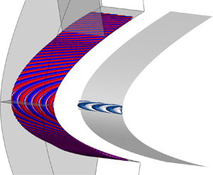
Figure 4(a,b) display the structures of direct and adjoint eigenvectors obtained from the largest R3 domain for the leading eigenvalues of CASES P2 and P8, respectively. The structures are visualized with the iso-surfaces of the real part of the direct spanwise velocity $\hat {w}$ and the adjoint spanwise velocity $\hat {w}^{{\dagger} }$. For both cases, red/blue colours stand for positive/negative values $(\pm 10^{-6}$) for direct eigenfunctions and blue/white colours represent positive/negative values ($\pm 10^{-3}$) for adjoint eigenfunctions. Figure 4(a,b) display the typical features for the direct global eigenfunctions exhibitting attachment-line instability near the leading edge, while either cross-flow instability (CASE P2) or second Mack mode (CASE P8) dominate downstream flows. For smaller $M_s$ (CASE P2), from the attachment-line plane, marked $a1$ in figure 4(a) and shown in figure 4(c), to the downstream plane, marked $a2$ in figure 4(a) and shown in figure 4(e), perturbations evolve away from wall surfaces forming cross-flow vortices aligned with external streamlines, as also reported by Mack et al. (Reference Mack, Schmid and Sesterhenn2008) and Meneghello et al. (Reference Meneghello, Schmid and Huerre2015). For larger $M_s$ (CASE P8), despite the similar mode structure at the attachment-line plane, marked $b1$ in figure 4(b) and shown in figure 4(d), the perturbations at the downstream plane, marked $b2$ in figure 4(b) and shown in figure 4(f), exhibit the behaviour of the second Mack mode instability with perturbations mainly located below the sonic line. In contrast to the feature that the perturbations of direct mode cover a large area, the adjoint mode appears only in the vicinity of the attachment line as shown in figure 4(a,b,g,h). Figure 4(g,h) show the contours of adjoint spanwise velocity $\hat {w}^{{\dagger} }$ for CASE P2 and P8 at the attachment-line planes, respectively. The basic structures of adjoint fields for both cases are similar and the bulk of adjoint fields moves away from the wall surface for large sweep Mach numbers. Moreover, based on the theoretical receptivity analysis on external force $\boldsymbol {f}$, this region is the most responsive to this discrete global mode. In other words, even though the direct global mode covers a large region further away from the attachment line, it is still possible to control/excite the mode by introducing forces at a relatively small region close to the attachment line. This finding is consistent with those from incompressible flows by Meneghello et al. (Reference Meneghello, Schmid and Huerre2015), indicating that the leading-edge control might be effective to the hypersonic flows over swept blunt bodies.

The characteristics of the leading attachment-line mode on sweep angles and the relative sweep Mach numbers are shown in figure 5. As the sweep angle varies from $20^{\circ }$ to $70^{\circ }$, the growth rate of the leading attachment-line mode shows a rising and then declining trend, reaching the locally highest point around $40^{\circ }$. When the sweep angle further increases, the growth rate of the leading attachment-line mode exhibits the features of monotonous increase and becomes positive again at large sweep Mach numbers. Moreover, this finding is consistent with two facts: the first is that the plane stagnation flow is known to be linearly stable for three-dimensional perturbations, as can be seen as the limit of zero sweep angle for the present cases; the other is that the attachment-line instability is found to become unstable for large sweep angles (Gaillard, Benard & Alziary de Roquefort Reference Gaillard, Benard and Alziary de Roquefort1999).

Figure 5. (a) Dependence of the growth rates on sweep Mach numbers. (b) Dependence of the frequency on sweep angle $\varLambda$. The marked red points represent CASES P1–P8.

Based on (2.23), the amplitudes of the modes excited by various boundary perturbations are mainly determined by the concomitant boundary term ($B.C.$). From the expression in Appendix A, it is clearly shown that the receptivity is evaluated from the gradients of adjoint variables and physical perturbations on the boundary. Moreover, this procedure permits the extraction of the receptivity amplitude pertaining to any discrete modes for any type of boundary perturbations at any location. Taking the surface perturbations in CASES P2 and P8, for instance, two types of surface perturbation (detailed expressions can be found in Appendix B) are calculated, as shown in figure 6. It demonstrates that the strong receptive regions of the leading attachment-line modes to surface perturbations are in the vicinity of attachment line and the surface perturbations at the exact attachment line are the most effective. Also, the surface vibrations are found to be a little more effective than suction/blowing, because of the higher excited amplitudes. Moreover, as the delta-function form perturbations are used and the basis for representation of LNSE cover the whole domain, the distributed surface perturbations receptivity analyses can be easily performed by integrations along the finite length. Further, as the present framework is from the basis of LNSE, the receptivity problem for the excitation of discrete modes of free-stream disturbances with surface inhomogeneities can be also taken into account.

Figure 6. Amplitudes of the leading attachment-line modes excited at different location $s/R$ for surface vibration and suction/blowing. All the eigenfunctions are normalized so that the density components on the wall surface are equal to one at the attachment line.

As mentioned by Tumin (Reference Tumin2020), the eigenfunction expansion methods for the two- and three-dimensional problems are the natural extensions of the widely used local cases. The analysis of discrete modes is similar for both local and global cases and can be easily performed. However, problems become more complicated with the continuous spectra since the mathematical properties of ordinary and partial differential operators are very different. Although uncertainties associated with the continuous spectra for global cases still exist, the bi-orthogonal eigenfunction system is still a powerful tool for solving global receptivity problems of discrete modes for complex high-speed boundary layers.