3.1. Dependence of thrust on Re, St and λ

Figure 4(a)–4(e) illustrates the dependence of ${\bar{C}_T}$ on Re, St and λ. The solid black line represents the drag–thrust boundary $({\bar{C}_T} = 0)$. For a given λ, the ${\bar{C}_T}$ increases from negative (lower-left corner) to positive (upper right corner) when St and Re are increased. The travelling wavy foil cannot produce thrust when Re and St are low but can when Re and St are sufficiently high, depending on λ. Interestingly, ${\bar{C}_T}$ is equally dependent on St and Re in the drag regime $({\bar{C}_T} < 0)$ but more sensitive to St in the thrust regime $({\bar{C}_T} > 0)$. This observation indicates that viscous (Re) and inertia (St) effects both play important roles in fluid dynamics in the drag regime while the inertia effect dictates the fluid dynamics in the thrust regime. For a given set of St and Re, an increase in λ leads to an enhancement in ${\bar{C}_T}$. As such, the drag–thrust boundary shifts to smaller St and Re when λ is increased. With the same St and λ, ${\bar{C}_T}$ gets higher at a higher Re, i.e. having acceleration is easier at a higher speed. The reason is that the viscous effect weakens and the added mass lessens (will be shown later) when Re is increased. On the other hand, a foil with a smaller λ hinders the streamwise flow over the surface, resulting in a smaller thrust generation. When the stationary wavy foil (St = 0) retains a travelling wavy shape (as sketched in figure 4a–e), it would experience a thrust $({\bar{C}_{T0}})$ that is negative (i.e. drag). Apparently, ${\bar{C}_{T0}}$ would be dependent on Re as shown in figure 4(f), where ${\bar{C}_{T0}}$ declines with Re as ${\bar{C}_{T0}} ={-} 6.13R{e^{ - 0.6}}$. Das, Shukla & Govardhan (Reference Das, Shukla and Govardhan2016) showed that a straight NACA0012 foil at zero attack angle incurs ${\bar{C}_{T0}} ={-} 5.96R{e^{ - 0.56}}$ that is smaller in magnitude than the present counterpart. This is plausible as an undulated foil would experience a higher drag than a straight foil.

Figure 4. (a–e) Dependence of time-mean thrust on Re, St and λ for the travelling wavy foil. A, B, C and D are four points selected as A (St = 0.2, Re = 100) in the drag regime, B (0.4, 250) close to drag–thrust boundary at high λ, C (0.6, 500) close to drag–thrust boundary at small λ and D (0.8,1000) in thrust regime, to show the influence of λ on instantaneous thrust in figure 9. (f) Dependence of time-mean thrust force of a stationary foil on Re. (a) $\lambda = 0.50$, (b) $\lambda = 0.67$, (c) $\lambda = 1.0$, (d) $\lambda = 1.5$, (e) $\lambda = 2.0$.

Based on the previous studies on the scaling of a flapping foil (Floryan et al. Reference Floryan, van Buren, Rowley and Smits2017; Van Buren et al. Reference Van Buren, Floryan, Quinn and Smits2017; Alam & Muhammad Reference Alam and Muhammad2020), the relationship of ${\bar{C}_T}$ with St, Re and λ can be written as

(3.1)\begin{equation}{\bar{C}_T} = {c_0}R{e^a}S{t^b}{\lambda ^c} + {\bar{C}_{T0}}.\end{equation}

Thus, λ naturally describes how the flow is transported from the leading edge to the trailing. When λ = 1, the flow transportation time T_λ (i.e. wave travelling time from the leading edge to the trailing) equals the travelling wavy motion period T. On the other hand, the T_λ > T and T_λ < T emerge at λ < 1 and λ > 1, respectively. This suggests that their relationship is linear, giving the exponent c of λ in (3.1) as c = 1. Based on the theoretical model involving the Euler angular, Coriolis and centrifugal accelerations of a cone of fluid around the foil, Alam & Muhammad (Reference Alam and Muhammad2020) theoretically showed that the relationship between ${\bar{C}_T}$ and St can be considered as ${\bar{C}_T} \propto S{t^3}$. Thus, (3.1) can be written as

(3.2)\begin{equation}{\bar{C}_T} = {c_0}R{e^a}S{t^3}{\lambda ^1} + {\bar{C}_{T0}}.\end{equation}

The linear least-squares regression for a given Re is used to find the relationship between ${\bar{C}_T}$, St and λ, giving ${\bar{C}_T} = {c_1}S{t^3}\lambda + {c_2}$, where four examples are illustrated in figure 5. The relationship provides c ₁ = 0.904, 1.388, 1.533 and 1.704 and c ₂ = −0.3848, −0.1543, −0.0951 and −0.061 for Re = 100, 500, 1000 and 2000, respectively (figure 5a–d). The dependence of c ₁ and c ₂ on Re (for all Re examined) can be observed from figure 6(a), where their dependencies are reprocessed as ${c_1} = 0.36R{e^{0.208}}$ and ${c_2} ={-} 6.13R{e^{ - 0.6}}$ (the ${\bar{C}_{T0}}$ scaling). Therefore, the relationship of ${\bar{C}_T}$ with St, Re and λ can be unified as

(3.3)\begin{equation}{\bar{C}_T} = 0.36R{e^{0.208}}S{t^3}\lambda - 6.13R{e^{ - 0.6}}.\end{equation}

Here, ${\bar{C}_{T0}} ={-} 6.13R{e^{ - 0.6}}$, with exponent −0.6 close to that of Re in $1/\sqrt {Re} $, indicates the dominance of fluid resistance forces from the unseparated boundary layer over the stationary foil surface. Equation (3.3) displays how St, Re and λ affect the propulsive force on the foil. It is easy to understand from (3.3) that the thrust generation $({\bar{C}_T} > 0)$ is largely dictated by St and $\lambda $, especially by St. The ${\bar{C}_T}$ grows slowly with increasing Re, which essentially reflects the viscous flow resistance weakening with increasing Re. In particular, when Re is large enough, the second term on the right-hand side approaches zero, which gives ${\bar{C}_T} = 0.36R{e^{0.208}}S{t^3}\lambda $. When the foil is stationary (St = 0), (3.3) degenerates into ${\bar{C}_T} ={-} 6.13R{e^{ - 0.6}}$, i.e. the ${\bar{C}_{T0}}$ scaling. To see how much (3.3) is capable of collapsing all simulated data, ${\bar{C}_T}$ is presented against $0.36R{e^{0.208}}S{t^3}\lambda - 6.13R{e^{ - 0.6}}$ in figure 6(b). The data for different values of λ collapse well on the line, suggesting that (3.3) can be used to estimate ${\bar{C}_T}$ for any values of St, Re and λ. Alam & Muhammad (Reference Alam and Muhammad2020) proposed a model of flow around a pitching hydrofoil. The flow model explicitly reflected the produced torque and thrust, involving Euler angular, Coriolis and centrifugal accelerations of a cone of fluid around the foil. They found that torque (power input) is required to compensate Euler and Coriolis accelerations, and thrust (output) is essentially produced from the centrifugal acceleration. The developed theoretical model showed that thrust is proportional to St ³.

Figure 5. Time-mean thrust coefficient ${\bar{C}_T}$ as a function of Strouhal number St and wavelength λ, denoted as ${\bar{C}_T} = {c_1}S{t^3}\lambda + {c_2}$. The dashed line is the linear least-squares regression line.

Figure 6. (a) Dependence of c ₁ and c ₂ on Re. (b) Relationship of ${\bar{C}_T}$ with St, Re and λ for the travelling wavy foil. The dashed lines denote the proportional function with coefficient equal to one.

Since Re appears in both terms on the right-hand side of (3.3), the dependence of ${\bar{C}_T}$ on Re may not be straightforward. We therefore calculate $\partial {\bar{C}_T}/\partial Re ( = 0.07488R{e^{ - 0.792}}S{t^3}\lambda + 3.678R{e^{ - 1.6}})$ from (3.3) to investigate the effect of Re on ${\bar{C}_T}$. Figure 7(a) displays $\partial {\bar{C}_T}/\partial Re$ against Re at St = 0.1, 0.5 and 1.0 with λ = 1.25. The value of $\partial {\bar{C}_T}/\partial Re$ declines with increasing Re regardless of St while a smaller St leads to a smaller $\partial {\bar{C}_T}/\partial Re$. The observation suggests that manoeuvring is easier at a smaller Re and a higher St. The value of $\partial {\bar{C}_T}/\partial Re$ sharply drops at $Re \le 250{-}600$ (depending on St) and reaches its asymptotically small value at $Re \ge 250{-}600$ (depending on St). That is, the effect of Re on ${\bar{C}_T}$ is predominant in the former Re range and insignificant in the latter Re range. To see how this information is dependent on λ and other St values, contours of $\partial {\bar{C}_T}/\partial Re$ are presented in the St--Re plane for different λ values examined (figure 7b). The value of $\partial {\bar{C}_T}/\partial Re$ degrades when λ is decreased, which can be observed from the higher $\partial {\bar{C}_T}/\partial Re$ region shrinking with decreasing λ. This again suggests that a higher λ is required for agility and manoeuvring. The $\partial {\bar{C}_T}/\partial Re$ contour can also be employed to understand the survival hydrodynamics of swimmers. A few interesting natural observations can be linked to the results in figure 7. Firstly, the prey is generally smaller in size than the concerned predator, hence the former having a smaller Re. This facilitates the prey having a greater agility or acceleration to escape from the predator. Secondly, a larger St and λ are beneficial to generating larger acceleration, which is consistent with Triantafyllou, Weymouth & Miao's (Reference Triantafyllou, Weymouth and Miao2015) observation that a swimmer usually adopts a larger St and λ during the predator–prey behaviour. When Re is sufficiently high due to increased speed, the Re effect disappears and the predator–prey game relies on St and λ only. Equation (3.3) further reflects that $\partial {\bar{C}_T}/\partial St$ is proportional to Re ^0.208 and λ, which suggests that the enhancement of ${\bar{C}_T}$ with St is larger at a higher Re and a larger λ. The scenario is also reflected in figure 4, with the contour lines having smaller slopes at smaller Re and vice versa. A predator usually large in size (hence higher Re) gets benefits of thrust enhancement with increasing St.

Figure 7. (a) Variation in $\partial {\bar{C}_T}/\partial Re$ with Re at λ = 1.25. (b) Relationship of $\partial {\bar{C}_T}/\partial Re$ with St, Re and λ.

The drag–thrust boundary $({\bar{C}_T} = 0)$ is found to be dependent on λ. It is worth finding the relationship between St, Re and λ corresponding to the drag–thrust boundary (figure 4). The drag–thrust boundary can be obtained from (3.3) by plugging ${\bar{C}_T} = 0$, i.e.

(3.4)\begin{equation}St = 2.57R{e^{ - 0.27}}{\lambda ^{ - 1/3}}.\end{equation}

Equation (3.4) reflects that the drag–thrust boundary in the St-Re domain advances with increasing λ, as illustrated in figure 4. This result conforms with the previous work by Gazzola et al. (Reference Gazzola, Argentina and Mahadevan2014). At a given λ, the boundary follows $St\mathrm{\ \propto }\, R{e^{ - 0.27}}$, which indicates that the drag–thrust boundary is more sensitive to St at smaller Re, and vice versa. The drag–thrust boundary can be considered as the native swimmer cruising at a constant speed, with no acceleration and no deceleration. Here, we again refer to the work of Gazzola et al. 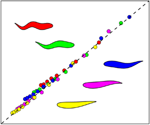(Reference Gazzola, Argentina and Mahadevan2014) where the locomotion of a cursing swimmer conforms to $St\mathrm{\ \propto\ }R{e^{ - 0.25}}$ when Re ≤ 2000. The present results and relationship conform with the biological observations (Gazzola et al. Reference Gazzola, Argentina and Mahadevan2014) while the effect of the deforming strategy (λ) on the cruising locomotion is first presented in this work (figure 8). When cruising in the water, different swimmers employ different deforming strategies, and hence different swimming strategies (e.g. St). It is the biological diversity of aquatic locomotion. Since λ values adopted by aquatic animals are restricted in a limited scope (Lucas et al. Reference Lucas, Johnson, Beaulieu, Cathcart, Tirrell, Colin, Gemmell, Dabiri and Costello2014), it is easy to understand that most cruising swimmers operate in a relatively narrow range of St, such as 0.2 ≤ St ≤ 0.4 (Taylor, Nudds & Thomas Reference Taylor, Nudds and Thomas2003; Eloy Reference Eloy2012; Gazzola et al. Reference Gazzola, Argentina and Mahadevan2014). In addition, the swimmer can generate accelerating or decelerating locomotion by increasing or decreasing λ, which provides a simple way to control the motion. For example, a swimmer can have a longer λ at the start of locomotion, a moderate λ to swim at a constant speed and a shorter λ to reduce the speed (deceleration).

Figure 8. Dependence of drag–thrust boundary on Strouhal number, Reynolds number and wavelength for the travelling wavy foil. The drag–thrust boundary corresponds to $St = 2.57R{e^{ - 0.27}}{\lambda ^{ - 1/3}}$ marked by the dashed line that fits well with the present data.

It should be noted that travelling wavy motion can be considered as the pitching motion when λ → ∞. We undertook numerical simulations for λ = 2.5, 3.0, 3.5, 4.0, 4.5, 5.0, 7.5, 10, 25, 50, 100, 1000, 10 000 and ∞ (straight foil, pitching) at St = 0.5 and Re = 1000 in order to understand how the results approach those for pitching motion of a straight foil. The foil kinematics gradually modifies from travelling wavy motion to pitching motion when λ is increased to ∞ (figure 9a). The foil with λ = ∞ corresponds to a pitching angle of 2.867°, given a ₁ = 0.05. Interestingly, ${\bar{C}_T}$ escalates for 0.50 ≤ λ ≤ 7.5 before declining for 7.5 < λ < 100. The value of ${\bar{C}_T}$ at λ = 100–10 000 is the same as that at λ = ∞ (figure 9b). The zoom-in view of figure 9(b) (shown as an inset) demonstrates that the linearity of ${\bar{C}_T}$ with λ (i.e. ${\bar{C}_T} \propto \lambda $) prevails at λ ≤ 2.5. To understand the thrust generation at λ > 100, simulations were conducted at λ = 1000 which provides the same ${\bar{C}_T}$ as λ = ∞ (figure 9b). Figure 9(c) shows ${\bar{C}_T}$ contours in the St–Re plane for St = 0.1–1.0 with ΔSt = 0.1 and Re = 50, 100, 250, 500, 750, 1000, 1250, 1500, 1750 and 2000. The value of ${\bar{C}_T}$ increases from negative to positive when St and Re are increased, where ${\bar{C}_T} < 0$ emerges at smaller Re and/or St, and ${\bar{C}_T} > 0$ is observed at larger Re and/or St, with the solid line $({\bar{C}_T} = 0)$ representing the drag–thrust boundary. Compared with the travelling wavy motion (figure 4), the pitching motion (λ = 1000 → ∞) produces a higher ${\bar{C}_T}$ with the drag–thrust boundary $({\bar{C}_T} = 0)$ shifting to a smaller Re and St.

Figure 9. (a) Change of foil shape with increasing λ; (b) dependence of ${\bar{C}_T}$ on λ at a ₁ = 0.05, St = 0.5 and Re = 1000; the blue-dashed line in the inset represents the linearity; (c) ${\bar{C}_T}$ contours in the St–Re plane at a ₁ = 0.05, λ = 1000, where the black solid line denotes the drag–thrust boundary.

Figure 10 displays C_T histories in one oscillation period at four selected points: A (St = 0.2, Re = 100) in drag regime, B (St = 0.4, Re = 250) close to the drag–thrust boundary at high λ, C (St = 0.6, Re = 600) close to the drag–thrust boundary at small λ and D (St = 0.8, Re = 1000) in thrust regime, all marked in the St-Re map (figure 4). Similar to the previous works on the pitching foil (Koochesfahani Reference Koochesfahani1989), two C_T peaks are observed in the upstroke and downstroke. The travelling wavy foil experiences drag during the entire period at St = 0.2, Re = 100 (figure 10a). For the given St and Re, the C_T peak becomes larger when λ increases from 0.50 to 2.0. At intermediate St and Re values (points B and C), the foil undergoes both drag and thrust in the period (figure 10b,c). On the other hand, at a higher St and Re, only thrust acts on the foil in the entire period (figure 10d). The C_T amplitude (the gap between maximum and minimum) grows with increasing St, Re and λ (figure 10a–d). A smaller λ, therefore, engenders a more steady thrust, which explains the swimming behaviour of the anguilliform swimmer. On the other hand, the maximum instantaneous thrust generated for a higher λ explicates why the slender swimmer usually employs the C-start strategy during the survival behaviour (Gazzola et al. Reference Gazzola, van Rees and Koumoutsakos2012). More discussion on the instantaneous thrust coefficient is provided in Appendix A.3.

Figure 10. The instantaneous thrust coefficient for the travelling wavy foil in one oscillation period. In (a), ${\bar{C}_T} ={-} 0.423$, −0.416, −0.407, −0.392 and −0.386 for λ = 0.50, 0.67, 1.0, 1.5 and 2.0, respectively; in (b), ${\bar{C}_T} ={-} 0.212$, −0.185, −0.176, −0.101 and −0.052 for λ = 0.50, 0.67, 1.0, 1.5 and 2.0, respectively; in (c), ${\bar{C}_T} ={-} 0.026$, 0.056, 0.207, 0.468 and 0.637 for λ = 0.50, 0.67, 1.0, 1.5 and 2.0, respectively; and in (d), ${\bar{C}_T} = 0.230$, 0.402, 0.746, 1.311 and 1.687 for λ = 0.50, 0.67, 1.0, 1.5 and 2.0, respectively. (a) $St = 0.2,Re = 100$, (b) $St = 0.4,Re = 250$, (c) $St = 0.6,Re = 500$ and (d) $St = 0.8,Re = 1000$.

The total thrust acting on the travelling wavy foil consists of a friction drag (negative thrust) and a form thrust (positive or negative), i.e. C_T = C_Tp + C_Tf, where C_Tp and C_Tf denote the instantaneous pressure and friction thrust coefficients, respectively. Naturally, ${\bar{C}_T} = {\bar{C}_{Tp}} + {\bar{C}_{Tf}}$. Figure 11 shows the dependence of ${\bar{C}_{Tp}}$, ${\bar{C}_{Tf}}$ and ${\bar{C}_T}$ on St and Re. At a moderate Re of 1000, the dependence of ${\bar{C}_{Tp}}$, ${\bar{C}_{Tf}}$ and ${\bar{C}_T}$ on St = 0.1–1.0 and λ = 0.5–2.0 is illustrated in figure 11(a). With increasing St, ${\bar{C}_{Tp}}$ grows from negative to positive while ${\bar{C}_{Tf}}$ remains negative and linearly decreases, regardless of λ (figure 11a). To understand the dependence of ${\bar{C}_{Tp}}$ and ${\bar{C}_{Tf}}$ on St, we made polynomial fit to the curves as ${\bar{C}_{Tp}} = {c_{0p}} + {c_{1p}}St + {c_{2p}}S{t^2} + {c_{3p}}S{t^3}$ and ${\bar{C}_{Tf}} = {c_{0f}} + {c_{1f}}St$. The curve fitting provided ${c_{2p}} \approx 0.001 \approx 0$ regardless of λ while c _1p and c _1f were almost equal in magnitude but opposite in sign. The total thrust can, therefore, be written as ${\bar{C}_T} = {\bar{C}_{Tp}} + {\bar{C}_{Tf}} = ({c_{0p}} + {c_{0f}}) + {c_{3p}}S{t^3}$. For a stationary foil (St = 0), ${c_{0p}} + {c_{0f}} = {\bar{C}_{T0}}$, which makes ${\bar{C}_T} = {\bar{C}_{T0}} + {c_{3p}}S{t^3}$. The polynomial fit of ${\bar{C}_{Tp}}$ and linear fit of ${\bar{C}_{Tf}}$ are presented in figure 11(a), where the data derived from different St values collapse well on the lines. When λ increases, ${\bar{C}_{Tp}}$ rapidly grows while ${\bar{C}_{Tf}}$ does not significantly change. That is, the effect of λ on ${\bar{C}_T}$ is largely determined by ${\bar{C}_{Tp}}$. Figure 11(b) displays the Re effect on ${\bar{C}_{Tp}}$, ${\bar{C}_{Tf}}$ and ${\bar{C}_T}$ at St = 0.5 at different λ values. With increasing Re, the magnitude of ${\bar{C}_{Tf}}$ (negative in the entire range of Re) diminishes rapidly at Re ≤ 500 but mildly at Re > 500. In other words, ${\bar{C}_{Tf}}$ is more sensitive to Re for Re ≤ 500 than for Re > 500. On the other hand, the reduction of ${\bar{C}_{Tp}}$ at Re ≤ 500 is not as much as that of the ${\bar{C}_{Tf}}$ magnitude, ${\bar{C}_{Tp}}$ remaining more or less constant at Re > 500. As such, ${\bar{C}_T}$ grows more rapidly at Re ≤ 500 than at Re > 500. Again, with increasing λ, the ${\bar{C}_{Tf}}$ distribution does not change appreciably while ${\bar{C}_{Tp}}$ enhances significantly, as does ${\bar{C}_T}$. The observation conforms with the dependence of ${\bar{C}_T}$ on Re and λ presented in figure 7.

Figure 11. Effects of (a) St and (b) Re on ${\bar{C}_{Tp}}$, ${\bar{C}_{Tf}}$ and ${\bar{C}_T}$; (a) Re = 1000 and (b) St = 0.5.

Figure 12(a) shows the distributions of the local time-mean pressure thrust coefficient $\bar{C}_{Tp}^s$ along the foil, where s varying from 0 to L is the distance measured from the leading edge. As expected, $\bar{C}_{Tp}^s/\textrm{|}{\bar{C}_{Tp}}\textrm{|}$ is negative near the leading edge for λ ≤ 2.0 (figure 12a1–a5). As marked by the red-dashed circles for λ = 0.50 (figure 12a1), there are two $\bar{C}_{Tp}^s/\textrm{|}{\bar{C}_{Tp}}\textrm{|}$ peaks at s/L = 0.26 and 0.76, the latter being 4.6 times higher than the former. The trailing edge (s/L = 0.90–1.00) largely undergoes negative thrust while the positive thrust is largely generated at 0.55 < s/L < 0.90. With increasing λ from 0.5 to 2.0 (figure 12a1–a5), (i) $\bar{C}_{Tp}^s/\textrm{|}{\bar{C}_{Tp}}\textrm{|}$ near the leading edge does not change appreciably, remaining negative for s/L < 0.07–0.14 depending on λ, (ii) the first peak weakens, losing its identity for λ ≥ 1.0, (iii) the second peak shifts toward the middle, becoming wider and blunt and (iv) the negative thrust near the trailing edge reduces in magnitude, becoming positive at λ = 2.0. Figure 12(a6) shows the $\bar{C}_{Tp}^s/\textrm{|}{\bar{C}_{Tp}}\textrm{|}$ distribution at λ = ∞ to understand the trend for the widely studied pitching foil. The trend $\bar{C}_{Tp}^s/\textrm{|}{\bar{C}_{Tp}}\textrm{|} > \textrm{0}$ emerges at all s/L values. When λ increases from 2.0 to ∞, the peak $\bar{C}_{Tp}^s/\textrm{|}{\bar{C}_{Tp}}\textrm{|}$ is further postponed from s/L = 0.55 to 0.69, with the peak magnitude declining from 1.90 to 1.42.

Figure 12. (a) Distributions of local time-mean pressure thrust coefficient $\bar{C}_{Tp}^s/|{\bar{C}_{Tp}}|$ along the foil. (b) Contributions from the anterior, mid and posterior bodies on pressure thrust. Here, (St, Re) = (0.5, 1000).

From the $\bar{C}_{Tp}^s/\textrm{|}{\bar{C}_{Tp}}\textrm{|}$ distributions (figure 12a), it is worth seeing the contributions of anterior, mid and posterior bodies to pressure thrust. Following Lucas, Lauder & Tytell (Reference Lucas, Lauder and Tytell2020), we define the anterior, mid and posterior bodies as 0.00 ≤ s/L ≤ 0.10, 0.10 < s/L ≤ 0.55 and 0.55 < s/L ≤ 1.00, respectively. The contributions δ_p of the three portions to pressure thrust are estimated as

(3.5)\begin{equation}{\delta _p} = \left\{ {\begin{array}{*{20}{l}} {\dfrac{{\int_{0.00}^{0.10} {\bar{C}_{Tp}^s\,\textrm{d(}s\textrm{/}L)} }}{{{{\bar{C}}_{Tp}}}}}&{\textrm{for}\;\textrm{anterior}\;\textrm{body}}\\ {\dfrac{{\int_{0.10}^{0.55} {\bar{C}_{Tp}^s\,\textrm{d(}s\textrm{/}L)} }}{{{{\bar{C}}_{Tp}}}}}&{\textrm{for}\;\textrm{mid}\;\textrm{body}}\\ {\dfrac{{\int_{0.55}^{1.00} {\bar{C}_{Tp}^s\,\textrm{d(}s\textrm{/}L)} }}{{{{\bar{C}}_{Tp}}}}}&{\textrm{for}\;\textrm{posterior}\;\textrm{body}} \end{array}} \right..\end{equation}

The corresponding results are presented in figure 12(b). The anterior body provides a negative contribution (δ_p < 0), small in magnitude, to the pressure thrust for all λ values. With increasing λ, δ_p for the mid body firstly increases for 0.50 ≤ λ ≤ 1.0 and then declines for 1.0 ≤ λ ≤ 2.0, while the posterior body shows an opposite scenario. In other words, the posterior body provides the largest δ_p = 83.18 % at the smallest λ = 0.50 examined, and the mid body renders the greatest δ_p = 72.76 % at λ = 1.0. Their contributions are comparable at the largest λ = 2.0 examined. At λ = ∞ (figure 12b6), δ_p for the mid body shrinks while that for the posterior body grows to 55 %, a 12 % increase from λ = 2.0. This result conforms to the previous works on the pitching foil (e.g. Das et al. Reference Das, Shukla and Govardhan2016; Alam & Muhammad Reference Alam and Muhammad2020) as well as the biological observations (Lucas et al. Reference Lucas, Lauder and Tytell2020). In particular, Alam & Muhammad (Reference Alam and Muhammad2020) showed that the pressure field over the pitching foil characterizes the inertial effects and determines the thrust generation. The observations suggest that for the anguilliform swimmers with a smaller λ (e.g. the eel, Lindsey Reference Lindsey1978), the pressure thrust is mainly generated from the posterior oscillation, while both mid and posterior are equally important to generate pressure thrust for the carangiform (e.g. mackerel, Lindsey Reference Lindsey1978) and thunniform swimmers (e.g. tuna, Lindsey Reference Lindsey1978) with λ > 1.0.

Figure 13(a) shows local time-mean friction thrust $\bar{C}_{Tf}^s$ distributions along the foil. The entire foil undergoes negative $\bar{C}_{Tf}^s$. In the anterior region, the $\bar{C}_{Tf}^s/\textrm{|}{\bar{C}_{Tf}}\textrm{|}$ plummets immediately behind the leading edge and then grows rapidly. The increase in $\bar{C}_{Tf}^s/\textrm{|}{\bar{C}_{Tf}}\textrm{|}$ is rather mild in the mid region while the second half of the posterior region has a decreasing $\bar{C}_{Tf}^s/\textrm{|}{\bar{C}_{Tf}}\textrm{|}$. Interestingly, the minimum $\bar{C}_{Tf}^s/\textrm{|}{\bar{C}_{Tf}}\textrm{|}$ in the anterior region rises with increasing λ while that in the posterior region drops. The influence of λ on $\bar{C}_{Tf}^s/\textrm{|}{\bar{C}_{Tf}}\textrm{|}$ is less in the mid region than in the other two regions. With λ increasing from 2.0 to ∞, $\bar{C}_{Tf}^s/\textrm{|}{\bar{C}_{Tf}}\textrm{|}$ magnitudes at the leading and trailing edges become smaller and larger, respectively. A native swimmer uses lateral lines as sensors to achieve the flow information (e.g. pressure and shear stress around itself) and hence to make a swimming decision, while the lateral lines are mainly distributed at the head and caudal fin of a fish (Sapède et al. Reference Sapède, Gompel, Dambly-Chaudière and Ghysen2002). Recently, Verma et al. (Reference Verma, Papadimitriou, Lüthen, Arampatzis and Koumoutsakos2020) studied optimal sensor configurations that enable swimmers to maximize the information gathered from their surrounding flow field. At λ ≈ 1.0, it is noted that the shear stress sensors should be densely distributed in the anterior and in the second half of the posterior regions of the swimmer.

Figure 13. (a) Distributions of local time-mean friction thrust coefficient $\bar{C}_{Tf}^s/|{\bar{C}_{Tf}}|$ along the foil. (b) Contributions from the anterior, mid and posterior bodies on friction thrust. Here, (St, Re) = (0.5, 1000).

Similar to the definition of δ_p in (3.6), we employed δ_f to denote the contributions of anterior, mid and posterior bodies to the friction thrust. When λ grows from 0.50 to 2.0, figure 13(b) depicts that the δ_f decreases from 28.05 % to 21.71 % for the anterior body and from 43.44 % to 32.92 % for the mid body, while increasing from 28.51 % to 45.37 % for the posterior body. For λ ≤ 2.0, δ_f > 20 % for the anterior, mid and posterior regions, which suggests that the contributions from all portions are significant. The increase in λ from 2 to ∞ leads to declining δ_f for the anterior and mid bodies but increasing δ_f for the posterior body. At λ = ∞, the posterior body undergoes δ_f = 50.24, an 11 % increase from λ = 2, which suggests that the posterior body is the main contributor to the friction drag.

3.2. Dependence of added mass, added damping and efficiency on Re, St and λ

For the undulating swimmer, the added mass plays a dominant role in the propulsive performance (Lighthill Reference Lighthill1970, Candelier, Boyer & Leroyer Reference Candelier, Boyer and Leroyer2011, Eloy, Reference Eloy2012, Paniccia et al. Reference Paniccia, Graziani, Lugni and Piva2021). In the elongated-body theory (Lighthill Reference Lighthill1970), the added mass per unit length at the foil trailing edge can be calculated from a curvilinear coordinate system as ρ ${\rm \pi}$h ²/4, where h denotes the thickness of the foil and is assumed to be smaller enough, i.e. $h \ll L$. As Lighthill's theory is inviscid, the viscous influence is neglected, while recent work reveals that the resistive mechanism is also crucial for the inertial undulatory swimmers (Piñeirua, Godoy-Diana & Thiria Reference Piñeirua, Godoy-Diana and Thiria2015). Both h/L and Re effects cannot be ignored in the case of viscous flow. It is thus worth understanding how the added mass is affected by St, Re and λ and how it impacts the thrust and power.

Generally, the total fluid added mass m_a due to the foil oscillation can be calculated as

(3.6)\begin{equation}{m_a} = \int_0^{{L_s}} {{m_x}\,\textrm{d}x} ,\end{equation}

where x is measured from the leading edge and m_x denotes the added mass for an elemental length dx (figure 14a). A summation can be considered to replace the integral in (3.6), i.e.

(3.7)\begin{equation}{m_a} = \sum\limits_{n = 1}^{n = N} {{m_n}} ,\end{equation}

where n is the number of sample slices of the foil. The difference in the estimated m_a between N = 20 and 30 is found to be less than 1 %. The value N = 20 is adopted (figure 14a). Each slice is assumed to be sinusoidally oscillating in the vertical direction. Thus, m_n can be calculated using the equation introduced by Qin, Alam & Zhou (Reference Qin, Alam and Zhou2017) for an oscillating cylinder, as

(3.8)\begin{equation}{m_n} = \frac{{{F_{Ln}}\cos \phi }}{{{\omega ^2}{Y_n}}},\end{equation}

where F_Ln is the amplitude of the time-dependent lift force ${F_L}(t) = {F_{Ln}}\sin (\omega t + \phi )$ at slice n, Y_n is the amplitude of the displacement of slice n with $Y(t) = {Y_n}\sin (\omega t)$, ϕ is the phase shift between F_L(t) and Y(t) and ω = 2${\rm \pi}$/T. Note that the m_n is the effective added mass, not the potential added mass (Williamson & Govardhan Reference Williamson and Govardhan2004). The added mass ratio $m_a^\ast $ can then be estimated as

(3.9)\begin{equation}m_a^\ast = \frac{{{m_a}}}{{{m_f}}},\end{equation}

where m_f is the mass of fluid displaced by the foil. In our paper, the effective added mass is calculated from the component of the fluid force in phase with the foil acceleration ((3.7)–(3.9)). The effective added mass includes both potential added mass and flow-induced added mass (Konstantinidis, Dorogi & Baranyi Reference Konstantinidis, Dorogi and Baranyi2021; Alam Reference Alam2022). As a result, the effective added mass can be positive or negative, as shown in figure 14(b1). More discussion on the relationship between the effective added mass and potential added mass can be found in Facchinetti, de Langre & Biolley (Reference Facchinetti, de Langre and Biolley2004) and Han & de Langre (Reference Han and de Langre2022).

Figure 14. (a) Sketches for the sampling slices. Effects of St, Re and λ on (b) $m_a^\ast $, (c) c_a, (d) ${\bar{C}_{pi}}$ and (e) η. Here, (b1, c1, d1, e1) Re = 1000, and (b2, c2, d2, e2) St = 0.5.

How $m_a^\ast $ is contingent on St and Re is illustrated in figure 14(b). When Re = 1000 (figure 14b1), $m_a^\ast $ is negative at St = 0.1, and its magnitude gets large with increasing λ. On the other hand, $m_a^\ast $ is positive at St ≥ 0.2, increasing with increasing St and λ. Note that a negative $m_a^\ast $ makes the foil lighter to move, while a positive $m_a^\ast $ makes the foil heavier. The value of $m_a^\ast $ is a stronger function of St at a larger λ. The effect of Re on $m_a^\ast $ can be understood from figure 14(b2), where $m_a^\ast $ declines with increasing in Re, particularly at Re ≤ 500, regardless of λ. The viscous effect on $m_a^\ast $ becomes negligible when Re is sufficiently large. On the other hand, λ has a strong influence on $m_a^\ast $, the higher the λ, the larger the $m_a^\ast $.

The effect of St, Re and λ on the out-of-phase component of the lift force (i.e. added damping) is also considered. Recalling the work of Qin et al. (Reference Qin, Alam and Zhou2017), the added damping of the travelling wavy foil can be defined as

(3.10)\begin{equation}{c_a} = \sum\limits_{n = 1}^{n = N} {{c_n}} ,\end{equation}

where

(3.11)\begin{equation}{c_n} ={-} \frac{{{F_{Ln}}\sin \phi }}{{\omega {Y_n}}}.\end{equation}

As shown in figure 14(c), St and Re have effects on c_a, where c_a reduces with increasing St and/or Re, and c_a < 0 at St = 0.5 for all tested Re values. The case c_a > 0 is only observed at λ = 0.50, 0.67 and 1.0 with St = 0.1 (figure 14c1). The declination of c_a with increasing St is larger at a larger λ (figure 14c1). As such, the larger the St, the greater the c_a decrease with increasing λ. Since a negative c_a implies the flow assisting the motion, the contribution by the flow is constructive to ${\bar{C}_T}$ when St, Re and λ all are increased (figure 4).

The effect of St and Re on the input power ${\bar{C}_{pi}}$ required to move the foil is depicted in figure 14(d). The total power is composed of power P_s associated with oscillation and power P_T associated with thrust (Shen et al. Reference Shen, Zhang, Yue and Triantafyllou2003; Dong & Lu Reference Dong and Lu2005). The former is required to produce the lateral oscillations of the foil while the latter is needed to generate the thrust force. The mathematical definitions of P_s and P_T are as follows:

(3.12)\begin{equation}{P_s} ={-} \oint {(f_y^p + f_y^f)} {[1 + {(1 + \textrm{d}y\textrm{/d}t)^2}]^{1/2}}\frac{{\textrm{d}y}}{{\textrm{d}t}}\,\textrm{d}x,\end{equation}

and

(3.13)\begin{equation}{P_T} ={-} {F_x}(t)U,\end{equation}

where $\mathrm{\oint }$ denotes the integration along the foil surface, $f_y^p ={-} p$ and $f_y^f = \; \mu [2(\partial v/\partial y) - (\textrm{d}y/\textrm{d}x)(\partial v/\partial x + \partial u/\partial y)]$ with u and v representing the velocity components in the x and y directions, respectively. Thus, time-mean power coefficient ${\bar{C}_{pi}}$ in one oscillation period is defined as

(3.14)\begin{equation}{\bar{C}_{pi}} = \frac{1}{T}\int_t^{t + T} {\frac{{{P_s} + {P_T}}}{{0.5\rho {U^3}L}}\,\textrm{d}t} .\end{equation}

As illustrated in figure 14(d1), ${\bar{C}_{pi}}$ exponentially grows with increasing St, approximately following ${\bar{C}_{pi}} \propto S{t^3}$. Alam & Muhammad (Reference Alam and Muhammad2020) mathematically showed that the input power of a pitching foil is highly sensitive to St and varies as the cube of St. For a given St, a larger ${\bar{C}_{pi}}$ is required for a larger λ for St ≥ 0.2 while ${\bar{C}_{pi}}$ deceases with increasing λ at St = 0.1 (inset of figure 14d1), which coincides with the relationship of $m_a^\ast $ with λ (figure 14b). The ${\bar{C}_T}$ scaling in (3.4) echoes that ${\bar{C}_T}$ values at St = 0.1 for different λ values are close to each other, with only a 2.36 % difference in ${\bar{C}_T}$ between λ = 0.50 and 2.0. As such, P_s is the dominant factor contributing to ${\bar{C}_{pi}}$. A shorter λ, therefore, causes a higher ${\bar{C}_{pi}}$ at St = 0.1 (see the inset of figure 14d1). When St ≥ 0.2, P_T gradually dominates P_s where a longer λ complements a larger ${\bar{C}_T}$ (figure 4). It should be noted that St ≥ 0.5 (depending on λ) provides positive ${\bar{C}_T}$ (figure 11a), hence aquatic animals may use St ≥ 0.5. The relationship of ${\bar{C}_{pi}}$ with Re (figure 14d2) is similar to that of $m_a^\ast $ with Re (figure 14b2). Overall, a large λ corresponds to a larger $m_a^\ast $ and a higher ${\bar{C}_{pi}}$ for St ≥ 0.2. The dependence of $m_a^\ast $ on λ evokes that a slender tail or a slender swimming body cannot have a large λ because a large $m_a^\ast $ makes the tail or body heavier, so it is difficult for the animal to oscillate its tail/body, given that it has limited strength and limited rigidity of the tail. It could thus be said that a longer tail/body may adopt a shorter λ. For example, the λ employed by eel swimmers is shorter than that used by trout (Webb Reference Webb1984). Biological observations of Gray (Reference Gray1933) provided similar conclusions.

It is also worth investigating how the propulsive efficiency is affected by St, Re and λ. Here, the foil's propulsive efficiency is calculated via

(3.15)\begin{equation}\eta = {\bar{C}_T}/{\bar{C}_{pi}}.\end{equation}

Using ${\bar{C}_T}$ data in figure 11 and ${\bar{C}_{pi}}$ data in figure 14(d), we obtained the relationship of η with St, Re and λ in figure 14(e). Following the sign of ${\bar{C}_T}$ in figure 11(a), η < 0 at a smaller St (figure 14e1). When St passes the drag–thrust boundary (3.4), i.e. $St > 2.57R{e^{ - 0.27}}{\lambda ^{ - 1/3}}$, the foil can generate positive thrust $({\bar{C}_T} > 0)$ (figure 11a) and thus a positive efficiency (figure 14e1). The value of η increases for a certain range of St, reaching a maximum before declining, except for λ = 0.50 where η keeps increasing with St up to St = 1.0. While the maximum efficiency value is weakly dependent on λ, the St value corresponding to the maximum efficiency is smaller at a larger λ, i.e. η = 14.67 % for (St, λ) = (1.0, 0.50), η = 15.63 % for (St, λ) = (0.9, 0.67), η = 15.87 % for (St, λ) = (0.8, 1.0), η = 15.03 % for (St, λ) = (0.5, 1.5) and η = 14.26 % for (St, λ) = (0.5, 2.0), see inset of figure 14(e1). The data indicate that λ = 1.0 renders the largest η. That is, the aquatic swimmers can achieve a higher propulsive efficiency by employing λ ≈ 1.0, which is in agreement with the biological observations from swimming fish (Videler Reference Videler1993). Figure 14(e2) shows the effect of Re on η, where η increases with Re. At 50 < Re ≤ 500, a larger λ leads to a higher η, while λ = 1.5 and 1.0 cause the higher η at 750 < Re ≤ 1500 and 1750 < Re ≤ 2000, respectively.

Besides the effects of St, Re and λ on $m_a^\ast $, it is also worth understanding the distribution of m_n along the foil length, i.e. n = 1 - 20. Here, m_n is normalized as $m_n^\ast = {m_n}/{m_f}$. As shown in figure 15, $m_n^\ast $ is highly dependent on n for large λ (≥ 1.0) values, where it is large (positive) near the midspan (n = 7 - 15) and negative near the leading edge of the foil. At small λ = 0.50 and 0.67 each, $m_n^\ast $ displays small peaks at n = 4 and 17.

Figure 15. The $m_n^\ast $ at different slices; St = 0.5 and Re = 1000.

3.3. Flow structures

Following the above discussion on thrust generation, the associated flow structures are presented to gain the physical insight into fluid dynamics around the swimmer. Seven distinguished wake structures are identified in the St–Re domain examined: steady wake (+ symbol), quasi Kármán vortex (q-KV) wake ( symbol), quasi reverse Kármán vortex (q-RKV) wake ( symbol), KV wake (○ symbol), 2S (two single) aligned wake (■ symbol), RKV wake (δ symbol) and slanted reverse Kármán vortex (s-RKV) wake (∇ symbol). The representative flow structures and their presence in the St–Re domain are shown in figures 16 and 17. The steady wake is observed at $St \le 0.6$ and $Re \le 250$ (figures 16a and 17), where the wake is steady, similar to the flow structure behind a quiescent foil (St = 0). With a little increase in St and/or Re, the steady wake transmutes to q-KV wake (figure 16b) or q-RKV wake (figure 16c) representing a transition from a steady wake to a classical KV or RKV wake. The q-KV and q-RKV wakes form at low and high St, respectively, the former prevailing for smaller λ (≤1.0) only (figure 17). Here, Kármán or reverse Kármán vortices form immediately behind the foil, vanishing rapidly to generate a steady wake downstream (figure 16a–c). The generation of a steady wake followed by a Kármán wake was also found in the wake of a fixed elliptical cylinder at Re = 100–150 in Shi, Alam & Bai (Reference Shi, Alam and Bai2020a) and Shi et al. (Reference Shi, Alam, Bai and Wang2020b). Depending on λ, when Re is further increased, a KV wake forms, featuring negative and positive vortices above and below the foil symmetry line correspondingly (figure 16d). The 2S aligned wake refers to the case where both positive and negative vortices lie on the symmetric line (figure 16e). The 2S aligned wake is considered as the boundary between KV and RKV wakes, and has been extensively discussed in previous works (Godoy-Diana et al. Reference Godoy-Diana, Aider and Wesfreid2008, Reference Godoy-Diana, Marais, Aider and Wesfreid2009; Marais et al. Reference Marais, Thiria, Wesfreid and Godoy-Diana2012; Deng et al. Reference Deng, Sun and Shao2015, Reference Deng, Sun, Teng, Pan and Shao2016; Andersen et al. Reference Andersen, Bohr, Schnipper and Walther2017; Chao et al. Reference Chao, Pan, Zhang and Yan2019; Chao et al. Reference Chao, Alam, Ji and Wang2021b). The emergence of the 2S aligned wake at the KV–RKV boundary (red dashed line) precedes the drag–thrust boundary (black solid line) in the St--Re map (figure 17). The same is true for a pitching foil (Godoy-Diana et al. Reference Godoy-Diana, Aider and Wesfreid2008). With a further increase in St and/or Re, the RKV wake emerges, where the negative and positive vortices nestle oppositely to those of KV wake (figure 16f). In the s-RKV wake, the symmetric line of two vortex streets does not coincide with the foil symmetric line. The slant direction can be upward or downward. The downward slanted RKV is referred to as the ds-RKV wake (figure 16g) while the upward slanted RKV is referred to as the us-RKV wake (figure 16h). The slant direction of the s-RKV wake is also affected by λ, see figure 16(g,h). Generally, the slant direction strongly depends on the first vortex pair generated by the foil (Zheng & Wei Reference Zheng and Wei2012). Here, both the ds-RKV and us-RKV wakes are considered as an s-RKV wake because the physical mechanisms of the ds-RKV and us-RKV wakes are identical. The formation of the slanted wake is also common in flow-induced vibrations of cylinders (Bhatt & Alam Reference Bhatt and Alam2018).

Figure 16. Typical instantaneous vorticity structures: (a) steady wake (St, Re, λ = 0.2, 100, 1.0); (b) q-KV wake (St, Re, λ = 0.4, 100, 1.0); (c) q-RKV wake (St, Re, λ = 0.7, 100, 1.0); (d) KV wake (St, Re, λ = 0.3, 1000, 1.0); (e) 2S aligned wake (St, Re, λ = 0.3, 2000, 1.0); (f) RKV wake (St, Re, λ = 0.5, 1000, 1.0); (g) downward slanted reverse Kármán vortex (ds-RKV) wake (St, Re, λ = 0.8, 1000, 1.0); and (h) upward slanted reverse Kármán vortex (us-RKV) wake (St, Re, λ = 0.8, 1000, 1.5).

Figure 17. The wake structure map with the black solid line denoting the drag–thrust boundary, red dashed line denoting the KV–RKV wake boundary and blue dash-dotted line denoting the RKV-s-RKV wake boundary. Here, A, B, C and D are four points selected as A (St = 0.2, Re = 100) in drag regime, B (0.4, 250) close to the drag–thrust boundary at high λ, C (0.6, 600) close to drag-thrust boundary at small λ and D (0.8,1000) in thrust regime to show the influence of λ on flow structures in figure 17. Here, (a) $\lambda = 0.50$, (b) $\lambda = 0.67$, (c) $\lambda = 1.0$, (d) $\lambda = 1.5$ and (e) $\lambda = 2.0$.

Figure 17 also shows how λ affects the wakes behind a travelling wavy foil, particularly the transition between two different types of flow structures. For example, the KV–RKV wake transition bordered by the 2S aligned wake advances with increasing λ. Similarly, the RKV–s-RKV wake transition (blue dash-dotted line) also shifts to smaller St and/or Re when λ is increased. In addition, there is no s-RKV wake observed at λ = 0.50 (figure 17a). Physically, λ describes how the foil locomotion propagates from the leading to trailing edges. Therefore, the foil's horizontal acceleration at the trailing edge declines with the decrease in λ. As a result, the convection velocity of the vortices with respect to U also decreases with declining λ. In the previous work, Godoy-Diana et al. (Reference Godoy-Diana, Marais, Aider and Wesfreid2009) showed that the generation of the s-RKV wake is significantly dependent on the value of this convection velocity, where a larger value of this convection velocity may induce an s-RKV wake. A smaller λ thus postpones the transition between RKV and s-RKV wakes.

To evaluate quantitatively the influence of St, Re and λ on vortex strength in different regimes, figure 18 presents dimensionless spanwise vorticity ω* (= ωL/U) structures at the four selected points located in the St--Re plane (figure 17). The value of ω* increases with St, Re and λ, which is consistent with the change in ${\bar{C}_T}$ in figure 4. A similar relationship of the spatial wavelength Δd with St, Re and λ is noticeable, having the same correspondence with ${\bar{C}_T}$. The growth of Δd with St and Re is ascribed to the increased velocity of vortices when St and Re are increased. On the other hand, it is easy to understand that a smaller λ would lead to a smaller velocity of the vortices, hence a smaller Δd and ${\bar{C}_T}$.

Figure 18. Contours of spanwise vorticity ${\omega ^\ast } = \omega L/U$. The red and blue colours denote positive and negative ${\omega ^\ast }$, respectively.

Figure 19(a) illustrates the effect of St on the wake structure at Re = 1000 and λ = 1.0. A couple of observations can be made here. First, when St is increased, the wake structure transmutes from the KV wake (figure 19a1) into the RKV wake (figures 19a2 and 19a3) and then into the s-RKV wake (figures 19a4–19a6). Second, the streamwise spatial wavelength of vortices in the vortex street shrinks with increasing St, i.e. vortices are densely distributed for a higher St. Third, an increase in St enhances vorticity magnitudes of vortices in the wake. Based on the definition of the St (2.2), one can understand that the increase in St corresponding to a decrease in the undulating period T causes an increase in acceleration and velocity of the foil tail, and hence results in the enhancement of vorticity (Das et al. Reference Das, Shukla and Govardhan2016; Alam & Muhammad Reference Alam and Muhammad2020; Muhammad, Alam & Noack Reference Muhammad, Alam and Noack2022). Figure 19(b) shows how Re affects the wake structures at St = 0.8 and λ = 1.0. When Re is increased, the wake structure modifies from RKV to s-RKV, and vorticity magnitudes rise. Since Re physically describes the fluid resistance, it is easy to understand that ω* and ${\bar{C}_T}$ increase when Re increases (figure 4c). Also, the slant angle of the RKV wake gradually rises when Re increases from 1000 to 2000, which ties in with the work on a pitching foil by Das et al. (Reference Das, Shukla and Govardhan2016).

Figure 19. Effects of (a) St and (b) Re on flow patterns; (a) Re = 1000 and (b) St = 0.8.

3.4. Effect of λ on velocity and pressure on the foil

Figure 20 illustrates the instantaneous relative streamwise velocity $u_r^\ast ( = u/U - 1)$ snapshots at y/L = 0.15 (upper side) and −0.15 (lower side), where u denotes the instantaneous streamwise velocity. Three λ values, i.e. λ = 0.50, 1.0 and 2.0, are presented. Here $u_r^\ast $ can be considered as the indicator of local momentum transport in the streamwise direction. It is thus connected to the generation of thrust. It is worth understanding which part of the foil is crucial for generating thrust, particularly when λ is short.

Figure 20. Variation of $u_r^\ast = (u/U - 1)$ over the foil at y/L = 0.15 (red dashed line) and y/L = −0.15 (green dash-dotted line), where u is the local instantaneous streamwise velocity. The black solid line denotes the foil centreline profile; (St, Re) = (0.5, 1000) with (a) $\lambda = 0.50$, (b) $\lambda = 1.0$ and (c) $\lambda = 2.0$.

The $u_r^\ast $ profiles following the foil shape form waves and propagate from the leading edge to the trailing edge. At y/L = 0.15 (red dashed line), the peaks in $u_r^\ast $ occur close to the troughs of the foil wave for a short λ and before the troughs for a long λ. An opposite scenario is observed for the $u_r^\ast $ profile at y/L = −0.15. That is, the travelling of the V-shaped buckets on the upper side and overturned V-shaped buckets on the lower side is mainly responsible for the momentum transport in the streamwise direction in the case of a short λ. On the other hand, for a long λ, both lateral oscillation of foil and streamwise travel of the buckets contribute to the streamwise momentum transport, given that $u_r^\ast $ peaks precede the troughs.

Consider a slice of the foil (yellow backdrop, figure 20a3) forming an overturned V-shaped bucket where a fluid mass over the upper surface of the foil tends to move downstream but is hindered by the crest of the foil. As a result, $u_r^\ast $ on the upper side is negative, with minimum $u_r^\ast $ corresponding to the crest of the foil. On the other hand, the fluid mass beneath the lower surface of the foil is pushed downstream by the travelling wave, which results in the increased $u_r^\ast $. For a longer λ (figure 20b4), each point of the foil's geometry experiences both lateral and horizontal motion. The crests or valleys of the foil shape do not coincide with those of $u_r^\ast $.

Figure 21 shows the evolution of the pressure coefficient ${C_p} = (p - \; {p_\infty })/0.5\rho {U^2}$ pattern with changing λ at St = 0.5 and Re = 1000, where p _∞ is the free-stream pressure. The pressure pattern appears complex at λ = 0.50 (figure 20a). With t/T = 0.25, the pressure around the crests and troughs (upper side) is negative and positive, respectively, as the crests have downward accelerations and the troughs have upward accelerations (see pointing arrows). The low and high pressure on the crests and troughs increase and their regions shift downstream from t/T = 0.25 to 0.50 following the movement of the foil wave. The pressure is generally larger in the V-shaped or overturned V-shaped buckets than that on other sides (see figures for t/T = 0.25–1.0). This explains that the bucket movement in the streamwise direction engenders streamwise momentum transport. Similar observations are made for λ = 1.0 (figure 21b). At λ = 2.0 (figure 21c), when the trailing edge of the foil moves downwards (green arrow) at t/T = 0.25, the lower and upper trailing surfaces of the foil undergo high and low pressure, respectively. Since the foil tail is bent upward with its maximum amplitude, the positive and negative pressures appear on the lower and upper trailing surfaces, respectively. At t/T = 0.50 where the foil is concave up near the middle (red arrow) with the leading and trailing edges aligned with y/L = 0, the pressure is positive on the concave side and negative on the convex side. Naturally, the pressure patterns at t/T = 0.75 and 1.0 are opposite to those at t/T = 0.25 and 0.50, respectively.

Figure 21. Evolution of pressure coefficient C_p in one undulating period at St = 0.5 and Re = 1000. The arrows denote the moving direction. (a) $\lambda = 0.50$, (b) $\lambda = 1.0$ and (c) $\lambda = 2.0$.