


1 Introduction
The discretization of differential equations is a necessity of life—most differential equations cannot be solved analytically, and a discrete numeric solution is the choice approach for many applications. However, by their nature, discrete differences lose “associativity” preserved in continuous derivatives [Reference Gadish, Griniasty and Lawrence6]. A recent programme attempts to cure this problem by constructing a discrete analogue to differential geometry with C-infinity structure [Reference Lawrence, Ranade and Sullivan8]. The starting point is to associate a differential graded Lie algebra (DGLA) with cell complexes.
For a regular CW complex
 $X$
, it is possible to associate a DGLA model
$X$
, it is possible to associate a DGLA model
 $A=A(X)$
over
$A=A(X)$
over
 $\mathbb {Q}$
satisfying the following conditions:
$\mathbb {Q}$
satisfying the following conditions:
-
• as a completed graded Lie algebra,
 $A(X)$
is freely generated by a set of generators, one for each cell in
$X$
and whose grading is one less than the geometric degree of the cell;
$A(X)$
is freely generated by a set of generators, one for each cell in
$X$
and whose grading is one less than the geometric degree of the cell; -
• vertices (that is,
$0$
-cells) in
$X$
give rise to generators a that satisfy the Maurer–Cartan equation
$\partial a+\frac 12[a,a]=0$
(a flatness condition); -
• for a cell
$x$
in
$X$
, the part of
${\partial }{x}$
without Lie brackets is the geometric boundary
${\partial }_0x$
(where an orientation must be fixed on each cell); -
• (locality) for a cell
$x$
in
$X$
,
${\partial }{x}$
lies in the completed Lie algebra generated by the generators of
$A(X)$
associated with cells of the closure
$\bar {x}$
.


The existence and general construction of such a model was demonstrated by Sullivan in the Appendix to [Reference Tradler and Zeinalian11]; however, the procedure given there is an iterative algorithm. By [Reference Buijs, Félix, Murillo and Tanré1], there exist consistent (even symmetric) towers of models of simplices, and such towers are unique up to (exact) DGLA isomorphism. The explicit (unique) model associated with the interval was found in [Reference Lawrence and Sullivan10]. Explicit symmetric models of two-dimensional cells were demonstrated in previous work for bi-gons (see [Reference Gadish5,Reference Gadish, Griniasty and Lawrence6]) and arbitrary n-gons (see [Reference Griniasty and Lawrence7]), the main intermediate step being the construction of a ‘symmetric point’ in the model of the boundary of the cell, invariant under the full symmetries of the cell. In this paper we explicitly construct for the first time DGLA models of
 $3$
-cells, in particular for a banana-shaped cell (see Theorem 3.3) and for a cube (see Section 4), that are invariant under symmetries fixing a major diagonal.
$3$
-cells, in particular for a banana-shaped cell (see Theorem 3.3) and for a cube (see Section 4), that are invariant under symmetries fixing a major diagonal.
In Section 2, we give a collection of general facts about DGLAs and models of cell complexes (some reproduced from [Reference Griniasty and Lawrence7, Reference Lawrence and Sullivan10]), including defining the notion of a point (solution of MC), of a particular
 $k$
-cell
$k$
-cell
 $(k>1)$
being localised at a point in a model, how to ‘twist’ a model so as to move the points of localisation of cells as well as the universal averages of [Reference Lawrence and Siboni9]. In Section 3, we construct a symmetric model of the
$(k>1)$
being localised at a point in a model, how to ‘twist’ a model so as to move the points of localisation of cells as well as the universal averages of [Reference Lawrence and Siboni9]. In Section 3, we construct a symmetric model of the
 $n$
-faceted banana in which the main cell is localised at a symmetric central point, by first constructing a model localised at one of the vertices of the banana and then twisting it. In Section 4, we derive a model of an arbitrary polyhedral
$n$
-faceted banana in which the main cell is localised at a symmetric central point, by first constructing a model localised at one of the vertices of the banana and then twisting it. In Section 4, we derive a model of an arbitrary polyhedral
 $3$
-cell and give the example of the cube where the induced model is invariant under those symmetries of the cube fixing a main diagonal; this model will be used in [Reference Lawrence, Ranade and Sullivan8].
$3$
-cell and give the example of the cube where the induced model is invariant under those symmetries of the cube fixing a main diagonal; this model will be used in [Reference Lawrence, Ranade and Sullivan8].
2 General Properties of DGLAs and DGLA Models
2.1 General DGLAs
For simplicity, we will work over
 $k=\mathbb {Q}$
, though the discussion also holds for any field of characteristic zero. Recall that a DGLA over k is a vector space A over
$k=\mathbb {Q}$
, though the discussion also holds for any field of characteristic zero. Recall that a DGLA over k is a vector space A over
 $k$
with
$k$
with
 $\mathbb {Z}$
-grading
$\mathbb {Z}$
-grading
 $A=\oplus _{n\in \mathbb {Z}}A_n$
along with a bilinear map
$A=\oplus _{n\in \mathbb {Z}}A_n$
along with a bilinear map
 $[\cdot ,\cdot ]{\colon }{}A\times {}A\rightarrow {}A$
(bracket, respecting the grading) and a linear map
$[\cdot ,\cdot ]{\colon }{}A\times {}A\rightarrow {}A$
(bracket, respecting the grading) and a linear map
 ${\partial }{\colon }{}A\rightarrow {}A$
(differential, grading shift
${\partial }{\colon }{}A\rightarrow {}A$
(differential, grading shift
 $-1$
) for which
$-1$
) for which
 ${\partial }^2=0,$
while
${\partial }^2=0,$
while
-
symmetry of bracket
$[b,a]=-(-1)^{|a||b|}[a,b];$
-
Jacobi identity
$(-1)^{|a||b|}[[b,c],a]+(-1)^{|b||c|}[[c,a],b]+(-1)^{|c||a|}[[a,b],c]=0;$
-
Leibniz rule
${\partial }[a,b]=[{\partial }{a},b]+(-1)^{|a|}[a,{\partial }{b}],$


for all homogeneous
 $a,b,c\in {}A$
. Defining the adjoint action of A on itself by
$a,b,c\in {}A$
. Defining the adjoint action of A on itself by
 ${\mathrm {ad}}_e(a)=[e,a]$
, the operator
${\mathrm {ad}}_e(a)=[e,a]$
, the operator
 ${\text {ad}}_e{\colon } A\rightarrow {}A$
has grading shift
${\text {ad}}_e{\colon } A\rightarrow {}A$
has grading shift
 $|e|$
, for homogeneous
$|e|$
, for homogeneous
 $e\in {}A$
. The Jacobi identity and Leibniz rule can now be reformulated as operator equalities:
$e\in {}A$
. The Jacobi identity and Leibniz rule can now be reformulated as operator equalities:
-
Jacobi identity
${\text {ad}}_{[a,b]}=[{\text {ad}}_a,{\text {ad}}_b]$
; -
Leibniz rule
${\text {ad}}_{{\partial }{a}}=[{\partial },{\text {ad}}_a]$
;


in terms of the graded operator commutator,
 $[A,B]\equiv {}A\circ {}B-(-1)^{|A||B|}B\circ {}A$
. Since the relations all preserve the number of brackets, it is meaningful to define an additional grading by the number of (Lie) brackets; in particular, for
$[A,B]\equiv {}A\circ {}B-(-1)^{|A||B|}B\circ {}A$
. Since the relations all preserve the number of brackets, it is meaningful to define an additional grading by the number of (Lie) brackets; in particular, for
 $x\in {}A$
, let
$x\in {}A$
, let
 $x^{[m]}$
denote the part of x containing precisely
$x^{[m]}$
denote the part of x containing precisely
 $m$
brackets.
$m$
brackets.
2.2 Points and Localisation
An element
 $a\in {}A_{-1}$
is called a point (or is said to be flat) in the model if it satisfies the Maurer–Cartan equation
$a\in {}A_{-1}$
is called a point (or is said to be flat) in the model if it satisfies the Maurer–Cartan equation
 ${\partial }{a}+{\tfrac 12}[a,a]=0$
. For any point
${\partial }{a}+{\tfrac 12}[a,a]=0$
. For any point
 $a\in {}A_{-1}$
, define the twisted differential
$a\in {}A_{-1}$
, define the twisted differential
 ${\partial }_a$
by
${\partial }_a$
by
 ${\partial }_a\equiv {\partial }+{\text {ad}}_a$
; the fact that
${\partial }_a\equiv {\partial }+{\text {ad}}_a$
; the fact that
 ${\partial }_a^2=0$
is guaranteed by the Maurer–Cartan condition. By the localisation of A to a point
${\partial }_a^2=0$
is guaranteed by the Maurer–Cartan condition. By the localisation of A to a point
 $a$
, denoted
$a$
, denoted
 $A(a)$
, we will mean the DGLA that as a graded Lie algebra is
$A(a)$
, we will mean the DGLA that as a graded Lie algebra is
 $$\begin{align*}(\ker{\partial}_a|_{A_0})\oplus\bigoplus_{n>0}A_n\end{align*}$$
with the induced bracket from A and the differential
 ${\partial }_a$
. This contains only non-negative gradings. Leibniz guarantees that
${\partial }_a$
. This contains only non-negative gradings. Leibniz guarantees that
 $\ker {\partial }_a|_{A_0}$
is closed under Lie bracket.
$\ker {\partial }_a|_{A_0}$
is closed under Lie bracket.
2.3 Edges and Flows
Any element
 $e\in {}A_0$
defines a flow on A by
$e\in {}A_0$
defines a flow on A by
 $$ \begin{align} \frac{dx}{dt}={\partial}{e}-{\text{ad}}_e(x)\quad\text{on}\quad A_{-1}\>,\qquad \frac{dx}{dt}=-{\text{ad}}_e(x)\quad\text{on}\quad A_{\not=-1}. \end{align} $$
This flow is called the flow by
 $e$
and preserves the grading. (To define this rigorously, one can work in a space quotiented by all expressions involving
$e$
and preserves the grading. (To define this rigorously, one can work in a space quotiented by all expressions involving
 $N+1$
Lie brackets, as in [Reference Lawrence and Sullivan10], effectively truncating to the space of linear combinations of terms involving at most
$N+1$
Lie brackets, as in [Reference Lawrence and Sullivan10], effectively truncating to the space of linear combinations of terms involving at most
 $N$
Lie brackets, whose coefficients are polynomials in
$N$
Lie brackets, whose coefficients are polynomials in
 $t$
with rational coefficients. Then one considers the tower of spaces as
$t$
with rational coefficients. Then one considers the tower of spaces as
 $N$
increases. Equivalently, one can choose a basis for the finite-dimensional space of expressions involving exactly
$N$
increases. Equivalently, one can choose a basis for the finite-dimensional space of expressions involving exactly
 $N$
Lie brackets, and then allowed expressions are formal combinations of these basis elements, over all
$N$
Lie brackets, and then allowed expressions are formal combinations of these basis elements, over all
 $N$
, with coefficients that are polynomials in
$N$
, with coefficients that are polynomials in
 $t$
. While we talk about functions of
$t$
. While we talk about functions of
 $t$
and their derivatives, these are well defined for rational
$t$
and their derivatives, these are well defined for rational
 $t$
, with derivatives being well-defined, since all the coefficients are polynomial functions of
$t$
, with derivatives being well-defined, since all the coefficients are polynomial functions of
 $t$
.)
$t$
.)
Lemma 2.1 For any
 $e\in {}A_0$
, the flow by
$e\in {}A_0$
, the flow by
 $e$
in grading
$e$
in grading
 $-1$
preserves flatness. That is, if
$-1$
preserves flatness. That is, if
 $x(t)\in {}A_{-1}$
satisfies (2.1) with initial condition
$x(t)\in {}A_{-1}$
satisfies (2.1) with initial condition
 $x(0)$
satisfying the Maurer–Cartan condition, then at any (rational) time
$x(0)$
satisfying the Maurer–Cartan condition, then at any (rational) time
 $t$
,
$t$
,
 $x(t)$
also satisfies Maurer–Cartan.
$x(t)$
also satisfies Maurer–Cartan.
Proof As in the proof of [Reference Lawrence and Sullivan10, Theorem 1], consider the curvature
 $f(t)\in {}A_{-2}$
defined by
$f(t)\in {}A_{-2}$
defined by
 $f\equiv {}{\partial }{x}+{\frac 12}[x,x]$
. It satisfies
$f\equiv {}{\partial }{x}+{\frac 12}[x,x]$
. It satisfies
 $$ \begin{align*} \frac{df}{dt}&={\partial}\frac{dx}{dt}+\Big[x,\frac{dx}{dt}\Big]=-{\partial}({\text{ad}}_ex)+[x,{\partial}{e}]-[x,{\text{ad}}_e(x)]\\ &=-{\partial}\circ{\text{ad}}_e(x)+{\text{ad}}_{{\partial}{e}}(x)+({\text{ad}}_x)^2e=-{\text{ad}}_e\circ{\partial}(x)+{\tfrac12}{\text{ad}}_{[x,x]}e=-{\text{ad}}_ef\>, \end{align*} $$
a first order homogeneous linear ode for
 $f(t)$
with initial condition
$f(t)$
with initial condition
 $f(0)=0$
, since
$f(0)=0$
, since
 $x(0)$
satisfies the Maurer–Cartan condition. Thus,
$x(0)$
satisfies the Maurer–Cartan condition. Thus,
 $f(t)=0$
for all
$f(t)=0$
for all
 $t$
, as required. ▪
$t$
, as required. ▪
Linearity of the differential equations (2.1) in e ensures that flowing by
 $e$
for time t is equivalent to flowing by
$e$
for time t is equivalent to flowing by
 $te$
for a unit time. Denote the result of flowing by
$te$
for a unit time. Denote the result of flowing by
 $e$
from
$e$
from
 $a\in {}A_{-1}$
for unit time, by
$a\in {}A_{-1}$
for unit time, by
 $u_e(a)$
, so that the solution of the first equation in (2.1) is
$u_e(a)$
, so that the solution of the first equation in (2.1) is
 $x(t)=u_{te}(x(0))$
. Explicitly,
$x(t)=u_{te}(x(0))$
. Explicitly,
 $$\begin{align*}u_e(a)=e^{-{\text{ad}}_e}a+\frac{1-e^{-{\text{ad}}_e}}{{\text{ad}}_e}{\partial}{e} =a+{\partial}{e}-[e,a+\tfrac12{\partial}{e}]+(\geq2\ \text{brackets}),\end{align*}$$
where the meaning of the operator quotient is the series
 $\sum _{n=0}^\infty \frac {(-1)^n}{(n+1)!}({\text {ad}}_e)^n({\partial }{e})$
.
$\sum _{n=0}^\infty \frac {(-1)^n}{(n+1)!}({\text {ad}}_e)^n({\partial }{e})$
.
Lemma 2.2 For a point
 $a$
, the condition that
$a$
, the condition that
 $u_e(a)=a$
is equivalent to
$u_e(a)=a$
is equivalent to
 ${\partial }_ae=0$
, that is,
${\partial }_ae=0$
, that is,
 $e\in {}A(a)_{0}$
(
$e\in {}A(a)_{0}$
(
 $e$
is localised at
$e$
is localised at
 $a$
). This is a linear condition on
$a$
). This is a linear condition on
 $e,$
and therefore, in this case, the flow by
$e,$
and therefore, in this case, the flow by
 $e$
fixes
$e$
fixes
 $a$
at all time (not only after unit time).
$a$
at all time (not only after unit time).
Lemma 2.3 (see [Reference Gadish, Griniasty and Lawrence6, Lemma 2.2])
If
 $e$
flows from a point
$e$
flows from a point
 $a$
to a point
$a$
to a point
 $b$
in unit time, then
$b$
in unit time, then
 ${\partial }_b\circ \exp (-{\text {ad}}_e)=\exp (-{\text {ad}}_e)\circ {\partial }_a$
so that
${\partial }_b\circ \exp (-{\text {ad}}_e)=\exp (-{\text {ad}}_e)\circ {\partial }_a$
so that
 $\exp (-{\text {ad}}_e)$
intertwines the localisation
$\exp (-{\text {ad}}_e)$
intertwines the localisation
 $A(a)$
to the localisation
$A(a)$
to the localisation
 $A(b)$
.
$A(b)$
.
Example 2.4 The unique DGLA model,
 $A(I)$
, of an interval has three generators;
$A(I)$
, of an interval has three generators;
 $a,\;b$
of grading
$a,\;b$
of grading
 $-1$
(the endpoints), and
$-1$
(the endpoints), and
 $e$
of grading
$e$
of grading
 $0$
(the 1-cell). The differential is given by the condition
$0$
(the 1-cell). The differential is given by the condition
 $u_e(a)=b$
(see [Reference Lawrence and Sullivan10]). Explicitly,
$u_e(a)=b$
(see [Reference Lawrence and Sullivan10]). Explicitly,
 $$\begin{align*}{\partial}{e}=({\text{ad}}_e)b+\sum\limits_{i=0}^\infty{\frac{B_i}{i!}}({\text{ad}}_e)^i(b-a)=\frac{E}{1-e^E}a+\frac{E}{1-e^{-E}}b=b-a+\tfrac{E}2(a+b)+\cdots,\end{align*}$$
where
 $B_i$
denotes the
$B_i$
denotes the
 $i$
-th Bernoulli number defined as coefficients in the expansion
$i$
-th Bernoulli number defined as coefficients in the expansion
 $\frac {x}{e^x-1}=\sum _{n=0}^\infty {}B_n \frac {x^n}{n!}$
,
$\frac {x}{e^x-1}=\sum _{n=0}^\infty {}B_n \frac {x^n}{n!}$
,
 $E\equiv {\text {ad}}_e,$
and the expressions in
$E\equiv {\text {ad}}_e,$
and the expressions in
 $E$
are considered as formal power series.
$E$
are considered as formal power series.
Example 2.5 In any DGLA model
 $A(X)$
of a regular cell complex
$A(X)$
of a regular cell complex
 $X$
, for any
$X$
, for any
 $1$
-cell
$1$
-cell
 $e$
in
$e$
in
 $X$
with endpoints
$X$
with endpoints
 $a,\;b$
, there is a natural DGLA homomorphism
$a,\;b$
, there is a natural DGLA homomorphism
 $A(I)\rightarrow {}A(X)$
, while
$A(I)\rightarrow {}A(X)$
, while
 $u_e(a)=b$
.
$u_e(a)=b$
.
Denote by
 ${\text {BCH}}(x,y)$
the Baker–Campbell–Hausdorff formula for the element of the free Lie algebra (over
${\text {BCH}}(x,y)$
the Baker–Campbell–Hausdorff formula for the element of the free Lie algebra (over
 $\mathbb {Q}$
) in two variables
$\mathbb {Q}$
) in two variables
 $x,\;y$
such that as formal series
$x,\;y$
such that as formal series
 $\exp (x).\exp (y)=\exp {\text {BCH}}(x,y)$
(see [Reference Eichler4] for a short proof of existence and [Reference Dynkin3] for a computational formula). Here, we collect some elementary properties that follow from the definition, Jacobi, and uniqueness of
$\exp (x).\exp (y)=\exp {\text {BCH}}(x,y)$
(see [Reference Eichler4] for a short proof of existence and [Reference Dynkin3] for a computational formula). Here, we collect some elementary properties that follow from the definition, Jacobi, and uniqueness of
 $\mathrm{BCH}$
as a free Lie algebra element.
$\mathrm{BCH}$
as a free Lie algebra element.
-
(i) The first few terms of
${\text {BCH}}(x,y)$
are where
$$ \begin{align*} {\text{BCH}}(x,y)=x+y&+\frac{1}{2}[x,y]+\frac{1}{12}(X^2y+Y^2x)-\frac{1}{24}XYXy\!+\!\cdots, \end{align*} $$
$X,Y$
denote
${\text {ad}}_x,{\text {ad}}_y$
.
-
(ii)
${\text {BCH}}({\text {ad}}_x,{\text {ad}}_y)={\text {ad}}_{{\text {BCH}}(x,y)}$
. -
(iii)
$\mathrm{BCH}$
is associative; that is,
${\text {BCH}} ({\text {BCH}}(x,y),z )={\text {BCH}} (x,{\text {BCH}}(y,z) )$
for any symbols
$x,y,z$
. The iterated
$\mathrm{BCH}$
of n symbols
$x_1,\dots {}x_n\in {}A$
will be written
${\text {BCH}}(x_1,\dots ,x_n)$
.


Lemma 2.7 There is a homomorphism from the group
 $A_0$
considered with operation
$A_0$
considered with operation
 ${\text {BCH}}$
, to the group
${\text {BCH}}$
, to the group
 ${\text {Aut}}(A)$
, defined by mapping
${\text {Aut}}(A)$
, defined by mapping
 $e\in {}A_0$
to the flow (in unit time) as defined on all gradings in A by equation (2.1).
$e\in {}A_0$
to the flow (in unit time) as defined on all gradings in A by equation (2.1).
Proof By [Reference Lawrence and Sullivan10, Lemma 3], and the explicit formula given for
 $u_e(a)$
above, it follows that
$u_e(a)$
above, it follows that
 $$\begin{align*}u_{e_2}\big(u_{e_1}(a)\big)=u_{{\text{BCH}}(e_1,e_2)}(a)\>,\end{align*}$$
for any
 $a\in {}A_{-1}$
. Thus, on elements of grading
$a\in {}A_{-1}$
. Thus, on elements of grading
 $-1$
, a flow by
$-1$
, a flow by
 $e_1$
for unit time followed by a flow by
$e_1$
for unit time followed by a flow by
 $e_2$
for unit time is equivalent to a flow by
$e_2$
for unit time is equivalent to a flow by
 ${\text {BCH}}(e_1,e_2)$
for unit time. Note that the flow for unit time by e acting on
${\text {BCH}}(e_1,e_2)$
for unit time. Note that the flow for unit time by e acting on
 $A_n$
for
$A_n$
for
 $n\not =-1$
, is just the exponential operator
$n\not =-1$
, is just the exponential operator
 $\exp (-{\text {ad}}_e)$
for which it is immediate that
$\exp (-{\text {ad}}_e)$
for which it is immediate that
 $\exp (-{\text {ad}}_{e_2})\circ \exp (-{\text {ad}}_{e_1})=\exp (-{\text {ad}}_{\mathrm{BCH}(e_1,e_2)})$
.▪
$\exp (-{\text {ad}}_{e_2})\circ \exp (-{\text {ad}}_{e_1})=\exp (-{\text {ad}}_{\mathrm{BCH}(e_1,e_2)})$
.▪
Definition 2.8 By a piecewise linear path
 $\gamma $
in
$\gamma $
in
 $A$
, we mean a sequence of points
$A$
, we mean a sequence of points
 $a_i\in {}A_{-1}$
(
$a_i\in {}A_{-1}$
(
 $0\leq {}i\leq {}m$
) along with elements
$0\leq {}i\leq {}m$
) along with elements
 $e_i\in {}A_0$
(
$e_i\in {}A_0$
(
 $1\leq {}i\leq {}m$
), called edges, which are such that the edges define flows between the respective points, that is,
$1\leq {}i\leq {}m$
), called edges, which are such that the edges define flows between the respective points, that is,
 $u_{e_i}(a_{i-1})=a_i$
for all
$u_{e_i}(a_{i-1})=a_i$
for all
 $1\leq {}i\leq {}m$
. For such a path, we denote by
$1\leq {}i\leq {}m$
. For such a path, we denote by
 ${\text {BCH}}(\gamma )\in {}A_0$
the iterated
${\text {BCH}}(\gamma )\in {}A_0$
the iterated
 $\mathrm{BCH}$
of the edges,
$\mathrm{BCH}$
of the edges,
 ${\text {BCH}}(\gamma )\equiv {\text {BCH}}(e_1,\dots ,e_m)$
. A piecewise linear path in
${\text {BCH}}(\gamma )\equiv {\text {BCH}}(e_1,\dots ,e_m)$
. A piecewise linear path in
 $A$
is called a loop if its initial and final points agree, that is
$A$
is called a loop if its initial and final points agree, that is
 $a_0=a_m$
.
$a_0=a_m$
.
Lemma 2.9 (see [Reference Buijs, Félix, Murillo and Tanré2])
If
 $X$
has
$X$
has
 $c$
connected components and
$c$
connected components and
 $\{a_1,\dots ,a_c\}$
is a choice of basepoints, one in each connected component, then the set of points in
$\{a_1,\dots ,a_c\}$
is a choice of basepoints, one in each connected component, then the set of points in
 $A(X)$
is
$A(X)$
is
 $$\begin{align*}\bigcup\limits_{i=1}^c\big\{u_e(a_i)\bigm|e\in{}A_0\big\}\cup \big\{u_e(0)\bigm|e\in{}A_0\big\}\>.\end{align*}$$
For each
 $i$
, the map
$i$
, the map
 $\pi _i{\colon }{}e\mapsto {}u_e(a_i)$
is a ‘fibration’, with fibre
$\pi _i{\colon }{}e\mapsto {}u_e(a_i)$
is a ‘fibration’, with fibre
 $\pi _i^{-1}(a_i)$
generated as a vector space by
$\pi _i^{-1}(a_i)$
generated as a vector space by
 $\{{\text {BCH}}(\gamma )|\gamma \in \pi _1(X,a_i)\}$
, while the map
$\{{\text {BCH}}(\gamma )|\gamma \in \pi _1(X,a_i)\}$
, while the map
 $\pi _0{\colon }{}e\mapsto {}u_e(0)$
is injective.
$\pi _0{\colon }{}e\mapsto {}u_e(0)$
is injective.
2.4 Localisation of Models
As noted in Section 1,
 $A(X)$
is not unique, but is well defined up to (exact) DGLA isomorphism.
$A(X)$
is not unique, but is well defined up to (exact) DGLA isomorphism.
Definition 2.10 A point
 $a\in {}A_{-1}$
in a model of a regular cell complex
$a\in {}A_{-1}$
in a model of a regular cell complex
 $X$
is said to be local to a cell
$X$
is said to be local to a cell
 $f$
in
$f$
in
 $X$
if it lies in the submodel generated by the cells in the closure
$X$
if it lies in the submodel generated by the cells in the closure
 $\overline {f}$
of
$\overline {f}$
of
 $f$
.
$f$
.
By Lemma 2.9, equivalently, a point is local to the cell
 $f$
if it can be written as
$f$
if it can be written as
 $u_e(a_0)$
, where
$u_e(a_0)$
, where
 $a_0$
is a 0-cell in
$a_0$
is a 0-cell in
 $\overline {f}$
and
$\overline {f}$
and
 $e$
is a zero-graded element in the (free) Lie algebra generated by cells in
$e$
is a zero-graded element in the (free) Lie algebra generated by cells in
 $\overline {f}$
.
$\overline {f}$
.
Definition 2.11 In a DGLA model
 $A$
of a regular cell complex
$A$
of a regular cell complex
 $X$
, a
$X$
, a
 $k$
-cell
$k$
-cell
 $f$
(for
$f$
(for
 $k>1$
) will be said to be localised at the point
$k>1$
) will be said to be localised at the point
 $a\in {}A_{-1}$
if
$a\in {}A_{-1}$
if
 ${\partial }_af={\partial }{}f+[a,f]$
lies in the (free) Lie algebra generated by cells of the closure of the geometric boundary
${\partial }_af={\partial }{}f+[a,f]$
lies in the (free) Lie algebra generated by cells of the closure of the geometric boundary
 $\overline {{\partial }_0f}$
.
$\overline {{\partial }_0f}$
.
Here, by abuse of notation, we have used the same symbol for the geometric
 $k$
-cell
$k$
-cell
 $f$
and the element
$f$
and the element
 $f\in {}A_{k-1}$
in its model. By locality of the model and using freeness of the Lie algebra, we see that the point of localisation of a cell
$f\in {}A_{k-1}$
in its model. By locality of the model and using freeness of the Lie algebra, we see that the point of localisation of a cell
 $f$
in a model (if it exists) is unique and must be local to the cell (in the sense of Definition 2.10).
$f$
in a model (if it exists) is unique and must be local to the cell (in the sense of Definition 2.10).
Remark The explicit constructions of models of the bi-gon in [Reference Gadish, Griniasty and Lawrence6] and the triangle in [Reference Griniasty and Lawrence7], are localised (at their ‘centre’ points). Although not all models of
 $X$
will be such that all cells of dimension
$X$
will be such that all cells of dimension
 $>1$
are localised (for example in the model of the bi-gon in [Reference Gadish5], the main cell is not localised at any point), we will see in Section 4 that such models always exist in dimensions up to three. A similar construction should also work in higher dimensions.
$>1$
are localised (for example in the model of the bi-gon in [Reference Gadish5], the main cell is not localised at any point), we will see in Section 4 that such models always exist in dimensions up to three. A similar construction should also work in higher dimensions.
Lemma 2.12 If A is a model of a regular cell complex
 $X$
in which the
$X$
in which the
 $k$
-cell
$k$
-cell
 $f$
(
$f$
(
 $k>1$
) is localised at the point
$k>1$
) is localised at the point
 $a\in {}A_{-1}$
, then for any
$a\in {}A_{-1}$
, then for any
 $e\in {}A_0$
in the subalgebra generated by the 1-skeleton of
$e\in {}A_0$
in the subalgebra generated by the 1-skeleton of
 $\overline {f}$
, there is a variation
$\overline {f}$
, there is a variation
 $A'$
of the model in which the generator for f is replaced by
$A'$
of the model in which the generator for f is replaced by
 $$\begin{align*}f'=\exp(-{\text{ad}}_e)\cdot{}f\end{align*}$$
and the cell
 $f$
is localised at the point
$f$
is localised at the point
 $a'=u_e(a)$
.
$a'=u_e(a)$
.
Proof This is immediate from Lemma 2.3,
 ${\partial }_{a'}f'=\exp (-{\text {ad}}_e)\cdot {\partial }_af$
. ▪
${\partial }_{a'}f'=\exp (-{\text {ad}}_e)\cdot {\partial }_af$
. ▪
The above lemma means that we can ‘twist’ any model in which a cell is localised, so that the cell is localised at any point we please (which is local to the cell). This technique was used in [Reference Gadish, Griniasty and Lawrence6, Reference Griniasty and Lawrence7] to generate symmetric models, by writing first a (non-symmetric) model of the relevant
 $2$
-cell localised at a point on its boundary and then twisting it so that it is localised at a symmetric point. All that remained was to verify that the model obtained was indeed symmetric.
$2$
-cell localised at a point on its boundary and then twisting it so that it is localised at a symmetric point. All that remained was to verify that the model obtained was indeed symmetric.
Remark Since the 1-skeleton of
 $\overline {f}$
is not simply connected, the construction given by Lemma 2.12 of a model
$\overline {f}$
is not simply connected, the construction given by Lemma 2.12 of a model
 $A'$
in which f is localised at another point
$A'$
in which f is localised at another point
 $a'$
local to the face
$a'$
local to the face
 $f$
, will not be unique. That is, there are different
$f$
, will not be unique. That is, there are different
 $e\in {}A_0$
for which
$e\in {}A_0$
for which
 $u_e(a)=a'$
. In particular, a twist by
$u_e(a)=a'$
. In particular, a twist by
 $t{\text {BCH}}(\gamma )$
of a model in which
$t{\text {BCH}}(\gamma )$
of a model in which
 $f$
is localised at
$f$
is localised at
 $a_0$
, for any
$a_0$
, for any
 $t\in \mathbb {Q}$
and any non-trivial loop
$t\in \mathbb {Q}$
and any non-trivial loop
 $\gamma $
based at
$\gamma $
based at
 $a_0$
in the 1-skeleton on
$a_0$
in the 1-skeleton on
 $\overline {f}$
, will yield another (distinct) such model.
$\overline {f}$
, will yield another (distinct) such model.
2.5 Universal Averages
In [Reference Lawrence and Siboni9], we were shown how to construct a universal expression
 $\mu _n(x_1,\dots ,x_n)$
in the completed free Lie algebra generated by
$\mu _n(x_1,\dots ,x_n)$
in the completed free Lie algebra generated by
 $x_1,\dots ,x_n$
such that
$x_1,\dots ,x_n$
such that
-
(i)
$\mu _n$
is totally symmetric in its arguments; -
(ii) in any DGLA model in which
$a,b$
are points with
$u_{x_i}(a)=b$
for all
$i=1,\dots ,n$
, also
$u_{\mu _n(x_1,\dots ,x_n)}(a)=b$
.


It was also shown that the expansion of
 $\mu _n$
up to three Lie brackets is
$\mu _n$
up to three Lie brackets is
 $$\begin{align*}\mu_n(x_1,\dots,x_n)=\tfrac1n\sum\limits_ix_i-\tfrac1{12n^2}\sum\limits_{i,j,\ i\not=j}[x_i,[x_i,x_j]]+\cdots ,\end{align*}$$
and we call
 $\mu _n$
the universal average. There is a closed formula for
$\mu _n$
the universal average. There is a closed formula for
 $\mu _2$
, found in [Reference Gadish, Griniasty and Lawrence6],
$\mu _2$
, found in [Reference Gadish, Griniasty and Lawrence6],
 $$\begin{align*}\mu_2(x,y)={\text{BCH}}\big(x,\tfrac12{\text{BCH}}(-x,y)\big).\end{align*}$$
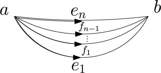
3 The Banana
$3$
-cell

Let
 $X_n$
be the
$X_n$
be the
 $n$
-faceted banana, with two
$n$
-faceted banana, with two
 $0$
-cells,
$0$
-cells,
 $n 1$
-cells,
$n 1$
-cells,
 $n$
bi-gon
$n$
bi-gon
 $2$
-cells, and one
$2$
-cells, and one
 $3$
-cell. The corresponding model will contain Lie algebra generators corresponding to each cell; denote them by
$3$
-cell. The corresponding model will contain Lie algebra generators corresponding to each cell; denote them by
 $a,b$
(grading
$a,b$
(grading
 $-1$
),
$-1$
),
 $e_i$
(
$e_i$
(
 $1\leq {}i\leq {}n$
, grading 0),
$1\leq {}i\leq {}n$
, grading 0),
 $f_i$
(
$f_i$
(
 $1\leq {}i\leq {}n$
, grading 1), and
$1\leq {}i\leq {}n$
, grading 1), and
 $h$
(grading 2), respectively. Here, the orientation on the
$h$
(grading 2), respectively. Here, the orientation on the
 $2$
-cell
$2$
-cell
 $f_i$
is chosen so that its geometric boundary is
$f_i$
is chosen so that its geometric boundary is
 ${\partial }_0f_i=e_{i}-e_{i+1}$
where
${\partial }_0f_i=e_{i}-e_{i+1}$
where
 $e_{n+1}\equiv {}e_1$
(indices modulo
$e_{n+1}\equiv {}e_1$
(indices modulo
 $n$
). The geometric boundary of
$n$
). The geometric boundary of
 $h$
is
$h$
is
 ${\partial }_0h=f_1+\cdots +f_n$
.
${\partial }_0h=f_1+\cdots +f_n$
.

3.1 Symmetries
The geometric symmetry group of the banana is
 $D_n\times {}\mathbb {Z}_2$
. The dihedral group is generated by the rotation by
$D_n\times {}\mathbb {Z}_2$
. The dihedral group is generated by the rotation by
 $\frac {2\pi }n$
around the axis
$\frac {2\pi }n$
around the axis
 $ab$
,
$ab$
,
 $$\begin{align*}\tau{\colon} e_i\longmapsto{}e_{i+1},\quad{}f_i\longmapsto{}f_{i+1},\quad{}a,b,h\ \text{fixed,}\end{align*}$$
and the reflection in the plane containing
 $e_n$
and the central axis of the banana,
$e_n$
and the central axis of the banana,
 $$\begin{align*}\sigma{\colon} a,b\ \text{fixed},\quad{}e_i\longmapsto{}e_{n-i}, \quad{}f_i\longmapsto{}-f_{n-i-1},\quad{}h\longmapsto-h,\end{align*}$$
while the further
 $\mathbb {Z}_2$
factor is generated by reflection in the plane equidistant from
$\mathbb {Z}_2$
factor is generated by reflection in the plane equidistant from
 $a$
and
$a$
and
 $b$
,
$b$
,
 $$\begin{align*}\iota: a\longleftrightarrow{}b,\quad{}e_i\longmapsto-e_i,\quad{} f_i\longmapsto-f_i,\quad{}h\longmapsto-h,\end{align*}$$
which commutes with both
 $\sigma $
and
$\sigma $
and
 $\tau $
. For some purposes we will restrict to the subgroup
$\tau $
. For some purposes we will restrict to the subgroup
 $D_n=\langle \sigma ,\tau \rangle $
of the symmetry group fixing the vertices.
$D_n=\langle \sigma ,\tau \rangle $
of the symmetry group fixing the vertices.
3.2
$0$
-,
$1$
-,
$2$
-cells


By the Leibniz rule, the differential
 ${\partial }$
is determined by its values on generators. On vertices,
${\partial }$
is determined by its values on generators. On vertices,
 ${\partial }$
is fixed by the Maurer–Cartan condition, namely,
${\partial }$
is fixed by the Maurer–Cartan condition, namely,
 $$ \begin{align} {\partial}{a}=-{\frac{1}{2}}[a,a],\qquad {\partial}{b}=-{\frac{1}{2}}[b,b]\>. \end{align} $$
On
 $1$
-cells,
$1$
-cells,
 ${\partial }$
is also unique (see Example 2.4):
${\partial }$
is also unique (see Example 2.4):
 $$ \begin{align} {\partial}{e_i}=\frac{E_i}{1-e^{E_i}}a+\frac{E_i}{1-e^{-E_i}}b =b-a+\tfrac12[a+b,e_i]+(\geq2\ \text{brackets}), \end{align} $$
where
 $E_i={\text {ad}}_{e_i}$
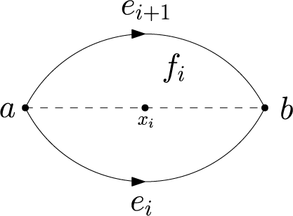
. The faces
$E_i={\text {ad}}_{e_i}$
. The faces
 $f_i$
are bi-gons, and we use the symmetric model of the bi-gon from [Reference Gadish, Griniasty and Lawrence6] in which
$f_i$
are bi-gons, and we use the symmetric model of the bi-gon from [Reference Gadish, Griniasty and Lawrence6] in which
 $$ \begin{align} {\partial}{}f_i={\text{BCH}}(-\tfrac12v_i,e_i,-e_{i+1},\tfrac12v_i)-[x_i,f_i] =e_i-e_{i+1}-\tfrac12[a+b,f_i]+\cdots \end{align} $$
so that
 $f_i$
is localised at its centre
$f_i$
is localised at its centre
 $$\begin{align*}x_i=u_{\frac12v_i}(a) =\tfrac12(a+b)+\frac1{16}[e_i+e_{i+1},b-a]+(\geq2\ \text{brackets}), \end{align*}$$
where
 $v_i$
is the centreline from
$v_i$
is the centreline from
 $a$
to
$a$
to
 $b$
given by the average
$b$
given by the average
 $$\begin{align*}v_i=\mu_2(e_i,e_{i+1})={\text{BCH}}(e_i,\tfrac12{\text{BCH}}(-e_i,e_{i+1})) =\tfrac12(e_i+e_{i+1})+(\geq2\ \text{brackets}) \end{align*}$$
in terms of the universal average
 $\mu _2$
of [Reference Lawrence and Siboni9].
$\mu _2$
of [Reference Lawrence and Siboni9].

3.3 Central Point of Banana
A totally symmetric point should be at the centre of the banana,
 $$\begin{align*}x=u_{\frac12v}(a) =\tfrac12(a+b)+\tfrac1{8n}\sum\limits_{i=1}^nE_i(b-a)+\cdots,\end{align*}$$
which is half way along a central diagonal of the banana from
 $a$
to
$a$
to
 $b$
, a path in the direction
$b$
, a path in the direction
 $v=\mu _n(e_1,\dots ,e_n)$
, the universal average of
$v=\mu _n(e_1,\dots ,e_n)$
, the universal average of
 $e_1,\dots ,e_n$
. The fact that
$e_1,\dots ,e_n$
. The fact that
 $x$
is invariant under
$x$
is invariant under
 $\sigma $
,
$\sigma $
,
 $\tau ,$
and
$\tau ,$
and
 $\iota $
follows from the total symmetry of
$\iota $
follows from the total symmetry of
 $\mu _n$
along with the fact that ([Reference Lawrence and Siboni9, Lemma 4.3])
$\mu _n$
along with the fact that ([Reference Lawrence and Siboni9, Lemma 4.3])
 $$\begin{align*}\mu_n(-e_1,\dots,-e_n)=-\mu_n(e_1,\dots,e_n).\end{align*}$$
The only freedom remaining in the model is the boundary of the
 $3$
-cell,
$3$
-cell,
 ${\partial }{h}\in {}A_1$
, which, to give a valid model of
${\partial }{h}\in {}A_1$
, which, to give a valid model of
 $X_n$
must be such that
$X_n$
must be such that
 ${\partial }^2(h)=0$
, while
${\partial }^2(h)=0$
, while
 $({\partial }{h})^{[0]}$
must coincide with the topological boundary
$({\partial }{h})^{[0]}$
must coincide with the topological boundary
 ${\partial }_0h=f_1+\cdots +f_n$
. The purpose of this section is to give a formula for
${\partial }_0h=f_1+\cdots +f_n$
. The purpose of this section is to give a formula for
 ${\partial }{h}$
that is invariant under the
${\partial }{h}$
that is invariant under the
 $D_n$
action of the symmetries of the banana fixing the vertices and in which
$D_n$
action of the symmetries of the banana fixing the vertices and in which
 $h$
is localised at a central point. In order to do this, we will first construct a model in which all the
$h$
is localised at a central point. In order to do this, we will first construct a model in which all the
 $2$
-cells and the
$2$
-cells and the
 $3$
-cell are localised at
$3$
-cell are localised at
 $a$
, and then twist using Lemma 2.12 to localise at a symmetric point.
$a$
, and then twist using Lemma 2.12 to localise at a symmetric point.
3.4 Model Localised at a
Since
 $f_i$
is localised at
$f_i$
is localised at
 $x_i$
,
$x_i$
,
 $f^{\prime }_i=\exp (\frac 12{\text {ad}}_{v_i})\cdot {}f_i$
is localised at
$f^{\prime }_i=\exp (\frac 12{\text {ad}}_{v_i})\cdot {}f_i$
is localised at
 $a$
; in particular,
$a$
; in particular,
 $$ \begin{align} {\partial}_a{}f^{\prime}_i={\text{BCH}}(e_i,-e_{i+1}). \end{align} $$
Similarly, set
 $h'=\exp (\frac 12{\text {ad}}_{v})\cdot {}h$
; by Lemma 2.12, a model in which
$h'=\exp (\frac 12{\text {ad}}_{v})\cdot {}h$
; by Lemma 2.12, a model in which
 $h$
is localised at
$h$
is localised at
 $x$
will have
$x$
will have
 $h'$
localised at
$h'$
localised at
 $a$
.
$a$
.
Lemma 3.1 A DGLA model of
 $X_n$
is defined by generators
$X_n$
is defined by generators
 $a,b,e_i,f^{\prime }_i,h^{\prime }$
, with the differential defined by (3.1), (3.2), and (3.4) along with
$a,b,e_i,f^{\prime }_i,h^{\prime }$
, with the differential defined by (3.1), (3.2), and (3.4) along with
 $$ \begin{align} {\partial}_ah^{\prime}=\sum\limits_{i=1}^nP_i\big({\text{BCH}}(E_1,-E_2),\dots,{\text{BCH}}(E_{n-1},-E_n)\big)\cdot{}f^{\prime}_i \end{align} $$
for any polynomials
 $P_i$
in
$P_i$
in
 $(n-1)$
non-commuting variables whose initial term is
$(n-1)$
non-commuting variables whose initial term is
 $1$
and satisfy the identity
$1$
and satisfy the identity
 $$ \begin{align} \sum\limits_{i=1}^{n-1}P_i({\text{ad}}_{x_1},\dots,{\text{ad}}_{x_{n-1}})&\cdot{}x_i \nonumber\\ &\quad=P_n({\text{ad}}_{x_1},\dots,{\text{ad}}_{x_{n-1}})\cdot{\text{BCH}}(x_1,\dots,x_{n-1}). \end{align} $$
In this model, the
 $3$
-cell and
$3$
-cell and
 $2$
-cells are all localised at
$2$
-cells are all localised at
 $a$
.
$a$
.
Proof It is apparent that the initial term of
 ${\partial }_ah'$
as defined by (3.5) is
${\partial }_ah'$
as defined by (3.5) is
 $\sum _{i=1}^nf^{\prime }_i,$
as required. It remains only to verify that
$\sum _{i=1}^nf^{\prime }_i,$
as required. It remains only to verify that
 ${\partial }_a^2h'=0$
, that is, that the RHS of (3.5) defines an element of
${\partial }_a^2h'=0$
, that is, that the RHS of (3.5) defines an element of
 $\ker {\partial }_a$
. For this, observe that since
$\ker {\partial }_a$
. For this, observe that since
 $u_{e_i}(a)=b$
, by Lemma 2.7,
$u_{e_i}(a)=b$
, by Lemma 2.7,
 $u_{{\text {BCH}}(e_i,-e_{i+1})}(a)=a,$
and so by Lemma 2.2,
$u_{{\text {BCH}}(e_i,-e_{i+1})}(a)=a,$
and so by Lemma 2.2,
 ${\text {BCH}}(e_i,-e_{i+1})\in \ker {\partial }_a$
. However, for
${\text {BCH}}(e_i,-e_{i+1})\in \ker {\partial }_a$
. However, for
 $y_1,\dots ,y_r\in \ker {\partial }_a$
of degree 0,
$y_1,\dots ,y_r\in \ker {\partial }_a$
of degree 0,
 $$\begin{align*}{\partial}_a[y_1,[y_2,\dots,[y_r,w]\cdots]]=[y_1,[y_2,\dots,[y_r,{\partial}{}w]\cdots]],\end{align*}$$
and so for any non-commuting polynomial
 $P$
,
$P$
,
 $P({\text {ad}}_{y_1},\dots ,{\text {ad}}_{y_r})$
commutes with
$P({\text {ad}}_{y_1},\dots ,{\text {ad}}_{y_r})$
commutes with
 ${\partial }_a$
. By Lemma 2.6(ii),
${\partial }_a$
. By Lemma 2.6(ii),
 ${\text {BCH}}({\text {ad}}_x,{\text {ad}}_y)={\text {ad}}_{{\text {BCH}}(x,y),}$
and it follows that
${\text {BCH}}({\text {ad}}_x,{\text {ad}}_y)={\text {ad}}_{{\text {BCH}}(x,y),}$
and it follows that
 $$ \begin{align*} &\partial_a \sum\limits_{i=1}^nP_i \big({\text{BCH}}(E_1,-E_2),\dots,{\text{BCH}}(E_{n-1},-E_n)\big)\cdot{}f^{\prime}_i\\ &\quad=\sum\limits_{i=1}^nP_i\big({\text{BCH}}(E_1,-E_2),\dots,{\text{BCH}}(E_{n-1},-E_n)\big)\cdot{}{\partial}_af^{\prime}_i\\ &\quad=\sum\limits_{i=1}^nP_i\big({\text{BCH}}(E_1,-E_2),\dots,{\text{BCH}}(E_{n-1},-E_n)\big)\cdot{}{\text{BCH}}(e_i,-e_{i+1})\\ &\quad=0, \end{align*} $$
where the second step follows from (3.4) and the third from (3.6) applied to
 $x_i={\text {BCH}}(e_i,-e_{i+1}),$
since
$x_i={\text {BCH}}(e_i,-e_{i+1}),$
since
 $-x_n={\text {BCH}}(x_1,\cdots ,x_{n-1})$
.▪
$-x_n={\text {BCH}}(x_1,\cdots ,x_{n-1})$
.▪
To see that the previous lemma’s constructions actually lead to a model of the
 $n$
-faceted banana, it remains only to show that
$n$
-faceted banana, it remains only to show that
 $P_1,\dots ,P_n$
exist with initial term 1 and satisfying identity (3.6). This follows immediately from Lemma 2.6(iii), even with
$P_1,\dots ,P_n$
exist with initial term 1 and satisfying identity (3.6). This follows immediately from Lemma 2.6(iii), even with
 $P_n\equiv 1$
; see the next subsection and (3.12). Indeed, there are many possible choices for
$P_n\equiv 1$
; see the next subsection and (3.12). Indeed, there are many possible choices for
 $P_1,\dots ,P_n$
.
$P_1,\dots ,P_n$
.
3.5 Model Localised at Central Point x
Twisting the model of Lemma 3.1 back so that the
 $2$
-cells are localised at their centres, and the
$2$
-cells are localised at their centres, and the
 $3$
-cell is localised at its centre
$3$
-cell is localised at its centre
 $x$
, we find the differential is given by (3.1), (3.2), and (3.3) along with
$x$
, we find the differential is given by (3.1), (3.2), and (3.3) along with
 $$ \begin{align} {\partial}_xh&=\nonumber\\&e^{-\frac12{\text{ad}}_v} \Big(\sum\limits_{i=1}^nP_i({\text{BCH}}(E_1,-E_2),\dots,{\text{BCH}}(E_{n-1},-E_n))\cdot{} e^{\frac12{\text{ad}}{v_i}}f_i\Big). \end{align} $$
The final requirement is that the model is symmetric under the action of
 $D_n$
; that is, it is invariant under
$D_n$
; that is, it is invariant under
 $\sigma $
,
$\sigma $
,
 $\tau $
. By the geometry and total symmetry of the bi-gon model, (3.1), (3.2), and (3.3) will be invariant under
$\tau $
. By the geometry and total symmetry of the bi-gon model, (3.1), (3.2), and (3.3) will be invariant under
 $\sigma $
,
$\sigma $
,
 $\tau ,$
and
$\tau ,$
and
 $\iota $
. Under
$\iota $
. Under
 $\tau $
,
$\tau $
,
 $x,h,v$
are fixed, while
$x,h,v$
are fixed, while
 $e_i\mapsto {}e_{i+1}$
,
$e_i\mapsto {}e_{i+1}$
,
 $f_i\mapsto {}f_{i+1}$
,
$f_i\mapsto {}f_{i+1}$
,
 $v_i\mapsto {}v_{i+1,}$
so (3.7) is invariant under
$v_i\mapsto {}v_{i+1,}$
so (3.7) is invariant under
 $\tau $
so long as
$\tau $
so long as
 $$ \begin{align*} P_i \big({\text{BCH}}(E_2,-E_3),\dots,{\text{BCH}}&(E_n,-E_1)\big)=\\ &P_{i+1}\big({\text{BCH}}(E_1,-E_2),\dots,{\text{BCH}}(E_{n-1},-E_n)\big), \end{align*} $$
which is ensured by
 $$ \begin{align} P_{i+1}(x_1,\dots,x_{n-1})=P_i\big(x_2,\dots,x_{n-1},-{\text{BCH}}(x_1,\dots,x_{n-1})\big). \end{align} $$
Under
 $\sigma $
,
$\sigma $
,
 $v,x$
are fixed,
$v,x$
are fixed,
 $e_i\mapsto {}e_{n-i}$
,
$e_i\mapsto {}e_{n-i}$
,
 $f_i\mapsto {}-f_{n-i-1}$
,
$f_i\mapsto {}-f_{n-i-1}$
,
 $v_i\mapsto {}v_{n-i-1,}$
while
$v_i\mapsto {}v_{n-i-1,}$
while
 $h$
changes sign. In order for (3.7) to be invariant under
$h$
changes sign. In order for (3.7) to be invariant under
 $\sigma $
, it is required that
$\sigma $
, it is required that
 $$ \begin{align*} P_i\big({\text{BCH}}(E_{n-1},-E_{n-2}),&\dots,{\text{BCH}}(E_1,-E_n)\big)=\\ &P_{n-i-1}\big({\text{BCH}}(E_1,-E_2),\dots,{\text{BCH}}(E_{n-1},-E_n)\big), \end{align*} $$
which is ensured by (3.8) along with
 $$ \begin{align} P_{n-i}(x_1,\dots,x_{n-1})=P_i(-x_{n-1},\dots,-x_1). \end{align} $$
Under
 $\iota $
, the quantities
$\iota $
, the quantities
 $e_i$
,
$e_i$
,
 $f_i$
,
$f_i$
,
 $v_i$
,
$v_i$
,
 $h,$
and
$h,$
and
 $v$
all change sign, while
$v$
all change sign, while
 $x$
is invariant, and so (3.7) is invariant under
$x$
is invariant, and so (3.7) is invariant under
 $\iota $
so long as
$\iota $
so long as
 $$ \begin{align} e^{\frac12{\text{ad}}_v}&P_i({\text{BCH}}(-E_1,E_2),\dots,{\text{BCH}}(-E_{n-1},E_n))e^{-\frac12{\text{ad}}_{v_i}}=\nonumber\\ &\qquad e^{-\frac12{\text{ad}}_v}P_{i}({\text{BCH}}(E_1,-E_2),\dots,{\text{BCH}}(E_{n-1},-E_n))e^{\frac12{\text{ad}}_{v_i}}, \end{align} $$
where
 $v_i=\mu _2(e_i,e_{i+1})$
and
$v_i=\mu _2(e_i,e_{i+1})$
and
 $v=\mu _n(e_1,\dots ,e_n)$
.
$v=\mu _n(e_1,\dots ,e_n)$
.
In conclusion, we have the following lemma.
Lemma 3.2 The completed DGLA with (free) Lie algebra generators
 $a,b,e_i,f_i,h$
and differential defined by (3.1), (3.2), (3.3), and (3.7) is a model for the
$a,b,e_i,f_i,h$
and differential defined by (3.1), (3.2), (3.3), and (3.7) is a model for the
 $n$
-faceted banana that is invariant under the geometric symmetries of the cell fixing the vertices, so long as the polynomials
$n$
-faceted banana that is invariant under the geometric symmetries of the cell fixing the vertices, so long as the polynomials
 $P_1,\dots ,P_n$
in
$P_1,\dots ,P_n$
in
 $(n-1)$
non-commuting variables, with initial term 1, satisfy identities (3.6), (3.8), and (3.9). It will be completely invariant under the symmetries of the
$(n-1)$
non-commuting variables, with initial term 1, satisfy identities (3.6), (3.8), and (3.9). It will be completely invariant under the symmetries of the
 $3$
-cell if, in addition, (3.10) holds.
$3$
-cell if, in addition, (3.10) holds.
By Lemma 2.6(i), we can write
 $$ \begin{align} BCH(x,y)=x+y+Q(X,Y)y, \end{align} $$
where
 $Q$
is a polynomial in two non-commuting variables whose lowest order terms are
$Q$
is a polynomial in two non-commuting variables whose lowest order terms are
 $\tfrac 12X+\tfrac 1{12}(X^2-YX)+\cdots $
. By Lemma 2.6(iii), iterating (3.11) gives
$\tfrac 12X+\tfrac 1{12}(X^2-YX)+\cdots $
. By Lemma 2.6(iii), iterating (3.11) gives
 $$\begin{align*}{\text{BCH}}(x_1,\dots,x_n)=\sum\limits_{i=1}^nx_i+\sum\limits_{i=2}^nQ({\text{BCH}}(X_1,\dots,X_{i-1}),X_i)x_i\end{align*}$$
so that
 $$ \begin{align}P_1=P_n=1,\quad{}P_i=1+Q \big({\text{BCH}}(X_1,\dots,X_{i-1}),X_i\big)\ \text{for } 1<i<n \end{align} $$
is a solution of (3.6). Note that (3.6) is a linear condition on
 $(P_1,\dots ,P_n)$
that is invariant under the action of cyclic permutation of the
$(P_1,\dots ,P_n)$
that is invariant under the action of cyclic permutation of the
 $P_i,$
while cyclically permuting the
$P_i,$
while cyclically permuting the
 $X_i$
(with
$X_i$
(with
 $X_n=-{\text {BCH}}(X_1,\dots ,X_{n-1})$
), as well as reversing the order of the
$X_n=-{\text {BCH}}(X_1,\dots ,X_{n-1})$
), as well as reversing the order of the
 $P_i$
while reversing the order and signs of the
$P_i$
while reversing the order and signs of the
 $x_i$
. That is, (3.6) is invariant under a dihedral group action, and so there exists an invariant solution (that will satisfy (3.8) and (3.9)) given by averaging the orbit of the solution (3.12) under the just described dihedral action. The result is that
$x_i$
. That is, (3.6) is invariant under a dihedral group action, and so there exists an invariant solution (that will satisfy (3.8) and (3.9)) given by averaging the orbit of the solution (3.12) under the just described dihedral action. The result is that
 $$ \begin{align*} P_i&=1+\tfrac1{2n}\!\!\!\!\sum\limits_{j=1+\delta_{in}}^{i-1}\!\!\!\!Q\big({\text{BCH}}(X_j,\dots,X_{i-1}),X_i\big) \\&\quad+\tfrac1{2n}\sum\limits_{j=i+1}^{n-1}\!\!\!Q\big(-{\text{BCH}}(X_i,\dots,X_j),X_i\big)\\ &\quad+\tfrac1{2n}\!\!\!\!\sum\limits_{j=1+\delta_{in}}^{i-1}\!\!\!\!Q\big({\text{BCH}}(X_j,\dots,X_i),-X_i\big) \\&\quad+\tfrac1{2n}\sum\limits_{j=i+1}^{n-1}\!\!\!Q\big(-{\text{BCH}}(X_{i+1},\dots,X_j),-X_i\big) \end{align*} $$
satisfies (3.6), (3.8), and (3.9). The coefficient of
 $f^{\prime }_i$
in
$f^{\prime }_i$
in
 ${\partial }_ah'$
from (3.5) is now
${\partial }_ah'$
from (3.5) is now
 $$ \begin{align*} P_i&\big({\text{BCH}}(E_1,-E_2),\dots,{\text{BCH}}(E_{n-1},-E_n)\big)\\ &=1+\tfrac1{2n}\sum\limits_{\substack{{j=1}\\{j\not=i,i+1}}}^{n} \Big(Q\big({\text{BCH}}(E_j,-E_i),{\text{BCH}}(E_i,-E_{i+1})\big)\\[-18pt] &\qquad\qquad\qquad\qquad+Q\big({\text{BCH}}(E_j,-E_{i+1}),{\text{BCH}}(E_{i+1},-E_i)\big )\Big). \end{align*} $$
Theorem 3.3 The completed DGLA with (free) Lie algebra generators
 $a,b,e_i,f_i,h$
and differential defined by (3.1), (3.2), (3.3) and
$a,b,e_i,f_i,h$
and differential defined by (3.1), (3.2), (3.3) and
 $$ \begin{align*} e^{\frac12{\text{ad}}_v}{\partial}_xh &= \sum\limits_{i=1}^nf^{\prime}_i+\tfrac1{2n} \sum\limits_{\substack{{i,j=1}\\{j\not=i,i+1}}}^n \Big(Q\big({\text{BCH}}(E_j,-E_i),{\text{BCH}}(E_i,-E_{i+1})\big)\\ &\quad+Q\big({\text{BCH}}(E_j,-E_{i+1}),{\text{BCH}}(E_{i+1},-E_i)\big )\Big)f^{\prime}_i \end{align*} $$
defines a model for the
 $n$
-faceted banana that is symmetric under the geometric symmetries of the cell fixing the vertices, where
$n$
-faceted banana that is symmetric under the geometric symmetries of the cell fixing the vertices, where
 $Q$
is defined by (3.11),
$Q$
is defined by (3.11),
 $f^{\prime }_i=e^{\frac 12{\text {ad}}_{v_i}}f_i$
,
$f^{\prime }_i=e^{\frac 12{\text {ad}}_{v_i}}f_i$
,
 $v_i=\mu _2(e_i,e_{i+1})$
,
$v_i=\mu _2(e_i,e_{i+1})$
,
 $v=\mu _n(x_1,\dots ,x_n),$
and
$v=\mu _n(x_1,\dots ,x_n),$
and
 $x=u_{\frac 12v}(a)$
. The
$x=u_{\frac 12v}(a)$
. The
 $3$
-cell is localised at
$3$
-cell is localised at
 $x$
in this model and the bi-gon
$x$
in this model and the bi-gon
 $2$
-cells are localised at their centres
$2$
-cells are localised at their centres
 $x_i=u_{\frac 12v_i}(a)$
.
$x_i=u_{\frac 12v_i}(a)$
.
Up to the first two non-trivial orders (in Lie brackets),
 $$ \begin{align*} v_i&=\tfrac12(e_i+e_{i+1})-\tfrac1{48}(E_i^2e_{i+1}+E_{i+1}^2e_i)+\cdots,\\ v&=\tfrac1n\sum\limits_ie_i-\tfrac1{12n^2}\sum\limits_{i\not-j}E_i^2e_j+\cdots,\\ x&=\tfrac12(a+b)+\tfrac1{8n}\sum\limits_i[e_i,b-a]+\cdots,\\ x_i&=\tfrac12(a+b)+\tfrac1{16}(E_i+E_{i+1})(b-a)+\cdots. \end{align*} $$
Meanwhile, up to second order (in Lie brackets) the differential is given by
 $$ \begin{align*} {\partial}{a}&=-\tfrac12[a,a],\qquad {\partial}{b}=-\tfrac12[b,b],\\[3pt] {\partial}{e_i}&=b-a+\tfrac12E_i(a+b)+\tfrac1{12}E_i^2(b-a)+\cdots,\\[3pt] {\partial}{}f_i&=e_i-e_{i+1}-\tfrac12[a+b,f_i]+\tfrac1{48}(E_{i+1}^2e_i-E_i^2e_{i+1}) +\tfrac1{16}[(E_i+E_{i+1})(a-b),f_i]+\cdots,\\[3pt] {\partial}{}h&=\sum\limits_if_i-\tfrac12[a+b,h]+\tfrac1{8n}\sum\limits_i[E_i(a-b),h]+\sum\limits_i \text{(quadratic in } E_j\text{'s)}f_i+\cdots. \end{align*} $$
Remark The particular solution of (3.6), (3.8) and (3.9) constructed above does not satisfy (3.10) and so the model described in Theorem 3.3 is not symmetric under the full symmetry group
 $D_n\times \mathbb {Z}_2$
, but only under the part fixing the vertices. In particular, it is not invariant under
$D_n\times \mathbb {Z}_2$
, but only under the part fixing the vertices. In particular, it is not invariant under
 $\iota $
, although such a model does exist. However, this model and the model it induces in Section 4 on the cube have sufficient symmetry for the applications in [Reference Lawrence, Ranade and Sullivan8], where cells will come with a preferred oriented main diagonal.
$\iota $
, although such a model does exist. However, this model and the model it induces in Section 4 on the cube have sufficient symmetry for the applications in [Reference Lawrence, Ranade and Sullivan8], where cells will come with a preferred oriented main diagonal.
4 A Model for an Arbitrary Polyhedral
$3$
-cell

Suppose that
 $X$
is an arbitrary polyhedral
$X$
is an arbitrary polyhedral
 $3$
-cell, with
$3$
-cell, with
 $n$
faces. Choose two vertices
$n$
faces. Choose two vertices
 $a$
and
$a$
and
 $b$
. Pick a shelling of the subdivision of the boundary, that is, a choice of
$b$
. Pick a shelling of the subdivision of the boundary, that is, a choice of
 $n$
non-self intersecting paths
$n$
non-self intersecting paths
 $\gamma _1,\dots ,\gamma _n$
each from a to b along edges of the polyhedron, in such a way that for each
$\gamma _1,\dots ,\gamma _n$
each from a to b along edges of the polyhedron, in such a way that for each
 $i=1,\dots ,n$
, the paths
$i=1,\dots ,n$
, the paths
 $\gamma _i$
and
$\gamma _i$
and
 $\gamma _{i+1}$
(with
$\gamma _{i+1}$
(with
 $\gamma _{n+1}\equiv \gamma _1$
) have common initial and final segments so that the intermediate segments together (one in reverse orientation) form the geometric boundary of the
$\gamma _{n+1}\equiv \gamma _1$
) have common initial and final segments so that the intermediate segments together (one in reverse orientation) form the geometric boundary of the
 $i$
-th face,
$i$
-th face,
 $g_i$
, of
$g_i$
, of
 $X$
. See the figure below; for each
$X$
. See the figure below; for each
 $i$
,
$i$
,
 $$\begin{align*}\gamma_i=\alpha_i\cup\delta_i\cup\beta_i,\quad\gamma_{i+1}=\alpha_i\cup\delta^{\prime}_i\cup\beta_i,\end{align*}$$
while
 $\delta _i\cup -\delta ^{\prime }_i={\partial }_0$
(
$\delta _i\cup -\delta ^{\prime }_i={\partial }_0$
(
 $i$
-th face) with matching orientation (faces oriented outwards). Here ,
$i$
-th face) with matching orientation (faces oriented outwards). Here ,
 $\delta _i$
and
$\delta _i$
and
 $\delta ^{\prime }_i$
share common initial and final points, say
$\delta ^{\prime }_i$
share common initial and final points, say
 $p_i$
and
$p_i$
and
 $q_i$
.
$q_i$
.

To construct a model
 $A(X)$
of
$A(X)$
of
 $X$
, first note that
$X$
, first note that
 $0$
-cells and
$0$
-cells and
 $1$
-cells have a unique description. For the
$1$
-cells have a unique description. For the
 $2$
-cells, pick a basepoint (say
$2$
-cells, pick a basepoint (say
 $p_i$
). In a model in which the
$p_i$
). In a model in which the
 $i$
-th cell
$i$
-th cell
 $f_i$
is localised at
$f_i$
is localised at
 $p_i:$
 $$\begin{align*}{\partial}_{p_i}f_i={\text{BCH}}(\delta_i,-\delta^{\prime}_i).\end{align*}$$
To determine a suitable expression for the differential of the
 $3$
-cell
$3$
-cell
 $h$
in
$h$
in
 $X$
, we decide to localise it at
$X$
, we decide to localise it at
 $a$
and then induce
$a$
and then induce
 ${\partial }{}h$
from the differential (3.5) on the
${\partial }{}h$
from the differential (3.5) on the
 $3$
-cell in the
$3$
-cell in the
 $n$
-faceted banana
$n$
-faceted banana
 $X_n$
using the natural DGLA map
$X_n$
using the natural DGLA map
 $A(X_n)\rightarrow {}A(X)$
in which
$A(X_n)\rightarrow {}A(X)$
in which
 $$ \begin{align*} a,b&\longmapsto{}a,b,\\ e_i&\longmapsto{}{\text{BCH}}(\gamma_i),\\ f^{\prime}_i&\longmapsto\exp({\text{BCH}}(\alpha_i))g_i,\\ h'&\longmapsto{}h, \end{align*} $$
using the notation of
 $f^{\prime }_i$
and
$f^{\prime }_i$
and
 $h'$
cells in
$h'$
cells in
 $X_n$
localised at
$X_n$
localised at
 $a$
as in (3.4) and (3.5) above. Thus, one can use in
$a$
as in (3.4) and (3.5) above. Thus, one can use in
 $A(X)$
:
$A(X)$
:
 $$\begin{align*}{\partial}_ah = \sum\limits_{i=1}^nP_i\big({\text{BCH}}({\text{ad}}_{\gamma_i},-{\text{ad}}_{\gamma_{i+1}}), \dots,{\text{BCH}}({\text{ad}}_{\gamma_{n-1}},-{\text{ad}}_{\gamma_n})\big)\cdot{}\exp\big({\text{BCH}}(\alpha_i)\big)g_i. \end{align*}$$
If it is desired to localise cells at symmetric central points in place of points on their boundary, then additional twists can be applied according to Lemma 2.12.
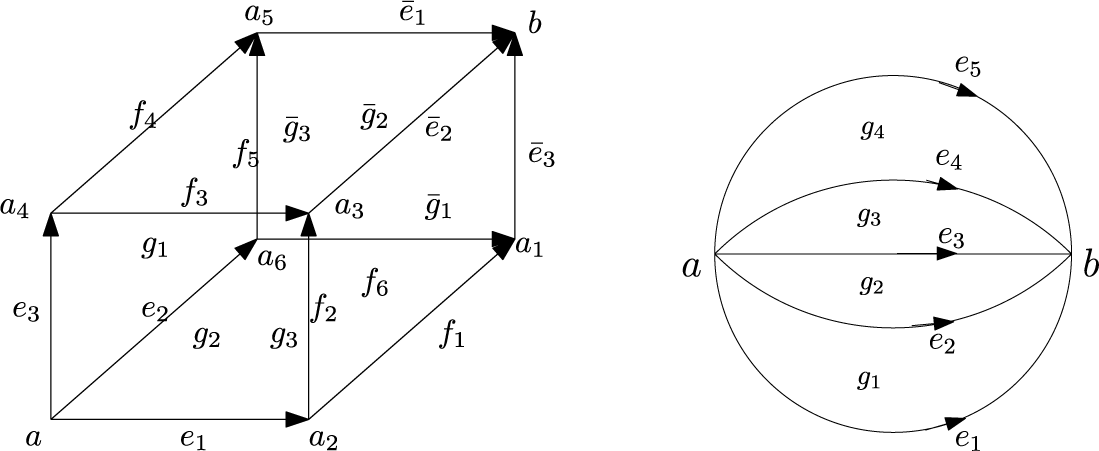
Example 4.1 We apply the above general argument to construct a model for the cube in which
 $2$
- and
$2$
- and
 $3$
-cells are localised at their centres. Denote a pair of antipodal vertices by
$3$
-cells are localised at their centres. Denote a pair of antipodal vertices by
 $a,b$
. If these vertices and their adjacent edges are removed from the skeleton of the cube, then a hexagon remains joining the six remaining vertices; label the vertices of this hexagon
$a,b$
. If these vertices and their adjacent edges are removed from the skeleton of the cube, then a hexagon remains joining the six remaining vertices; label the vertices of this hexagon
 $a_1,\dots ,a_6$
and the edges
$a_1,\dots ,a_6$
and the edges
 $f_1,\dots ,f_6$
(with
$f_1,\dots ,f_6$
(with
 $f_i$
joining
$f_i$
joining
 $a_i$
and
$a_i$
and
 $a_{i+1}$
modulo 6). Denote the edges adjacent to
$a_{i+1}$
modulo 6). Denote the edges adjacent to
 $a$
by
$a$
by
 $e_1,e_2,e_3$
and their opposite edges (adjacent to
$e_1,e_2,e_3$
and their opposite edges (adjacent to
 $b$
) by
$b$
) by
 $\overline {e}_1,\overline {e}_2,\overline {e}_3$
, respectively. Orient the edges so that those adjacent to
$\overline {e}_1,\overline {e}_2,\overline {e}_3$
, respectively. Orient the edges so that those adjacent to
 $a$
are oriented away from
$a$
are oriented away from
 $a$
and orient other edges so that parallel edges have matching orientation. The faces containing
$a$
and orient other edges so that parallel edges have matching orientation. The faces containing
 $a$
are labelled
$a$
are labelled
 $g_1,g_2,g_3$
and their opposite faces with a bar.
$g_1,g_2,g_3$
and their opposite faces with a bar.

 $x$
has
$x$
has
 ${\partial }{}x=-\tfrac 12[x,x],$
while the differential on all edges is also rigidly determined as in Example 2.4. The edge orientations give a partial ordering on the vertices, with
${\partial }{}x=-\tfrac 12[x,x],$
while the differential on all edges is also rigidly determined as in Example 2.4. The edge orientations give a partial ordering on the vertices, with
 $a$
as minimal element and
$a$
as minimal element and
 $b$
as maximal element. Each face similarly has a minimal and a maximal element that are diagonally opposite. The differential on faces of the cube is chosen so that they will be localised at their centre.
$b$
as maximal element. Each face similarly has a minimal and a maximal element that are diagonally opposite. The differential on faces of the cube is chosen so that they will be localised at their centre.
 $$\begin{align*}{\partial}_x{}g=\exp(-\tfrac12{\text{ad}}_v){\text{BCH}}(e_1,e_2,-e_3,-e_4),\end{align*}$$
where
 $x=u_{v/2}(a_1)$
is the centre point defined in terms of the centre diagonal
$x=u_{v/2}(a_1)$
is the centre point defined in terms of the centre diagonal
 $$\begin{align*}v=\mu_2\big({\text{BCH}}(e_1,e_2),{\text{BCH}}(e_4,e_3)\big).\end{align*}$$
The formula for the cube is induced from a symmetric model of a
 $6$
-faceted banana, by mapping the edges of
$6$
-faceted banana, by mapping the edges of
 $X_6$
to
$X_6$
to
 ${\text {BCH}}$
of the 6 maximal chains from
${\text {BCH}}$
of the 6 maximal chains from
 $a$
to
$a$
to
 $b$
on the cube, while mapping the faces
$b$
on the cube, while mapping the faces
 $f_i$
(based at their centres) to the conjugations of the corresponding faces of the cube,
$f_i$
(based at their centres) to the conjugations of the corresponding faces of the cube,
 $\exp (-V_i)g_i$
, where
$\exp (-V_i)g_i$
, where
 $v_i$
is a zero graded element that flows the centre
$v_i$
is a zero graded element that flows the centre
 $x_i$
of the
$x_i$
of the
 $i$
-th face of the cube to the centre of the corresponding bi-gon bounded by two maximal chains (thus changing the point at which it is localised). Here, by the centre of a square, we mean the centre point as in the formulae for
$i$
-th face of the cube to the centre of the corresponding bi-gon bounded by two maximal chains (thus changing the point at which it is localised). Here, by the centre of a square, we mean the centre point as in the formulae for
 ${\partial }$
of a square above. Up to terms with only one bracket (which are all that affect the result of
${\partial }$
of a square above. Up to terms with only one bracket (which are all that affect the result of
 $\exp (-V_i)g_i$
up to two brackets), the
$\exp (-V_i)g_i$
up to two brackets), the
 $v$
’s for the squares
$v$
’s for the squares
 $g_1$
,
$g_1$
,
 $g_2$
,
$g_2$
,
 $g_3$
,
$g_3$
,
 $\overline {g}_1$
,
$\overline {g}_1$
,
 $\overline {g}_2$
,
$\overline {g}_2$
,
 $\overline {g}_3$
are
$\overline {g}_3$
are
 $\frac 12\overline {e}_1$
,
$\frac 12\overline {e}_1$
,
 $\frac 12\overline {e_2}$
,
$\frac 12\overline {e_2}$
,
 $\frac 12\overline {e}_3$
,
$\frac 12\overline {e}_3$
,
 $-\frac 12e_1$
,
$-\frac 12e_1$
,
 $-\frac 12e_2$
,
$-\frac 12e_2$
,
 $-\frac 12e_3$
, respectively. That is,
$-\frac 12e_3$
, respectively. That is,
 $A(X_6)\rightarrow {}A(\text {cube})$
is given on edges by
$A(X_6)\rightarrow {}A(\text {cube})$
is given on edges by
 $$ \begin{align*} e_1&\longmapsto{\text{BCH}}(e_3,f_4,\overline{e}_1),\\ e_2&\longmapsto{\text{BCH}}(e_2,f_5,\overline{e}_1),\\ e_3&\longmapsto{\text{BCH}}(e_2,f_6,\overline{e}_3),\\ e_4&\longmapsto{\text{BCH}}(e_1,f_1,\overline{e}_3),\\ e_5&\longmapsto{\text{BCH}}(e_1,f_2,\overline{e}_2),\\ e_6&\longmapsto{\text{BCH}}(e_3,f_3,\overline{e}_2), \end{align*} $$
and on faces by
 $$ \begin{align*} g_1&\longmapsto-\exp(-\tfrac12\overline{E}_1){g}_1+(\geq2\text{ brackets}),\\ g_2&\longmapsto-\exp(\tfrac12E_2)\overline{g}_2+(\geq2\text{ brackets}),\\ g_3&\longmapsto-\exp(-\tfrac12\overline{E}_3){g}_3+(\geq2\text{ brackets}),\\ g_4&\longmapsto\exp(\tfrac12E_1)\overline{g}_1+(\geq2\text{ brackets}),\\ g_5&\longmapsto\exp(-\tfrac12\overline{E}_2){g}_2+(\geq2\text{ brackets}),\\ g_6&\longmapsto\exp(\tfrac12E_3)\overline{g}_3+(\geq2\text{ brackets}). \end{align*} $$
Up to one Lie bracket in
 $A(X_6),$
 $$\begin{align*}{\partial}{}h=\sum\limits_ig_i-\tfrac12[a+b,h]+(\geq2\text{ brackets}),\end{align*}$$
which transforms on the cube to
 $$ \begin{align*} {\partial}{}h &= \overline{g}_1+g_2+\overline{g}_3-g_1-\overline{g}_2-g_3-\tfrac12[a+b,h]\\ & \quad + \tfrac12(E_3\overline{g}_3-\overline{E}_2g_2+E_1\overline{g}_1+\overline{E}_3g_3-E_2\overline{g}_2+\overline{E}_1g_1)+(\geq2\text{ brackets}). \end{align*} $$
The model of the cube so obtained will be symmetric under symmetries that fix the diagonal
 $ab$
.
$ab$
.
Remark Notice that the structure of the differential for
 $3$
-cells is essentially simpler than that for
$3$
-cells is essentially simpler than that for
 $2$
-cells, having a linear dependence on its codimension one boundary sub-cells. Thus, in (3.5), the dependence of
$2$
-cells, having a linear dependence on its codimension one boundary sub-cells. Thus, in (3.5), the dependence of
 ${\partial }_ah'$
upon
${\partial }_ah'$
upon
 $f_i$
is linear. This is not true one dimension lower, where the dependence in (3.4) of
$f_i$
is linear. This is not true one dimension lower, where the dependence in (3.4) of
 ${\partial }_af^{\prime }_i$
on its boundary cells
${\partial }_af^{\prime }_i$
on its boundary cells
 $e_i$
and
$e_i$
and
 $e_{i+1}$
is highly non-linear (through
$e_{i+1}$
is highly non-linear (through
 ${\text {BCH}}$
).
${\text {BCH}}$
).
Remark The functorial nature of the construction of
 $A(X)$
from
$A(X)$
from
 $X$
means that under a subdivision, there should be a corresponding DGLA map. The subdivision map for the interval (or 1-skeleta) is generated by
$X$
means that under a subdivision, there should be a corresponding DGLA map. The subdivision map for the interval (or 1-skeleta) is generated by
 ${\text {BCH}}$
(see [Reference Lawrence and Sullivan10]), and for this reason, the differential on a
${\text {BCH}}$
(see [Reference Lawrence and Sullivan10]), and for this reason, the differential on a
 $2$
-cell (in its simplest form) is the
$2$
-cell (in its simplest form) is the
 ${\text {BCH}}$
of its boundary (see (3.4)). Similarly, the subdivision map for a
${\text {BCH}}$
of its boundary (see (3.4)). Similarly, the subdivision map for a
 $2$
-cell (say splitting a bi-gon into two bi-gons) will be linear, and the difference between the two sides gives an expression for the differential on a
$2$
-cell (say splitting a bi-gon into two bi-gons) will be linear, and the difference between the two sides gives an expression for the differential on a
 $3$
-cell as in (3.5). This same story should continue in higher dimensions (all dimensions
$3$
-cell as in (3.5). This same story should continue in higher dimensions (all dimensions
 $>2$
will have a linear form).
$>2$
will have a linear form).
