2. Describing injection-driven fragmentation cascades

We consider the population density function $n(a,\boldsymbol {x},t)$ (dimension $L^{-4}$) where $n(a,\boldsymbol {x},t)\delta a \delta \boldsymbol {x}$ is the number of bubbles of radius $a< a' < a + \delta a$ in a volume $\delta \boldsymbol {x}$ around a specified location $\boldsymbol {x}$ at time $t$. A Boltzmann-type population balance model describes the evolution of $n$ (Williams Reference Williams1985, chap. 11):

(2.1)\begin{equation} {\partial n}/{\partial t} + \boldsymbol{\nabla}\boldsymbol{\cdot}(\bar{\boldsymbol{v}} n)= s_d+s_b+s_c , \end{equation}

where $\bar {\boldsymbol {v}}$ is the mean velocity of bubbles of the given radii, and $s_d$, $s_b$ and $s_c$ are respectively the movement of air between bubble sizes due to dissolution, fragmentation and coalescence. For locally uniform flows, integrating $n(a,\boldsymbol {x},t)$ over the domain, we define the bulk bubble-size distribution $N(a,t)$, of dimension $L^{-1}$. Integrating $s_b$ over the domain yields the bulk fragmentation contribution $S_b$:

(2.2)\begin{equation} S_b(a,t) ={-} \varOmega(a) N(a,t) + \int_a^\infty m(a') f(a;a') \varOmega(a') N(a',t) \,\mathrm{d}a', \end{equation}

where $m(a')$ is the number of daughter bubbles created during the breakup of a parent of radius $a'$ and $f(a;a')$ is the radius-based probability density function (p.d.f.) describing the radius $a$ of daughter bubbles created by that breakup (Liao & Lucas Reference Liao and Lucas2009; Martínez-Bazán et al. Reference Martínez-Bazán, Rodríguez-Rodríguez, Deane, Montaes and Lasheras2010).

For simplicity, we focus on the relationship between entrainment and fragmentation, ignoring coalescence, dissolution and degassing. Thus,

(2.3)\begin{equation} {\partial N}/{\partial t}(a,t) = S_b(a,t)+I(a) \end{equation}

defines the population balance model for an injection-driven fragmentation cascade with $I(a)$ the (steady) inflow of bubbles into the domain due to entrainment. Our interest is for $a>a_H$, and, as modelled, $N(a,t)$ depends only on scales larger than $a$; thus, sub-Hinze-scale mechanisms can be ignored.

2.1. A simple population balance model (S-PBM) for fragmentation cascades

An analytic solution to $N(a,t)$ requires a simplified description of $S_b$. To satisfy volume conservation and the definition of a p.d.f., $f(a';a)$ must satisfy the following (Martínez-Bazán et al. Reference Martínez-Bazán, Rodríguez-Rodríguez, Deane, Montaes and Lasheras2010):

(2.4a,b)\begin{equation} m(a) \int_0^a (a'/a)^3 f(a';a) \,\mathrm{d}a' = 1, \quad \int_0^a f(a';a) \,\mathrm{d}a' = 1 . \end{equation}

For simplicity, we assume a bubble breaks up into $m$ (independent of $a$) identical bubbles (Garrett et al. Reference Garrett, Li and Farmer2000). Satisfying (2.4a,b) produces the identical daughter distribution (Valentas, Bilous & Amundson Reference Valentas, Bilous and Amundson1966)

(2.5)\begin{equation} f(a';a) = \delta(a'-a m^{{-}1/3}) . \end{equation}

Equation (2.5) makes analytic evaluation in §§ 2.2 and 3.1 possible. §§ 3.2 and 4 consider more realistic daughter distributions from literature. Combining (2.2) and (2.5), and upon integration with a change of variable for the delta function, we obtain

(2.6)\begin{equation} S_b(a,t) ={-} \varOmega(a) N(a,t) + m^{1/3} [ m \varOmega( m^{1/3} a) N( m^{1/3} a,t) ] . \end{equation}

Using (1.1) and (2.6), we simplify (2.3) and define the simple population balance model (S-PBM) as

(2.7)\begin{equation} {\partial N^*}/{\partial t^*}(a^*,t^*) = {a^*}^{{-}2/3}[{-}N^*(a^*,t^*)+m^{10/9} N^*(m^{1/3} a^*,t^*)] + I^*(a^*), \end{equation}

where $\cdot ^*$ denotes nondimensionalisation using the characteristic bubble radius $L=a_{max}$ and time $T=\varOmega (a_{max})^{-1}$.

2.2. Scale-invariant solutions to S-PBM

We consider solutions to (2.7) where $N^*(a^*,t^*)={a^*}^\beta g(t^*)$ for all $a\in (0,\infty )$, defining $g(t^*)$ to be only a function of time. Substituting into (2.7) gives

(2.8)\begin{equation} {\mathrm{d} g}/{\mathrm{d} t^*} = g {a^*}^{{-}2/3} ({-}1 + m^{\beta/3+10/9}) + {a^*}^{-\beta} I^*(a^*). \end{equation}

For $g(t^*)$ to be independent of $a^*$ and injection to be non-trivial, $I^*$ must also be scale-invariant: $I^*(a)= h {a^*}^\gamma$ for all $a\in (0,\infty )$, where $h$ is a constant, and the power-law slope is $\gamma$. There are only two admissible solutions for the form of $N^*$ we consider. The first is a transient solution in which $\beta =\gamma =-10/3$ and $\mathrm {d} g/\mathrm {d} t^*=h$, resulting in $S_b=0$. This ($S_b=0$) is equivalent to the condition imposed by Garrett et al. (Reference Garrett, Li and Farmer2000) to represent an equilibrium for their fragmentation cascade. The second solution is a steady-state solution in which $\beta =\gamma +2/3$ and $\mathrm {d} g/\mathrm {d} t^*=0$. Both admissible solutions have physical limitations. To describe the commonly observed $\beta =-10/3$, they would suggest $\gamma =-10/3$ or $\gamma =-4$; however, $\gamma \ge -4$ implies an infinite rate of volume injection.

3. Equilibrium solutions for cutoff spectral injection

Based on the mechanistic energy argument by Yu et al. (Reference Yu, Hendrickson and Yue2020) and § 2.2, we assume an entrainment size distribution described by a power law of slope $\gamma$. To ensure a finite rate of volume injection, we introduce a cutoff radius $a_{max}$ above which there is no bubble injection. In addition to ensuring finite injected volume if $\gamma \ge -4$, physical limits of a flow will necessarily impose some $a_{max}$. For example, Yu et al. (Reference Yu, Hendrickson and Yue2020) proposed an $a_{max}$ for entraining free-surface turbulence based on bubble Froude number. The cutoff spectral injection model (SIM) is thus

(3.1)\begin{equation} I^* = h (a^*)^\gamma \mathcal{H}(1-a^*), \end{equation}

where $\mathcal {H}$ is the Heaviside step function. Note that (3.1) is a generalization of Garrett et al. (Reference Garrett, Li and Farmer2000), which corresponds to $\gamma \rightarrow \infty$ (all bubbles injected at $a=a_{max}$). In § 4, we show that under SIM, $N(a,t)$ approaches an equilibrium $N_{eq}(a)$ in a time scale given by $\tau _c$.

SIM allows us to define a new global condition for equilibrium: the volume flux of air injected as bubbles larger than $a$ must be equal to the volume flux of air from bubbles larger than $a$ to bubbles smaller than $a$ due to fragmentation; i.e.,

(3.2)\begin{equation} \int_{a^*}^\infty I^*(r) r^3 \,\mathrm{d}r = \int_{a^*}^\infty N_{eq}^*(r) \varOmega^*(r) m \int_0^{a^*} {r'}^3 f^*(r';r) \,\mathrm{d}r' \,\mathrm{d}r, \end{equation}

where the integration variables $r$ and $r'$ are dimensionless (scaled by $a_{max}$).

3.1. Local power-law slope of the equilibrium bulk bubble-size distribution

Rather than assuming a strict power-law relationship as in § 2.2, we allow the power-law slope to vary continuously with radius, described by $\tilde {\beta }(a^*)$. We define a local approximation

(3.3)\begin{equation} N_{eq}^*(r)\approx\tilde{g}_{eq}(a^*)r^{\tilde{\beta}_{eq}(a^*)} \quad \text{for } r\sim a^* . \end{equation}

Applying this as well as (1.1) and (3.1) to (3.2) produces

(3.4)\begin{equation} h \int_{a^*}^1 r^{\gamma+3} \,\mathrm{d}r = \tilde{g}_{eq}(a^*) \int_{a^*}^1 {r}^{\tilde{\beta}_{eq}(a^*)-2/3} m \int_0^{a^*} {r'}^3 f^*(r';r) \,\mathrm{d}r'\,\mathrm{d}r. \end{equation}

We note that for ${a^*}^{\gamma +4}\ll 1$, the left side of (3.4) approaches the (non-dimensionalised) steady volumetric flow rate of air being injected, $Q^*$. As $\tilde {g}_{eq}(a^*)$ is a measure of the magnitude of $N_{eq}^*(a^*)$, and it will be shown in § 4 that $\tilde {g}_{eq}(a^*\ll 1)$ is independent of $a^*$, we recover the linear proportionality between $N_{eq}(a)$ and $Q$ given by (1.2) for $a\ll a_{max}$.

To further simplify (3.4), we assume identical fragmentation (2.5). Noting that in this case the inner integral on the right side of (3.4) is only non-zero for $r < a^* m^{1/3}$, we change the upper limit of integration on the outer integral to $a^* m^{1/3}$ and obtain

(3.5)\begin{equation} h (\gamma+4)^{{-}1} [1-{a^*}^{\gamma+4}]= \tilde{g}_{eq}(a^*) \frac{{a^*}^{\tilde{\beta}_{eq}(a^*)+10/3}}{\tilde{\beta}_{eq}(a^*)+10/3} [{m}^{\tilde{\beta}_{eq}(a^*)/3+10/9}-1]. \end{equation}

Applying the local equilibrium condition $\partial N_{eq}(a) / \partial t =0$, (2.7) gives

(3.6)\begin{equation} {a^*}^{{-}2/3}[ m^{10/9} N_{eq}^*( a^* m^{1/3})-N_{eq}^*(a^*)] + h {a^*}^{\gamma} = 0 . \end{equation}

Using the local approximation (3.3) about $a^*$ to approximate $N_{eq}^*(a^* m^{1/3})$ gives

(3.7)\begin{equation} \tilde{g}_{eq}(a^*) {a^*}^{\tilde{\beta}_{eq}(a^*)-2/3}( m^{\tilde{\beta}_{eq}(a^*)/3+10/9}-1) + h {a^*}^{\gamma} = 0 . \end{equation}

Combining (3.5) and (3.7), we determine the relationship between $\tilde {\beta }_{eq}(a)$ and the injection power-law slope $\gamma$:

(3.8)\begin{equation} \tilde{\beta}_{eq}(a) = \frac{\gamma+4}{1-(a_{max}/a)^{\gamma+4}} - 10/3 . \end{equation}

We note that as $a\rightarrow a_{max}$, $\tilde {\beta }_{eq}(a)$ becomes more negative; the equilibrium slope becomes steeper for the largest bubbles. We revisit this point in § 5.

When $a_H \ll a_{max}$, most of the bubble-size distribution will follow a single power law $\beta =\tilde {\beta }_{eq}(a \ll a_{max})$. There are two distinct regimes, which are similar to those in § 2.2. The weak injection regime ($\gamma \ge -4$) has injected volume concentrated at large bubbles, and as a result the fragmentation term dominates the injection term of (2.3) at equilibrium. Here, the equilibrium slope is $\tilde {\beta }_{eq}(a \ll a_{max})=-10/3$, independent of $\gamma$. We note that we can recover Garrett et al. (Reference Garrett, Li and Farmer2000): when $\gamma =\infty$, $\tilde {\beta }_{eq}(a)=-10/3$ for all $a<a_{max}$. The strong injection regime ($\gamma < -4$) has injected volume concentrated at small bubbles, and the injection term dominates (2.3) at equilibrium. Yet fragmentation still modifies the equilibrium slope and $\tilde {\beta }_{eq}(a \ll a_{max})=\gamma +2/3$. In both regimes, $\tilde {\beta }_{eq}(a)\le -10/3$, making it the upper limit of the power-law slope. We conclude by noting that in the weak regime, because $\tilde {\beta }_{eq}(a)$ is independent of $\gamma$, the equilibrium bubble-size distribution cannot be used to infer information on the underlying entrainment distribution.

3.2. The influence of fragmentation daughter distribution models

We consider here the effect of daughter distributions more realistic than the identical distribution used in § 3.1. Phenomenological daughter distributions are typically categorised as bell-shaped, U-shaped or M-shaped (Liao & Lucas Reference Liao and Lucas2009). We consider a binary-fragmentation ($m=2$) daughter distribution from each category and a daughter distribution proposed by Diemer & Olson (Reference Diemer and Olson2002) for $m\ne 2$. We assume ${\textit {We}}=\infty$, so there is no minimum daughter-bubble radius and the daughter distributions become scale-invariant. We describe these daughter distributions using the volume-based p.d.f. $f_V^*(V^*)$ based on the relative volume $V^*=(a'/a)^3$, which is related to the radius-based p.d.f. by $a f(a';a)= 3 {V^*}^{2/3} f_V^*(V^*)$ (Martínez-Bazán et al. Reference Martínez-Bazán, Rodríguez-Rodríguez, Deane, Montaes and Lasheras2010). Table 1 gives the volume-based p.d.f. for each daughter distribution considered.

Table 1. Volume-based p.d.f.s, $f_V^*(V^*)$, of daughter distributions used in simulations and corresponding time scaling constant $C_f$ calculated using (4.4). Note that a constant to ensure $\int f_V^*(V^*)\,\mathrm {d}V^*=1$ is omitted for brevity.

To confirm the validity of (3.8) for general daughter distributions, we perform two types of simulations over a broad range of $\gamma$ and $a_{max}/a$: (a) direct numerical simulations of the S-PBM (2.7); and (b) Monte Carlo (MC) simulations where fragmentation following (1.1) and injection following SIM are modelled as Poisson processes over each fixed ${\rm \Delta} t$. Direct simulation of (2.7) is inexpensive because it is deterministic, but it is applicable only for identical daughter distributions (case A in table 1 for $m=2$). In these simulations, discretisation of radius is done on a logarithmic scale and Heun's method is used for time marching. MC simulations are computationally more expensive, but capture the stochastic nature of fragmentation and entrainment and are applicable for general daughter distributions. MC simulations are performed for cases in table 1 where the daughter bubbles from each fragmentation event are chosen using random sampling of the respective distributions. Due to the power-law nature of bubble-size distributions, the simulated distributions are averaged over logarithmic intervals based on $m^{1/3}$:

(3.9a)\begin{gather} {\langle{N(a)}\rangle}_m = ( a (m^{1/3} - 1) )^{{-}1} \int_a^{a\,m^{1/3}} N(a') \, \mathrm{d}a', \end{gather}

(3.9b)\begin{gather}{\langle{\tilde{\beta}(a)}\rangle}_m = 3 \ln( {{\langle{N(a)}\rangle}_m}/{{\langle{N(a\,m^{{-}1/3})}\rangle}_m} ) /\ln(m). \end{gather}

We establish convergence for both simulation types with $\varOmega (a) {\rm \Delta} t = 1/100$ and $30$ bins per $m^{1/3}$ interval for the radius discretisation of S-PBM. The results of the S-PBM and MC simulations are compared to (3.8) in figure 1 and show good agreement. These simulations demonstrate that the equilibrium slope predicted by (3.8), although based on the simplifying assumption of identical fragmentation, is, in fact, applicable to general daughter distributions. This is consistent with the observation by Qi et al. (Reference Qi, Mohammad Masuk and Ni2020) that the choice of daughter distribution has no effect on the equilibrium power-law slope for fragmentation cascades.

Figure 1. Comparison of equilibrium local power-law slopes resulting from SIM with a range of injection power-law slopes $\gamma$, as modelled by (3.8) (—–); case A ($\bullet$); case B ($+$, blue); case C ($\times$, yellow); case D ($\square$, red); case E ($\circ$, green); case F ($\circ$, purple). Case A is calculated using direct numerical simulations, cases B–F using MC simulations. The value of $a_{max}/a$ for the reported ${\langle {\tilde {\beta }_{eq}(a)}\rangle }_m$ is indicated below each data set. For the MC simulations, the inset shows the equilibrium bubble-size distributions for $\gamma =-10/3$ compared to $\propto a^{-10/3}$ (- - - -).

4. Time scale of convergence to the equilibrium distribution

We investigate the convergence time $\tau$ such that $N(a,t>t_0+\tau )\approx N_{eq}(a)$, where $N(a,t_0)=0$. First, we revisit the global equilibrium condition (3.4). Rewriting it in terms of $f_V^*$, we have

(4.1)\begin{equation} h \int_{a^*}^1 r^{\gamma+3}\,\mathrm{d}r = \tilde{g}_{eq}(a^*) \frac{m}{3} {a^*}^{\tilde{\beta}_{eq}(a^*)+10/3}\ \int_{{a^*}^3}^1 {u}^{-\tilde{\beta}_{eq}(a^*)/3-19/9} \int_0^{u} v f_V^*(v) \,\mathrm{d}v\,\mathrm{d}u . \end{equation}

For weak injection, we consider the limiting case $a^*\rightarrow 0$. By (3.8), $\tilde {\beta }_{eq}(a^*)=-10/3$ and we can simplify (4.1):

(4.2)\begin{equation} \frac{h}{\gamma+4} = \tilde{g}_{eq}(a^*\ll1) \frac{m}{3}\ \int_{0}^1 {u}^{{-}1} \int_0^{u} v f_V^*(v) \,\mathrm{d}v\,\mathrm{d}u . \end{equation}

Rearranging (4.2), we define a new constant $C_f$ to quantify the effect of $f_V^*$ on $\tilde {g}_{eq}$ and scale $C_f$ so that for an identical daughter distribution, (2.5), it has a value of unity:

(4.3a,b)\begin{equation} \tilde{g}_{eq}(a^*\ll1)= \frac{3}{\ln(m) } \frac{h}{\gamma+4} C_f; \quad C_f=\frac{\ln(m)/m}{\displaystyle \int_{0}^1 \int_0^{1} u w f_V^*(u w) \,\mathrm{d}w\,\mathrm{d}u} . \end{equation}

Table 1 shows the numerically calculated values of $C_f$.

We write the varying power-law slope description of the bubble-size distribution $N_{eq}$ from § 3.1, now as a function of time: $N^*(a^*,t^*)\approx \tilde {g}(a^*,t^*){a^*}^{\tilde {\beta }(a^*,t^*)}$. With the dependence on $a^*$ omitted for clarity, $\tilde {g}(t)$ has a Taylor approximation to first order: $\hat {g}(t) = \tilde {g}(t_0) + (t-t_0) \tilde {g}^{\prime }(t_0)$. Using (2.3) and $\tilde {g}(t_0)=0$, we obtain $\tilde {g}^{\prime }(t_0)=h {a^*}^{\gamma -\tilde {\beta }(a^*,t_0)}$. Note that we neglected the time dependence of $\tilde {\beta }(a^*,t)$ (cf. figure 2), making $\hat {g}(t)$ a poor description of the general evolution of $N^*(a^*,t^*)$. However for the special case $\gamma =-10/3$ and $a^*\ll 1$, $\tilde {\beta }(a^*,t)=\gamma$ and we can define a critical time $\tau _c$ such that $\hat {g}(t_0+\tau _c)=\tilde {g}_{eq}(a^*\ll 1)$:

(4.4)\begin{equation} \tau_c = (9/2)(\ln m)^{{-}1}({C_f}/{C_\varOmega}) \varepsilon^{{-}1/3} {a_{max}}^{2/3} . \end{equation}

Despite the special case used in deriving (4.4), numerical simulations of S-PBM and MC simulations of realistic daughter distributions (cf. § 3.2) show that $\tau _c$ provides a general time scaling, with equilibrium reached at $\tau \approx 2\tau _c$ for weak injection and $\tau \lesssim \tau _c$ for strong injection. Figure 2 shows results from simulations of $a_{max}/a=3$ and $a_{max}/a=10$. The S-PBM simulations of larger $a_{max}/a$ (not shown) demonstrate similar behaviour for weak injection, with $\tau /\tau _c$ becoming smaller for strong injection. Figure 2 provides a direct means to validate (4.4) experimentally if the relevant underlying parameters are known or can be measured; and an indirect means to deduce the shape of the daughter distribution if the evolution of the bubble-size distributions can be quantitatively obtained.

Figure 2. Evolution of bubble-size distribution $N$ (b and d) and local power-law slope $\tilde {\beta }$ (a and c) as measured at $a_{max}/a=3$ (a and b) and $a_{max}/a=10$ (c and d). Numerical simulations of case A (- - - -) and MC simulations (——–) of cases B–F (cf. table 1). Colours based on $\gamma$: green, $\gamma =-5$; red, $\gamma =-10/3$; blue, $\gamma =-5/3$; magenta, $\gamma =0$; black, $\gamma =\infty$ (single-radius injection). Note that $\tilde {\beta }(t\ll \tau _c)$ is not reported for MC simulations of $\gamma =\infty$ due to significant noise.

We make two comments on (4.4). First, although we consider power-law injection rather than single-radius injection, the dependence of $\tau _c$ on $m$ (disregarding $C_f$) is similar to the equation (1.3) proposed by Deike et al. (Reference Deike, Melville and Popinet2016). For ${\textit {We}}=\infty$ and small $m$, $c_{\infty ,m}=1-1/(m^{-1/3}-1)$ $\sim$ $(9/2)(\ln m)^{-1}$. Considering a more typical $a_H/a_{max}\approx 10$, for binary breakup ($m=2$) the coefficient for $\tau _c$ in (4.4) is $(9/2)(\ln 2)^{-1}\approx 6.5$, and for tertiary breakup ($m=3$) the coefficient is $(9/2)(\ln 3)^{-1}\approx 4.1$. These values compare well with those obtained from the simulations of Deike et al. (Reference Deike, Melville and Popinet2016). Second, the value of $C_f$ provides a new quantification of the dependence of $\tau _c$ on $f_V^*$ first described by Qi et al. (Reference Qi, Mohammad Masuk and Ni2020): the closer a daughter distribution is to identical fragmentation, the faster the convergence to equilibrium. Through $C_f$, observed convergence times now provide a mechanism to evaluate daughter distributions.

We compare $\tau _c$ to the time scale of entrainment by breaking waves. In laboratory experiments by Deane & Stokes (Reference Deane and Stokes2002), $\varepsilon \approx 13$W kg$^{-1}$ and $a_{max}\approx 10$ mm. The reported time period for entrainment was $T_E\approx 1$ s. For illustration, using $C_f=1.5$ and $m=2$ yields $\tau _c\approx 0.5$ s, and thus $T_E/\tau _c\approx 2$. This suggests the bulk bubble-size distribution observed by Deane & Stokes (Reference Deane and Stokes2002) at the end of $T_E$ would have approached $N_{eq}$. The fast convergence of $N$ and $\tilde {\beta }$ demonstrates that fragmentation quickly obscures the effect of entrainment. In fact, although initially $\tilde {\beta }(a,0)=\gamma$, $\tilde {\beta }(a,t)$ approaches $\tilde {\beta }_{eq}(a)$ approximately exponentially. Thus, even for $t\ll \tau _c$, $\tilde {\beta }(a,t)$ does not give a reliable measure of $\gamma$. Therefore, the commonly observed $\beta \approx -10/3$ for $a>a_H$ should only be considered evidence of $\gamma \geq -4$, not of $\gamma =-10/3$ (Yu et al. Reference Yu, Hendrickson and Yue2020). As neither $\tilde {\beta }_{eq}(a)$ (cf. § 3) nor $\tilde {\beta }(a,t)$ provides reliable insight into $\gamma$ for weak injection, further investigation of $I(a)$ will likely require new experimental and computational techniques near the free surface to allow direct identification and measurement of entraining bubbles.

5. Steepening of size distribution due to fragmentation and entrainment

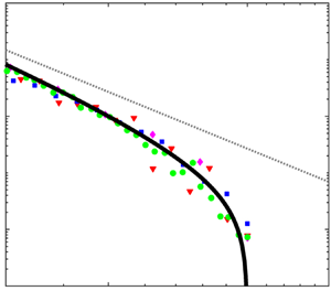
It has been previously noted (Deike et al. Reference Deike, Melville and Popinet2016) that bubble-size distributions deviate from a power law and become steeper for $a$ around $a_{max}$. Figure 3 shows bubble-size distributions from experiments and computational fluid dynamics simulations (scaled by $a_{max}$) of different entraining flows that exhibit such steepening. The distributions generally agree for $a \lesssim a_{max}$, but are not expected to be good for $a$ near $a_H$ (different values of $a_H/a_{max}$ for the data are listed in the figure caption). As large bubbles rise faster (Thorpe Reference Thorpe1982), the steepening for $a$ around $a_{max}$ has generally been attributed to degassing (Deike et al. Reference Deike, Melville and Popinet2016; Chan et al. Reference Chan, Johnson, Moin and Urzay2021). Garrett et al. (Reference Garrett, Li and Farmer2000) and Deike et al. (Reference Deike, Melville and Popinet2016) provided models for steepening due to degassing, also shown in figure 3.

Figure 3. Comparison of $N_{eq}$ prediction from (3.8) ($\gamma =-10/3$) (——-) with existing theories: - - -, equation (3.7) of Deike et al. (Reference Deike, Melville and Popinet2016); $\cdot\ \cdot\ \cdot\ \cdot\ \cdot\ \cdot$, $\propto a^{-16/3}$ (Garrett et al. Reference Garrett, Li and Farmer2000). Experiments: (i) $\square$ (blue), figure 5 of Deane et al. (Reference Deane, Stokes and Callaghan2016), case A. Simulations: (ii) $\triangledown$ (red), figure 7(e) of Deike et al. (Reference Deike, Melville and Popinet2016); (iii) $\diamond$ (magenta), figure 8 of Hendrickson et al. (Reference Hendrickson, Yu and Yue2020), ${\textit {Fr}}=0.192$; (iv) $\circ$ (green), figure 4d of Chan et al. (Reference Chan, Johnson, Moin and Urzay2021). Values for $a_H/a_{max}$ are approximately $0.35$, $0.15$, $0$, $0.15$ respectively for (i), (ii), (iii), (iv).

Because of the fast convergence discussed in § 4, we expect to observe $\tilde {\beta }_{eq}(a)$ given by (3.8) during active entrainment. In figure 3, we include $\tilde {\beta }_{eq}(a)$ using $\gamma =-10/3$ (Yu et al. Reference Yu, Hendrickson and Yue2020). Note that the shape does not change significantly with moderate variation of $\gamma$. From figure 3, we see that (3.8) exhibits the steepening of the bubble-size distribution for $a\sim a_{max}$, somewhat corroborated by existing measurements and simulations. Since (3.8) accounts only for fragmentation and cutoff power-law entrainment, this reveals a new mechanism for steepening deviation from a power law independent of other mechanisms such as degassing. The relative importance of these different mechanisms is a subject of current research.