


1. Introduction
Fluid flow through a curved pipe is encountered in various applications, from engineering equipment to biological systems. It is well-known that unidirectional laminar flow is not achievable in this system, as the balance between centrifugal force and pressure is disrupted, resulting in the formation of steady cross-stream vortices named after Dean’s seminal works (Dean Reference Dean1927, Reference Dean1928). The earliest qualitative observations of this flow pattern can be traced back to Boussinesq (Reference Boussinesq1868). Over the past century, Dean vortices have remained a fundamental example of secondary flows in fluid dynamics.
Extensive research into curved pipes has been conducted through experiments (White Reference White1929; Ito Reference Ito1959; Sreenivasan & Strykowski Reference Sreenivasan and Strykowski1983; Kuhnen et al. Reference Kühnen, Holzner, Hof and Kuhlmann2014,Reference Kühnen, Braunshier, Schwegel, Kuhlmann and Hof2015), theory (Dean Reference Dean1927; Van Dyke Reference Van Dyke1978; Daskopoulos & Lenhoff Reference Daskopoulos and Lenhoff1989; Boshier & Mestel Reference Boshier and Mestel2014, Reference Boshier and Mestel2017; Boshier & Mestel Reference Boshier and Mestel2014), and numerical computations (Collins & Dennis Reference Collins and Dennis1975; Patankar et al. Reference Patankar, Pratap and Spalding1975; Webster & Humphrey Reference Webster and Humphrey1997; Huttl & Friedrich Reference Hüttl and Friedrich2001; Piazza & Ciofalo Reference Piazza and Ciofalo2011). Readers seeking quick access to this vast body of work are encouraged to consult review articles by Berger et al. (Reference Berger, Talbot and Yao1983), Vashisth et al. (Reference Vashisth, Kumar and Nigam2008) and Vester et al. (Reference Vester, Örlü and Alfredsson2016). Numerical computations of curved pipe flows can be broadly categorised into those that use the so-called loose-coiling approximation, originating from Dean’s work, and those that do not, and this study belongs to the former category. The full curved pipe flow problem involves two parameters: the Reynolds number and the (dimensionless) curvature of the pipe. The loose-coiling approximation is valid when the curvature is small and the Reynolds number is large, allowing the behaviour of Dean vortices to be captured by a single parameter known as the Dean number. Historically, this approximation was particularly valuable when computational resources were limited. When the Dean number is small, perturbation theory can be applied, providing a useful check on numerical computations for finite Dean numbers.
In the 1980s and 1990s, significant interest centred on the non-uniqueness of steady vortex structures in the loose-coiling approximation system. Two families of four-vortex solutions were discovered numerically (Benjamin Reference Benjamin1978; Nandakumar & Masliyah Reference Nandakumar and Masliyah1982; Winters Reference Winters1987; Yanase et al. Reference Yanase, Goto and Yamamoto1989; Daskopoulos & Lenhoff Reference Daskopoulos and Lenhoff1989), and are later elegantly reconstructed via perturbation expansion (Boshier & Mestel Reference Boshier and Mestel2014, Reference Boshier and Mestel2017). These flow states can be regarded as what are now called exact coherent structures. Identifying exact coherent structures has become one of the major focuses in shear flow research, guided by dynamical systems theory (see e.g. Kerswell Reference Kerswell2005; Eckhardt et al. Reference Eckhardt, Schneider, Hof and Westerweel2007). However, previous studies on Dean vortices have only addressed two-dimensional stationary structures that are invariant along the pipe’s axial direction. The primary goal of this research is therefore to extend these theoretical and numerical results to three-dimensional travelling-wave-type exact coherent structures, providing a broader theoretical understanding of the complex dynamics in curved pipe flows.
Although stable travelling wave states have been observed under specific parameters in experiments and numerical simulations (Webster & Humphrey Reference Webster and Humphrey1993, Reference Webster and Humphrey1997), to the best of the authors’ knowledge, systematic continuation study of corresponding exact coherent structures by Newton’s method has not been conducted yet. Stability analysis of the Dean vortex with respect to three-dimensional perturbations serves as an obvious first step towards obtaining nonlinear travelling waves by bifurcation analysis. However, somewhat surprisingly, such stability analysis was not pursued until the recent work by Canton et al. (Reference Canton, Schlatter and Örlü2016).
Another pathway to finding a three-dimensional travelling wave is through homotopy continuation from the exact coherent structures obtained in a straight pipe flow (Faisst & Eckhardt Reference Faisst and Eckhardt2003; Wedin & Kerswell Reference Wedin and Kerswell2004; Pringle & Kerswell Reference Pringle and Kerswell2007; Pringle et al. Reference Pringle, Duguet and Kerswell2009). In the absence of curvature, no linear instability arises in the laminar Hagen–Poiseuille flow, thus the transition to turbulence is necessarily triggered by finite-amplitude perturbations. Exact coherent structures are crucial for an understanding of such subcritical transition problems (Kerswell Reference Kerswell2005; Eckhardt et al. Reference Eckhardt, Schneider, Hof and Westerweel2007). The physical mechanism by which coherent structures are maintained, independent of laminar flow instabilities, is commonly explained by a cyclic interaction between the rolls, streaks and waves (self-sustaining process; see Hamilton et al. Reference Hamilton, Kim and Waleffe1995; Waleffe Reference Waleffe1997). The cycle naturally emerges from the large-Reynolds-number asymptotic expansion of exact coherent structures in the high-Reynolds-number limit, known as the vortex–wave interaction (VWI) theory (see Hall & Smith Reference Hall and Smith1991; Hall & Sherwin Reference Hall and Sherwin2010; Deguchi & Hall Reference Deguchi and Hall2014, Ozcakir et al. Reference Ozcakir, Tanveer, Hall and Overman2016).
At medium to high curvatures of the pipe, Sreenivasan & Strykowski (Reference Sreenivasan and Strykowski1983), Webster & Humphrey (Reference Webster and Humphrey1993, Reference Webster and Humphrey1997) and Kuhnen et al. (Reference Kühnen, Holzner, Hof and Kuhlmann2014) identified a supercritical transition characterised by the emergence of a travelling wave. However, when the pipe curvature is small, the neutral curve recedes to higher Reynolds numbers, making subcritical transition, as observed in straight pipe flow problems, more dominant (Kuhnen et al. Reference Kühnen, Braunshier, Schwegel, Kuhlmann and Hof2015). Expanding on these findings, Canton et al. (Reference Canton, Rinaldi, Örlü and Schlatter2020) conducted detailed direct numerical simulations around the pipe curvature at which the nature of the transition changes from subcritical to supercritical. They observed that within a narrow range of pipe curvatures, the flow can exhibit both sustained turbulence and a stable travelling wave, with two competing attractors in the phase space. Moreover, the supercritical Hopf bifurcation point for the three-dimensional travelling waves detected by Canton et al. (Reference Canton, Rinaldi, Örlü and Schlatter2020) aligns perfectly with the neutral curve computed by the stability analysis (Canton et al. Reference Canton, Schlatter and Örlü2016).
One of the remaining unanswered questions is how the three-dimensional travelling waves that emerge in the supercritical transitions relate to the exact coherent structures self-sustained at the straight pipe case. This inquiry is closely tied to the works by Nagata (Reference Nagata1988, Reference Nagata1990), where exact coherent structures in plane Couette flow were found through continuation from secondary flows induced by system rotation. Another key question in this paper is the relationship between the Dean vortices in the loose-coiling approximation and the VWI theory, both of which apply in the high-Reynolds-number limit. Bridging these theories seems promising, given that the VWI originated from the asymptotic theory for Görtler vortices (Hall & Smith Reference Hall and Smith1988).
For plane Couette flow, Deguchi et al. (Reference Deguchi, Hall and Walton2013) showed that when the streamwise wavelength of exact coherent structures is comparable to the Reynolds number, the VWI approximation breaks down and must be replaced by boundary region equations (BRE). More recently, Dokoza & Oberlack (Reference Dokoza and Oberlack2023) considered the same limit to explain the large-scale coherent structures observed in direct numerical simulations in Lee & Moser (Reference Lee and Moser2019). We will show that two high-Reynolds-number limits, VWI and BRE, are also possible for the curved pipe flow problem.
The rest of the paper is organised as follows. In the next section, we will formulate the curved pipe flow problem using Navier–Stokes equations. The loose-coiling approximation and its extensions to the three-dimensional travelling waves will be discussed. Section 3 first studies the large Reynolds number asymptotic properties of the stability of the Dean vortices with respect to three-dimensional perturbations. In the same section, we will also study the bifurcation of nonlinear travelling waves. Section 4 is devoted to the continuation of exact coherent structures from the straight pipe problem. Finally, in § 5, we present our conclusions and discuss the implications of the results.
2. Formulation of the problem

Figure 1. A sketch of the curved pipe studied in this paper. The grey surface represents a section of a torus with minor and major radii denoted by
 $a^*$
and
$a^*$
and
 $d^*$
, respectively. The flow field is described by the orthogonal coordinates
$d^*$
, respectively. The flow field is described by the orthogonal coordinates
 $(r^*,\theta ,z^*)$
.
$(r^*,\theta ,z^*)$
.
Consider an incompressible Newtonian viscous fluid with density
 $\rho ^*$
and dynamic viscosity
$\rho ^*$
and dynamic viscosity
 $\mu ^*$
flowing through a curved circular pipe. As sketched in figure 1, we denote the radius of the curvature of the pipe centreline as
$\mu ^*$
flowing through a curved circular pipe. As sketched in figure 1, we denote the radius of the curvature of the pipe centreline as
 $d^*$
, and the radius of the pipe as
$d^*$
, and the radius of the pipe as
 $a^*$
, with the latter chosen as the length scale. Following Germano (Reference Germano1982, Reference Germano1989), the orthogonal coordinates
$a^*$
, with the latter chosen as the length scale. Following Germano (Reference Germano1982, Reference Germano1989), the orthogonal coordinates
 $(r^*,\theta ,z^*)$
are installed to describe the radial, circumferential and streamwise directions, respectively. We assume that the flow is driven by a constant pressure gradient
$(r^*,\theta ,z^*)$
are installed to describe the radial, circumferential and streamwise directions, respectively. We assume that the flow is driven by a constant pressure gradient
 $G^*$
. In the absence of the curvature, the centreline velocity of the laminar Hagen–Poiseuille flow is given by
$G^*$
. In the absence of the curvature, the centreline velocity of the laminar Hagen–Poiseuille flow is given by
 $U_c^*= ({G^* a^{*2}})/({4 \mu ^*})$
, and we adopt this as the velocity scale. The non-dimensional velocity field
$U_c^*= ({G^* a^{*2}})/({4 \mu ^*})$
, and we adopt this as the velocity scale. The non-dimensional velocity field
 $(u,v,w)$
and pressure
$(u,v,w)$
and pressure
 $p$
are governed by the Navier–Stokes equations
$p$
are governed by the Navier–Stokes equations
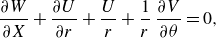
 \begin{eqnarray} \omega\, \frac {\partial w}{\partial z}+\frac {\partial u}{\partial r}+\frac {u}{r}+\frac {1}{r}\,\frac {\partial v}{\partial \theta }+\kappa \omega \{u\cos \theta -v\sin \theta \}=0,\end{eqnarray}
 \begin{eqnarray} \frac {{\rm D}u}{{\rm D}t}-\frac {v^2}{r}-\kappa \omega w^2\cos \theta =-\frac {\partial p}{\partial r}+\frac {1}{R} \left \{\left (\frac {1}{r}\,\frac {\partial }{\partial \theta }-\kappa \omega \sin \theta \right )S_1-\omega\, \frac {\partial S_3}{\partial z} \right \}, \end{eqnarray}
 \begin{eqnarray} \frac {{\rm D}v}{{\rm D}t}+\frac {uv}{r}+\kappa \omega w^2 \sin \theta =-\frac {1}{r}\,\frac {\partial p}{\partial \theta }+\frac {1}{R}\left \{\omega\, \frac {\partial S_2}{\partial z}-\left (\frac {\partial }{\partial r}+\kappa \omega \cos \theta \right )S_1\right \}, \end{eqnarray}
 \begin{eqnarray} \frac {{\rm D}w}{{\rm D}t}+ \kappa \omega w(u\cos \theta -v\sin \theta )=-\omega\, \frac {\partial p}{\partial z}+\frac {1}{R} \left \{4+\left (\frac {1}{r}+\frac {\partial }{\partial r}\right )S_3-\frac {1}{r}\,\frac {\partial S_2}{\partial \theta }\right \},\end{eqnarray}
where
 $r=r^*/a^*$
,
$r=r^*/a^*$
,
 $z=z^*/a^*$
and
$z=z^*/a^*$
and
 \begin{eqnarray} \frac {{\rm D}}{{\rm D}t}=\frac {\partial }{\partial t}+\omega w\, \frac {\partial }{\partial z}+u\,\frac {\partial }{\partial r}+\frac {v}{r}\,\frac {\partial }{\partial \theta },\quad \omega =\frac {1}{1+\kappa r \cos \theta }, \end{eqnarray}
 \begin{eqnarray} S_1=\frac {1}{r}\,\frac {\partial u}{\partial \theta }-\frac {\partial v}{\partial r}-\frac {v}{r},\quad S_2=\omega\, \frac {\partial v}{\partial z}+\kappa \omega w \sin \theta -\frac {1}{r}\,\frac {\partial w}{\partial \theta }, \end{eqnarray}
 \begin{eqnarray} S_3=\frac {\partial w}{\partial r}+\kappa \omega w\cos \theta -\omega\, \frac {\partial u}{\partial z}.\end{eqnarray}
The flow has two parameters, the Reynolds number and the non-dimensional curvature:
 \begin{equation} R=\frac {U_c^* a^*\rho ^*}{\mu ^*}, \quad \kappa = \frac {a^*}{d^*}. \end{equation}
The no-slip conditions
 $u=v=w=0$
are imposed at
$u=v=w=0$
are imposed at
 $r=1$
. In the streamwise direction, the flow is assumed to be periodic with period
$r=1$
. In the streamwise direction, the flow is assumed to be periodic with period
 ${2\pi }/{\alpha }$
, where
${2\pi }/{\alpha }$
, where
 $\alpha$
is the wavenumber. Our Reynolds number
$\alpha$
is the wavenumber. Our Reynolds number
 $R$
is based on the pressure gradient; therefore, the bulk velocity
$R$
is based on the pressure gradient; therefore, the bulk velocity
 $Q$
(i.e. normalised flux) is one of the appropriate quantities to diagnose the flow state.
$Q$
(i.e. normalised flux) is one of the appropriate quantities to diagnose the flow state.
As Dean (Reference Dean1927) realised, the combined parameter
 $K\equiv 2\kappa R^2$
plays an important role when the curvature
$K\equiv 2\kappa R^2$
plays an important role when the curvature
 $\kappa$
is small (see § 2.1). This is one of the widely used definitions of the ‘Dean number’ found in the literature. In experiments, however, the flux is easier to control, and
$\kappa$
is small (see § 2.1). This is one of the widely used definitions of the ‘Dean number’ found in the literature. In experiments, however, the flux is easier to control, and
 $De\equiv RQ\kappa ^{1/2}=Q(K/2)^{1/2}$
is more commonly used (see Vester et al. Reference Vester, Örlü and Alfredsson2016). Since
$De\equiv RQ\kappa ^{1/2}=Q(K/2)^{1/2}$
is more commonly used (see Vester et al. Reference Vester, Örlü and Alfredsson2016). Since
 $Q$
depends on
$Q$
depends on
 $R$
in a non-trivial manner, numerical computations are necessary to link
$R$
in a non-trivial manner, numerical computations are necessary to link
 $K$
with
$K$
with
 $De$
.
$De$
.
If the curvature
 $\kappa$
is not small, then the flow cannot be controlled by the Dean number alone (see e.g. Topakoglu Reference Topakoglu1967), and our study does not cover such a parameter regime.
$\kappa$
is not small, then the flow cannot be controlled by the Dean number alone (see e.g. Topakoglu Reference Topakoglu1967), and our study does not cover such a parameter regime.
2.1. Dean vortices
Suppose that the flow is steady and does not depend on
 $z$
. The loose-coiling approximation corresponds to the asymptotic limit of
$z$
. The loose-coiling approximation corresponds to the asymptotic limit of
 $R \to \infty$
,
$R \to \infty$
,
 $\kappa \to 0$
while keeping the Dean number
$\kappa \to 0$
while keeping the Dean number
 $K=2\kappa R^2$
as an
$K=2\kappa R^2$
as an
 $O(1)$
quantity. Substituting the asymptotic expansions
$O(1)$
quantity. Substituting the asymptotic expansions
 \begin{eqnarray} u=R^{-1}\,U(r,\theta )+\cdots ,\quad v=R^{-1}\,V(r,\theta )+\cdots , \end{eqnarray}
 \begin{eqnarray} w=W(r,\theta )+\cdots , \quad p=R^{-2}\,P(r,\theta )+\cdots ,\end{eqnarray}
into (2.1), and retaining the leading-order terms, we obtain the set of equations
 \begin{eqnarray} \frac {\partial U}{\partial r}+\frac {U}{r}+\frac {1}{r}\,\frac {\partial V}{\partial \theta }=0, \end{eqnarray}
 \begin{eqnarray} U\,\frac {\partial U}{\partial r}+\frac {V}{r}\,\frac {\partial U}{\partial \theta }-\frac {V^2}{r}-\frac {K}{2}\, W^2\cos \theta =-\frac {\partial P}{\partial r}+ \Delta _2 U-\frac {U}{r^2}-\frac {2}{r^2}\,\frac {\partial V}{\partial \theta } , \end{eqnarray}
 \begin{eqnarray} U\,\frac {\partial V }{\partial r}+\frac {V}{r}\,\frac {\partial V}{\partial \theta }+\frac {UV}{r}+\frac {K}{2}\, W^2 \sin \theta =-\frac {1}{r}\,\frac {\partial P}{\partial \theta }+ \Delta_2 V-\frac {V}{r^2}+\frac {2}{r^2}\,\frac {\partial U}{\partial \theta } ,\,\,\,\,\, \end{eqnarray}
 \begin{eqnarray} U\,\frac {\partial W}{\partial r}+\frac {V}{r}\,\frac {\partial W}{\partial \theta }=4+ \Delta_2 W. \end{eqnarray}
Here,
 \begin{eqnarray} \Delta_2=\partial _r^2+r^{-1}\,\partial _r+r^{-2}\,\partial _{\theta }^2 \end{eqnarray}
is the two-dimensional Laplacian operator. The no-slip conditions
 $U=V=W=0$
must be fulfilled at
$U=V=W=0$
must be fulfilled at
 $r=1$
. Equations (2.4) are equivalent to (15)–(18) of Dean (Reference Dean1928).
$r=1$
. Equations (2.4) are equivalent to (15)–(18) of Dean (Reference Dean1928).

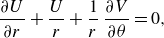
Figure 2. (a) Dependence on
 $K$
of the total average velocity
$K$
of the total average velocity
 $Q$
. The dashed green curve is the approximation (2.6), neglecting the
$Q$
. The dashed green curve is the approximation (2.6), neglecting the
 $O(K^6)$
terms. (b) The same 4-vortex solutions as in (a), but expressed in terms of the deviation of
$O(K^6)$
terms. (b) The same 4-vortex solutions as in (a), but expressed in terms of the deviation of
 $Q$
from the 2-vortex solution. The values of
$Q$
from the 2-vortex solution. The values of
 $K$
at the saddle–node bifurcation points are
$K$
at the saddle–node bifurcation points are
 $K_1\approx 5.71 \times 10^4$
,
$K_1\approx 5.71 \times 10^4$
,
 $K_2 \approx 3.89\times 10^5$
.
$K_2 \approx 3.89\times 10^5$
.
When
 $K=0$
, a unidirectional laminar flow solution
$K=0$
, a unidirectional laminar flow solution
 $(U,V,W)=(0,0,1-r^2)$
exists. As the curvature increases, a pair of streamwise vortices develops; hereafter, this state is referred to as the 2-vortex solution. Dean (Reference Dean1928) found this solution using a perturbation approach, and obtained the following approximation for the bulk velocity
$(U,V,W)=(0,0,1-r^2)$
exists. As the curvature increases, a pair of streamwise vortices develops; hereafter, this state is referred to as the 2-vortex solution. Dean (Reference Dean1928) found this solution using a perturbation approach, and obtained the following approximation for the bulk velocity
 $Q= ({1}/{\pi }) (\int ^{2\pi }_0\int ^1_0 W (r,\theta )\, {\rm d}r\, {\rm d}\theta)$
:
$Q= ({1}/{\pi }) (\int ^{2\pi }_0\int ^1_0 W (r,\theta )\, {\rm d}r\, {\rm d}\theta)$
:
 \begin{eqnarray} Q_2 \approx \frac {1}{2}\left (1-0.0306\left (\frac {K}{576} \right )^2+0.0120\left (\frac {K}{576} \right )^4+O(K^6) \right ). \end{eqnarray}
Here, the subscript 2 indicates that this result is valid for the 2-vortex solution, and
 $K=576$
corresponds to
$K=576$
corresponds to
 $De\approx 16.59$
. Attempts to extend the radius of convergence of the perturbation expansion were made by Van Dyke (Reference Van Dyke1978), and more recently Boshier & Mestel (Reference Boshier and Mestel2014, Reference Boshier and Mestel2017) successfully reproduced the two families of 4-vortex solutions previously reported numerically (Benjamin Reference Benjamin1978; Winters Reference Winters1987; Yanase et al. Reference Yanase, Goto and Yamamoto1989; Daskopoulos & Lenhoff Reference Daskopoulos and Lenhoff1989). Figure 2(a) summarises the variation of
$De\approx 16.59$
. Attempts to extend the radius of convergence of the perturbation expansion were made by Van Dyke (Reference Van Dyke1978), and more recently Boshier & Mestel (Reference Boshier and Mestel2014, Reference Boshier and Mestel2017) successfully reproduced the two families of 4-vortex solutions previously reported numerically (Benjamin Reference Benjamin1978; Winters Reference Winters1987; Yanase et al. Reference Yanase, Goto and Yamamoto1989; Daskopoulos & Lenhoff Reference Daskopoulos and Lenhoff1989). Figure 2(a) summarises the variation of
 $Q$
for 2- and 4-vortex solutions. To gain a clearer understanding of the bifurcations, it is helpful to summarise the results in terms of the deviation from the 2-vortex value,
$Q$
for 2- and 4-vortex solutions. To gain a clearer understanding of the bifurcations, it is helpful to summarise the results in terms of the deviation from the 2-vortex value,
 $\Delta Q\equiv Q-Q_2$
(Figure 2
b). The 2-vortex solution is known to be stable for
$\Delta Q\equiv Q-Q_2$
(Figure 2
b). The 2-vortex solution is known to be stable for
 $z$
-independent perturbations in the range of
$z$
-independent perturbations in the range of
 $K$
shown in the figure. However, it becomes unstable against more general perturbations at a critical
$K$
shown in the figure. However, it becomes unstable against more general perturbations at a critical
 $K$
, as we will see in § 3.
$K$
, as we will see in § 3.
2.2. Numerical methods
Our aim is to extend the above argument to three-dimensional travelling waves. An examination reveals that except for the terms involving
 $K$
, (2.4) matches the Navier–Stokes equations in cylindrical coordinates, but with a unit Reynolds number and no
$K$
, (2.4) matches the Navier–Stokes equations in cylindrical coordinates, but with a unit Reynolds number and no
 $z$
-dependence. Therefore, a naive approach would be to simplify the full governing equations (2.1) to
$z$
-dependence. Therefore, a naive approach would be to simplify the full governing equations (2.1) to
 \begin{eqnarray} \frac {\partial w}{\partial z}+\frac {\partial u}{\partial r}+\frac {u}{r}+\frac {1}{r}\,\frac {\partial v}{\partial \theta }=0, \end{eqnarray}
 \begin{eqnarray} \frac {{\rm D}u}{{\rm D}t}-r^{-1}v^2- \frac {K}{2} \left (\frac {w}{R} \right )^2 \cos \theta = -\frac {\partial p}{\partial r}+ \frac {1}{R}\left(\Delta u-r^{-2}u-2r^{-2}\,\frac {\partial v}{\partial \theta }\right),\,\,\, \end{eqnarray}
 \begin{eqnarray} \frac {{\rm D}v}{{\rm D}t}+r^{-1}uv+ \frac {K}{2} \left (\frac {w}{R} \right )^2 \sin \theta =-r^{-1}\,\frac {\partial p}{\partial \theta }+\frac {1}{R}\left(\Delta v -r^{-2}v+2r^{-2}\frac {\partial u}{\partial \theta }\right), \end{eqnarray}
 \begin{eqnarray} \frac {{\rm D}w}{{\rm D}t}=-\frac {\partial p}{\partial z}+\frac {1}{R}\,(4+\Delta w), \end{eqnarray}
where
 $ {{\rm D}}/{{\rm D}t}=\partial _t+u\,\partial _r+r^{-1}v\,\partial _{\theta }+w\,\partial _z$
and
$ {{\rm D}}/{{\rm D}t}=\partial _t+u\,\partial _r+r^{-1}v\,\partial _{\theta }+w\,\partial _z$
and
 $\unicode{x1D6E5} =\partial _r^2+r^{-1}\,\partial _r+r^{-2}\,\partial _{\theta }^2+\partial _z^2$
. It is easy to verify that (i) when
$\unicode{x1D6E5} =\partial _r^2+r^{-1}\,\partial _r+r^{-2}\,\partial _{\theta }^2+\partial _z^2$
. It is easy to verify that (i) when
 $K=0$
, (2.7) become the three-dimensional Navier–Stokes equations governing the straight pipe flow problem, and (ii) the leading-order parts of the Dean vortex solutions satisfy (2.7).
$K=0$
, (2.7) become the three-dimensional Navier–Stokes equations governing the straight pipe flow problem, and (ii) the leading-order parts of the Dean vortex solutions satisfy (2.7).
The use of the above equations can be justified by asymptotic analysis. To clarify the discussion, we will define a terminology: we will refer to a reduced system as asymptotic preserving reduction (APR) when it contains all the essential components to yield the leading-order solution of the full equations (2.1). We will demonstrate that in the same limit considered by Dean (Reference Dean1927), there are two possible sets of reduced equations for three-dimensional coherent structures, and that (2.7) is APR of both of them.
All numerical results in this paper are based on (2.7), including figure 2. In order to find nonlinear travelling wave solutions
 $\mathbf {u}(r,\theta ,z-ct)$
, we apply a Galilean shift to eliminate the time dependence. Our numerical code is based on Deguchi & Nagata (Reference Deguchi and Nagata2011), where the poloidal–toroidal decomposition
$\mathbf {u}(r,\theta ,z-ct)$
, we apply a Galilean shift to eliminate the time dependence. Our numerical code is based on Deguchi & Nagata (Reference Deguchi and Nagata2011), where the poloidal–toroidal decomposition
 $\mathbf {u}= \mathcal {W}(r)\,\mathbf {e}_z+\nabla \times \nabla \times (\phi (r,\theta ,z)\, \mathbf {e}_r)+\nabla \times (\psi (r,\theta ,z)\, \mathbf {e}_r)$
is used. The continuity is automatically satisfied, and the independent equations can be obtained by operating
$\mathbf {u}= \mathcal {W}(r)\,\mathbf {e}_z+\nabla \times \nabla \times (\phi (r,\theta ,z)\, \mathbf {e}_r)+\nabla \times (\psi (r,\theta ,z)\, \mathbf {e}_r)$
is used. The continuity is automatically satisfied, and the independent equations can be obtained by operating
 $\mathbf {e}_r\cdot \nabla \times \nabla \times{}$
,
$\mathbf {e}_r\cdot \nabla \times \nabla \times{}$
,
 $\mathbf {e}_r\cdot \nabla \times{}$
and the
$\mathbf {e}_r\cdot \nabla \times{}$
and the
 $\theta$
-
$\theta$
-
 $z$
average to the momentum equations. The basis functions for the poloidal potential
$z$
average to the momentum equations. The basis functions for the poloidal potential
 $\phi$
, toroidal potential
$\phi$
, toroidal potential
 $\psi$
, and mean flow
$\psi$
, and mean flow
 $\mathcal {W}$
are the same as those used in Deguchi & Walton (Reference Deguchi and Walton2013). A Fourier–Galerkin method is used in the
$\mathcal {W}$
are the same as those used in Deguchi & Walton (Reference Deguchi and Walton2013). A Fourier–Galerkin method is used in the
 $\theta$
and
$\theta$
and
 $z$
directions, while a Chebyshev collocation method is employed in the
$z$
directions, while a Chebyshev collocation method is employed in the
 $r$
direction. This transforms the problem into a set of algebraic equations, with the spectral coefficients and phase speed
$r$
direction. This transforms the problem into a set of algebraic equations, with the spectral coefficients and phase speed
 $c$
as unknowns, which can then be solved using Newton’s method. The truncation level of the expansions is specified using the triplet
$c$
as unknowns, which can then be solved using Newton’s method. The truncation level of the expansions is specified using the triplet
 $(L,M,N)$
, where
$(L,M,N)$
, where
 $L$
is the degree of Chebyshev polynomials, and
$L$
is the degree of Chebyshev polynomials, and
 $M$
and
$M$
and
 $N$
are the orders of Fourier series in the
$N$
are the orders of Fourier series in the
 $\theta$
and
$\theta$
and
 $z$
directions, respectively.
$z$
directions, respectively.
Since we have the Jacobian matrix at hand, stability analysis can be performed readily. The complete list of eigenvalues is first computed by the LAPACK routine ZGGEV. The most unstable mode is then tracked in the parameter space using the well-known Rayleigh quotient iteration scheme (Lloyd & David Reference Lloyd and David1997). If good initial guesses are provided, then this method allows accurate eigenvalues and eigenvectors to be obtained with just a handful of numerically low-cost iterations.
3. Bifurcation from the 2-vortex solution
3.1. Linear stability of the 2-vortex solution
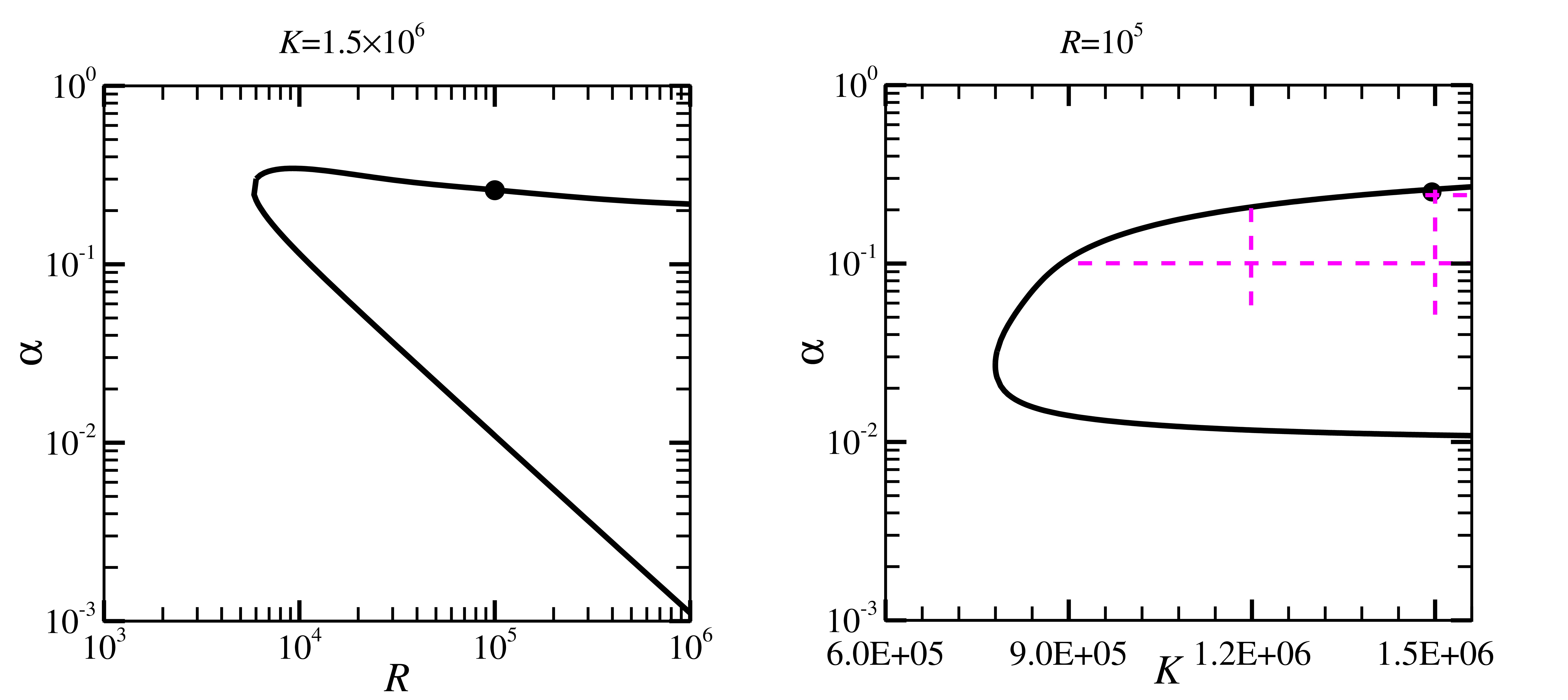
Figure 3. The stability of the 2-vortex solution found by the Orr–Sommerfeld equations (3.2). (a) The neutral curve in the
 $ \alpha$
–
$ \alpha$
–
 $R$
plane at
$R$
plane at
 $K=1.5 \times 10^6$
. The upper curve is the inviscid mode. (b) The neutral curve in the
$K=1.5 \times 10^6$
. The upper curve is the inviscid mode. (b) The neutral curve in the
 $\alpha$
–
$\alpha$
–
 $K$
plane at
$K$
plane at
 $R=10^{5}$
. The dots represent the same point in the parameter space. The magenta dashed lines indicate the parameter range studied in figure 5. The spatial resolution is checked using up to
$R=10^{5}$
. The dots represent the same point in the parameter space. The magenta dashed lines indicate the parameter range studied in figure 5. The spatial resolution is checked using up to
 $(L,M)=(50,50)$
.
$(L,M)=(50,50)$
.
The linear stability of the Dean vortices can be analysed by introducing a perturbation
 $\mathbf {u}=(R^{-1}U,R^{-1}V,W)+ (\tilde u, \tilde v, \tilde w)$
,
$\mathbf {u}=(R^{-1}U,R^{-1}V,W)+ (\tilde u, \tilde v, \tilde w)$
,
 $p=R^{-2}P+\tilde {p}$
. The perturbation is assumed to be proportional to an infinitesimally small amplitude
$p=R^{-2}P+\tilde {p}$
. The perturbation is assumed to be proportional to an infinitesimally small amplitude
 $\delta \gt 0$
and a normal mode as
$\delta \gt 0$
and a normal mode as
 \begin{eqnarray} (\tilde u, \tilde v, \tilde w, \tilde p)=\delta (\hat {u}(r,\theta ),\hat {v}(r,\theta ),\hat {w}(r,\theta ),\hat {p}(r,\theta ))\,{\rm e}^{{\textrm i}\alpha z+\sigma t}+\text {c.c.}, \end{eqnarray}
where c.c. stands for the complex conjugate. The real part of the complex growth rate
 $\sigma = \sigma _r + {\textrm i} \sigma _i$
determines the stability.
$\sigma = \sigma _r + {\textrm i} \sigma _i$
determines the stability.
Given that Dean’s limit corresponds to the high Reynolds number regime, the base flow may be dominated by
 $W$
. Moreover, the advection effect by that component is much stronger than the curvature effects of
$W$
. Moreover, the advection effect by that component is much stronger than the curvature effects of
 $O(R^{-2})$
(see (2.7)). If we are allowed to neglect
$O(R^{-2})$
(see (2.7)). If we are allowed to neglect
 $U$
,
$U$
,
 $V$
and the terms proportional to
$V$
and the terms proportional to
 $K$
, then the stability can be found by the Orr–Sommerfeld equation generalised for the base flow varying in two directions:
$K$
, then the stability can be found by the Orr–Sommerfeld equation generalised for the base flow varying in two directions:
 \begin{eqnarray} \frac {\partial \hat {u}}{\partial r}+\frac {\hat {u}}{r}+\frac {1}{r}\,\frac {\partial \hat {v}}{\partial \theta }+ {\textrm i} \alpha \hat { w}=0, \end{eqnarray}
 \begin{eqnarray} (\sigma +{\textrm {i}}\alpha W) \hat {u}=-\frac {\partial \hat {p}}{\partial r}+\frac {1}{R}\left \{(\Delta_2 -\alpha ^2) \hat {u} -\frac {\hat {u}}{r^2}-\frac {2}{r^2}\,\frac {\partial \hat {v}}{\partial \theta }\right \}, \end{eqnarray}
 \begin{eqnarray} (\sigma + {\textrm {i}}\alpha W) \hat {v}=-\frac {1}{r}\,\frac {\partial \hat {p}}{\partial \theta }+\frac {1}{R}\left \{(\Delta _2 -\alpha ^2) \hat {v}-\frac {\hat {v}}{r^2}+\frac {2}{r^2}\,\frac {\partial \hat {u}}{\partial \theta }\right \}, \end{eqnarray}
 \begin{eqnarray} (\sigma +{\textrm {i}}\alpha W) \hat {w}+\hat {u}\,\frac {\partial W}{\partial r}+\frac {\hat {v}}{r}\,\frac {\partial W}{\partial \theta }=- {\textrm i} \alpha { \hat {p}}+\frac {1}{R}\,(\Delta_2 -\alpha ^2) \hat {w}. \end{eqnarray}
Here,
 $\Delta_2$
is the operator defined in (2.5). The no-slip conditions
$\Delta_2$
is the operator defined in (2.5). The no-slip conditions
 $\hat {u}=\hat {v}=\hat {w}=0$
are imposed at
$\hat {u}=\hat {v}=\hat {w}=0$
are imposed at
 $r=1$
. Using the 2-vortex solution as the base state at
$r=1$
. Using the 2-vortex solution as the base state at
 $K=1.5\times 10^6$
, the eigenvalue problem yields the neutral curve shown in figure 3(a). The upper neutral curve tends to a constant value of
$K=1.5\times 10^6$
, the eigenvalue problem yields the neutral curve shown in figure 3(a). The upper neutral curve tends to a constant value of
 $\alpha$
as
$\alpha$
as
 $R$
increases, which is a typical feature of inviscid instability. Note that for neutral modes, the viscous terms are still important around the critical layer, where
$R$
increases, which is a typical feature of inviscid instability. Note that for neutral modes, the viscous terms are still important around the critical layer, where
 $W-c$
vanishes. Nevertheless, for sufficiently large
$W-c$
vanishes. Nevertheless, for sufficiently large
 $R$
, the generalised Orr–Sommerfeld result matches with the inviscid result (Deguchi Reference Deguchi2019). Since computations become challenging at very high Reynolds numbers, this paper will use
$R$
, the generalised Orr–Sommerfeld result matches with the inviscid result (Deguchi Reference Deguchi2019). Since computations become challenging at very high Reynolds numbers, this paper will use
 $R=10^5$
to infer results involving inviscid waves. Figure 3(b) shows the neutral curve obtained by varying
$R=10^5$
to infer results involving inviscid waves. Figure 3(b) shows the neutral curve obtained by varying
 $K$
at that fixed
$K$
at that fixed
 $R$
. The instability exists only for
$R$
. The instability exists only for
 $K \gtrsim 7.78\times 10^5$
(
$K \gtrsim 7.78\times 10^5$
(
 $De\gtrsim\, 289.69$
). The inviscid mode serves as a starting point of the analysis of the VWI-type nonlinear solutions in § 3.2.
$De\gtrsim\, 289.69$
). The inviscid mode serves as a starting point of the analysis of the VWI-type nonlinear solutions in § 3.2.
One might worry about the validity of neglecting the curvature terms in (3.2) given the large values of
 $K$
. The size of the curvature term in the linearised version of (2.7) is
$K$
. The size of the curvature term in the linearised version of (2.7) is
 $K/R^2$
multiplied by the wave amplitude, whereas the viscous term scales as
$K/R^2$
multiplied by the wave amplitude, whereas the viscous term scales as
 $O(1/R)$
times the wave amplitude. The size of the latter term increases by
$O(1/R)$
times the wave amplitude. The size of the latter term increases by
 $O(R^{2/3})$
within the critical layer of thickness
$O(R^{2/3})$
within the critical layer of thickness
 $O(R^{-1/3})$
. Hence the condition for safely neglecting the curvature term is
$O(R^{-1/3})$
. Hence the condition for safely neglecting the curvature term is
 $KR^{-2} \ll O(R^{-1/3})$
. For
$KR^{-2} \ll O(R^{-1/3})$
. For
 $K=10^6$
, this condition is satisfied as long as
$K=10^6$
, this condition is satisfied as long as
 $R\gg 4000$
, which is not difficult to achieve in pipe flows.
$R\gg 4000$
, which is not difficult to achieve in pipe flows.

Figure 4. The stability results based on the linearised version of (2.7) around the 2-vortex solution. (a) The neutral curve of the curvature mode in the
 $\alpha _0$
–
$\alpha _0$
–
 $R$
plane at
$R$
plane at
 $K=60\,600$
. The long-wavelength limit (3.4) is achieved as
$K=60\,600$
. The long-wavelength limit (3.4) is achieved as
 $R\rightarrow \infty .$
(b) The neutral curve in the
$R\rightarrow \infty .$
(b) The neutral curve in the
 $ \alpha _0$
–
$ \alpha _0$
–
 $K$
plane at
$K$
plane at
 $R=10^{6}$
. The bullets represent the same point in the parameter space. The magenta dashed lines indicate the parameter range studied in figure 7. Resolution is checked using up to
$R=10^{6}$
. The bullets represent the same point in the parameter space. The magenta dashed lines indicate the parameter range studied in figure 7. Resolution is checked using up to
 $(L,M)=(50,50)$
.
$(L,M)=(50,50)$
.
Along the lower neutral curve in figure 3(a), the wavenumber
 $\alpha$
behaves like
$\alpha$
behaves like
 $O(R^{-1})$
, which is a typical signature of the emergence of the long-wavelength mode. This observation motivates us to take the limit
$O(R^{-1})$
, which is a typical signature of the emergence of the long-wavelength mode. This observation motivates us to take the limit
 $R\rightarrow \infty$
while keeping
$R\rightarrow \infty$
while keeping
 $\alpha _0\equiv R\alpha$
as a constant, similar to the method used for unidirectional parallel flows (Smith Reference Smith1979; Cowley & Smith Reference Cowley and Smith1985). However, in this limit, the advection effect due to
$\alpha _0\equiv R\alpha$
as a constant, similar to the method used for unidirectional parallel flows (Smith Reference Smith1979; Cowley & Smith Reference Cowley and Smith1985). However, in this limit, the advection effect due to
 $W$
becomes
$W$
becomes
 $W\partial _z=O(R^{-1})$
, making the advection effects due to
$W\partial _z=O(R^{-1})$
, making the advection effects due to
 $U$
and
$U$
and
 $V$
non-negligible. Furthermore, from the continuity equation,
$V$
non-negligible. Furthermore, from the continuity equation,
 $\tilde {u}$
,
$\tilde {u}$
,
 $\tilde {v}$
are smaller than
$\tilde {v}$
are smaller than
 $\tilde {w}$
by a factor of
$\tilde {w}$
by a factor of
 $O(R^{-1})$
, similar to Dean’s argument, which necessitates retaining the curvature terms. Formally, the long-wavelength limit can be obtained by rescaling
$O(R^{-1})$
, similar to Dean’s argument, which necessitates retaining the curvature terms. Formally, the long-wavelength limit can be obtained by rescaling
 $\alpha =R^{-1}\alpha _0$
,
$\alpha =R^{-1}\alpha _0$
,
 $\sigma =R^{-1}{\sigma _0}$
and writing
$\sigma =R^{-1}{\sigma _0}$
and writing
 \begin{eqnarray} (\tilde u, \tilde v, \tilde w, \tilde p)=\delta R^{-1} (\hat {u}(r,\theta ),\hat {v}(r,\theta ),R\, \hat {w}(r,\theta ),R^{-1}\,\hat {p}(r,\theta ))\,{\rm e}^{R^{-1}({\textrm i}{\alpha _0} z+{\sigma _0} t)}+\text {c.c.},\,\,\,\, \end{eqnarray}
in (2.7). The leading-order problem can be found as
 \begin{align} & \frac {\partial \hat {u}}{\partial r}+\frac {\hat {u}}{r}+\frac {1}{r}\,\frac {\partial \widehat {v}}{\partial \theta }+ {\textrm i} \alpha _0 \hat { w}=0, \end{align}
 \begin{align} & \left( \mathcal {L} +\frac { \partial U }{\partial r} + \frac {1}{r^2} \right) \hat {u}+\left(\frac {1}{r}\,\frac {\partial U}{\partial \theta } - \frac {2V}{r} +\frac {2}{r^2}\,\frac { \partial }{ \partial \theta } \right) \hat {v} -K W \hat {w}\cos \theta +\frac { \partial \widehat { p}}{\partial r}=0, \end{align}
 \begin{align} & \left( \mathcal {L} +\frac {1}{r}\,\frac { \partial V }{ \partial \theta } + \frac {1}{r^2} +\frac {U}{r} \right) \hat {v}+\left(\frac {1}{r}\,\frac {\partial (r V)}{ \partial r} -\frac {2}{r^2}\,\frac { \partial }{ \partial \theta } \right) \hat {u} +K W \hat {w}\sin \theta +\frac {1}{r}\,\frac { \partial \widehat { p}}{ \partial \theta }=0, \end{align}
 \begin{align} &\mathcal {L} \hat {w}+\frac {\partial W}{\partial r}\, \hat { u} +\frac {1}{r}\,\frac {\partial W}{ \partial \theta }\, \hat {v}=0. \end{align}
Here, we have defined the operator
 $\mathcal {L} = ({\sigma _0} + {\textrm i} \alpha _0 W +U ({\partial }/{\partial r})+ ({V}/{r})({\partial }/{\partial \theta })-\Delta_2 )$
to simplify the equations. The usual no-slip conditions complete the eigenvalue problem.
$\mathcal {L} = ({\sigma _0} + {\textrm i} \alpha _0 W +U ({\partial }/{\partial r})+ ({V}/{r})({\partial }/{\partial \theta })-\Delta_2 )$
to simplify the equations. The usual no-slip conditions complete the eigenvalue problem.
Figure 4(a) shows the stability of the 2-vortex solution by using the linearised version of (2.7). Along both branches of the neutral curve, as
 $R\rightarrow \infty$
, the value of
$R\rightarrow \infty$
, the value of
 $\alpha _0$
tends to a constant, which corresponds to the limit shown in (3.4). Interestingly, this result suggests that our analysis detects a new mode, disconnected from the mode seen in figure 3(a). Hereafter, the new mode is referred to as the ‘curvature mode’ as its existence depends on the presence of the terms proportional to
$\alpha _0$
tends to a constant, which corresponds to the limit shown in (3.4). Interestingly, this result suggests that our analysis detects a new mode, disconnected from the mode seen in figure 3(a). Hereafter, the new mode is referred to as the ‘curvature mode’ as its existence depends on the presence of the terms proportional to
 $K$
. At the large
$K$
. At the large
 $R$
limit, the lower branch of the neutral curve shown in figure 3(a) may be governed by the same limiting equations; however, we do not examine it further in this paper.
$R$
limit, the lower branch of the neutral curve shown in figure 3(a) may be governed by the same limiting equations; however, we do not examine it further in this paper.
The solid curve in figure 4(b) shows the neutral curve obtained with
 $R=10^6$
, which is sufficiently large to observe the converged limiting solution. This figure clearly shows that the curvature mode exists only when
$R=10^6$
, which is sufficiently large to observe the converged limiting solution. This figure clearly shows that the curvature mode exists only when
 $K$
is larger than the critical value
$K$
is larger than the critical value
 $5.72\times 10^4$
. In terms of the flux-based parameter, this critical point corresponds to
$5.72\times 10^4$
. In terms of the flux-based parameter, this critical point corresponds to
 $De\approx 110$
. It is noteworthy that recently Lupi et al. (Reference Lupi, Canton, Rinaldi, Örlü and Schlatter2024) studied the stability of the 2-vortex solution to long-wavelength, three-dimensional perturbations using full Navier–Stokes equations (2.1). Their critical Dean number,
$De\approx 110$
. It is noteworthy that recently Lupi et al. (Reference Lupi, Canton, Rinaldi, Örlü and Schlatter2024) studied the stability of the 2-vortex solution to long-wavelength, three-dimensional perturbations using full Navier–Stokes equations (2.1). Their critical Dean number,
 $De \approx 113$
, observed around the loose-coiling limit parameter regime, is well compared with our results.
$De \approx 113$
, observed around the loose-coiling limit parameter regime, is well compared with our results.
3.2. Bifurcation from the inviscid mode: VWI
From the neutral points obtained above, bifurcations of nonlinear travelling wave solutions are anticipated. We denote the phase speed as
 $c=\sigma /\alpha$
. Of course,
$c=\sigma /\alpha$
. Of course,
 $c$
must be purely real for travelling waves.
$c$
must be purely real for travelling waves.
Here, we focus on bifurcations of VWI-type solutions from the inviscid mode computed in figure 3. When the amplitude of the wave-like perturbation reaches a certain level, it begins to affect the Dean vortices through the Reynolds stress. Among these stress terms, the important ones are those that appear in the momentum equations in the
 $r$
and
$r$
and
 $\theta$
directions, as the velocities in these components are smaller than in the streamwise direction. Therefore, the Dean equations (2.4) and the Orr–Sommerfeld equations (3.2) may be coupled via the extra terms
$\theta$
directions, as the velocities in these components are smaller than in the streamwise direction. Therefore, the Dean equations (2.4) and the Orr–Sommerfeld equations (3.2) may be coupled via the extra terms
 $F_r$
and
$F_r$
and
 $F_{\theta }$
to the left-hand sides of (2.4
b) and (2.4c
), respectively, where
$F_{\theta }$
to the left-hand sides of (2.4
b) and (2.4c
), respectively, where
 \begin{eqnarray} F_r= \frac {R^2\delta ^2}{r}\left \{\frac {\partial (r\hat {u}\hat {u}^*)}{\partial r}+\frac {\partial (\hat {u}\hat {v}^*)}{\partial \theta }-\hat {v}\hat {v}^*\right ]+\text {c.c.}, \end{eqnarray}
 \begin{eqnarray} F_{\theta }=\frac {R^2\delta ^2}{r}\left \{ \frac {\partial (r\hat {u}\hat {v}^*)}{\partial r}+\frac {\partial (\hat {v}\hat {v}^*)}{\partial \theta }+\hat {u}\hat {v}^* \right \}+\text {c.c.}, \end{eqnarray}
and the asterisks denote complex conjugation. This combined system is similar to the viscous regularised version of the VWI system used in Blackburn et al. (Reference Blackburn, Hall and Sherwin2013) for plane Couette flow. (Note that the same set of reduced equations for that flow has also been obtained by other research groups through slightly different physical considerations; see Thomas et al. (Reference Thomas, Lieu, Jonanovic, Farrell, Ioannou and Gayme2014) and Beaume et al. (Reference Beaume, Chini, Julien and Knobloch2015).)
The regularised VWI system still depends on
 $R$
. To find the appropriate large Reynolds number asymptotic limit, the approach of Hall & Sherwin (Reference Hall and Sherwin2010) must be used. In light of (3.5), one might consider balancing the Reynolds stress in Dean’s equations with
$R$
. To find the appropriate large Reynolds number asymptotic limit, the approach of Hall & Sherwin (Reference Hall and Sherwin2010) must be used. In light of (3.5), one might consider balancing the Reynolds stress in Dean’s equations with
 $\delta =R^{-1}$
, but this is not correct. The reason is that at
$\delta =R^{-1}$
, but this is not correct. The reason is that at
 $r=r_c(\theta )$
, where
$r=r_c(\theta )$
, where
 $W-c$
vanishes, the inviscid approximation of (3.2) breaks down. This necessitates the introduction of a critical layer of thickness
$W-c$
vanishes, the inviscid approximation of (3.2) breaks down. This necessitates the introduction of a critical layer of thickness
 $R^{-1/3}$
around
$R^{-1/3}$
around
 $r=r_c(\theta )$
. Outside that layer, the correct leading-order part of the asymptotic expansion is given by (2.3) for the
$r=r_c(\theta )$
. Outside that layer, the correct leading-order part of the asymptotic expansion is given by (2.3) for the
 $z$
-independent ‘vortex’ part, and by (3.1) with
$z$
-independent ‘vortex’ part, and by (3.1) with
 $\delta =R^{-7/6}$
for the wave part. This peculiar exponent arises from the matching of solutions inside and outside the critical layer.
$\delta =R^{-7/6}$
for the wave part. This peculiar exponent arises from the matching of solutions inside and outside the critical layer.
Within the critical layer, slightly different asymptotic expansions must be used, and careful analysis, similar to that of Hall & Sherwin (Reference Hall and Sherwin2010), reveals that the vortex components are subject to the jump conditions
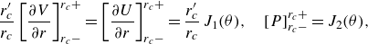 \begin{eqnarray} \frac {r_c'}{r_c}\left [\frac {\partial V}{\partial r}\right ]^{r_c+}_{r_c-} =\left [\frac {\partial U}{\partial r}\right ]^{r_c+}_{r_c-} =\frac {r_c'}{r_c}\,J_1(\theta ),\quad [P ]^{r_c+}_{r_c-}=J_2(\theta ), \end{eqnarray}
where
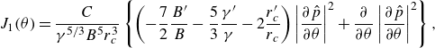 \begin{eqnarray} J_1(\theta )=\frac {C}{\gamma ^{5/3}B^5r_c^3}\left \{ \left (-\frac {7}{2}\frac {B'}{B}-\frac {5}{3}\frac {\gamma '}{\gamma }-2\frac {r_c'}{r_c}\right ) \left |\frac {\partial \hat {p}}{\partial \theta }\right |^2 +\frac {\partial }{\partial \theta }\left |\frac {\partial \hat {p}}{\partial \theta }\right |^2\right \}, \end{eqnarray}
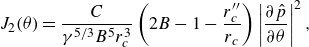 \begin{eqnarray} J_2(\theta )=\frac {C}{\gamma ^{5/3}B^5r_c^3}\left (2B-1-\frac {r_c''}{r_c} \right )\left |\frac {\partial \hat {p}}{\partial \theta }\right |^2,\end{eqnarray}
with
 $B(\theta )=1+(r_c'/r_c)^2$
,
$B(\theta )=1+(r_c'/r_c)^2$
,
 $\gamma (\theta )= ({\alpha }/{B}) ({\partial W}/{\partial r}|_{r=r_c})$
and
$\gamma (\theta )= ({\alpha }/{B}) ({\partial W}/{\partial r}|_{r=r_c})$
and
 $C=2\pi (2/3)^{2/3}\,\Gamma (1/3)\approx 12.8454$
, where
$C=2\pi (2/3)^{2/3}\,\Gamma (1/3)\approx 12.8454$
, where
 $\Gamma$
is the gamma function. The primes denote the derivatives with respect to
$\Gamma$
is the gamma function. The primes denote the derivatives with respect to
 $\theta$
. Those jump conditions play the same physical role as the Reynolds stress terms
$\theta$
. Those jump conditions play the same physical role as the Reynolds stress terms
 $F_r$
and
$F_r$
and
 $F_{\theta }$
. The fully reduced VWI closure is therefore (2.4), (3.6) and the inviscid version of (3.2). In principle, this system can be obtained by substituting the asymptotic expansions into the full equations (2.1) and performing some straightforward algebraic manipulations.
$F_{\theta }$
. The fully reduced VWI closure is therefore (2.4), (3.6) and the inviscid version of (3.2). In principle, this system can be obtained by substituting the asymptotic expansions into the full equations (2.1) and performing some straightforward algebraic manipulations.
The regularised VWI system is an APR of the fully reduced VWI, and the former system is easier to solve as we do not need to impose the jump conditions explicitly. The terms appearing in that system are a subset of those in (2.7). The nonlinear solutions of the regularised VWI system can therefore be obtained by omitting the computations of unnecessary terms in the numerical code described in § 2.2. It should also be remarked that the equations obtained by linearising the regularised VWI system around the 2-vortex solution correspond exactly to the eigenvalue problem used to compute figure 3. Therefore, by using the eigenvector of the neutral solution as the initial value for the Newton method, a nonlinear travelling wave solution can be obtained around the neutral curve.

Figure 5. Bifurcations of the VWI-type travelling wave solutions from the inviscid mode. The regularised VWI system with
 $R=10^5$
is used for computation. The bifurcation point indicated by the black dot corresponds to the same point shown in figure 3. (a) The results for fixed wavenumbers. (b) The results for fixed Dean numbers. Resolution is checked using up to
$R=10^5$
is used for computation. The bifurcation point indicated by the black dot corresponds to the same point shown in figure 3. (a) The results for fixed wavenumbers. (b) The results for fixed Dean numbers. Resolution is checked using up to
 $(L,M)=(70,50)$
. Note that in the regularised VWI, no harmonics are involved in the
$(L,M)=(70,50)$
. Note that in the regularised VWI, no harmonics are involved in the
 $z$
direction. The pink dot indicates the nonlinear solution shown in figure 6.
$z$
direction. The pink dot indicates the nonlinear solution shown in figure 6.

Figure 6. The flow structure of the VWI-type solution at
 $(K ,R, \alpha ) =(1.5 \times 10^6, 10^5, 0.1)$
, corresponding to the pink dot in figure 5. The phase speed is
$(K ,R, \alpha ) =(1.5 \times 10^6, 10^5, 0.1)$
, corresponding to the pink dot in figure 5. The phase speed is
 $c\approx 0.2597$
. (a) The vector field represents the roll velocities
$c\approx 0.2597$
. (a) The vector field represents the roll velocities
 $\overline {u}$
and
$\overline {u}$
and
 $\overline {v}$
. The colour indicates the deviation of the streak velocity
$\overline {v}$
. The colour indicates the deviation of the streak velocity
 $\overline {w}$
from that of the 2-vortex solution at the same
$\overline {w}$
from that of the 2-vortex solution at the same
 $K$
. (b) The black dashed curves represent the isocontours of
$K$
. (b) The black dashed curves represent the isocontours of
 $\overline {w}$
, while the coloured curves show the isocontours of
$\overline {w}$
, while the coloured curves show the isocontours of
 $\tilde {\omega }_z$
at
$\tilde {\omega }_z$
at
 $\varphi =0$
. (c) The red/blue surface depicts the positive/negative isosurfaces of
$\varphi =0$
. (c) The red/blue surface depicts the positive/negative isosurfaces of
 $\tilde {\omega }_z$
at magnitude
$\tilde {\omega }_z$
at magnitude
 $0.002$
. The phase is defined by
$0.002$
. The phase is defined by
 $\varphi = \alpha (z - c t)$
.
$\varphi = \alpha (z - c t)$
.
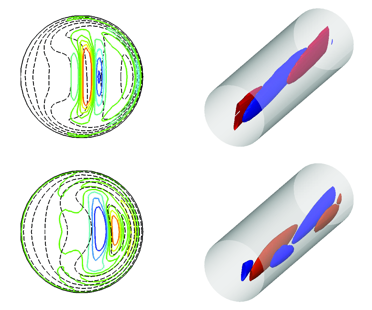
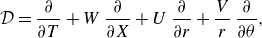
The bifurcation diagram is obtained as figure 5. The parameter range computed in the two plots corresponds to the magenta dashed lines in figure 3(b), indicating that the bifurcation is supercritical. Figure 6 shows the flow structure of the travelling wave solution at the pink dot in figure 5. Here and hereafter, in order to visualise the flow field, we adopt the flow decomposition
 $\mathbf {u}=(\overline {u},\overline {v},\overline {w})+ (\tilde u, \tilde v, \tilde w)$
, with the first term on the right-hand side representing the
$\mathbf {u}=(\overline {u},\overline {v},\overline {w})+ (\tilde u, \tilde v, \tilde w)$
, with the first term on the right-hand side representing the
 $z$
-averaged part. More specifically, we apply this decomposition for the leading-order part of the asymptotic expansions. Thus for VWI,
$z$
-averaged part. More specifically, we apply this decomposition for the leading-order part of the asymptotic expansions. Thus for VWI,
 $(\overline {u},\overline {v},\overline {w})=(R^{-1}U,R^{-1}V,W)$
, and the wave components can be used with their notation unchanged. The arrows in figure 6(a) indicate that the components
$(\overline {u},\overline {v},\overline {w})=(R^{-1}U,R^{-1}V,W)$
, and the wave components can be used with their notation unchanged. The arrows in figure 6(a) indicate that the components
 $\overline {u}$
and
$\overline {u}$
and
 $\overline {v}$
, traditionally called the ‘roll’ component in the VWI and self-sustaining process theory, inherit the large-scale swirls by the 2-vortex solution. The black contours in figure 6(b) show the ‘streak’ component,
$\overline {v}$
, traditionally called the ‘roll’ component in the VWI and self-sustaining process theory, inherit the large-scale swirls by the 2-vortex solution. The black contours in figure 6(b) show the ‘streak’ component,
 $W$
. The colour map in figure 6(a) illustrates the extent to which the component
$W$
. The colour map in figure 6(a) illustrates the extent to which the component
 $\overline {w}$
deviates from that of the 2-vortex solution. Figure 6(c) shows the three-dimensional structure of the ‘wave’ component visualised by the isosurfaces of the streamwise vorticity
$\overline {w}$
deviates from that of the 2-vortex solution. Figure 6(c) shows the three-dimensional structure of the ‘wave’ component visualised by the isosurfaces of the streamwise vorticity
 $\tilde {\omega }_z=r^{-1}( {\partial (r\tilde {v})}/{\partial r})-({\partial \tilde {u}}/{\partial \theta }))$
. Here, we switched the streamwise variable to the phase
$\tilde {\omega }_z=r^{-1}( {\partial (r\tilde {v})}/{\partial r})-({\partial \tilde {u}}/{\partial \theta }))$
. Here, we switched the streamwise variable to the phase
 $\varphi = \alpha (z - c t) \in [0,2\pi ]$
. As seen in figure 6(b), the wave structure is concentrated around the critical level, at which
$\varphi = \alpha (z - c t) \in [0,2\pi ]$
. As seen in figure 6(b), the wave structure is concentrated around the critical level, at which
 $\overline {u}$
matches the phase speed
$\overline {u}$
matches the phase speed
 $c\approx 0.2597$
. This amplification, also seen in other numerical works (Wang et al. Reference Wang, Gibson and Waleffe2007; Viswanath Reference Viswanath2009; Mckeon & Sharma Reference Mckeon and Sharma2010), is precisely due to the fact that inviscid neutral waves have singularity there. It can be shown easily that
$c\approx 0.2597$
. This amplification, also seen in other numerical works (Wang et al. Reference Wang, Gibson and Waleffe2007; Viswanath Reference Viswanath2009; Mckeon & Sharma Reference Mckeon and Sharma2010), is precisely due to the fact that inviscid neutral waves have singularity there. It can be shown easily that
 $\tilde {\omega }_z$
is
$\tilde {\omega }_z$
is
 $O(R^{-7/6})$
outside the critical layer, while inside it scales as
$O(R^{-7/6})$
outside the critical layer, while inside it scales as
 $O(R^{-1/2})$
. The flow field satisfies
$O(R^{-1/2})$
. The flow field satisfies
 \begin{equation} [u,v,w](r,\theta ,\varphi )=[u,-v,w](r,-\theta +\pi ,\varphi +\pi ). \end{equation}
This equation implies that the flow field remains unchanged when shifted by half a period in the streamwise direction and reflected about the
 $\theta =0,\pi$
axis. This symmetry is referred to as the sinuous mode in the context of secondary flow instability in boundary layer flows (Hall & Horseman Reference Hall and Horseman1991; Yu & Liu Reference Yu and Liu1994).
$\theta =0,\pi$
axis. This symmetry is referred to as the sinuous mode in the context of secondary flow instability in boundary layer flows (Hall & Horseman Reference Hall and Horseman1991; Yu & Liu Reference Yu and Liu1994).
3.3. Bifurcation from the curvature mode: BRE
A similar bifurcation analysis can be performed for the curvature mode shown in figure 4. Recall that in § 3.1, we rescaled the wavenumber and the growth rate as
 $\alpha = R^{-1}{\alpha _0}$
and
$\alpha = R^{-1}{\alpha _0}$
and
 $\sigma = R^{-1}{\sigma _0}$
. This motivates us to employ the expansions
$\sigma = R^{-1}{\sigma _0}$
. This motivates us to employ the expansions
 \begin{eqnarray} u=R^{-1}\,U(r,\theta ,X,T)+\cdots ,\quad v=R^{-1}\,V(r,\theta ,X,T)+\cdots , \end{eqnarray}
 \begin{eqnarray} w=W(r,\theta ,X,T)+\cdots , \quad p=R^{-2}\,P(r,\theta ,X,T)+\cdots , \end{eqnarray}
using
 $X=R^{-1}z$
,
$X=R^{-1}z$
,
 $T=R^{-1}t$
. Substituting these into the full Navier–Stokes equations (2.1) yields the reduced problem
$T=R^{-1}t$
. Substituting these into the full Navier–Stokes equations (2.1) yields the reduced problem
 \begin{eqnarray} \frac {\partial W}{\partial X}+\frac {\partial U}{\partial r}+\frac {U}{r}+\frac {1}{r}\,\frac {\partial V}{\partial \theta }=0, \end{eqnarray}
 \begin{eqnarray} \mathcal {D}U-\frac {V^2}{r}-\frac {K}{2}\, W^2\cos \theta =-\frac {\partial P}{\partial r}+ \Delta_2 U-\frac {U}{r^2}-\frac {2}{r^2}\,\frac {\partial V}{\partial \theta }, \end{eqnarray}
 \begin{eqnarray} \mathcal {D}V+\frac {UV}{r}+\frac {K}{2}\, W^2 \sin \theta =-\frac {1}{r}\,\frac {\partial P}{\partial \theta }+ \Delta_2 V-\frac {V}{r^2}+\frac {2}{r^2}\,\frac {\partial U}{\partial \theta }, \end{eqnarray}
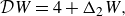 \begin{eqnarray} \mathcal {D}W=4+ \Delta _2 W, \end{eqnarray}
correct to
 $O(R^{-2})$
in the Dean limit. Here, we have defined the operator
$O(R^{-2})$
in the Dean limit. Here, we have defined the operator
 \begin{eqnarray} \mathcal {D}=\frac {\partial }{\partial T}+ W\, \frac {\partial }{\partial X} +U\,\frac {\partial }{\partial r}+\frac {V}{r}\,\frac {\partial }{\partial \theta }, \end{eqnarray}
and impose the boundary conditions
 $U=V=W=0$
at
$U=V=W=0$
at
 $r=1$
. Equations (3.9) have similar structure to the nonlinear equations for the Görtler vortex problem formulated by Hall (Reference Hall1988), and (4.2) in Smith (Reference Smith1976). These types of equations are more commonly referred to as boundary region equations (BRE) for the study of boundary layer flows (see the discussion in Wu et al. (Reference Wu, Zhao and Luo2011) and Deguchi et al. (Reference Deguchi, Hall and Walton2013)), and we will adopt this terminology. One can easily confirm that the reduced problem (2.7) is an APR of BRE.
$r=1$
. Equations (3.9) have similar structure to the nonlinear equations for the Görtler vortex problem formulated by Hall (Reference Hall1988), and (4.2) in Smith (Reference Smith1976). These types of equations are more commonly referred to as boundary region equations (BRE) for the study of boundary layer flows (see the discussion in Wu et al. (Reference Wu, Zhao and Luo2011) and Deguchi et al. (Reference Deguchi, Hall and Walton2013)), and we will adopt this terminology. One can easily confirm that the reduced problem (2.7) is an APR of BRE.

Figure 7. Bifurcations of the BRE type travelling wave solutions from the curvature mode. The solution branches are computed by (2.4) with
 $R=10^6$
. (a) The scaled wavenumber
$R=10^6$
. (a) The scaled wavenumber
 $\alpha _0=\alpha R$
is fixed. (b) The Dean number
$\alpha _0=\alpha R$
is fixed. (b) The Dean number
 $K$
is fixed. The red and green dots are the same as those in figure 4. Resolution is checked using up to
$K$
is fixed. The red and green dots are the same as those in figure 4. Resolution is checked using up to
 $(L,M,N)=(25,25,30)$
.
$(L,M,N)=(25,25,30)$
.

Figure 8. The same flow visualisation as figure 6, but for the BRE-type solution at
 $(K,\alpha _0 ,R) =(5.5 \times 10^4, 3380, 10^6)$
, corresponding to the blue dot in figure 7(a). The phase speed is
$(K,\alpha _0 ,R) =(5.5 \times 10^4, 3380, 10^6)$
, corresponding to the blue dot in figure 7(a). The phase speed is
 $c\approx 0.5033$
. In (c), the isosurfaces of
$c\approx 0.5033$
. In (c), the isosurfaces of
 $\tilde {\omega }_z=\pm 7 \times 10^{-5}$
are shown.
$\tilde {\omega }_z=\pm 7 \times 10^{-5}$
are shown.
Equations (3.9) linearised around the Dean vortex are given by (3.4). Therefore, nonlinear travelling wave solutions bifurcating from the 2-vortex can be calculated from the neutral curve of the curvature mode seen in figure 4. As seen in figure 7, the bifurcation is subcritical. The parameter range for which we calculated nonlinear solutions is indicated by the dashed lines in figure 4; these solutions exist when
 $K$
is greater than 43 086. Comparing figures 5 and 7, the BRE-type solutions, in contrast to the VWI-type solutions, show an increase in flux relative to the 2-vortex. This is because, as seen in figure 8(a), the nonlinear interaction generates high-speed streaks near the upper and lower pipe walls. The three-dimensional wave components are concentrated around the outer side of the curved pipe (figure 8
c). From figure 8(b), it can be observed that this location corresponds to the region where the streamwise velocity reaches its maximum. Despite the qualitative differences in the flow fields compared to the VWI-type, the BRE solution also satisfies the shift–reflection symmetry (3.7).
$K$
is greater than 43 086. Comparing figures 5 and 7, the BRE-type solutions, in contrast to the VWI-type solutions, show an increase in flux relative to the 2-vortex. This is because, as seen in figure 8(a), the nonlinear interaction generates high-speed streaks near the upper and lower pipe walls. The three-dimensional wave components are concentrated around the outer side of the curved pipe (figure 8
c). From figure 8(b), it can be observed that this location corresponds to the region where the streamwise velocity reaches its maximum. Despite the qualitative differences in the flow fields compared to the VWI-type, the BRE solution also satisfies the shift–reflection symmetry (3.7).
The fact that the onset of three-dimensional turbulence increases the flow rate has also been reported in numerical simulations (Noorani & Schlatter Reference Noorani and Schlatter2015) and experiments (Vester et al. Reference Vester, Örlü and Alfredsson2016).
4. Continuation from the finite-amplitude solutions in a straight pipe
4.1. Large Reynolds number limits of the exact coherent structures in a straight pipe
As already noted, when
 $K=0$
, (2.7) reduce to the straight pipe flow problem governed by the Navier–Stokes equations, for which a variety of exact coherent structures is available (Faisst & Eckhardt Reference Faisst and Eckhardt2003; Wedin & Kerswell Reference Wedin and Kerswell2004; Pringle & Kerswell Reference Pringle and Kerswell2007; Pringle et al. Reference Pringle, Duguet and Kerswell2009). Ozcakir et al. (Reference Ozcakir, Tanveer, Hall and Overman2016) confirmed that some of these exact coherent structures follow the VWI theory at sufficiently high Reynolds numbers. In this paper, we utilise the solution found by Pringle & Kerswell (Reference Pringle and Kerswell2007), which is later labelled as M1 in Pringle et al. (Reference Pringle, Duguet and Kerswell2009). This solution was not studied in Ozcakir et al. (Reference Ozcakir, Tanveer, Hall and Overman2016).
$K=0$
, (2.7) reduce to the straight pipe flow problem governed by the Navier–Stokes equations, for which a variety of exact coherent structures is available (Faisst & Eckhardt Reference Faisst and Eckhardt2003; Wedin & Kerswell Reference Wedin and Kerswell2004; Pringle & Kerswell Reference Pringle and Kerswell2007; Pringle et al. Reference Pringle, Duguet and Kerswell2009). Ozcakir et al. (Reference Ozcakir, Tanveer, Hall and Overman2016) confirmed that some of these exact coherent structures follow the VWI theory at sufficiently high Reynolds numbers. In this paper, we utilise the solution found by Pringle & Kerswell (Reference Pringle and Kerswell2007), which is later labelled as M1 in Pringle et al. (Reference Pringle, Duguet and Kerswell2009). This solution was not studied in Ozcakir et al. (Reference Ozcakir, Tanveer, Hall and Overman2016).
The solid curve in figure 9(a) shows the bifurcation diagram of the M1 solution. This solution appears at a saddle–node bifurcation, occurring at the lowest flux-based Reynolds number
 $2RQ\approx 773$
among all known solutions. In the laminar parabolic profile, the value of
$2RQ\approx 773$
among all known solutions. In the laminar parabolic profile, the value of
 $Q$
is 0.5, and under constant pressure, nonlinear effects should decrease the flux. Therefore, the upper curve in the figure corresponds to the ‘lower branch solutions’ referred to in previous literature. As shown in Pringle & Kerswell (Reference Pringle and Kerswell2007), the solution possesses mirror symmetry with respect to the line
$Q$
is 0.5, and under constant pressure, nonlinear effects should decrease the flux. Therefore, the upper curve in the figure corresponds to the ‘lower branch solutions’ referred to in previous literature. As shown in Pringle & Kerswell (Reference Pringle and Kerswell2007), the solution possesses mirror symmetry with respect to the line
 $\theta =\pm \pi /2$
,
$\theta =\pm \pi /2$
,
 \begin{equation} [u,v,w](r,\theta ,\varphi )=[u,-v,w](r,-\theta +\pi ,\varphi ), \end{equation}
and the shift–reflection symmetry with respect to the line
 $\theta =0,\pi$
,
$\theta =0,\pi$
,
 \begin{equation} [u,v,w](r,\theta ,\varphi )=[u,-v,w](r,-\theta ,\varphi +\pi ). \end{equation}
Due to the symmetry of the system, arbitrary shifts in the
 $\theta$
and
$\theta$
and
 $z$
directions do not disqualify M1 as a solution. However, when the effect of pipe curvature is introduced, the orientation in the
$z$
directions do not disqualify M1 as a solution. However, when the effect of pipe curvature is introduced, the orientation in the
 $\theta$
direction is no longer arbitrary. In this study, we use both the original orientation from Pringle & Kerswell (Reference Pringle and Kerswell2007) and an orientation rotated by
$\theta$
direction is no longer arbitrary. In this study, we use both the original orientation from Pringle & Kerswell (Reference Pringle and Kerswell2007) and an orientation rotated by
 $90^\circ$
in the
$90^\circ$
in the
 $\theta$
direction. Figure 10(a) shows the flow field for the latter orientation at
$\theta$
direction. Figure 10(a) shows the flow field for the latter orientation at
 $R=40\,000$
, where mirror symmetry and shift–reflection symmetry become
$R=40\,000$
, where mirror symmetry and shift–reflection symmetry become
 \begin{equation} [u,v,w](r,\theta ,\varphi )=[u,-v,w](r,-\theta ,\varphi ) \end{equation}
and (3.7), respectively. Since the wavenumber
 $\alpha$
is fixed in figure 9(a), the solution branch is expected to converge to the VWI results at high Reynolds numbers. To verify this, we used the Navier–Stokes solution at
$\alpha$
is fixed in figure 9(a), the solution branch is expected to converge to the VWI results at high Reynolds numbers. To verify this, we used the Navier–Stokes solution at
 $R=4\times 10^4$
as the initial condition for the regularised VWI code. The converged solution, shown in figure 10(b), is almost indistinguishable from the initial condition, figure 10(a). The dashed curve in figure 9(a) represents the regularised VWI results, which provide an excellent approximation when
$R=4\times 10^4$
as the initial condition for the regularised VWI code. The converged solution, shown in figure 10(b), is almost indistinguishable from the initial condition, figure 10(a). The dashed curve in figure 9(a) represents the regularised VWI results, which provide an excellent approximation when
 $R$
is
$R$
is
 $O(10^4)$
or larger.
$O(10^4)$
or larger.
We can also compute the BRE limit of the M1 solution following Deguchi et al. (Reference Deguchi, Hall and Walton2013), where this limit was first applied for exact coherent structures in the context of plane Couette flow. The main idea is switching the parameters
 $(R,\alpha )$
to
$(R,\alpha )$
to
 $({\alpha _0},\epsilon )$
, where
$({\alpha _0},\epsilon )$
, where
 $\epsilon =R^{-2}$
, and reformulating the problem as a regular perturbation problem. The limit as
$\epsilon =R^{-2}$
, and reformulating the problem as a regular perturbation problem. The limit as
 $\epsilon \rightarrow 0$
then corresponds to the BRE; see Appendix A for more detail.
$\epsilon \rightarrow 0$
then corresponds to the BRE; see Appendix A for more detail.

Figure 9. Continuation of the M1 straight pipe flow solution found by Pringle & Kerswell (Reference Pringle and Kerswell2007). (a) Results with a fixed wavenumber
 $\alpha =1.44$
. The solid curve is the solution of the Navier–Stokes equations with
$\alpha =1.44$
. The solid curve is the solution of the Navier–Stokes equations with
 $(L,M,N)=(70,50,6)$
. The dashed curve shows the regularised VWI results with
$(L,M,N)=(70,50,6)$
. The dashed curve shows the regularised VWI results with
 $(L,M)=(70,50)$
. (b) Results with a fixed scaled wavenumber
$(L,M)=(70,50)$
. (b) Results with a fixed scaled wavenumber
 $ \alpha _0=\alpha R=1728$
. The horizontal axis is
$ \alpha _0=\alpha R=1728$
. The horizontal axis is
 $\epsilon =R^{-2}$
. The black curve and the red points correspond to the resolution levels
$\epsilon =R^{-2}$
. The black curve and the red points correspond to the resolution levels
 $(L,M,N)=(50,22,24)$
and
$(L,M,N)=(50,22,24)$
and
 $(30,22,18)$
, respectively.
$(30,22,18)$
, respectively.
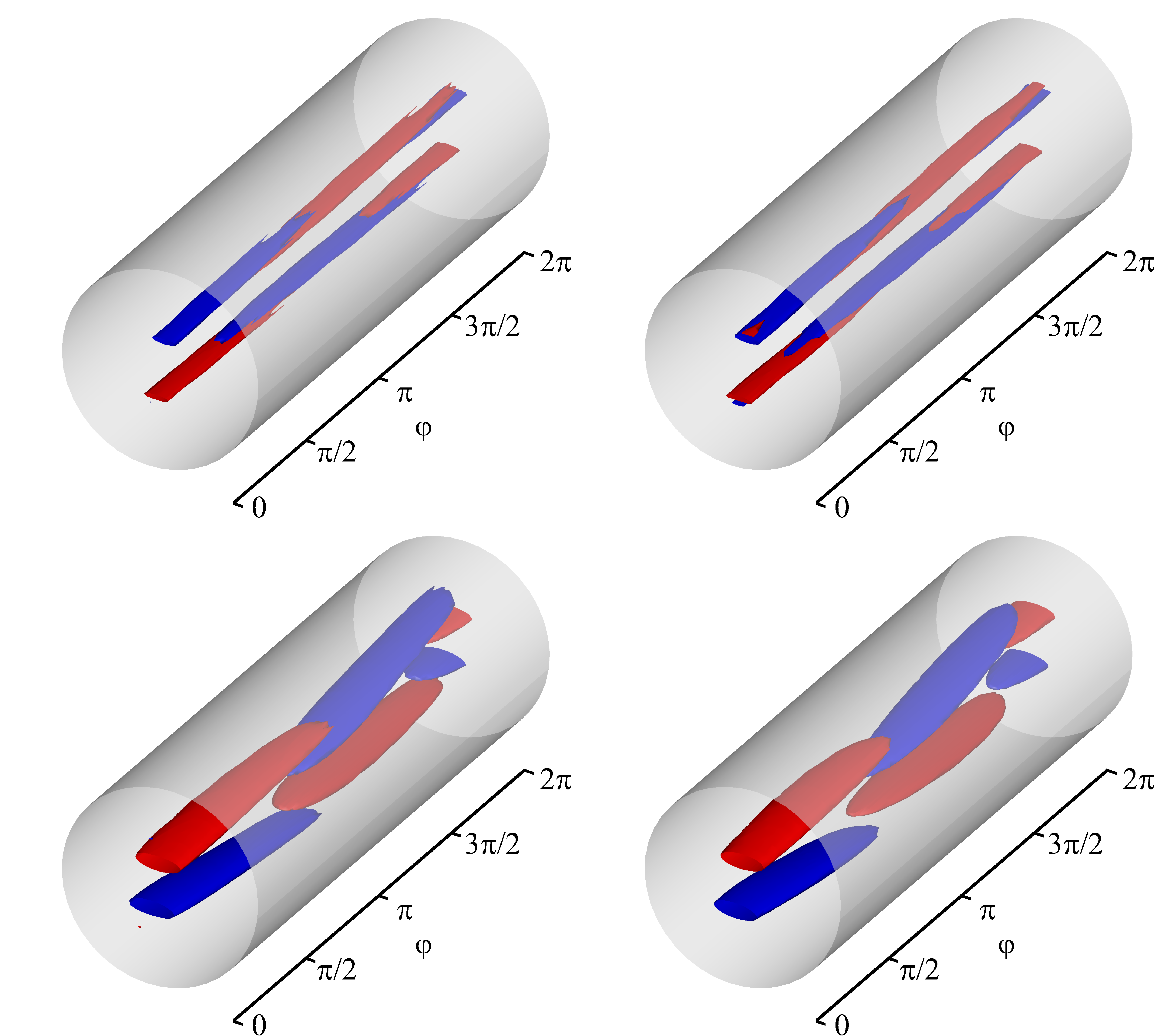
Figure 10. The three-dimensional structure of the M1 solutions at the VWI and BRE limits. The same format as figure 6(c), but for
 $\tilde {\omega }_z= \pm 0.02$
. (a) The Navier–Stokes result at
$\tilde {\omega }_z= \pm 0.02$
. (a) The Navier–Stokes result at
 $(\alpha , R)=(1.44,4 \times 10^4)$
. (b) The regularised VWI result at
$(\alpha , R)=(1.44,4 \times 10^4)$
. (b) The regularised VWI result at
 $(\alpha , R)=(1.44,4 \times 10^4)$
. (c) The Navier–Stokes result at
$(\alpha , R)=(1.44,4 \times 10^4)$
. (c) The Navier–Stokes result at
 $( \alpha _0, R)=(1728, 10^4)$
. (d) The BRE result at
$( \alpha _0, R)=(1728, 10^4)$
. (d) The BRE result at
 $ \alpha _0=1728$
(i.e. formally
$ \alpha _0=1728$
(i.e. formally
 $R=\infty$
). The isosurfaces are the asymptotic prediction at
$R=\infty$
). The isosurfaces are the asymptotic prediction at
 $R=10^4$
, showing the wave part of
$R=10^4$
, showing the wave part of
 $10^{-4}r^{-1}( ({\partial (rV)}/{\partial r})- ({\partial U}/{\partial \theta }))$
.
$10^{-4}r^{-1}( ({\partial (rV)}/{\partial r})- ({\partial U}/{\partial \theta }))$
.
The solid curve in figure 9(b) represents the same M1 solution as in figure 9(a), but with
 $\alpha _0$
fixed and
$\alpha _0$
fixed and
 $\epsilon$
reduced. This computation, which employs a resolution deemed more than sufficient, encounters numerical instability, with the condition number of the Jacobian matrix deteriorating rapidly as
$\epsilon$
reduced. This computation, which employs a resolution deemed more than sufficient, encounters numerical instability, with the condition number of the Jacobian matrix deteriorating rapidly as
 $\epsilon$
decreases. This issue is somewhat expected, given that the limit involves an infinite Reynolds number and infinitely long pipe. Lowering the resolution mitigates this issue (see the red circles in figure 9
b), allowing the solution to even reach
$\epsilon$
decreases. This issue is somewhat expected, given that the limit involves an infinite Reynolds number and infinitely long pipe. Lowering the resolution mitigates this issue (see the red circles in figure 9
b), allowing the solution to even reach
 $\epsilon =0$
. Figure 10(c) shows the high-resolution computation at
$\epsilon =0$
. Figure 10(c) shows the high-resolution computation at
 $\epsilon =10^{-8}$
(
$\epsilon =10^{-8}$
(
 $R=10^4$
), while figure 10(d
) presents the asymptotic prediction made at
$R=10^4$
), while figure 10(d
) presents the asymptotic prediction made at
 $R=10^4$
using the low-resolution result at
$R=10^4$
using the low-resolution result at
 $\epsilon =0$
. Both results match closely, demonstrating that the use of
$\epsilon =0$
. Both results match closely, demonstrating that the use of
 $\epsilon =10^{-8}$
serves as a sufficiently accurate approximation of the BRE solution.
$\epsilon =10^{-8}$
serves as a sufficiently accurate approximation of the BRE solution.
4.2. Continuation from the VWI mode
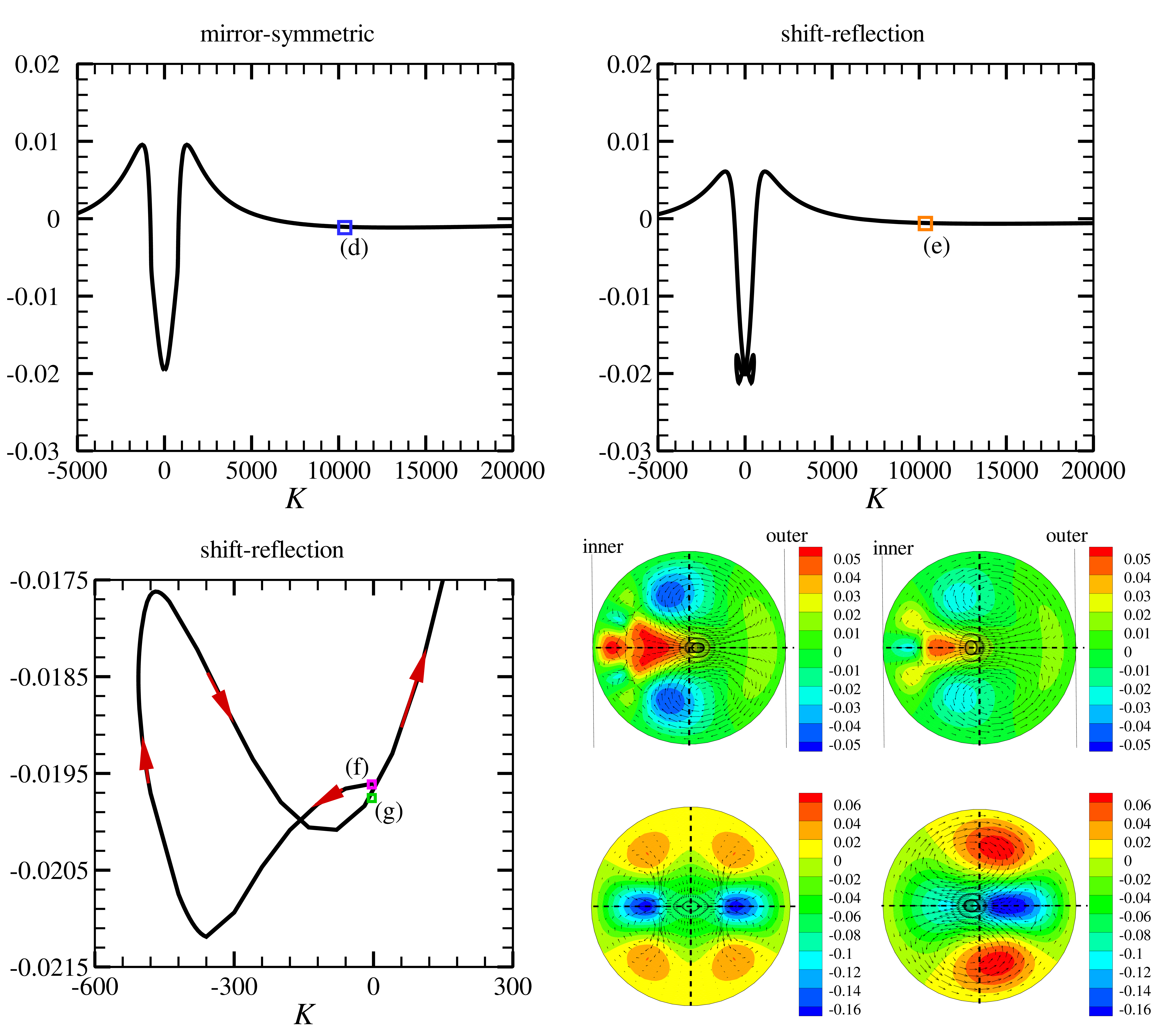
Figure 11. Continuation from the VWI-type straight pipe flow solution (see figure 9
a). The regularised VWI with
 $(\alpha ,R)=(1.44,4\times 10^4)$
is used. Resolution is checked using up to
$(\alpha ,R)=(1.44,4\times 10^4)$
is used. Resolution is checked using up to
 $(L,M)=(70,50)$
. (a) The continuation from the rotated orientation shown in figure 10(b). The solution has mirror symmetry (4.2). (b) The continuation from the original orientation. The solution has shift–reflection symmetry (4.3). (c) The same result as in (b), but enlarged around
$(L,M)=(70,50)$
. (a) The continuation from the rotated orientation shown in figure 10(b). The solution has mirror symmetry (4.2). (b) The continuation from the original orientation. The solution has shift–reflection symmetry (4.3). (c) The same result as in (b), but enlarged around
 $K=0$
. (d–g) Flow visualisation at the corresponding points on the bifurcation diagrams. The format is the same as in figure 6(a).
$K=0$
. (d–g) Flow visualisation at the corresponding points on the bifurcation diagrams. The format is the same as in figure 6(a).
Now let us add the effect of pipe curvature to the VWI mode obtained in figure 9(a). Starting from the configuration shown in figure 10(b) (i.e. rotated by
 $90^\circ$
from the original orientation), mirror symmetry is preserved, while shift–reflection symmetry is broken. As shown in figure 11(a), introducing a small curvature causes the value of
$90^\circ$
from the original orientation), mirror symmetry is preserved, while shift–reflection symmetry is broken. As shown in figure 11(a), introducing a small curvature causes the value of
 $\Delta Q$
to increase. As
$\Delta Q$
to increase. As
 $K$
increases further,
$K$
increases further,
 $\Delta Q$
decreases and approaches zero. We can extend the branch to values of
$\Delta Q$
decreases and approaches zero. We can extend the branch to values of
 $K$
where the linear instabilities are observed in § 3.1. However, no connection to the 2-vortex solution was detected.
$K$
where the linear instabilities are observed in § 3.1. However, no connection to the 2-vortex solution was detected.
The black dashed contours in figure 12(a) illustrate the streak component
 $\overline {w}$
at
$\overline {w}$
at
 $K=10\,000$
(indicated by the blue square in figure 11
a). The flow structure is overall similar to that for the 2-vortex solution at the same parameter; see figure 12(c). The difference between those two fields, presented in figure 11(d), reveals that changes in the streak due to three-dimensional effects occur primarily near the inner wall, contrasting with the observations in figures 6 and 8. The amplitude of the wave component responsible for this mechanism is strongest at the critical layer, as expected for VWI-type exact coherent structures (see the coloured contours in figure 12
a).
$K=10\,000$
(indicated by the blue square in figure 11
a). The flow structure is overall similar to that for the 2-vortex solution at the same parameter; see figure 12(c). The difference between those two fields, presented in figure 11(d), reveals that changes in the streak due to three-dimensional effects occur primarily near the inner wall, contrasting with the observations in figures 6 and 8. The amplitude of the wave component responsible for this mechanism is strongest at the critical layer, as expected for VWI-type exact coherent structures (see the coloured contours in figure 12
a).
If the original orientation (see figure 11
f) is used as the starting point of the continuation, then the solution retains shift–reflection symmetry, but mirror symmetry is lost. The resulting bifurcation diagram, shown in figure 11(b), is similar to the previous one, except for the complex structure observed near
 $K=0$
. Figure 11(c) is the enlargement of this part, where one of the symmetric branches has been omitted for clarity. Starting from the M1 solution, the solution branch extending into the negative
$K=0$
. Figure 11(c) is the enlargement of this part, where one of the symmetric branches has been omitted for clarity. Starting from the M1 solution, the solution branch extending into the negative
 $K$
region forms a loop and reaches the
$K$
region forms a loop and reaches the
 $K=0$
axis again. At this point, the solution retains shift–reflection symmetry but lacks mirror symmetry. The flow field of this solution (figure 11
g) closely resembles that of the asymmetric solution reported by Pringle & Kerswell (Reference Pringle and Kerswell2007), referred to as S1 in Pringle et al. (Reference Pringle, Duguet and Kerswell2009).
$K=0$
axis again. At this point, the solution retains shift–reflection symmetry but lacks mirror symmetry. The flow field of this solution (figure 11
g) closely resembles that of the asymmetric solution reported by Pringle & Kerswell (Reference Pringle and Kerswell2007), referred to as S1 in Pringle et al. (Reference Pringle, Duguet and Kerswell2009).
The solution branch appears to continue indefinitely towards large
 $K$
, but once again, no direct connection to Dean vortices is observed. The deviation of the streamwise velocity from the 2-vortex at
$K$
, but once again, no direct connection to Dean vortices is observed. The deviation of the streamwise velocity from the 2-vortex at
 $K=10\,000$
, shown in figure 11(e), is qualitatively similar to that in figure 11(d). A strong vortex layer appears in the wave component at the critical level, as shown in figure 12(b). Although the structural details of the coloured contour differ from that in figure 12(a), the physical role that waves play seems to be the same.
$K=10\,000$
, shown in figure 11(e), is qualitatively similar to that in figure 11(d). A strong vortex layer appears in the wave component at the critical level, as shown in figure 12(b). Although the structural details of the coloured contour differ from that in figure 12(a), the physical role that waves play seems to be the same.
Figure 12. Contours of the streak (black dashed lines) and the wave vorticity (coloured solid lines). The same format as figure 6(b). Here,
 $K=10^4$
. (a) The mirror-symmetric solution shown in figure 11(d). The phase speed is
$K=10^4$
. (a) The mirror-symmetric solution shown in figure 11(d). The phase speed is
 $c\approx 0.3031$
. (b) The shift–reflection-symmetric solution shown in figure 11(e). The phase speed is
$c\approx 0.3031$
. (b) The shift–reflection-symmetric solution shown in figure 11(e). The phase speed is
 $c\approx 0.3302$
. (c) The 2-vortex solution.
$c\approx 0.3302$
. (c) The 2-vortex solution.
4.3. Continuation from the BRE mode
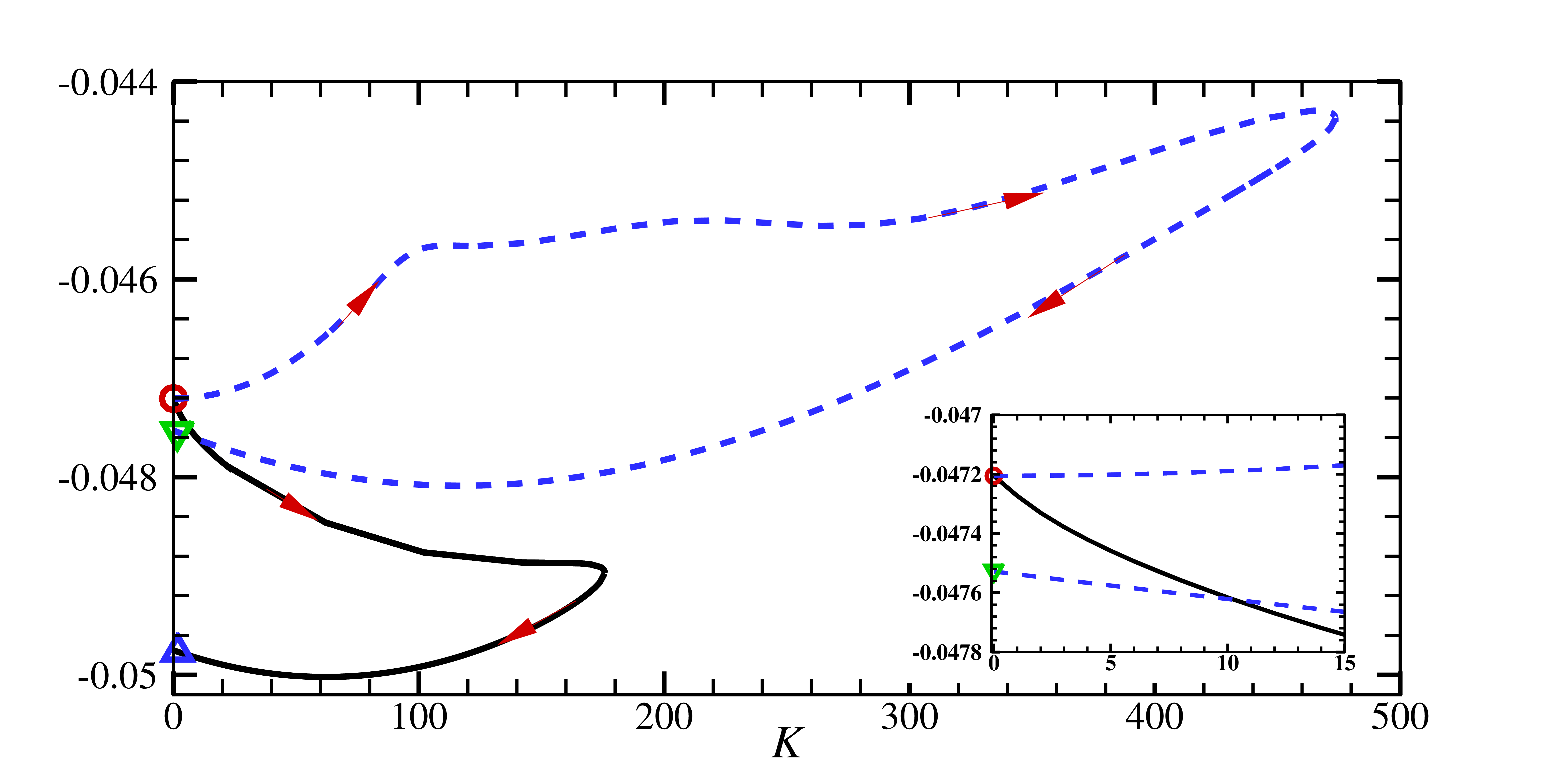
Figure 13. Continuation from the BRE-type straight pipe flow solution (see figure 9
b). Equations (2.7) are used with
 $( \alpha _0,R)=(1728,10^4)$
. Resolution is checked using up to
$( \alpha _0,R)=(1728,10^4)$
. Resolution is checked using up to
 $(L,M,N)=(50,22,24)$
. The continuation starts from the M1 solution indicated by the circle. The solid black curve shows the continuation from the rotated orientation shown in figure 10(c). Along the curve, mirror symmetry is preserved. The dashed blue curve illustrates the continuation from the original orientation. Along the curve, shift–reflection symmetry is preserved.
$(L,M,N)=(50,22,24)$
. The continuation starts from the M1 solution indicated by the circle. The solid black curve shows the continuation from the rotated orientation shown in figure 10(c). Along the curve, mirror symmetry is preserved. The dashed blue curve illustrates the continuation from the original orientation. Along the curve, shift–reflection symmetry is preserved.
For completeness, we also examine the effect of curvature on the BRE-type solution. The black curve in figure 13 represents the bifurcation diagram starting from the M1 solution rotated by
 $90^\circ$
(indicated by the circle). Along the solution branch, similar to figure 11(a) for the VWI computation, mirror symmetry with respect to the
$90^\circ$
(indicated by the circle). Along the solution branch, similar to figure 11(a) for the VWI computation, mirror symmetry with respect to the
 $\phi =0,\pi$
axis is preserved. However, unlike the VWI case, a turning point is reached at relatively small
$\phi =0,\pi$
axis is preserved. However, unlike the VWI case, a turning point is reached at relatively small
 $K$
, after which the solution branch returns to
$K$
, after which the solution branch returns to
 $K=0$
(upward triangle). The straight pipe flow solution found at this point is not M1 but belongs to a previously unreported class of solutions that retain mirror symmetry but lack shift–reflection symmetry. Nevertheless, as shown in figures 14(a–c), the overall flow structure is not significantly different from M1. It is possible to continue the solution branch further from the new solution; however, the behaviour of the solution branch is somewhat complicated, so it is not shown in the figure.
$K=0$
(upward triangle). The straight pipe flow solution found at this point is not M1 but belongs to a previously unreported class of solutions that retain mirror symmetry but lack shift–reflection symmetry. Nevertheless, as shown in figures 14(a–c), the overall flow structure is not significantly different from M1. It is possible to continue the solution branch further from the new solution; however, the behaviour of the solution branch is somewhat complicated, so it is not shown in the figure.
The blue curve in figure 13 represents a similar computation, but initiated from the original orientation of M1. Throughout the computation, the shift–reflection symmetry is preserved. Again, the solution branch returns to the straight pipe (downward triangle). As shown in figures 14(d–f), the flow field at this point closely resembles the S1 solution. While the solution branch can be further continued, it is unlikely that it can be extended for large
 $K$
.
$K$
.

Figure 14. The asymmetric solutions obtained at
 $K=0$
in figure 13. The same format as figure 6. (c,f) The isosurface at
$K=0$
in figure 13. The same format as figure 6. (c,f) The isosurface at
 $|\tilde {\omega }_z|= 0.02$
. (a–c) The solution at the upward triangle. The phase speed is
$|\tilde {\omega }_z|= 0.02$
. (a–c) The solution at the upward triangle. The phase speed is
 $c\approx 0.6725$
. (d–f) The solution at the downward triangle. The phase speed is
$c\approx 0.6725$
. (d–f) The solution at the downward triangle. The phase speed is
 $c\approx 0.6938$
.
$c\approx 0.6938$
.
5. Conclusion and discussions
In this study, we revisited the high Reynolds number limit in a weakly curved pipe, as originally considered by Dean (Reference Dean1927, Reference Dean1928), adopting the same definition of the Dean number
 $K$
. Dean’s works and many subsequent studies employed the nonlinear equations (2.4), which are independent of
$K$
. Dean’s works and many subsequent studies employed the nonlinear equations (2.4), which are independent of
 $z$
and
$z$
and
 $t$
. We extended this result to account for three-dimensional travelling waves propagating downstream. Our approach is based on rational asymptotic analysis of the governing equations (2.1). The appropriate leading-order problem depends on how the axial wavenumber
$t$
. We extended this result to account for three-dimensional travelling waves propagating downstream. Our approach is based on rational asymptotic analysis of the governing equations (2.1). The appropriate leading-order problem depends on how the axial wavenumber
 $\alpha$
is scaled. We identified at least two distinct asymptotic states based on the suitable choices of this scaling.
$\alpha$
is scaled. We identified at least two distinct asymptotic states based on the suitable choices of this scaling.
If
 $\alpha$
is fixed while taking the high Reynolds number limit, then the leading-order problem can be formulated by combining the VWI theory with the Dean problem. More specifically, the rigorous asymptotic limit of this type is described by a system of equations that couples Dean’s equation (2.4) with a Rayleigh equation for the streak component, through the jump conditions (3.6). However, from a computational perspective, it is more practical to use a system known as the regularised VWI, which replaces the Rayleigh equation and the jump conditions with the Orr–Sommerfeld equation and the Reynolds stress terms (3.5). The justification for using the regularised VWI is that it serves as the asymptotic preserved reduction (APR) of VWI, in the sense defined in § 2.2.
$\alpha$
is fixed while taking the high Reynolds number limit, then the leading-order problem can be formulated by combining the VWI theory with the Dean problem. More specifically, the rigorous asymptotic limit of this type is described by a system of equations that couples Dean’s equation (2.4) with a Rayleigh equation for the streak component, through the jump conditions (3.6). However, from a computational perspective, it is more practical to use a system known as the regularised VWI, which replaces the Rayleigh equation and the jump conditions with the Orr–Sommerfeld equation and the Reynolds stress terms (3.5). The justification for using the regularised VWI is that it serves as the asymptotic preserved reduction (APR) of VWI, in the sense defined in § 2.2.
If the product of
 $\alpha$
and the Reynolds number is fixed during the limiting process, then the leading-order system is given by (3.9), which represents the BRE with additional curvature terms included. However, numerical instability present in this limit, especially at high resolution, makes it preferable to use the augmented system (2.7) at small
$\alpha$
and the Reynolds number is fixed during the limiting process, then the leading-order system is given by (3.9), which represents the BRE with additional curvature terms included. However, numerical instability present in this limit, especially at high resolution, makes it preferable to use the augmented system (2.7) at small
 $\epsilon =R^{-2}$
for computations. The validity of this approach is supported by the fact that (2.7) is the APR of (3.9). Moreover, since (2.7) retains all the necessary terms for the regularised VWI, it also serves as the APR of VWI. In this study, we used either (2.7) or the regularised VWI ((2.4) and (3.2) coupled by the stress body force term (3.5)) for numerical computations.
$\epsilon =R^{-2}$
for computations. The validity of this approach is supported by the fact that (2.7) is the APR of (3.9). Moreover, since (2.7) retains all the necessary terms for the regularised VWI, it also serves as the APR of VWI. In this study, we used either (2.7) or the regularised VWI ((2.4) and (3.2) coupled by the stress body force term (3.5)) for numerical computations.

Figure 15. A schematic summarising the bifurcations of the nonlinear solutions obtained in this study. The red dashed line represents the 2-vortex solution. The blue solid lines represent computations using the asymptotic problem APR of the VWI (the regularised VWI), while the purple dashed lines correspond to computations using the APR of the BRE (2.7).
Our numerical results are summarised in the sketch shown in figure 15. In § 3, we obtained nonlinear travelling wave solutions through bifurcation analysis from the Dean vortices. This approach begins with the linear stability analysis of the 2-vortex solution (§ 3.1), which corresponds to the asymptotic limit of the neutral curve obtained by Canton et al. (Reference Canton, Schlatter and Örlü2016). The instability detected by the Orr–Sommerfeld equation has an inviscid limit, from which VWI-type solutions undergo supercritical bifurcation. Given the flow characteristics and the nature of the bifurcation, this mode is likely part of the same family of supercritical travelling wave solutions as those identified by Canton et al. (Reference Canton, Rinaldi, Örlü and Schlatter2020) at moderate curvature.
We also identified another linear instability, termed the curvature mode. This mode has long wavelengths and cannot be detected by the Orr–Sommerfeld equation. As the Dean number
 $K$
increases from zero, the curvature mode emerges first at
$K$
increases from zero, the curvature mode emerges first at
 $K\approx 5.72 \times 10^4$
, followed by the onset of instability detected by the Orr–Sommerfeld equation at
$K\approx 5.72 \times 10^4$
, followed by the onset of instability detected by the Orr–Sommerfeld equation at
 $K\approx 7.78 \times 10^5$
. The former critical Dean number agrees well with the recent full Navier–Stokes results from Lupi et al. (Reference Lupi, Canton, Rinaldi, Örlü and Schlatter2024), and this is only slightly higher than the value at which the first 4-vortex solution appears,
$K\approx 7.78 \times 10^5$
. The former critical Dean number agrees well with the recent full Navier–Stokes results from Lupi et al. (Reference Lupi, Canton, Rinaldi, Örlü and Schlatter2024), and this is only slightly higher than the value at which the first 4-vortex solution appears,
 $K\approx 5.71 \times 10^4$
. The nonlinear solutions that bifurcate subcritically from the curvature mode are described by the BRE and exist when
$K\approx 5.71 \times 10^4$
. The nonlinear solutions that bifurcate subcritically from the curvature mode are described by the BRE and exist when
 $K$
exceeds
$K$
exceeds
 $4.33 \times 10^4$
.
$4.33 \times 10^4$
.
The two types of travelling wave solutions mentioned above exhibit distinct physical characteristics. First, the VWI-type solution reduces the flow rate, while the BRE-type solution increases it. Second, the Strouhal number
 $St=2\alpha c/Q$
is
$St=2\alpha c/Q$
is
 $O(1)$
for the VWI-type solution, while for the BRE-type solution, it is much smaller, of the order of
$O(1)$
for the VWI-type solution, while for the BRE-type solution, it is much smaller, of the order of
 $O(1/R)$
. The Strouhal number here is defined in the same way as in the review by Vester et al. (Reference Vester, Örlü and Alfredsson2016), and it is frequently used to quantitatively investigate the swirl-switching phenomenon of Dean vortices. Finally, we note the connection to recent efforts to extend the concept of the self-sustaining process to Taylor–Couette flow, which also involves the shear-Coriolis instability. In this context, the supercritical process proposed by Dessup et al. (Reference Dessup, Tuckerman, Wesfreid, Barkley and Willis2018) aligns with our VWI-type solution, while the subcritical process identified by Wang et al. (Reference Wang, Ayats, Deguchi, Mellibovsky and Meseguer2022) is more suitable for our BRE-type solution.
$O(1/R)$
. The Strouhal number here is defined in the same way as in the review by Vester et al. (Reference Vester, Örlü and Alfredsson2016), and it is frequently used to quantitatively investigate the swirl-switching phenomenon of Dean vortices. Finally, we note the connection to recent efforts to extend the concept of the self-sustaining process to Taylor–Couette flow, which also involves the shear-Coriolis instability. In this context, the supercritical process proposed by Dessup et al. (Reference Dessup, Tuckerman, Wesfreid, Barkley and Willis2018) aligns with our VWI-type solution, while the subcritical process identified by Wang et al. (Reference Wang, Ayats, Deguchi, Mellibovsky and Meseguer2022) is more suitable for our BRE-type solution.
In § 4, we introduced curvature effects to the M1 solution, originally found by Pringle & Kerswell (Reference Pringle and Kerswell2007) for straight pipes (i.e.
 $K=0$
). In § 4.1, we confirmed that this solution has a high Reynolds number asymptotic limit of VWI (BRE) type when
$K=0$
). In § 4.1, we confirmed that this solution has a high Reynolds number asymptotic limit of VWI (BRE) type when
 $\alpha$
(
$\alpha$
(
 $\alpha _0=\alpha R$
) is fixed. In §§ 4.2 and 4.3, the effect of pipe curvature on those limits is examined. Computational results for non-zero
$\alpha _0=\alpha R$
) is fixed. In §§ 4.2 and 4.3, the effect of pipe curvature on those limits is examined. Computational results for non-zero
 $K$
depend on how the initial M1 solution at
$K$
depend on how the initial M1 solution at
 $K=0$
is shifted in the azimuthal direction. The M1 solution possesses both mirror symmetry and shift–reflection symmetry, but their axes are orthogonal to each other. Starting the calculations from the orientation used by Pringle & Kerswell (Reference Pringle and Kerswell2007) and from a
$K=0$
is shifted in the azimuthal direction. The M1 solution possesses both mirror symmetry and shift–reflection symmetry, but their axes are orthogonal to each other. Starting the calculations from the orientation used by Pringle & Kerswell (Reference Pringle and Kerswell2007) and from a
 $90^\circ$
rotated orientation leads to different symmetries being preserved.
$90^\circ$
rotated orientation leads to different symmetries being preserved.
We found that, in general, the branches of the VWI-type solutions can be extended to large values of
 $K$
, whereas those for the BRE-type do not exhibit the same behaviour. The VWI branch approaches the 2-vortex solution as
$K$
, whereas those for the BRE-type do not exhibit the same behaviour. The VWI branch approaches the 2-vortex solution as
 $K$
increases. However, even when the branch enters the region where the 2-vortex solution becomes unstable, we could not identify a bifurcation point connecting the two solutions. An intensive parameter search (not shown in this paper) concludes that there is no apparent connection between the three-dimensional instability of the 2-vortex solution and the self-sustained solutions in the straight pipe. This is quite different from plane Couette flow studied by Nagata (Reference Nagata1988, Reference Nagata1990), where the three-dimensional solution generated by adding system rotation can be continued back to the zero-rotation limit. We note that Barnes & Kerswell (Reference Barnes and Kerswell2000) reported similar difficulties in their study of pipe flow when secondary flow is induced by system rotation.
$K$
increases. However, even when the branch enters the region where the 2-vortex solution becomes unstable, we could not identify a bifurcation point connecting the two solutions. An intensive parameter search (not shown in this paper) concludes that there is no apparent connection between the three-dimensional instability of the 2-vortex solution and the self-sustained solutions in the straight pipe. This is quite different from plane Couette flow studied by Nagata (Reference Nagata1988, Reference Nagata1990), where the three-dimensional solution generated by adding system rotation can be continued back to the zero-rotation limit. We note that Barnes & Kerswell (Reference Barnes and Kerswell2000) reported similar difficulties in their study of pipe flow when secondary flow is induced by system rotation.
When
 $K$
is smaller than
$K$
is smaller than
 $5.71\times 10^4$
, the 2-vortex solution is linearly stable, therefore the transition to turbulence must be subcritical. Interestingly, figures 7 and 11 suggest that in this regime, emergence of certain finite-amplitude travelling waves, which may support turbulent activity, result in a positive value of
$5.71\times 10^4$
, the 2-vortex solution is linearly stable, therefore the transition to turbulence must be subcritical. Interestingly, figures 7 and 11 suggest that in this regime, emergence of certain finite-amplitude travelling waves, which may support turbulent activity, result in a positive value of
 $\Delta Q$
; i.e. under the same pressure, the flow rate achieved is higher than that of the laminar flow (the 2-vortex solution). This implies that the so-called sub-laminar drag reported in previous numerical computations and experiments (see Noorani & Schlatter Reference Noorani and Schlatter2015; Vester et al. Reference Vester, Örlü and Alfredsson2016) is indeed realised for some exact coherent structures. That said, for all computations in this paper, the normalised flux
$\Delta Q$
; i.e. under the same pressure, the flow rate achieved is higher than that of the laminar flow (the 2-vortex solution). This implies that the so-called sub-laminar drag reported in previous numerical computations and experiments (see Noorani & Schlatter Reference Noorani and Schlatter2015; Vester et al. Reference Vester, Örlü and Alfredsson2016) is indeed realised for some exact coherent structures. That said, for all computations in this paper, the normalised flux
 $Q$
is always less than 0.5, which is the value for the laminar parabolic profile in the straight pipe. This result is consistent with the earlier observations.
$Q$
is always less than 0.5, which is the value for the laminar parabolic profile in the straight pipe. This result is consistent with the earlier observations.
Our numerical results show that for large
 $K$
, the three-dimensional components do not significantly affect the flow rate. The dominance of momentum transport by Taylor–Görtler–Dean vortices is likely a general feature of shear flows subjected to centrifugal instability (cf. Deguchi Reference Deguchi2023). However, in general, the three-dimensionality of the flow significantly alters the topology of the streamlines, thus our three-dimensional travelling wave solutions may be useful for studying particle transport in curved pipe flows.
$K$
, the three-dimensional components do not significantly affect the flow rate. The dominance of momentum transport by Taylor–Görtler–Dean vortices is likely a general feature of shear flows subjected to centrifugal instability (cf. Deguchi Reference Deguchi2023). However, in general, the three-dimensionality of the flow significantly alters the topology of the streamlines, thus our three-dimensional travelling wave solutions may be useful for studying particle transport in curved pipe flows.
Acknowledgements.
This research was supported by the Australian Research Council Discovery Project DP230102188.
Declaration of interests.
The authors report no conflict of interest.
Appendix A. The computation of the BRE limit
Applying the transformations
 $X=R^{-1}z$
,
$X=R^{-1}z$
,
 $T=R^{-1}t$
,
$T=R^{-1}t$
,
 $(u,v,w)=(R^{-1}U,R^{-1}V,W)$
, system (2.7) becomes
$(u,v,w)=(R^{-1}U,R^{-1}V,W)$
, system (2.7) becomes
 \begin{eqnarray} \frac {\partial W}{\partial X}+\frac {\partial U}{\partial r}+\frac {U}{r}+\frac {1}{r}\,\frac {\partial V}{\partial \theta }=0,\,\,\, \end{eqnarray}
 \begin{eqnarray} \mathcal {D}U-r^{-1}V^2- \frac {K}{2}\, W^2 \cos \theta = -\frac {\partial P}{\partial r}+ \Delta U-r^{-2}U-2r^{-2}\,\frac {\partial V}{\partial \theta }, \end{eqnarray}
 \begin{eqnarray} \mathcal {D}V+r^{-1}UV+ \frac {K}{2} W^2 \sin \theta =-r^{-1}\frac {\partial P}{\partial \theta }+\Delta V -r^{-2}V+2r^{-2}\frac {\partial U}{\partial \theta }, \end{eqnarray}
 \begin{eqnarray} \mathcal {D}W=-\epsilon\, \frac {\partial P}{\partial X}+4+\Delta W, \end{eqnarray}
where
 $\mathcal {D}=\partial _T+U\,\partial _r+r^{-1}V\,\partial _{\theta }+W\,\partial _X$
and
$\mathcal {D}=\partial _T+U\,\partial _r+r^{-1}V\,\partial _{\theta }+W\,\partial _X$
and
 $\unicode{x1D6E5} =\partial _r^2+r^{-1}\,\partial _r+r^{-2}\,\partial _{\theta }^2+\epsilon\, \partial _X^2$
. The flow parameters become
$\unicode{x1D6E5} =\partial _r^2+r^{-1}\,\partial _r+r^{-2}\,\partial _{\theta }^2+\epsilon\, \partial _X^2$
. The flow parameters become
 $\epsilon =R^{-2}$
,
$\epsilon =R^{-2}$
,
 $K$
, and the rescaled wavenumber. At this stage, no approximations have been made.
$K$
, and the rescaled wavenumber. At this stage, no approximations have been made.
Similar to Deguchi et al. (Reference Deguchi, Hall and Walton2013) for the Cartesian case, the appropriate poloidal–toroidal decomposition for this problem can be found as
 \begin{eqnarray} U=-r^{-2}\,\frac {\partial ^2\tilde {\phi }}{\partial \theta ^2}-\epsilon\, \frac {\partial ^2\tilde {\phi }}{\partial X^2}-\frac {\partial \overline {\phi }}{\partial X}, \end{eqnarray}
 \begin{eqnarray} V=\frac {\partial ^2 (r^{-1}\tilde {\phi })}{\partial r\,\partial \theta }+\frac {\partial \psi }{\partial X}, \end{eqnarray}
 \begin{eqnarray} W=\mathcal {W}+\epsilon r^{-1}\,\frac {\partial ^2 (r\tilde {\phi })}{\partial r\,\partial X}+r^{-1}\,\frac {\partial (r\overline {\phi })}{\partial r}-r^{-1}\,\frac {\partial \psi }{\partial \theta }, \end{eqnarray}
where we require
 \begin{eqnarray} \int ^{2\pi }_0\overline {\phi }\,{\rm d}\theta =\overline {\phi },\quad \int ^{2\pi }_0 \tilde {\phi }\,{\rm d}\theta =0. \end{eqnarray}
We can compute the solutions for
 $\epsilon =0$
(i.e. the BRE limit) using those potentials.
$\epsilon =0$
(i.e. the BRE limit) using those potentials.


 Open access