2.a.1. Data

An early well had demonstrated the local presence of fractures and their contribution to fluid production in the tight Abu Roash F (Fig. 5b). An appraisal campaign to assess fracture distribution heterogeneity was later carried out involving three pilot vertical wells and a horizontal well sidetrack. A total of 167 m of core was acquired in the pilot wells (B, C, D; Fig. 5c). Because fractures were considered an important element for the well productivity, to maximize the chance of sampling fractures, 27 m of cores were exceptionally acquired in the horizontal sidetracks (D and B; Fig. 5c). In addition to cores, subsurface data available for this study included petrophysical logs, borehole images (BHI), pressure and production data, and 3D seismic data (time volumes and horizons, as well as depth-converted grids).

2.a.2. Methods

Fracture-characterization and modelling activities were carried out in parallel with carbonate sedimentology. A fundamental step of the study was an integrated core viewing session of the three appraisal wells (wells B, C, D; Figs 5c, 6) with carbonate specialists, structural geologists and exploration/production geologists together. Collaboration of carbonate and structural geologists at the early stage of such a study is essential to decipher the sedimentological and lithological controls on the mechanical behaviour of the stratigraphic series and, therefore, on fracture development. This integrated geological approach is also critical to elaborate a sound conceptual geological model (Dewever et al. Reference Dewever, Richard, Al-otaibi, Al-sultan, de Zwart, van Essen, Schutjens, Glasbergen, Deinum, Ibrahim, Al Abboud, Zampetti and von Winterfeld2020). The spatial distribution of natural fractures and their static properties (aperture, permeability and connectivity) are often tightly controlled by the coupled effects of parameters belonging to the sedimentological (e.g. lithology, layer architecture, diagenetic history, etc.) and structural characteristics (e.g. burial history, regional and local tectonic stress evolution, structural styles, layer mechanical properties, etc.) of a given reservoir formation.

An essential focus of this study was to integrate all types of data sources relevant to characterize and, when possible, to quantify, these controlling parameters (e.g. reservoir architecture, lithology, mechanical stratigraphy; Bazalgette, Reference Bazalgette2004; Gross & Eyal, Reference Gross and Eyal2007; Laubach et al. Reference Laubach, Olson and Gross2009; Lamarche et al. Reference Lamarche, Lavenu, Gauthier, Guglielmi and Jayet2012; Torrieri et al. Reference Torrieri, Volery, Bazalgette and Strauss2021). Observations were made at the scale of thin-sections, cores and well logs aiming to define the relationships between lithology and the distribution of fractures. Small-scale observations (e.g. millimetre to decimetre) have been integrated with the input of fault distribution and layer thickness variation from seismic data interpretation, as well as with the regional sedimentological and structural context, to define conceptual geological models and eventually to build the 3D static models. These have been used to define a series of 3D grid scenarios containing numerical definition of fracture parameters (e.g. orientation, seed distribution, propagation impedance; Swaby & Rawnsley, Reference Swaby and Rawnsley1996; Rawnsley et al. Reference Rawnsley, Swaby, Bettembourg, Dhahab, Hillgartner, de Keijzer, Richard, Schoepfer, Stephenson and Wei2004; Richard et al. Reference Richard, Lamine, Pattnaik, Al Ajmi, Kidambi, Narhari, Le Varlet, Swaby and Dashti2017) to constrain the DFN models. The creation of multiple scenarios enables the capturing of the relevant range of uncertainty of fracture distributions and fracture properties defined during the characterization and conceptual modelling phases. A multi-scenario approach allows the testing of various fracture configurations, while honouring the unknowns related to subsurface data that are incomplete and biased by nature. The software platform used for this purpose was Shell’s proprietary fractured reservoir analysis and modelling tool SVS_Fault_and_Fracture_Solutions (Rawnsley et al. Reference Rawnsley, Swaby, Bettembourg, Dhahab, Hillgartner, de Keijzer, Richard, Schoepfer, Stephenson and Wei2004; Richard et al. Reference Richard, Lamine, Pattnaik, Al Ajmi, Kidambi, Narhari, Le Varlet, Swaby and Dashti2017). Available but limited dynamic data were used to tune the models sequentially to reflect the well connectivity and the lateral extent of the fracture distributions. In this paper, we emphasize in detail the static elements (geological description and fracture modelling) involved in creating subsurface scenarios to assess input properties and assumptions used in selected dynamic models for calibration.

In the following sections we describe the evaluation of available data towards building a realistic and detailed subsurface model. Finally, we cover the approach used in validating increasingly complex subsurface static and dynamic models to obtain a match with available dynamic data.

2.c.1. Sedimentological observations

The core descriptions have focused on the lithology, the Dunham texture (Dunham, Reference Dunham1962), the presence of large fossils, the physical structures (e.g. bedding, bioturbation), the pyrite content, remarkable surfaces (e.g. erosion surface, hardground) and the colour of the core. As the cores are composed of very fine-grained carbonates, the Dunham texture and the complete fossil content cannot be based on macroscopic-scale observations only. These have been refined with the help of thin-sections. Thin-section observations have shown that the Abu Roash F Member is mainly characterized by packstones rich in calcispheres and planktonic foraminifera. The absence of high-energy sedimentary structures on cores and the presence of pelagic organisms recognized from thin-sections (e.g. planktonic foraminifera and crinoids) indicate an outer shelf depositional environment situated below wave base (Flügel, Reference Flügel2004; Lüning et al. Reference Lüning, Kolonic, Belhadj, Belhadj, Cota, Barić and Wagner2004). A correlation panel of wells B, C and D is displayed in online Supplementary Figure S1 (available at http://journals.cambridge.org/geo).

The Abu Roash F Member begins with several hardgrounds in light brown carbonates (Fig. 7a) that are easily recognizable and can be correlated through two of the three wells (Fig. 6). Unfortunately, the third well was not drilled to sufficient depth to sample the bottom of the Abu Roash F Member and the correlation of the hardgrounds cannot be confirmed. A few metres above the hardgrounds, abundant crinoid fossils are present. These fossils can be pervasively observed (Fig. 7b, c) and the thickness of this fossil-rich interval reaches up to 10 m. The presence of crinoids in the two wells at a similar stratigraphic interval tends to support a layer-cake scheme with a stack of conformable layers. Centimetre-scale shells have been recorded in association with sponge spicules at a same stratigraphic level in two of the three wells. While they were not observed in the shorter core of Well C, their absence from this core may still be consistent with a layer-cake correlation.

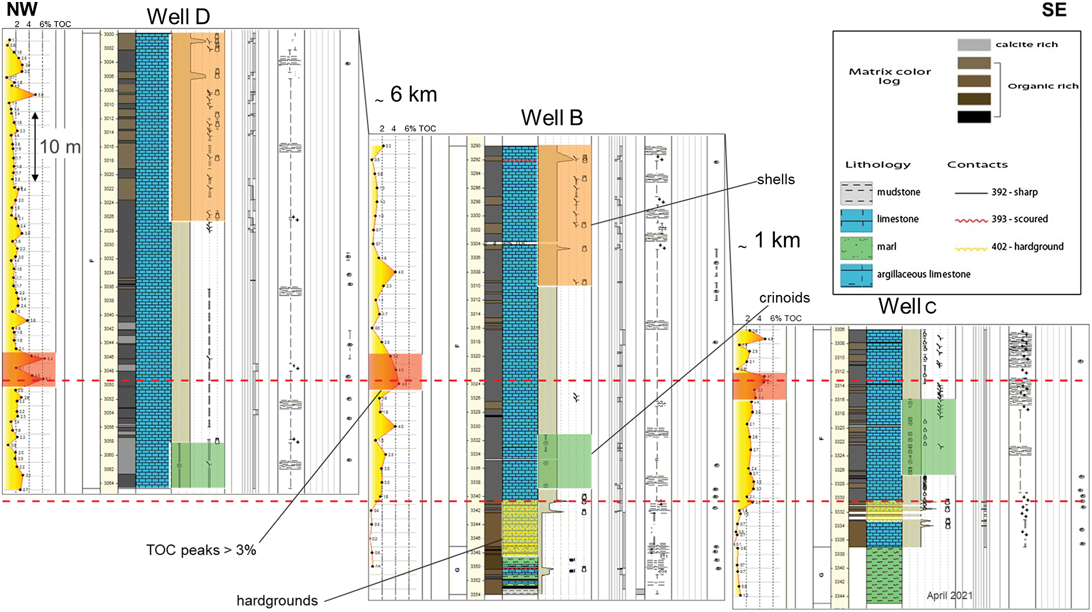
Fig. 6. Correlation panel. The uppermost red line shows a high-confidence correlation of the TOC-rich interval between the three wells. The lowermost red line illustrates the correlation of the hardgrounds at the bottom of the F member in two of the wells.

Fig. 7. (a) Hardground in light brown carbonates; the core sample is approximately 10 cm wide. (b, c) Pervasive presence of crinoids (recognized as the light-coloured particles) in Well B and Well C. The stickers indicate the depth of the core sample. Note that the bedding is oblique to the long axis of the core.

2.c.2. Total organic content analysis

TOC analyses were performed on wells B, C and D. Samples were taken at regular spacing of approximately 1 m along the cores (Fig. 6). A detailed view of the TOC content in Well C is shown in Figure 8a.

Fig. 8. (a) Illustration of the correlation between TOC values (yellow) with the global GR log (red) and the spectral GR uranium log (blue). (b) Schematic representation of the layer-cake configuration of the Abu Roash F. (c) The organic-rich layer is laterally extensive (more than 6 km), as suggested by spectral GR uranium data.

An organic-rich interval with TOC values generally above 4% can be identified in the three cores at a similar stratigraphic depth, that is, Well B at 3322–3330 m measured depth (MD), Well C at 3307–3314 m MD and Well D at 3046–3050 m MD (Fig. 6).

2.c.3. Well correlation

The correlation of the high-TOC interval suggests that the development of organic-rich layers was widespread between wells B, C and D following a layer-cake configuration. In each core, this high-TOC interval can be linked to a positive response of the spectral gamma-ray (GR) and, especially, its uranium component (GR; Fig. 8a). However, isolated high-TOC peaks are not visible in the GR uranium log (Fig. 8a), which seems to record a positive signal only when the organic-rich interval is persistent for more than 2–3 m.

The TOC variations cannot be directly correlated with the colour of the core. Although high-TOC layers are predominantly observed in dark-coloured intervals, the dark intervals do not always show high-TOC value. This implies that the TOC measurements remain essential to characterize the organic content of the cores. Nevertheless, the colour of the core is of high interest because it shows a strong link to the mechanical stratigraphy. Dark intervals more frequently exhibit fewer fractures than light intervals. The colour of the core was therefore chosen as one of the important factors for the fracture characterization and modelling in the following sections. Based on the sedimentological, TOC and spectral GR log observations, our base-case conceptual depositional scenario is a layer-cake configuration of the Abu Roash F Member over a distance of at least 6 km (Fig. 8).

2.d.1. Core observations

Detailed fracture observations have been made of the vertical and horizontal cores. It is important to note that the presence of horizontal cores is rather exceptional. The core observations were systematically compared with the corresponding BHI to check and calibrate the BHI fracture interpretations, particularly important in discriminating between natural and induced fractures. These observations were aimed at identifying and classifying different fracture types to help define scenarios of fracture connectivity and their importance on sweep, and isolate which fractures should be captured in the fracture models. The cores exhibit both natural and induced fractures. Natural fractures formed at depth due to the deformation of rock units under various tectonic stress/strain and fluid pressure regimes; induced fractures are related to the failure of rock during drilling, core recovery or transport. Filtering out the induced fractures from the observations is key to constrain accurate subsurface fracture distributions. In this study, the main criteria used to identify induced fractures on cores are (i) the absence of mineralization (calcite, tar, etc.); (ii) whether geometry is parallel or sub-parallel to easy cleavage planes (e.g. bedding surfaces; Fig. 9a, b); (iii) the presence of fractographic features (e.g. radial plumose and/or concentric arrest lines; Fig. 9a–c) with clear evidence for propagation of the fracture front towards the edges of the core (Fig. 9c); (iv) fracture initiation at sedimentary defects or at impact points (Fig. 9c); and (v) the presence of shortcuts (i.e. small rupture planes) reaching the core edge (Fig. 9c).

Fig. 9. Recognition criteria of natural and induced fractures. (a) Photograph and (b) interpretation of an induced fracture parallel to bedding. The recognition criteria are (1) main initiation point (ammonite), (2) plumose features with radial geometry, (3) arrest lines and (4) secondary initiation point (matrix heterogeneities). (c) Picture of an induced fracture and some of its recognition criteria. (d–f) Example of a natural fracture and its recognition criteria (presence of tar and mineralization). (d) Core photograph, (e) core interpretation and (f) geological interpretation of the core sample in a greater context. (g, h) Examples of mineralized natural fractures perpendicular to bedding.

The main criteria used to identify natural fractures on cores are (i) the presence of internal mineralization (e.g. calcite, pyrite; Fig. 9g, h); (ii) the presence of tar (Fig. 9d, e); (iii) being distributed in well-constrained orientation sets; and (iv) often being orthogonal or strongly oblique to bedding planes.

A fracture typology (fracture Type I, II and III) has been defined using core observations based on their morphologic expression on core (e.g. whether cutting the entire core, whether clustered, whether creating severe core degradation), their relationship to the matrix (mechanical stratigraphy), their aperture and their expected impact on flow in the subsurface.

Type III fractures (Fig. 10a, b) represent the smallest-scale fractures. They show hairline geometry and partial to total calcite cementation. Macroscopically, Type III fractures can be defined as veins, which are essentially characterized by relatively small height (or length) to aperture ratios. In the observed cores, the typical apparent height of Type III fractures varies from a few centimetres to a few tens of centimetres, while the apparent (cemented) aperture varies from a few tens of microns to 1 mm. They stop at minor sedimentary interfaces, are rarely visible on all core sides and rarely correlate with BHI observations. They are locally connected to Type II or to other Type III features. Individually or cumulatively, they provide limited storage volume. When open or partially open, they potentially form minor local flow paths when organized in small clusters of limited vertical extent (see online Supplementary Fig. S2).

Fig. 10. Core picture and interpretation of Type III, II and I fractures. (a, b) Type III fracture. Note that the fracture plane ends within the darker matrix. (c, d) Type II fracture. The black shiny material on the core is tar. (e, f) Type I fracture which corresponds to a cluster of Type II fractures. The black shinny material on the core is tar.

Type II fractures (Fig. 10c, d) represent intermediate-scale fractures. The fracture trace cuts all the visible core circumference and often bedding planes. The fracture surface is generally rectilinear. They are often open on most of the observed section. In most cases, they show a fine layer of sparitic cement on the fracture plane and are often filled with oil or tar. They occasionally appear to correlate with BHI features, but correlations are tentative because of the overall poor image quality (see the following section on BHI calibration). They are expected to provide storage volume and flow paths at well scale, especially when organized in small clusters (e.g. relatively small spacing but with limited vertical extent; see online Supplementary Fig. S3) not large enough to form Type I fractures.

Type I fractures (Fig. 10e, f) represent the largest features. They correspond to fracture zones recognized as dense clusters of smaller-scales fractures (Types II and III). They occasionally correspond to fracture corridors (Olson, Reference Olson, Cosgrove and Engelder2004; Bazalgette et al. Reference Bazalgette, Petit, Amrhar and Ouanaïmi2010; Lamarche & Gauthier, Reference Lamarche and Gauthier2018; de Joussineau & Petit, Reference de Joussineau and Petit2021; Viseur et al. Reference Viseur, Lamarche, Akriche, Chatelée, Mombo Mouketo and Gauthier2021; JP Petit, pers. comm., 2022) and possible fault zones. They are difficult to observe in detail on core because of poor recovery, and poor core recovery has become a potential recognition criteria of the presence of a Type I fracture. They are potentially visible on BHI as high-conductivity zones, and individual fracture planes and fault planes may be identifiable (see following section on BHI calibration). They are expected to play a role as major drains at reservoir scale and are essential to capture for the dynamic flow simulation.

Figure 11 illustrates the outcrop expression of Types I and II fractures to help visualize how the limited core observations could be extrapolated away from the wells. Mechanically layered sequences cropping out in Wadi Digla (near to Abu Roash village), composed of alternating carbonate-rich and argillaceous-rich units, have been interpreted as an analogue of the subsurface Abu Roash F. Type I fractures correspond to clusters associated with small-scale fault damage zones. These fractures can be classified as non-stratabound fractures following the nomenclature used by Odling et al. (Reference Odling, Gillespie, Bourgine, Castaing, Chiles, Christensen and Fillion1999) or Panza et al. (Reference Panza, Agosta, Zambrano, Tondi, Prosser, Giorgioni and Janiseck2015). They also follow the criteria used to describe highly persistent fractures (HPF) in Bazalgette (Reference Bazalgette2004) and Torrieri et al. (Reference Torrieri, Volery, Bazalgette and Strauss2021). They create potentially extensive vertical connections in the cliff section and form highly fluid conductive features in the subsurface. Type II fractures have a more limited vertical extent controlled by individual mechanical units (typically one or a few beds). They can be classified as stratabound (Odling et al. Reference Odling, Gillespie, Bourgine, Castaing, Chiles, Christensen and Fillion1999; Panza et al. Reference Panza, Agosta, Zambrano, Tondi, Prosser, Giorgioni and Janiseck2015) or as bed-controlled fractures (BCF) and multiple bed fractures (MBF) following Bazalgette (Reference Bazalgette2004) and Torrieri et al. (Reference Torrieri, Volery, Bazalgette and Strauss2021).

Fig. 11. Outcrop expression of Type I and II fractures: (a, b) photograph and (c, d) semi-interpretative drawing. (a, c) Type I fracture zone associated with small-scale fault damage zones (Wadi Digla, Egypt). (b, d) Type II fractures concentrated in stiff carbonate mechanical units (near Abu Roash village, Egypt).

An attempt was made to characterize the fracture connectivity at core scale. Observations made on both horizontal and pilot cores show several natural fracture sets. Based on observations of fracture Types II and III, fracture orientations could only be approximately derived on the few metres of horizontal cores that could be oriented. However, the time frame of the study did not allow us to include detailed fracture logging in the cores or BHI. Nevertheless, two orientation sets are clearly sampled along the available horizontal cores. The densest set is oriented NW–SE (parallel to the palaeo- and present-day maximum horizontal stress direction); a second set with a N–S orientation is observed. Other fracture orientations (NE–SW, E–W) are found locally but with much wider distributions. The different sets frequently interact, showing clear cross-cutting relationships. Figure 12 shows an example with five fractures (three Type II and two Type III). Two Type II fractures intersect physically within the core while the third Type II fracture is inferred to cross-cut the two cross-cutting Type II fractures by extrapolating the fracture plane outside of the core. Note that the Type III fractures stop at bedding interfaces. Two more examples are documented in online Supplementary Figures S4 and S5. These observations demonstrate that Type II fractures have the potential to create a connected network provided that the effective aperture of the different sets is sufficient in subsurface conditions. Samples were selected for thin-section analysis to provide an estimate of the aperture range of Type III fractures, described below (Section 2.d.3) after the calibration with the BHI data.

Fig. 12. Orthogonal Type II and III fractures and re-opened bedding. (a) Core photograph; (b) semi-interpretative drawing; and (c) fracture type and bedding interpretation.

2.d.2. Borehole image observations

BHI-based fracture interpretations were carried out for vertical and horizontal wells. Systematic comparisons with the core observations have been made, aiming to validate and calibrate the BHI results. The quality of the BHI data varies with regards to the well type. The borehole images from pilot sub-vertical wells provide a reasonably good-quality micro-resistivity image (OMRI, San Martin et al. Reference San Martin, Kainer, Elliott, Pittar, Schaecher, Morys, Goodman, Kusmer, Davies and Buchanan2008) despite the use of OBMI (Oil-Base Micro Imager). Although this qualification is subjective, the images were of sufficient quality to enable the interpretation of features that could be correlated with features observed on cores. The imaging in the horizontal sidetrack well is of poorer quality because of the often extremely dense networks of induced fractures. Notwithstanding the generally poorer image in the horizontal well, we were able to calibrate the core/log shift using wireline logs and core GR. However, some uncertainty remains about the positioning of the core along the trajectory of the different cored sections. This point has to be kept in mind with respect to the confidence placed in the following observations.

Figure 13 illustrates examples of Types I and II fractures observed on cores compared with their BHI signature. Figure 13a shows the signature of a Type I fracture zone. Three conductive fractures in the BHI have been identified and interpreted to correlate with a zone of poor core recovery (rubble zone). The sigmoidal dashed grey line in Figure 13a highlights the observations from some of the pads used to interpret one fracture plane. It is not possible to observe the segments in the BHI from the other fractures. The picture of the BHI displayed is a compressed image created with a 1:20 horizontal to vertical ratio, while the interpretation has been carried out at an uncompressed scale between 1:1 and 1:5 (Serra, Reference Serra1989). This explains why the other two fractures interpreted are not observable on the figure. Figure 13b shows the example of a Type II fracture clearly visible on core, but not visible on the BHI. An example of a small-scale fault recognizable on the core due to the presence of slickensides with fine calcite gouge, visible on the BHI as a continuous sinusoid, is illustrated in online Supplementary Figure S6. None of the Type III small-scale fractures identifiable on cores are visible on the BHI because they are to small and beyond the resolution of the BHI images.

Fig. 13. (a) BHI and core expression of a Type I fracture zone. The BHI (OMRI enhanced, OBMI dynamic) shows a highly conductive interval (darker colour). The sigmoidal shape outlined with a dashed grey line highlights the sinusoid segments that have been used to interpret one fracture plane. (b) Example of a Type II fracture clearly visible on core, but not visible on the BHI.

Figure 14 is an example of core and BHI interpretation along the horizontal well. In total, 16 natural fractures are visible on the core while 24 fractures have been interpreted on the BHI. Among the 16 natural fractures visible on the core, only four fractures could be confidently matched with fractures on the BHI. These are indicated by the dark blue arrows. The fractures indicated by the light blue arrows do not match the BHI interpretation. Twenty of the fractures interpreted on the BHI do not correspond to any fractures on the core; these are indicated by the red arrows. These features, which are systematically aligned with the direction of the present-day in situ stress, are interpreted as drilling-induced fractures.

Fig. 14. Discrepancy between fracture observed on core and on BHI, acquired while drilling along horizontal wells. The natural fractures interpreted on the core are indicated by the arrows at the top of the picture, while the fractures interpreted on the BHI are indicated by the arrows at the bottom of the picture. The numerous induced fractures hinder the interpretation of the natural fractures. They are aligned with the present-day maximum horizontal stress direction.

2.d.3. Thin-section observations

Core observations are obviously not adequate to estimate the internal aperture of Type I and II fractures because of the significant change in stress state from downhole to the surface; any information about their true subsurface aperture is lost. Type III fractures consistently show a pervasive calcite cementation, which usually ensures good recovery and preservation of the cored sections that contain Type III fractures. Under the hand-lens, at least in some of these Type III fractures, open space was locally observed within their calcite cemented volume (Fig. 15). The presence of a remaining aperture within the fracture partially filled with organic content is limited to one clear example on thin-section (Fig. 15b, c). This suggests that the contribution of Type III fractures to the Abu Roash F storage capacity and to its permeability may be considered as negligible or at least extremely limited.

Fig. 15. (a) Sketch based on Type III fractures observed on the AR-F cores. The fracture shows calcite cementation but preserves a small and irregular remaining internal aperture: (1) fracture walls, (2) calcite cementation, (3) preserved aperture and (4) local calcite bridging. This sketch is based on hand lens observations of Type III fractures observed on cores. (b) Photo-micrograph of a Type III fracture with evidence of remaining apertures filled with organic matter (kerogen or bitumen). (c) Semi-interpretative drawing.

The timing of the fracture formation and the evolution of fracturing episodes have been interpreted from the morphology of the fractures observed on thin-sections cut in a plane approximately perpendicular to bedding. The traces of Type III fractures are usually sinuous and even often folded (Fig. 16). This implies that such fractures have been submitted to a layer-orthogonal shortening after and/or during their propagation (Pollard & Aydin, Reference Pollard and Aydin1988). Such shortening occurs when fractures initiate before the rock is fully compacted, and implies that the sediments became brittle at a relatively early post-depositional timing (Eberli et al. Reference Eberli, Baechle, Anselmetti and Incze2003; Lamarche et al. Reference Lamarche, Lavenu, Gauthier, Guglielmi and Jayet2012; Lavenu et al. Reference Lavenu, Lamarche, Salardon, Gallois, Marié and Gauthier2014). In very deformed cases (Fig. 16a, b), the development of the fracture visibly continued during the compaction-related folding and caused the formation of secondary fracture branches, which show a lower amplitude of folding. While stylolites are hardly visible at the scale of the core, thin-sections reveal a high density of them (as well as smaller-scale and smaller-amplitude pressure/solution seams). These features are distributed along bedding-parallel planes. The high density of stylolites and solution seams suggests that pressure solution mechanisms have potentially accommodated a large part of the total compaction and volume loss.

Fig. 16. (a, b) Thin-section showing a syn-compactional Type III fracture. (a) Photomicrograph and (b) semi-interpretative drawing; (1) stylolites and/or pressure solution seams, locally deformed; (2) elongated, calcite-rich bioclasts with evidence of compaction-related strain; (3) folded Type III fracture with cement dominated by blocky ferroan calcite crystals (in pink/purple); (4) secondary cement (blocky calcite showing lower iron content, and little remaining open void (in black); (5) secondary fracture showing lower amplitude of syn-compaction folding; (6) matrix fragments included within the calcite cement (evidence of crack-seal mechanisms); and (7) deformed cement (micro-breccia) in the folded fracture. (c, d) Thin-section showing a syn-compactional Type III fracture. (c) Photomicrograph and (d) semi- interpretative drawing: (1) Type III fracture with blocky ferroan calcite cement; (2) stylolite cross-cutting the fracture (clearly post-dating the fracture development); identified from the content of opaque material (interpreted as organic matter); (3) fragments of matrix included in the blocky calcite cement; and (4) deformed cement (micro-breccia) essentially distributed at the immediate neighbourhood of the stylolite plane.

Figure 16c and d illustrate that such stylolites are also commonly deformed by further compaction processes (see online Supplementary Figs S7 and S8 for higher-resolution versions). Deformed carbonate clasts (4 in Fig. 16b) also illustrate the effect of such compaction. In parallel, the calcite cement of Type III fractures is also sometimes clearly dissolved by pressure solution at stylolite surfaces (Fig. 16c, d). These combined observations imply that the initiation of pressure solution and of the folded Type III fractures may have occurred almost simultaneously, or that these two processes were, at least, acting simultaneously at one point in the deformation history. However, it is possible that the pressure solution processes (stylolite formation) may have initiated slightly before the onset of fracturing. Observations often indicate that very localized fluid over-pressure can generate during stylolitization and may locally trigger the initiation of veins and other small fractures orthogonal to bedding and bed-parallel stylolites (Engelder, Reference Engelder1987; Pollard & Aydin, Reference Pollard and Aydin1988). This process is particularly relevant at a scale representative of Type III fractures.

Detailed observations of the fracture infilling commonly show several stages of calcite cementation (blocky calcite texture), which tend to form layers of crystals subparallel to the fracture walls. The fracture volume also contains numerous fragments of matrix that are included in the cement (Fig. 16a–d). These observations suggest that the propagation and opening of Type III fractures occurred in several stages, and involved crack-seal mechanisms (Ramsay, Reference Ramsay1980) that can explain the presence of matrix fragments within the fracture cement. The intra-fracture calcite cement is itself very often deformed and locally presents a micro-breccia texture. This texture tends to localize in the zones where the fracture is most deformed. They correspond especially to zones of intense folding (Fig. 16b-7) and zones localized in the immediate neighbourhood of some post-fracturing stylolites (Figure 16d-4). More rarely, other minerals such as barite (see online Supplementary Fig. S9) and traces of organic matter (kerogen or bitumen; Fig. 15b, c) can be distinguished. In summary, regarding the cementation history, and assuming that the early to syn-compaction origin of Type III fractures is correct, the observations and interpretations discussed above imply that the fracture cement was crystallized before compaction was completed. In this interpretation scenario, fractures were cemented very soon after they were created. This may explain the fact that the most deformed (folded) Type III fractures, which should also be the earliest, show very little evidence of remaining void. The observations and interpretations listed in the previous paragraphs suggest an early (syn- compaction) origin for the Type III fractures.

Figure 17 proposes a simplified kinematic scenario to illustrate the initiation and the evolution of a Type III fracture during the compaction of the AR-F formation, based on Figure 16a–d. The following chronology of deformation/fracturing is proposed based on the observations described in the paragraphs above: (1) onset of compaction; (2) onset of bed-parallel pressure solution and stylolitization; (3) initiation of Type III fracturing (simultaneous cementation); stylolitization continues; (4) syn-compaction deformation (folding) of Type III fracture; (5) end of major compaction; and (6) onset of larger-scale fracturing (not represented in Fig. 17). The data did not allow discrimination between the chronology of Type I and II fractures.

Fig. 17. Simplified kinematic scenario (vertical section views) to describe the initiation and evolution of a Type III fracture, based on the previously described examples (note that the different colours represent successive stages of cementation): (a) fracture initiation during compaction-associated stylolitization; (b) fracture propagation and aperture increase with crack-seal mechanism, onset of fracture folding due to compaction; (c) amplification of syn-compaction fracture folding; the folding of the fracture plane(s) involve the onset of slight shear movement and the creation of small extensional jog between two fracture segments; (d) the folding of the fracture is associated with the deformation of the surrounding bedding and triggers the rotation of the zone that contains the small extensional jog while it is cemented with calcite; (e) deformation amplifies following the kinematics described in (c) and (d) and results in a structure based on Figure 16. Note the increasing number of pressure/solution features (in black) from (a) to (e).

2.d.4. Mechanical stratigraphy observations

The final part of the characterization is to examine considerations specific to mechanical stratigraphy. In many cases, vertical and lateral variation of argillaceous content and/or porosity have a large impact on the mechanical behaviour of sedimentary rocks and, therefore, fracture development. The observations made on the available cores tend to show that (i) the argillaceous content is negligible; and (ii) matrix porosity does not vary significantly laterally within the formation. As a result, no obvious or quantifiable relation between these parameters and the fracture intensity could be observed. Conversely, a qualitative, visual correlation appears to exist between fracture intensity, particularly of the Type III fractures, and matrix colour. This colour is weakly linked to the organic matter content as mentioned above in the reservoir architecture section. The local organic content seems to counteract the effect of the carbonate content. It is expected to have a strong impact on the stiffness and brittleness of the rock, especially at the onset of fracturing during the early stage of burial (Afşar et al. Reference Afşar, Westphal and Philipp2014; Lavenu & Lamarche Reference Lavenu and Lamarche2018). The distribution of light- and dark-coloured layers is documented in Figure 18 based on the sedimentary analysis from core observations. A tendency for more and thicker dark-coloured layers towards the bottom of the core than at the top is observed (Fig. 18a).

Fig. 18. Qualitative links between matrix colour and fracture intensity. (a) Sedimentary logs for one vertical pilot hole. Note the increase of dark-coloured matrix towards the bottom of the cored section. (b) Comparison with the fracture intensity log (unoriented fracture picks on acetate sleeves) shows that the highest fracture intensity tends to correlate with the units that show a lighter matrix colour.

A relationship between the location of light-coloured (carbonate-rich) intervals and the frequency of fractures has been observed. This tendency has been visually identified by direct observations on cores and validated by comparison with a fracture intensity log computed from the fractures picked on acetate sleeves (Fig. 18b). A clear impedance effect of interfaces between dark- and light-coloured layers on the propagation of Type III fractures has also been observed. Fractures generated in light-coloured units tend very often to stop or to die-out at the transition with dark-coloured units (Fig. 19). Observations along horizontal cores (Fig. 19) in which boundaries between lighter- and darker-coloured matrix have been sampled are a powerful demonstration of the impact of mechanical stratigraphy.

Fig. 19. Example of core-scale mechanostratigraphic control of light- versus dark-coloured units on the distribution and propagation of Type III fractures. (a) Photograph of horizontal core showing a Type III fracture interacting with light-/dark-coloured bed interface. (b) Interpretive picture showing that the fracture cross-cuts the entire visible light-coloured interval and progressively dies out after passing the interface with the dark-coloured interval.

The control of dark- versus light-coloured unit alternations on the propagation of Type III fractures has also been observed in a single partial thin-section (see online Supplementary Fig. S10). Although part of the matrix is missing on one side of the fracture, it is possible to observe a morphological change occurring in a zone where a Type III fracture cuts through a dark- and light-coloured matrix interface. The Type III fracture observed here shows an apparent cemented aperture of c. 200 µm and presents a rather regular geometry in the calcite-rich unit. It becomes thinner (with apparent cemented aperture of c. 25–50 µm), shows a hairline geometry with a tendency to anastomize, and then quickly dies out within the dark unit.

2.e.1. Conceptual fracture diagram

The first step of the fracture modelling is to draw a conceptual geological diagram capturing the key observations and the overall understanding of the fracture network. This does not necessarily need to be a sophisticated digital diagram elaborated using a drawing package nor a piece of art. Independent of the competence of the geoscientist to draw, it is fundamental to represent the concept on paper first before moving to the 3D fracture model proper. The hand-drawn illustration in Figure 20a summarizes the key observations from cores and places them in a structural context, considering information from the regional context and the seismic data. The vertical pilot well (D in Fig. 5c) with the largest number of Type I fractures is located in the hanging wall of a large transtensional fault. The horizontal appraisal well (D in Fig. 5c) and the other vertical pilot (B in Fig. 5c), with a much smaller number of Type I fractures, are located in a less-deformed area, at a larger distance from seismically imaged faults.

Fig. 20. (a) Preliminary sketch of the conceptual fracture diagram showing the position of pilot wells and horizontal side-track in a block diagram including Type I fault-associated fracture zones and Type II fractures. The Type III fractures are not represented on this simplified block diagram. (b) Conceptual 3D diagram summarizing the spatial distribution of Type I fault-associated fractures. The structural style of the diagram is based on the Top Abu Roash Depth map shown in Figure 5, as well as the transtensional structural setting.

This preliminary diagram is a useful vehicle to expose our understanding of the fracture network geometry based on our observations, after the core visit with the project team. The most important features that need to be captured in the fracture models are the faults and their associated fault damage zones that create the largest fluid conduits in the subsurface. The initial diagram can then be turned into a more sophisticated 3D conceptual block diagram summarizing the spatial distribution of Type I fracture zones in a setting inspired from the Abu Roash F seismic-scale structural setting (Fig. 20b). Note that in this diagram, wells A and B are in communication through the connected damage zones of small-scale faults. Conversely, Well C is located within the damage zone of a larger fault but does not show any connection to wells A and B. Well D also penetrates a major fault. Note that wells C and D are located in areas expected to be most deformed given their proximity to large, seismic-scale fault zones. Tar is present in these wells (C and D), interpreted as an indication of fluid migration along these faults. We decided to capture these faults explicitly in the fracture model and use the seismic data (see following section) to constrain their location, as they are most important features for dynamic simulation.

2.e.2. Input from seismic data

The seismic dataset available for this work included a seismic cube in time format with various seismic attributes (e.g. semblance, dip-azimuth, dip), a time and depth-converted Top Abu Roash F horizon and a set of coarse fault polygons. The initial coarse fault polygons were calibrated against the seismic data to assess whether additional faults (mapped as single lineaments on horizon surfaces rather than mapped as 3D fault surfaces) could be considered as input to the fracture modelling. A small-scale multidirectional horizon curvature attribute (Lisle, Reference Lisle1994; Roberts, Reference Roberts2001; Hart et al. Reference Hart, Pearson and Rawling2002; Srivastava & Lisle, Reference Srivastava and Lisle2004; Lisle & Toimil, Reference Lisle and Toimil2007; Lisle et al. Reference Lisle, Toimil, Aller, Bobillo-Ares and Bastida2010), with a 100 m wavelength, has been computed for the Top Abu Roash F time horizon to help highlight potential faults from the geometry of the horizon that had not been explicitly mapped on the 3D data (Fig. 21a). This has been compared with a sharp semblance attribute painted at Top AR-F (Fig. 21b) to confirm the consistency between the two sources of data. The initial fault polygons of a coarse, large-scale interpretation have been compared with the small-scale curvature attribute (Fig. 21c) and the seismic semblance. Note that these initial fault polygons match only the largest-scale features highlighted by the horizon curvature. Smaller-scale faults (with lower throw) were subsequently mapped based on the multidirectional horizon curvature and semblance attributes. These are displayed in Figure 21d and have been used as input to the DFN model elaboration.

Fig. 21. Top Abu Roash-F fault interpretation. (a) Small-scale (100 m) wavelength multidirectional horizon curvature computed for Top Abu Roash F time horizon. (b) Sharp semblance attribute painted on time horizon. (c) Comparison of the initial coarse fault polygon model with small-scale wavelength multidirectional horizon curvature attribute. (d) Updated fault model from manual picking based on the multidirectional horizon curvature and seismic attributes.

2.e.3. Mechanical stratigraphy concept from core observations

From the core observations, it is possible to propose several high-level mechanical stratigraphy rules to be considered for input to the fracture modelling. For Type I fracture zones, the fault damage zone is more intensely fractured in the calcite-rich units than in the organic-rich units, with high vertical continuity immediately adjacent to the fault and vertical continuity limited by organic layers identified in the cores and transferred to the model. Type II fractures are common in the carbonate-rich units and rare in high-TOC units. The vertical continuity may be limited by interfaces with the highest contrast between light- and dark-coloured (carbonate-rich/organic rich) units. Type II fractures are denser in light-coloured (carbonate-rich) units. These rules can be used in combination with 3D grids of matrix properties to either constrain the creation of discrete fracture objects from seeds or create directly and implicitly fracture properties in grid cells (i.e. straight-to-cell approach; Rawnsley et al. Reference Rawnsley, Swaby, Bettembourg, Dhahab, Hillgartner, de Keijzer, Richard, Schoepfer, Stephenson and Wei2004; Richard et al. Reference Richard, Rawnsley, Swaby and Richard2006). However, the complexity of the approach as well as the accuracy of the result achieved needs to be balanced against the actual data used to calibrate the final model results.

2.e.4. Results of discrete fracture network models

Two sets of fracture models have been created. The first set consists of simplified 3D box-shaped grids (Fig. 22) around key wells. In these models, the fractures are taken into account as continuous properties in simulation grids. These models were designed with homogeneous (fractured) volumes (Fig. 22a, b) or with an interface between two main units with contrasting fracture intensities (Fig. 22c, d). The presence of a high-permeability conduit, which mimics the effect of an intensely fractured fault damage zone, was also introduced (Fig. 22b, d). These models are particularly useful to test sensitivity analysis of fracture parameters.

Fig. 22. Box model configuration to test fracture parameters around key wells. The dimensions vary between 500 m and 1 km. Homogeneous matrix and fracture properties are applied. The orange polygon represents a fault damage zone.

The second set of models portray the realization of DFNs in 3D grids. Figure 23 illustrates several potential scenarios with varying complexity to capture the mechanical stratigraphy and its impact on fracture distribution. In scenario 1 (Fig. 23a), discrete fractures are modelled in the damage zones of faults. Their vertical distribution is homogeneous within the different layers of the model. Scenario 2 (Fig. 23b) is relatively coarse and simplified in an attempt to portray the mechanical stratigraphy of the formation. The Abu Roash F is divided into two different groups of layers (upper and lower units). The upper unit (three layers in the model) is considered more brittle and contains a high fracture intensity. Conversely, the lower unit (three layers in the model) is modelled with fewer fractures due to a higher organic content overall. Scenario 3 (Fig. 23c) includes a slightly more complex distribution of the units, representing the mechanical stratigraphy. Brittle (light-coloured, carbonate-rich) units are modelled with alternations of more plastic (dark-coloured) units in which fracture intensity is expected to be lower. Finally, Scenario 4 (Fig. 23d) represents the realization of a detailed sector model, including Type II fractures of small dimensions around key wells. Scenarios 1 and 2 have been implemented in the discrete fracture network models illustrated in Figure 24a, and in Figure 24b and c, respectively. Scenarios 3 and 4 are intended to examine the impact of fracture network geometry on production and help the validation and calibration of fracture properties at smaller scale once dynamic data become available. Scenario 4, which is the most detailed, would also have great value during discussions with other disciplines when planning in-fill wells (Richard et al. Reference Richard, Pattnaik, Al Ajmi, Kidambi, Narhari, Le Varlet, Guit and Dashti2015). This scale of model has not been built as part of this study.

Fig. 23. Mechanical layer scenarios for the DFN models.

The key constraint for the fracture models is the established dynamic connection between wells A and B. Pressure depletion, due to early production from Well A, was observed in Well B at the time of drilling. Based on the tight permeability of the matrix and the production data from Well A, the productivity from the fracture component has been assessed and confirmed. Different cases of discrete fracture networks were designed on the basis of (i) the fault model used to constrain the Type 1 fractures (initial coarse model or refined lineaments); (ii) the scenarios of mechanical-stratigraphy (homogeneous, two-layer or multi-layered; Fig. 23) and the fault damage zone width. These cases only included Type I fracture zones. The DFN models were built using SVS Fault and Fracture Solutions software (Rawnsley et al. Reference Rawnsley, Swaby, Bettembourg, Dhahab, Hillgartner, de Keijzer, Richard, Schoepfer, Stephenson and Wei2004; Richard et al. Reference Richard, Lamine, Pattnaik, Al Ajmi, Kidambi, Narhari, Le Varlet, Swaby and Dashti2017). The DFN fracture objects have a rectangular geometry and fit within the grid layers. Their distribution and geometrical attributes are controlled by 3D grid properties. After the creation of the different DFN models, 3D arrays of fracture properties (e.g. permeability, spacing, shape factor, porosity) were generated for the dynamic flow simulation. We present the results of three different DFN model realizations referred to as Cases 1, 2 and 3.

The first static model built for Case 1 DFN was built using a grid cell size of 100 m × 100 m. The faults used in the model correspond to the initial coarse fault interpretation. In this first-pass model, the grid orientation was arbitrary and does not align with the main fault and fracture orientations. A detailed, large-scale view of our Case 1 DFN model is depicted in Figure 24a (an overall view and higher-resolution versions are available in online Supplementary Figs S11–S14). A relatively large width of fault damage zones of 200 m was imposed in the model. The width of the fault damage zone is driven by the 3D grid cell size. Despite the large cell size used for the simulation grid and the large width of the modelled fault damage zones, the model failed to give a satisfactory history match of the production data because of the lack of connectivity between well A and B. While Well A appears to be cutting through an intensely fractured zone localized at the intersection between two faults (Fig. 24a), wells B Pilot and B Horizontal are visibly not connected to any intensely fractured cells. This connectivity mismatch is simply the result of the fault model used for this realization. The initial coarse interpretation is not detailed enough. The fracture model misses smaller-scale faults and their related fault damage zones, which can ensure dynamic communication between the wells.

Fig. 24. Detailed view of the DFN models and grid cells with high fracture intensity representing the fault damage zones. The warmer and colder colours represent higher and lower fracture intensity, respectively. (a) Case 1 DFN. The cells size is 100 m × 100 m. Because of the absence of faults close to Well B trajectories, wells B Pilot and Horizontal (hz) are not dynamically connected to Well A via fault damage zones. (b) Case 2 DFN. The cells size is 25 m by 25 m. Wells B Pilot and Horizontal (hz) are cutting through the damage zones of two fault segments which are connected through a relay zone. However, Well A is not connected to the fault damage zone. (c) Case 3 DFN. The cells size is 25 m by 25 m. In this realization Well A is connected to wells B Pilot and B Horizontal (hz) via the 50 m wide fault damage zones. Wider views of the DFN are available in online Supplementary Figs S11–S14.

The Case 2 DFN model was generated in a 3D grid built using a grid cell size of 25 m × 25 m together with the faults from a refined fault interpretation. The model therefore has many more faults than the Case 1 model (see Fig. 21 for a comparison of the coarse and refined fault lineaments). The grid was oriented such that it aligned with the main fault and fracture orientations. A 50 m wide fault damage, corresponding to one grid cell on either side of the modelled faults, was used to build the DFN. A detailed view, centred on wells A and B of the Case 2 model is shown in Figure 24b. Because of the presence of the additional faults compared with Case 1, Wells B Pilot and B Horizontal are now connected to a zone of intense fracturing, specifically through a fault relay. However, in this realization, Well A is not connected to the nearby fault damage zone because of the narrower modelled fault damage zone (2 × 25 m) compared with Case 1 and the new grid orientation. As a result, as in Case 1, the model failed to give a satisfactory history match with the production data because the dynamic connection between wells A and B is not honoured. An alternative and complimentary explanation may also be linked to the relative inaccuracy of the fault model used to constrain the fracture distribution.

Our Case 3 fracture model was built in the same grid as Case 2, with a 25 m × 25 m cell size. The faults used in the model correspond to the refined fault interpretation. The key difference from the Case 2 model is the width of the fault damage zones, now 50 m on each side of the fault surface. This corresponds to two grid cells on either side of the modelled fault. This wider damage zone has been implemented to allow for dynamic communication between the wells. This model enables Well A to be connected to a zone of high fracture intensity. At the same time, wells B Pilot and Horizontal are also connected to the zone of high fracture intensity along the fault segment. In this realization, wells A and B are connected through the modelled fault damage zone cells across the fault relay. As a result of this connection, the model gave a satisfactory history match with the production data.