


1. Introduction
Superhydrophobic surfaces can dramatically reduce flow resistance in the manipulation of small volumes of fluid (Rothstein Reference Rothstein2010; Lee, Choi & Kim Reference Lee, Choi and Kim2016). Capillarity allows a surface microstructure to support interfaces or menisci that prevent fluid from fully penetrating interstitial regions between pillars, posts or gratings, leading to trapped gas pockets and enhanced slip over the spanning menisci. Maintaining and controlling this so-called Cassie state remains a key challenge for the successful deployment of superhydrophobic surfaces in applications (Lee et al. Reference Lee, Choi and Kim2016). There has been significant progress in improving the robustness of the Cassie state, including use of textured groove sidewalls and re-entrant, and doubly re-entrant, pillar designs (Ahuja et al. Reference Ahuja, Taylor, Lifton, Sidorenko, Salamon, Lobaton, Kolodner and Krupenkin2008; Tuteja et al. Reference Tuteja, Choi, Mabry, McKinley and Cohen2008; Lee & Kim Reference Lee and Kim2009; Hensel et al. Reference Hensel, Helbig, Aland, Braun, Voigt, Neinhuis and Werner2013).
In quantifying slip for internal channel flows, a touchstone article by Philip (Reference Philip1972) provides explicit solutions to several mixed boundary value problems relevant to the mixture of no-slip and no-shear surfaces that provide a good model of flow over superhydrophobic surfaces. Philip's solutions provide valuable benchmarks in the field of surface engineering and are by now well known (Lee et al. Reference Lee, Choi and Kim2016). His solutions assume flat interfaces are flush with interspersed flat no-slip surfaces, a feature shared with later studies (Lauga & Stone Reference Lauga and Stone2003). Sbragaglia & Prosperetti (Reference Sbragaglia and Prosperetti2007) examined how weak meniscus curvature affects slip by solving the relevant mixed boundary value problems. Their study was reappraised and extended by the present author (Crowdy Reference Crowdy2017), who showed that their slip length corrections can be found instead using integral identities, or ‘reciprocal theorems’, together with Philip's exact solutions for flat menisci. In practice, this meniscus curvature is caused by pressure differences between the trapped gas and the working fluid.
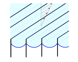
Those same pressure differences can also cause depinning of the menisci from the top of the grating, causing invasion, and partial filling, of the grooves. Figure 1(a) shows the menisci depinned from the top of the grating; figure 1(b) shows a typical re-entrant T-shaped surface design where the meniscus also partially fills the grooves (Ahuja et al. Reference Ahuja, Taylor, Lifton, Sidorenko, Salamon, Lobaton, Kolodner and Krupenkin2008; Tuteja et al. Reference Tuteja, Choi, Mabry, McKinley and Cohen2008; Lee & Kim Reference Lee and Kim2009; Hensel et al. Reference Hensel, Helbig, Aland, Braun, Voigt, Neinhuis and Werner2013). Concerning quantification of slip, there is no difference between these two scenarios (the fluid cannot ‘see’ the shape of the walls below the meniscus), although their structural robustness can certainly be expected to differ. Lee et al. (Reference Lee, Choi and Kim2016) point out that meniscus depinning and invasion of the groove have more serious consequences for slip reduction than mere curving of the menisci without depinning (Biben & Joly Reference Biben and Joly2008). Several authors have carried out numerical studies quantifying slip for partially filled cavities (Ng & Wang Reference Ng and Wang2009; Teo & Khoo Reference Teo and Khoo2010; Ge et al. Reference Ge, Holmgren, Kronbichler, Brandt and Kreiss2018), and the author has previously given some analytical formulas quantifying slip in which a small set of parameters must be found numerically (Crowdy Reference Crowdy2011a), but the extant literature contains no explicit formulas akin to Philip's that have proven so useful in the field. The present paper contributes in this direction.

Figure 1. Two scenarios involving partially filled cavities: (a) longitudinal shear flow along a periodic grating with meniscus displacement into the cavity due to depinning from the corners; and (b) a re-entrant T-shaped grating design.
The aim here is to report analytical results associated with the problems shown in figures 2(c) and 2(d): longitudinal shear over a superhydrophobic surface made up of a  $2L$-periodic grating of infinitely thin walls where the menisci between the walls have invaded the grooves between them by a distance
  $H$ and are weakly curved, making a small angle
  $\theta$ with the
  $x$ axis. An exact solution for the axial flow field
  $w_F(x,y)$ in figure 2(c) is found here for flat menisci
  $\theta =0$, for any
  $H$ and
  $L$, and for infinitely thin walls, so that
  $c=L$, where
  $2c$ is the span of the meniscus in each period window. This new solution can be viewed as a natural mathematical continuation of that found by Philip (Reference Philip1972) for shear flow over a
  $2L$-periodic array of flat no-shear slots of width
  $2c$ between flush no-slip surfaces. Those no-slip surfaces might be the flat tops of a grating as shown in figure 2(a) and whose slip length Philip found to be
 \begin{equation} \frac{2 L }{\rm \pi} \log \sec ( {{\rm \pi} \delta_P } ), \quad \delta_P \equiv \frac{c}{2L}. \end{equation}
Figure 2. (a) Philip's longitudinal flow problem where flat menisci of width  $2c$ are flush with the tops of the sidewalls of the
  $2L$-periodic grating. (b) The singular case of Philip's problem with
  $c \to L$, where sidewalls get infinitely thin. (c) The model problem considered here: continuation beyond the singular case by downwards displacement of the flat meniscus by distance
  $H > 0$ into the cavities. (d) Partially filled cavities with weak curvature of the displaced menisci. The case of downward protrusion
  $\theta < 0$ is shown: the flat case is
  $\theta = 0$. In panels (c) and (d) the sidewalls are infinitely thin.
As  $c \to L$, as in figure 2(b), this is a singular case (Schnitzer Reference Schnitzer2016) where infinitely thin walls are spanned by flush menisci. However, one can continue the solution branch beyond this singular case by displacing the meniscus into the cavity by distance
  $H$ as in figure 2(c). The slip length (relative to the top of the grating) associated with the flow in figure 2(c) can be extracted from
  $w_F(x,y)$ and is given explicitly by
 \begin{equation} \varLambda_F = \frac{2L}{\rm \pi} \log ( 1 + \textrm{coth}({{\rm \pi}\delta}) ), \quad \delta = \frac{H}{2L}. \end{equation}
The non-dimensional parameter  $\delta$ is the cavity invasion depth-to-pitch ratio.
With the analytical solution  $w_F(x,y)$ at hand, we then follow Crowdy (Reference Crowdy2017) and use integral identities to show the modified slip length
  $\varLambda (\delta , \theta )$ for weakly curved menisci. Let
  $\theta$ be the angle of the meniscus at the triple contact point relative to the positive
  $x$ axis, with
  $\theta =0$ corresponding to a flat interface. Figure 6(d) shows downward-protruding menisci with
  $\theta <0$. Here we show that
 \begin{equation} \frac{\varLambda(\delta, \theta) }{2L} = \frac{1 }{\rm \pi} \log ( 1 + \textrm{coth}({{\rm \pi}\delta}) ) + {\theta} F(\delta) + {O}(\theta^{2}), \end{equation}
where
 \begin{equation} F(\delta) = \int_{0}^{1} u (1-u) \frac{ \cos^{2} ( {{\rm \pi} u} )}{{\textrm{sinh}^{2} ({{\rm \pi} \delta}) + \sin^{2} ({{\rm \pi} u})}}\,\textrm{d}u. \end{equation}
Since  $\theta < 0$ when meniscus deflection is downwards further into the groove, and since
  $F(\delta )$ is clearly non-negative, the second term on the right in (1.3) quantifies the slip length reduction when a meniscus that has already invaded the cavity by distance
  $H$ curves downwards while pinned at that level, as shown in figure 2(d). Equation (1.3) is the analogue of a similar formula (Sbragaglia & Prosperetti Reference Sbragaglia and Prosperetti2007; Crowdy Reference Crowdy2017) for weakly curved menisci that are flush with the flat top of the grating when flat (that is, when the menisci for Philip's solution in figure 2(a) become weakly curved). Equations (1.2)–(1.4) are valid for grating walls of zero width, but it will be shown that they provide useful upper bounds on the slip lengths for realistic gratings where the groove walls will have some thickness (usually small in practice, to maximize slip). We also argue in § 5 that, although derived for unbounded shear flow, the new explicit formulas will be useful for quantifying slip in bounded channel flows too.
2. Shear flow over blades with flat menisci invading the grooves
It is convenient to set the origin in the  $(x,y)$ plane to be at the intersection of the menisci with the walls, as shown in figure 2(b). For now, the meniscus is taken to be flat,
  $\theta =0$. Since there is no imposed pressure gradient along the grating, we must solve
 \begin{equation} \nabla^{2} w_F = 0, \quad \nabla^{2} = \frac{\partial^{2} }{\partial x^{2}} + \frac{\partial^{2}}{\partial y^{2}}, \end{equation}
for a function  $w_F(x,y)$ that is
  $2L$-periodic in
  $x$ satisfying the condition of simple shear with unit shear rate in the far field,
 \begin{equation} w_F(x,y) \to y+ \lambda_F, \quad y \to \infty, \end{equation}
and where the constant  $\lambda _F$ is the slip length we seek. If one imagines an ‘equivalent’ simple shear having the form (2.2) everywhere (that is, not just as
  $y \to \infty$), then
  $\lambda _F$ is the distance below the
  $y=0$ line where an effective no-slip condition would hold, thereby providing a measure of the slip on
  $y=0$ associated with the flow
  $w_F$. The boundary conditions are that
 \begin{equation} w_F= 0 \quad \text{on the walls} \quad\text{and}\quad \frac{\partial w_F }{\partial n } = 0 \quad \text{on the menisci}. \end{equation}
For flat menisci, the latter condition becomes  ${\partial w_F / \partial y } = 0$.
To solve this mixed boundary value problem, we let  $z=x+\textrm {i}y$ and introduce the analytic function
 \begin{equation} h(z) = \phi(x,y) + \textrm{i} w_F(x,y), \end{equation}
where  $\phi (x,y)$ is the harmonic conjugate of
  $w_F(x,y)$. Philip (Reference Philip1972) solves similar mixed boundary value problems using Schwarz–Christoffel theory; here we deploy an extension of a conformal geometric method used by the author (Crowdy Reference Crowdy2011b) to retrieve and extend Philip's solutions.
Two geometrical observations lead directly to the solution. The first is that two ‘radial slit mappings’, also used in Crowdy (Reference Crowdy2011b) and described in an appendix to that paper, given by
 \begin{align} \chi_\zeta = R(\zeta,\alpha) \equiv{-} \frac{(\zeta-\alpha) (\zeta-1/\bar{\alpha}) }{(\zeta - \bar{\alpha}) (\zeta-1/{\alpha})}, \quad \chi_\eta = R(\eta, \beta) ={-} \frac{(\eta-\beta) (\eta-1/\bar{\beta}) }{(\eta - \bar{\beta}) (\eta-1/{\beta})}, \end{align}
have the geometrical effect of transplanting an upper half disc, in this case in two parametric  $\zeta$ and
  $\eta$ planes, to the interior of a unit disc with a radial slit in the respective
  $\chi _\zeta$ and
  $\chi _\eta$ image planes. The point
  $\zeta =\alpha$ in the upper half unit
  $\zeta$ disc maps to the origin in the
  $\chi _\zeta$ plane. Figure 3 shows these mappings composed with a subsequent logarithmic transformation taking these slit unit discs to vertical semi-strips with vertical slits.

Figure 3. Conformal geometric construction of the solution (2.7). Regions corresponding under the maps are colour-coded. A radial slit map, followed by a logarithm, takes the upper half unit  $\zeta$ disc to the period window in the
  $z$ plane. A similar sequence also maps it to the correct region in the
  $h$ plane but is preceded by a Möbius mapping.
The second observation is that the Möbius mapping,
 \begin{equation} \eta = M(\zeta) \equiv{-}\textrm{i} \left [ \frac{\zeta-\textrm{i} }{\zeta + \textrm{i} } \right ], \quad \beta = M(\alpha), \end{equation}
transplants the upper half disc in the  $\zeta$ plane to the upper half disc in the
  $\eta$ plane, with
  $\zeta =\alpha$ mapping to
  $\eta =\beta$. As shown diagrammatically in figure 3, this means that we can produce an explicit mapping from the same upper half unit
  $\zeta$ disc to a period window of the fluid domain and to the corresponding region in a complex
  $h = \phi + \textrm {i} w_F$ plane:
 \begin{equation} \left. \begin{gathered} z = {\mathcal{Z}}(\zeta) ={-} \frac{\textrm{i} L }{\rm \pi} \log \chi_\zeta={-} \frac{\textrm{i} L }{\rm \pi} \log R(\zeta,\alpha), \\ h = {\mathcal{H}}(\zeta) ={-} \frac{\textrm{i} L }{\rm \pi} \log \chi_\eta={-} \frac{\textrm{i} L }{\rm \pi} \log R(\eta, \beta) ={-} \frac{\textrm{i} L }{\rm \pi} \log R(M(\zeta), \beta) . \end{gathered} \right\} \end{equation}
 The colour-coded lines in figure 3 correspond as follows: the red grating walls in the  $z$ plane correspond to the red lines in the
  $h$ plane where
  $\textrm {Im}[h] = w_F = 0$, implying that these are no-slip surfaces; the blue meniscus portions in the
  $z$ plane on which only
  $x$ varies correspond to the blue line in the
  $h$ plane where
  $\textrm {Re}[h] = \phi = 0$, implying, by the Cauchy–Riemann equations, that
 \begin{equation} 0 = \frac{\partial \phi }{\partial x} = \frac{\partial w_F }{\partial y}, \end{equation}
which is the required no-shear condition. As  $\zeta \to \alpha$, then
  $y = \textrm {Im}[z] \to +\infty$. The far-field condition (2.2) will be verified in § 3 where
  $\lambda _F$ is calculated.
Equations (2.7) provide a parametric representation of the solution but, after some algebra, the parameter  $\zeta$ can be eliminated to give the explicit result
 \begin{equation} w_F(x,y) = \textrm{Im}[h(z)], \quad h(z) = \frac{2L }{\rm \pi} \sin^{{-}1} \left[ \frac{\textrm{sinh} \left(\dfrac{\textrm{i} {\rm \pi}z }{2L} \right) }{\textrm{sinh}({{\rm \pi} \delta})}\right], \end{equation}
where the branch of  $\sin ^{-1}$ must be chosen that ensures
  $w_F$ increases from zero with positive
  $x$ (as mentioned in Crowdy (Reference Crowdy2011b), use of the parametric form of solution (2.7) avoids any such complications in choosing branches).
Figure 4 shows some velocity contours in the flow cross-section for three different values of the height-to-pitch parameter  $\delta$. On the meniscus
  $0 \le x \le 2L, y=0$, it follows from (2.9a,b) that
 \begin{align} w_F(x,0) = \dfrac{2 L }{\rm \pi} \textrm{sinh}^{{-}1} \left [ \dfrac{\sin \left (\dfrac{{\rm \pi} x }{2L} \right )}{\textrm{sinh} ({{\rm \pi} \delta})} \right ], \quad \dfrac{\partial w_F(x,0) }{\partial x} = \dfrac{ \cos \left ( \dfrac{{\rm \pi} x }{2L} \right ) }{\sqrt{\textrm{sinh}^{2} ({{\rm \pi} \delta}) +\sin^{2} \left (\dfrac{{\rm \pi} x }{2L} \right )}}. \end{align}
These are the analogues of similar formulas listed by Philip (Reference Philip1972) for his problem of flat no-shear slots between flush no-slip surfaces. Figure 5 shows the slip velocity profiles across the meniscus for several values of  $\delta$.

Figure 4. Longitudinal velocity contours of  $w_F(x,y)$ for
  $\delta = 0.25$ (
 $a$),
$a$),  $0.5$ (
 $b$) and
  $1$ (
$1$ ( $c$).
$c$).

Figure 5. Velocity profile along the meniscus for  $\delta =0.05$,
  $0.2$,
  $0.4$ and
  $1$.
$1$.
3. Hydrodynamic slip lengths
To compute the hydrodynamic slip length  $\lambda _F$, it is easiest to emulate the analysis of Crowdy (Reference Crowdy2011b) and to continue with the parametric expressions (2.7), which, after the introduction of some convenient factors, can be expressed as
 \begin{align} h &={-} \frac{\textrm{i} L }{\rm \pi} \log \left [ - \frac{(\zeta-\alpha) (\zeta-1/\bar{\alpha}) }{(\zeta - \bar{\alpha}) (\zeta-1/{\alpha})} \times \frac{ (\zeta - \bar{\alpha}) (\zeta-1/{\alpha}) }{(\zeta-\alpha) (\zeta-1/\bar{\alpha})} \frac{(\eta-\beta) (\eta-1/\bar{\beta}) }{(\eta - \bar{\beta}) (\eta-1/{\beta})} \right ] \nonumber\\ &= z + C(\zeta), \quad C(\zeta) \equiv{-} \frac{\textrm{i} L }{\rm \pi} \log \left [ \frac{ (\zeta - \bar{\alpha}) (\zeta-1/{\alpha}) }{(\zeta-\alpha) (\zeta-1/\bar{\alpha})} \frac{(\eta-\beta) (\eta-1/\bar{\beta}) }{(\eta - \bar{\beta}) (\eta-1/{\beta})} \right ]. \end{align}
Since  $y \to +\infty$ as
  $\zeta \to \alpha$, the required slip length
  $\lambda _F$ is
 \begin{equation} \lambda_F = \textrm{Im}[C(\alpha)] ={-} \frac{L }{\rm \pi} \log \left | \frac{2 (\alpha - \bar{\alpha}) (\alpha-1/{\alpha}) (\beta-1/\bar{\beta})}{(\alpha-1/\bar{\alpha}) (\beta - \bar{\beta}) (\beta-1/{\beta})(\alpha+\textrm{i})^{2}} \right |, \end{equation}
where we have used the fact that, as  $\zeta \to \alpha$,
 \begin{equation} \eta - \beta = M(\zeta) - M(\alpha) = (\zeta-\alpha) M'(\alpha) + {O}(\zeta-\alpha)^{2}, \quad M'(\alpha) = \frac{2 }{(\alpha+\textrm{i})^{2}}. \end{equation}
 To simplify this expression, first let  $\alpha = \textrm {i}r, \beta = \textrm {i}s$, with
  $s = (1-r)/(1+r)$, so that
 \begin{equation} \lambda_F ={-} \frac{L }{\rm \pi} \log \left [ \frac{2 r }{s(1+r)^{2}} \left ( \frac{1-s^{2} }{1+s^{2}} \right ) \left ( \frac{1+r^{2} }{1-r^{2}} \right ) \right ] ={-} \frac{2L }{\rm \pi} \log \left [ \frac{2 r }{(1-r^{2})} \right ]. \end{equation}
The mathematical parameter  $r$ is related to
  $\delta$ as follows. Let
  $H$ be the height of the pillars above the meniscus. From the conformal mapping (2.7) and the fact that
  $\zeta =\textrm {i}$ is the pre-image of the top of the grating wall, it can be shown that
 \begin{equation} H ={-} \frac{2L }{\rm \pi} \log \left [ \frac{1-r }{1+r} \right ], \quad \frac{1-r }{1+r} = \textrm{e}^{-{\rm \pi} \delta}, \quad r = \textrm{tanh} ({{\rm \pi} \delta/2}). \end{equation}
After some algebra and use of trigonometric identities, (3.4) and (3.5) give
 \begin{equation} \lambda_F = \frac{2L }{\rm \pi} \log \textrm{cosech} ({{\rm \pi} \delta}), \quad \delta = \frac{H}{2L}, \end{equation}
which has clear similarities with Philip's slip length formula (1.1). Interestingly, having the no-slip surfaces perpendicular to the flat menisci, rather than flush with them, changes Philip's secant function in (1.1) to a hyperbolic cosecant. The slip length  $\lambda _F$ is singular as
  $H \to 0$, but this is just Philip's singular state
  $c \to L$ in figure 2(b) approached from a different direction. The slip vanishes,
  $\lambda _F=0$, when
  $\textrm {sinh}({\rm \pi} \delta )=1$ or when
 \begin{equation} \delta = \frac{H }{2L} = \frac{1 }{2{\rm \pi}} \log(1+\sqrt{2}). \end{equation}
This is because  $\lambda _F$ is defined with respect to the
  $y$ origin set at the level of the meniscus, thus corroborating the expectation that, once the sidewalls point upwards from the meniscus sufficiently far into the flow, then any slip advantage afforded by the menisci being shear-free is eventually nullified by the protruding no-slip walls.
An arbitrariness in the definition of the slip length is inevitable. However, it is more common in superhydrophobic surface theory to define the slip length,  $\varLambda _F$ say, relative to a
  $y$ origin set at the top of the grating walls. The two slip lengths are related by
 \begin{equation} \varLambda_F = \lambda_F + H ={-} \frac{2L }{\rm \pi} \log \left [ \frac{2 r }{(1-r^{2})} \right ] - \frac{2L }{\rm \pi} \log \left [ \frac{1-r }{1+r} \right ] =\frac{2L }{\rm \pi} \log [ 1 + \textrm{coth} ({{\rm \pi} \delta}) ], \end{equation}
which is (1.2). A check on this result is afforded by noticing that, as  $\delta \to \infty$ in (3.8),
 \begin{equation} \frac{\varLambda_F }{2 L} \to \frac{\log 2 }{\rm \pi}, \end{equation}
which coincides with a result for the so-called protrusion height for very tall blade-shaped riblets obtained in § 5 of Bechert & Bartenwerfer (Reference Bechert and Bartenwerfer1989). In the riblet problem the boundary condition on what is here the meniscus is one of no slip rather than one of no shear as imposed here. But as  $H \to \infty$ the nature of the boundary condition imposed on this receding boundary should become irrelevant to the slip length/protrusion height, as confirmed here. The new result (1.2) differs from the protrusion height found by Bechert & Bartenwerfer (Reference Bechert and Bartenwerfer1989) in a
  $\coth$ function appearing where they found a
  $\tanh$.
4. Slip lengths for weakly curved menisci
Equation (1.2) and figure 6(a) show how the slip length depends on the cavity invasion depth-to-pitch parameter  $\delta$. But the slip length also changes if the meniscus deflects from the flat state. Following Crowdy (Reference Crowdy2017), we now use Green's second identity to find the first-order correction for small
  $0 < \theta \ll 1$ corresponding to menisci protruding upwards into the working fluid. However, as happens for small meniscus curvature in Philip's solutions (Sbragaglia & Prosperetti Reference Sbragaglia and Prosperetti2007; Crowdy Reference Crowdy2017), the computed first-order correction is expected to pertain also to downward-protruding menisci, i.e.
  $|\theta | \ll 1$.

Figure 6. (a) Normalized slip length  $\varLambda _F/(2L)$ and (b) first-order coefficient
  $F(\delta )$ as given in (1.3) and (1.4) for weakly curved menisci as functions of
  $\delta$. Panel (a) also shows normalized slip lengths (dashed lines) for walls of non-zero width for
  $c/L=0.9$ (red),
  $0.95$ (black) and
  $0.98$ (magenta) (with
  $c$ defined as in figure 2a) computed using the quasi-analytical method of Crowdy (Reference Crowdy2011a). The crosses show the numerical results of Ng & Wang (Reference Ng and Wang2009) for
  $c/L=0.9$. It is clear that (1.2) provides upper bounds on the slip length.
If  $D$ denotes a period window for the flow problem with menisci bending up into the working fluid so that
  $0 \le \theta \ll 1$, with the solution,
  $w(x,y)$ say, satisfying conditions of no slip on the walls and no shear on the menisci, then Green's second identity (Crowdy Reference Crowdy2017) implies
 \begin{equation} 0 = \iint_D [ w \nabla^{2} w_F - w_F \nabla^{2} w ] \,\textrm{d}A = \oint_{\partial D} \left[ w \frac{\partial w_F }{\partial n} - w_F \frac{\partial w }{\partial n} \right] \,\textrm{d}s, \end{equation}
where  $\textrm {d}s$ is the arclength element and
  $\partial D$ is the boundary of
  $D$. The requirement
  $\theta \ge 0$ ensures that
  $w_F$ is defined everywhere in
  $D$. As
  $y \to \infty$, we suppose a unit shear-rate flow
 \begin{equation} w \to y + \lambda, \end{equation}
where  $\lambda$ is the modified slip length we seek.
Use of the harmonicity in  $D$ of both
  $w$ and
  $w_F$, and evaluation of the boundary integral in (4.1), give
 \begin{equation} 0 = \lim_{Y \to \infty} \int_{2L}^{0} [ (Y+\lambda) - (Y+\lambda_F)] (-{\textrm{d}\kern0.06em x}) + \int_{meniscus} \left[ w \frac{\partial w_F }{\partial n} - w_F \frac{\partial w }{\partial n} \right]\,\textrm{d}s, \end{equation}
where the first integral is the contribution from a straight line parallel to the  $x$ axis joining
  $(0,Y)$ to
  $(2L, Y)$ with
  $Y \to \infty$. There are no contributions from the no-slip boundaries or the edges of the period window. Since
  $\partial w/\partial n =0$ on the meniscus, then (4.3) gives
 \begin{equation} \lambda - \lambda_F ={-} \frac{1 }{2L} \int_{ meniscus} w \frac{\partial w_F }{\partial n} \,\textrm{d}s. \end{equation}
 Now we assume that  $w$ is a small regular perturbation of
  $w_F$:
 \begin{equation} w(x,y) = w_F(x,y) + \theta w_1(x,y) + {O}(\theta^{2}),\quad \lambda = \lambda_F + \theta \lambda_1 + {O}(\theta^{2}), \end{equation}
where  $w_1(x,y)$ is a first-order correction to
  $w_F(x,y)$, which, it turns out, does not need to be found in order to determine
  $\lambda _1$. Relation (4.4) gives
 \begin{equation} \lambda - \lambda_F ={-} \frac{1 }{2L} \int_{ meniscus} w_F \frac{\partial w_F }{\partial n} \,\textrm{d}s + {O}(\theta^{2}), \end{equation}
since we expect  $\partial w_F/\partial n$ to be
  ${O}(\theta )$ on the weakly deflected meniscus. Indeed, elementary geometry reveals that, on the meniscus,
 \begin{align} z = x + \textrm{i}y = x + \textrm{i} \theta \chi(x) + {O}(\theta^{2}), \quad \chi(x) \equiv x \left(1- \frac{x }{2L} \right), \quad N ={-} \textrm{i} + \theta \chi'(x) + {O}(\theta^{2}), \end{align}
where  $N$ is the complex form of the outward unit normal vector to the fluid.
Using the facts that  $2{\partial w_F/\partial z} = - \textrm {i} h'(z)$,
  $\textrm {Re}[h'(x)] =0$ and
  $\textrm {Im}[h'(x)] = \partial w_F(x,0)/\partial x$, we find
 \begin{align} \frac{\partial w_F
}{\partial n} & = \textrm{Re} \left [ 2\frac{\partial w_F
}{\partial z} N \right ] = \textrm{Re} [ - h'(z) -
\textrm{i} \theta h'(z) \chi'(x) ] + {O}(\theta^{2}),
\nonumber\\ &= \textrm{Re} [ -\textrm{i}\theta \chi(x)
h''(x) - \textrm{i}\theta h'(x) \chi'(x) ] +
{O}(\theta^{2}) = \theta \frac{\textrm{d}
}{\textrm{d}\kern0.06em x}
\left(\chi(x)\frac{\partial w_F}{\partial x}\right) +
{O}(\theta^{2}). \end{align}
\begin{align} \frac{\partial w_F
}{\partial n} & = \textrm{Re} \left [ 2\frac{\partial w_F
}{\partial z} N \right ] = \textrm{Re} [ - h'(z) -
\textrm{i} \theta h'(z) \chi'(x) ] + {O}(\theta^{2}),
\nonumber\\ &= \textrm{Re} [ -\textrm{i}\theta \chi(x)
h''(x) - \textrm{i}\theta h'(x) \chi'(x) ] +
{O}(\theta^{2}) = \theta \frac{\textrm{d}
}{\textrm{d}\kern0.06em x}
\left(\chi(x)\frac{\partial w_F}{\partial x}\right) +
{O}(\theta^{2}). \end{align}
On substitution of (4.8) into (4.6), and after an integration by parts, we find
 \begin{equation} \lambda = \lambda_F + \frac{\theta }{2L} \int_{0}^{2L} \chi(x) \left(\frac{\partial w_F(x,0)}{\partial x}\right)^{2} \,{\textrm{d}\kern0.06em x} + {O}(\theta^{2}). \end{equation}
Finally, on use of (2.10a,b), and on adding  $H$ so as to give the slip length relative to the tops of the sidewalls, we arrive at (1.3) after a change of integration variable.
5. Discussion
The author has shown elsewhere (Crowdy Reference Crowdy2011a) how the problem of a flat meniscus of width  $2c$ that has invaded the cavities of a
  $2L$-periodic grating by distance
  $H$ can be solved using conformal mapping methods. That prior work focused on the case
  $0 \le c < L$, whose solutions are also given by analytical formulas but they are not explicit because two parameters appearing in them must be found numerically by solving two nonlinear equations. The present paper has shown that the degenerate case of infinitely thin walls, or
  $c \to L$, with flat menisci can be solved explicitly as evidenced by equations (2.9a,b), which we have shown to be natural theoretical generalizations of prior work of Philip (Reference Philip1972) and also of Bechert & Bartenwerfer (Reference Bechert and Bartenwerfer1989). We have also shown how to combine that explicit flat-meniscus solution with an integral identity to produce similarly explicit slip length expressions (1.3) and (1.4) for weakly curved menisci.
It is useful to survey how useful the equations (1.3) and (1.4) might be in practice. First, although they have been derived for simple shear in an unbounded flow over a superhydrophobic surface, it is by now well established (Kirk Reference Kirk2018) that this scenario is the relevant ‘inner problem’ in an asymptotic matching procedure for a channel flow where an upper wall might be a fully no-slip surface, or another superhydrophobic surface. For menisci pinned at the top of the grating, Kirk (Reference Kirk2018) has shown that, provided the channel height is sufficiently large compared to the pitch of the surface, the flow in it can be well approximated by a simple outer flow away from the surface that matches, in an appropriate asymptotic sense, to a more complicated inner linear shear flow near the surface akin to that solved here. The consequence is that the slip lengths determined by the inner problem are useful in computing effective slip for the channel flow. The same is expected to be true when the menisci invade the grooves, making (1.3) and (1.4) useful for a large class of channel flows as well.
Second, (1.3) and (1.4) give the slip length for gratings with infinitely thin sidewalls. While it is desirable to keep those walls thin to maximize slip, infinitely thin walls are unrealistic. But it is reasonable to expect that (1.3) and (1.4) will provide upper bounds on the slip lengths for shear flows involving thicker sidewalls and where the menisci have invaded the cavities by distance  $H$ and have protrusion angle
  $\theta$. This is reasoned on the basis that slightly fattening the sidewalls for a fixed
  $H$,
$H$,  $L$ and
  $\theta$ effectively exchanges no-shear boundary portions for no-slip ones. Figure 6(a) confirms this for flat menisci
  $\theta =0$. It shows graphs of the normalized slip lengths for grating walls of non-zero width calculated using the method of Crowdy (Reference Crowdy2011a). The quantity
  $\varLambda _F$ indeed provides an upper bound for all
  $\delta$ (for
  $c/L=0.9$, numerical results from Ng & Wang (Reference Ng and Wang2009) are also shown). As an approximation,
  $\varLambda _F$ is good for thin-walled gratings for a wide range of
  $\delta$ away from zero, i.e. when the meniscus has displaced sufficiently far away from the top of the grating. For the same reasons, it is expected that the explicit formulas (1.3) and (1.4) will similarly provide useful upper bounds, and approximations, when the menisci are weakly curved.
Finally, it is worth mentioning that, for the special case  $c/L=1$, the solution representation given in Crowdy (Reference Crowdy2011a) reproduces (albeit with a different derivation) the explicit solutions found here, so that, if desired, explicit formulas estimating the slip length corrections to
  $\varLambda _F$ for thin walls of non-zero thickness can in principle be calculated by a perturbation expansion of the solution representations in Crowdy (Reference Crowdy2011a) under the assumption that
  $0 < 1-c/L \ll 1$.
Funding
This research received no specific grant from any funding agency, commercial or not-for-profit sectors.
Declaration of interests
The author reports no conflict of interest.


