


NOMENCLATURE
- A ref
wing reference area
- BLI
boundary-layer ingestion
- C D
drag from the lifting surfaces of the aircraft
-
 $$C_{{F_{x} }} $$
net force coefficient in the axial direction on the fuselage and aft propulsor
-
$$C_{{F_{{{\rm pod}}} }} $$
net force coefficient in the axial direction on an isolated propulsor
- FFD
free-form deformation
-
$$\dot{m}$$
mass flow rate
- p s
static pressure
- p t
total pressure
- Pwrshaft
shaft power delivered to a propulsor
- T t
total temperature
- V ∞
freestream velocity
- ()FE
flow quantities at the fan exit
- ()FF
flow quantities at the fan face
- ()*
target design values used by the IDF optimisation formulation
- ()'
quantities computed on the podded reference configuration


Greek symbol
- ρ∞
freestream density
- ηa
fan adiabatic efficiency
- ηtrans
power transmission efficiency
-
$${\cal G}()$$
geometric shape constraints
-
$${\scr R}()$$
residual equations


1.0 INTRODUCTION
In 1947, Smith and Roberts( Reference Smith and Roberts 1 ) proposed embedding the inlets of turbine engines into an aircraft fuselage so that they would draw off low momentum boundary-layer air and forestall the turbulent transition. They proposed that the aeropropulsive interactions of boundary-layer ingestion (BLI) could provide a synergistic benefit to aircraft performance. At the time, their concept was not developed further for aviation applications, but subsequent research focused on maritime applications was performed by Wislicenus( Reference Wislicenus 2 ), Betz( Reference Betz 3 ), and Gearhart and Henderson( Reference Gearhart and Henderson 4 ). Their collective work established wake-ingesting propulsors as an efficient propulsion system design for torpedo and other marine applications. In 1993, interest in BLI applications to aircraft design was renewed when Smith( Reference Smith 5 ) introduced the concept of the power saving coefficient (PSC) to measure the improvement relative to a non-BLI baseline, which he defined as
 $${\rm PSC}{\equals}{{{\rm Pwr}_{{{\rm shaft}}}^{'} {\minus} {\rm Pwr}_{{{\rm shaft}}} } \over {{\rm Pwr}_{{{\rm shaft}}}^{'} }}.$$
This metric compared the power required by the BLI configuration (Pwrshaft) with the power of a reference podded configuration (
 $${\rm Pwr}_{{{\rm shaft}}}^{'} $$
). Comparing performance based on the power is useful because, as Betz(
Reference Betz
3
) showed, the more traditional metric of propulsive efficiency is ill-defined for BLI applications, since it can have values greater than 1. Smith further noted that using power as the metric to compare BLI and traditional propulsion systems was important because traditional metrics based on thrust and drag accounting are difficult to apply in a coupled aeropropulsive application. Higher values of PSC indicate greater relative efficiency for a BLI versus a traditional propulsion system. Smith estimated PSC values as high as 0.5 for certain configurations, indicating that a BLI could offer a 50% reduction in energy usage relative to a traditional podded configuration. Drela(
Reference Drela
6
), recognising the inherent challenge of using traditional thrust-drag bookkeeping for BLI applications, proposed a power balance accounting system that uses a well-defined set of terms regardless of propulsion system configuration.
$${\rm Pwr}_{{{\rm shaft}}}^{'} $$
). Comparing performance based on the power is useful because, as Betz(
Reference Betz
3
) showed, the more traditional metric of propulsive efficiency is ill-defined for BLI applications, since it can have values greater than 1. Smith further noted that using power as the metric to compare BLI and traditional propulsion systems was important because traditional metrics based on thrust and drag accounting are difficult to apply in a coupled aeropropulsive application. Higher values of PSC indicate greater relative efficiency for a BLI versus a traditional propulsion system. Smith estimated PSC values as high as 0.5 for certain configurations, indicating that a BLI could offer a 50% reduction in energy usage relative to a traditional podded configuration. Drela(
Reference Drela
6
), recognising the inherent challenge of using traditional thrust-drag bookkeeping for BLI applications, proposed a power balance accounting system that uses a well-defined set of terms regardless of propulsion system configuration.
The potential for a large reduction in energy usage has motivated conceptual design studies of various aircraft configurations with BLI propulsion systems, predicting fuel burn reductions from 4% to 10%( Reference Felder, Kim and Brown 7 – Reference Welstead and Felder 11 ). All of these studies attempt to capture the effects of BLI by estimating the boundary-layer profile on the fuselage without the propulsor present and then superimposing a propulsor inlet over it to estimate the effective inlet properties for the propulsion system. BLI creates a fully coupled aeropropulsive system, but the superposition approach only captures the aerodynamic effects on the propulsion system. The effect of the propulsion system on the aerodynamics is not captured. To achieve this analytical decoupling, we must make assumptions about either the aerodynamics or propulsion models. For example, Hardin et al.( Reference Hardin, Tillman, Sharma, Berton and Arend 12 ) analysed the effect of BLI on a traditional turbofan using a 1D thermodynamic analysis by assuming that the engine was embedded into the boundary layer computed by solving the Reynolds-averaged Navier–Stokes equations (RANS) for a clean fuselage, thus assuming that the boundary layer is unchanged by the presence of the engine.
Recent wind-tunnel tests on the D8 configuration have demonstrated strong coupling effects, including changes to the aircraft pitching moment as a function of throttle setting and asymmetries in shaft power between adjacent propulsors( Reference Uranga, Drela, Greitzer, Hall, Titchener, Lieu, Siu, Casses, Huang, Gatlin and Hannon 13 ). Prior work by the authors has demonstrated that fully coupled aeropropulsive models predict significantly different propulsor inlet conditions compared with models that assume that the aerodynamics are unaffected by the presence of the propulsor( Reference Gray, Mader, Kenway and Martins 14 ). That work, along with the recent wind-tunnel experiments, has proven that a coupled analysis approach is necessary when analysing the performance of a given BLI design. Since fully coupled aeropropulsive models are necessary in order to accurately analyse BLI systems, it follows that it is equally necessary to consider such models in the design of such systems. Furthermore, we hypothesise that there are trades to be made between the under-wing and aft propulsors, and between the aerodynamic and propulsion disciplines, which can only be done optimally when using the coupled aeropropulsive model and varying all design variables involved simultaneously. The goal of this work is to show that this is the case.
To achieve the goal stated above, we create a fully coupled aeropropulsive model of the BLI propulsor mounted on the aft of an axisymmetric fuselage to perform a propulsion sizing study on NASA’s STARC-ABL concept, as shown in Fig. 1 ( Reference Welstead and Felder 11 ). The STARC-ABL has three propulsors: two traditional under-wing turbofans and an aft-mounted BLI propulsor. The BLI propulsor is an electrically driven fan powered by generators attached to the low-speed spools from the two under-wing turbofans. This paper presents a sizing analysis for the STARC-ABL aircraft that focuses on the relative sizes of the under-wing and BLI propulsors. This sizing is accomplished using a two-phased modelling approach. In the first phase, the aeropropulsive fuselage is analysed in isolation from the rest of the aircraft to study the performance of the BLI propulsor. We create a reference-podded configuration with a bare fuselage and a podded propulsor ingesting freestream air to serve as a reference configuration for comparison. Using the OpenMDAO framework( Reference Gray, Hearn, Moore, Hwang, Martins and Ning 15 , Reference Hwang and Martins 16 ), we perform a series of design optimisations that minimise the shaft power subject to a constraint on the net force coefficient for the fuselage. The optimisations are performed for a range of different values of net force constraint for both the BLI and podded configurations. In the second phase, the data from the optimised BLI and podded propulsors are combined to estimate the best overall power split between the under-wing and aft-mounted propulsors, assuming that the aircraft is at a steady cruise condition. The results show that the BLI configuration offers 1–4.6% reduction in required power at cruise, depending on the assumptions made about the efficiency of the system that transfers the power between the under-wing engines and the aft propulsor.
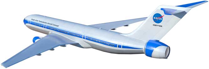
Figure 1 The STARC-ABL aircraft configuration uses a propulsor mounted in the aft of the fuselage that ingests the boundary layer.
2.0 DESIGN OPTIMISATION OF THE AEROPROPULSIVE FUSELAGE
2.1 Aerodynamic model
The aerodynamic analysis consists of solving the RANS equations using ADflow( Reference Lyu, Kenway and Martins 17 ) in a 2D axisymmetric domain. ADflow is a second-order, finite-volume CFD solver that provides adjoint analytic derivatives( Reference Lyu, Kenway, Paige and Martins 18 ). Together with a gradient-based optimisation algorithm, this enables efficient design optimisation with respect to a large number of design variables( Reference Martins and Hwang 19 ). This CFD solver has been extensively validated for transonic flight conditions against wind-tunnel data provided by the 2017 AIAA Drag Prediction Workshop( Reference Coder, Pulliam, Hue, Kenway and Sclafani 20 ), and mesh convergence studies have verified the second-order convergence of the solver for a range of different meshes( Reference Kenway, Secco, Martins, Mishra and Duraisamy 21 ). To simplify the analysis, the STARC-ABL aircraft is separated into fuselage (including the aft propulsor) and lifting surface components. A representative fuselage is sized to be similar to that of a Boeing 737-900 in length and diameter. We consider two fuselage configurations: a BLI configuration and a podded configuration. The podded configuration provides a reference against which we can compare the BLI propulsor performance.
The BLI configuration consists of a single integrated geometry with the propulsor attached to the aft part of the fuselage. Figure 2 shows this configuration with labels for the four boundary conditions: viscous walls (S 1,S 2), outflow face (S 3), and inflow face (S 4). The surfaces S 3 and S 4 represent the interface between the propulsion and aerodynamic models, and appropriate boundary conditions must be applied on these surfaces. The outflow boundary condition on S 3 is a prescribed uniform static pressure. This assumption is consistent with boundary-layer theory, which assumes a constant static pressure at the surface. The total pressure variation caused by the boundary layer and the associated velocity variation is thus carried out of the flow domain as a non-uniform flow at S 3. The inflow boundary condition on S 4 is defined by a prescribed uniform p t and T t, which ultimately is defined by the propulsion model, so while the outflow condition allows for flow non-uniformity, the inflow condition does not. This means that the model assumes that the flow exiting the fan is well mixed. The mesh for this axisymmetric analysis has 170,000 cells, and each CFD solution takes approximately 2 min when using a quad-core workstation with 2.8GHz processors.
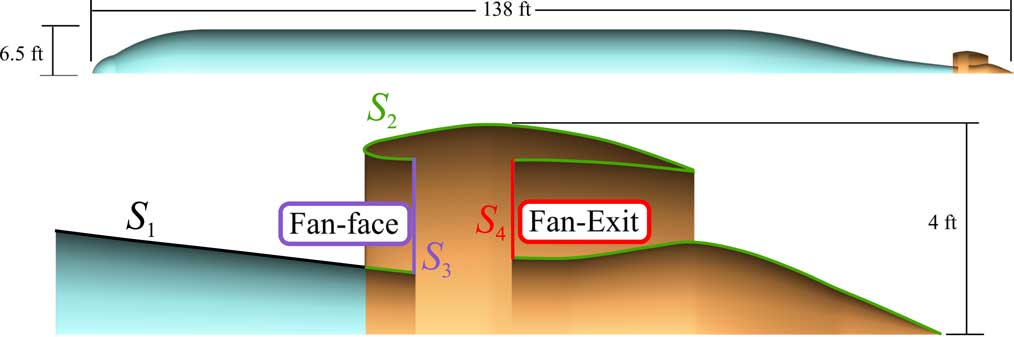
Figure 2 BLI configuration and boundary conditions: viscous walls (S 1,S 2), outflow face (S 3), and inflow face (S 4)
The podded configuration consists of two separate surfaces: one for the fuselage and another for the podded propulsor. Figure 3 shows each of these surfaces. The main body of the fuselage is identical in both configurations. Similarly, the nacelle shape and plug shape are also identical for the two configurations. The bare propulsor model performance predictions are used to estimate the under-wing propulsor performance as well.

Figure 3 The podded configuration serves as a reference and models fuselage (top) and propulsor (bottom) separately.
For both configurations, the geometry is parameterised via free-form deformation (FFD) to modify the surface mesh( Reference Kenway, Kennedy and Martins 22 ). The surface changes are propagated to the volume grid using an inverse distance weighted method of mesh deformation( Reference Luke, Collins and Blades 23 ). The majority of the fuselage shape remains fixed, but the shape of the aft taper section and of the nacelle and plug are allowed to vary. The FFD boxes and associated control points are shown in Fig. 4 for the BLI configuration. The podded configuration uses the same FFD on the propulsor section (shown in orange) but keeps the clean fuselage unchanged.

Figure 4 The shape of the BLI configuration is enveloped in FFD boxes (black lines) and parameterised using FFD control points.
One of the major challenges when modelling BLI propulsion systems is establishing a consistent scheme for bookkeeping all of the forces on the combined aeropropulsive system when some of the forces are computed by the aerodynamic analysis and other forces are computed by the propulsion analysis. We avoid this problem by computing all the forces within only the aerodynamic analysis using the following equation:
 $$C_{{F_{x} }} {\equals}{2 \over {{\rm \rho }_{\infty} V_{\infty}^{2} A_{{{\rm ref}}} }}\left( \matrix{\it \int\int_{S_{1} } \left( {p{\mib{\hat{n}}} {\plus}{\mib{f}} _{{{\rm visc}}} } \right) \cdot {\mib{\hat{x}}} {d}S{\plus}\int \int_{S_{2} } \left( {p{\mib{\hat{n}}} {\plus}{\mib{f}} _{{{\rm visc}}} } \right) \cdot {\mib{\hat{x}}} {\rm d}S \hfill \cr {\plus}\int \int_{S_{3} } \left( {p{\mib{\hat{n}}} \cdot {\mib{\hat{x}}} {\plus}{\rm \rho }_{3} u_{3}^{2} } \right){\rm d}S{\plus}\int \int_{S_{4} } \left( {p{\mib{\hat{n}}} \cdot {\mib{\hat{x}}} {\minus}{\rm \rho }_{4} u_{4}^{2} } \right){\it d}S \hfill \cr} \right),$$
which accounts for all of the viscous, pressure, and momentum flux forces on the entire body. Each contribution is colour coded to match the associated boundary condition in Fig. 2. Note that the sign of
 $$C_{{F_{x} }} $$
is significant: a positive value indicates a net decelerating force (i.e. drag) on the body, and a negative value indicates a net accelerating force (i.e. thrust). The reference values used for Equation (2) are given in Table 1.
$$C_{{F_{x} }} $$
is significant: a positive value indicates a net decelerating force (i.e. drag) on the body, and a negative value indicates a net accelerating force (i.e. thrust). The reference values used for Equation (2) are given in Table 1.
Table 1 Reference values used in the force non-dimensionalisation
2.2 Propulsion model
The propulsion analysis is performed using a 1D thermodynamic model implemented in pyCycle( Reference Gray, Chin, Hearn, Hendricks, Lavelle and Martins 24 , Reference Hearn, Hendricks, Chin, Gray and Moore 25 ), a modular thermodynamic cycle modelling tool built in OpenMDAO( Reference Gray, Hearn, Moore, Hwang, Martins and Ning 15 ). This tool provides a flexible cycle modelling capability similar to the industry standard NPSS( Reference Jones 26 ) tool; however, unlike NPSS, pyCycle provides analytic derivatives, which were necessary for the gradient-based optimisations that we perform in this work.
The propulsor fan is modelled with three separate parts, as shown in the XDSM diagram(
Reference Lambe and Martins
27
) (Fig. 5). The flow-start computes the enthalpy (h) and entropy (s) given mass flow rate (
 $$\dot{m}$$
), mass-averaged total temperature (
$$\dot{m}$$
), mass-averaged total temperature (
 $$T_{{\rm t}}^{{{\rm FF}}} $$
), and mass-averaged total pressure (
$$T_{{\rm t}}^{{{\rm FF}}} $$
), and mass-averaged total pressure (
 $$p_{{\rm t}}^{{{\rm FF}}} $$
) from the fan face (S
3 in Fig. 2). The fan pressure ratio (FPR) is also given as an input and will be one of the design variables in the optimisation. The model outputs fan exit total temperature (
$$p_{{\rm t}}^{{{\rm FF}}} $$
) from the fan face (S
3 in Fig. 2). The fan pressure ratio (FPR) is also given as an input and will be one of the design variables in the optimisation. The model outputs fan exit total temperature (
 $$T_{{\rm t}}^{{{\rm FE}}} $$
), total pressure (
$$T_{{\rm t}}^{{{\rm FE}}} $$
), total pressure (
 $$p_{{\rm t}}^{{{\rm FF}}} $$
), and the required shaft power to handle the given mass flow rate. The fan efficiency is computed using a linear correlation with FPR
$$p_{{\rm t}}^{{{\rm FF}}} $$
), and the required shaft power to handle the given mass flow rate. The fan efficiency is computed using a linear correlation with FPR
 $${\rm \eta }_{{\rm a}} {\equals}1.066 {\minus} 0.0866 \cdot {\rm FPR},$$
where the constants were chosen to yield a 96.2% efficiency for FPR=1.2 and 95% efficiency for FPR=1.4. This linear fit for fan adiabatic efficiency is derived from data published in two studies on next-generation subsonic transport aircraft for the NASA Advanced Air Transport Technologies Project( Reference Greitzer, Bonnefoy, la Rosa Blanco, Dorbian, Drela, Hall, Hansman, Hileman, Liebeck, Lovegren, Mody, Pertuze, Sato, Spakovszky, Tan, Hollman, Duda, Fitzgerald, Houghton, Kerrebrock, Kiwada, Kordonowy, Parrish, Tylko, Wen and Lord 28 , Reference Bradley and Droney 29 ). Equation (3) captures the change in fan performance as the design FPR changes, but it does not account for the impact of inlet distortion caused by the BLI. The 2D aerodynamic analysis used here does not accurately capture inlet distortion, so the impact of distortion is not modelled in this work. Ongoing work with 3D aerodynamic models will account for this impact( Reference Gray, Kenway and Martins 30 ).
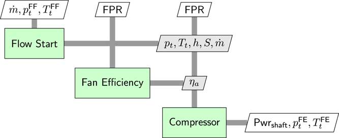
Figure 5 The propulsor fan model consists of three sub-models. It computes the shaft power and fan exit conditions given the FPR, mass flow, and fan face conditions.
2.3 Optimisation problem
To capture the aeropropulsive interactions, we build a fully coupled model of the fuselage and BLI propulsor by combining the aerodynamic and propulsion models in the OpenMDAO framework. OpenMDAO was selected for several reasons. As mentioned above, the pyCycle tool itself is built in OpenMDAO, which makes the framework the natural choice for the larger multidisciplinary integration. In addition, OpenMDAO supports an MPI-based, distributed memory data storage that is necessary to efficiently integrate the ADflow aerodynamics analysis. Lastly, both ADflow and pyCycle provide analytic derivatives, and OpenMDAO is able to automatically compute the multidisciplinary adjoint derivatives for the coupled model, which saves development time for our application. The availability of adjoint analytic derivatives enables us to use efficient gradient-based optimisation to handle the high-dimensional design space of the combined aeropropulsive design problem. In this work, we use a sequential quadratic programming (SQP) optimiser implemented in the SNOPT( Reference Gill, Murray and Saunders 31 ) package, which is integrated into the OpenMDAO framework via the pyOptSparse Python wrapper( Reference Perez, Jansen and Martins 32 ).
The aeropropulsive coupling is implemented using an individual design feasible (IDF) optimisation architecture(
Reference Martins and Lambe
33
), which uses constraints imposed on the final solution to enforce multidisciplinary compatibility. There are four IDF constraints represented by
 $${\scr R}\left( {{\rm Pwr}} \right)$$
and
$${\scr R}\left( {{\rm Pwr}} \right)$$
and
 $${\scr R}\left( {{\rm B}{\rm .C}{\rm .}} \right)$$
in Fig. 6 that force the target values − any value with the ()* superscript − to match the values computed using the actual models. We use the same optimisation problem formulation for both the BLI and the podded configurations. The grids for the aerodynamic analysis are different between the two configurations, as shown in Fig. 2 (BLI configuration) and Fig. 3 (podded configuration).
$${\scr R}\left( {{\rm B}{\rm .C}{\rm .}} \right)$$
in Fig. 6 that force the target values − any value with the ()* superscript − to match the values computed using the actual models. We use the same optimisation problem formulation for both the BLI and the podded configurations. The grids for the aerodynamic analysis are different between the two configurations, as shown in Fig. 2 (BLI configuration) and Fig. 3 (podded configuration).
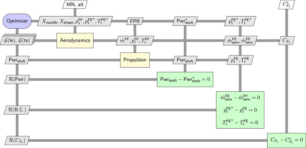
Figure 6 XDSM diagram of the full optimisation problem formulation, including the compatibility constraints that enforce the aeropropulsive coupling.
The goal of the optimisation is to minimise Pwrshaft with respect to FPR, static pressure at the fan face
 $$\left( {p_{s}^{{{\rm FF}}} } \right)$$
, and 311 aerodynamic shape variables (X
nacelle, X
shape), subject to a prescribed net force
$$\left( {p_{s}^{{{\rm FF}}} } \right)$$
, and 311 aerodynamic shape variables (X
nacelle, X
shape), subject to a prescribed net force
 $$\left( {C_{{F_{x} }}^{{\asterisk}} } \right)$$
on the fuselage. The FPR is allowed to vary from 1.2 to 1.5. These bounds are applied to keep the fan designs within a reasonable range. The shape variables have no upper bound but are given lower bounds based on the limits of the mesh deformation algorithm. Specifically, the lower limits prevent the nozzle plug from being forced to shrink below a minimum radius.
$$\left( {C_{{F_{x} }}^{{\asterisk}} } \right)$$
on the fuselage. The FPR is allowed to vary from 1.2 to 1.5. These bounds are applied to keep the fan designs within a reasonable range. The shape variables have no upper bound but are given lower bounds based on the limits of the mesh deformation algorithm. Specifically, the lower limits prevent the nozzle plug from being forced to shrink below a minimum radius.
The optimisation problem formulation is detailed in Table 2. In addition to the design variables mentioned above, there are three additional design variables listed in Table 2: Pwrshaft,
 $$p_{{\rm t}}^{{{\rm FE{\asterisk}}}} $$
, and
$$p_{{\rm t}}^{{{\rm FE{\asterisk}}}} $$
, and
 $$T_{{\rm t}}^{{{\rm FE{\asterisk}}}} $$
); however, these are not true design degrees of freedom because they are used by the optimiser to satisfy the IDF constraints. Two sets of geometric constraints (
$$T_{{\rm t}}^{{{\rm FE{\asterisk}}}} $$
); however, these are not true design degrees of freedom because they are used by the optimiser to satisfy the IDF constraints. Two sets of geometric constraints (
 $${\cal G}_{{{\rm LE}}} $$
and
$${\cal G}_{{{\rm LE}}} $$
and
 $${\cal G}_{{{\rm TE}}} $$
) are imposed on the leading and the trailing edge of the propulsor nacelle profile to ensure that the optimiser does not make them unrealistically thin.
$${\cal G}_{{{\rm TE}}} $$
) are imposed on the leading and the trailing edge of the propulsor nacelle profile to ensure that the optimiser does not make them unrealistically thin.
Table 2 Optimisation problem for the fuselage aeropropulsive design

In Fig. 6, the
 $$C_{{F_{x} }} $$
constraint appears similar to the four IDF constraints, except that the target value (
$$C_{{F_{x} }} $$
constraint appears similar to the four IDF constraints, except that the target value (
 $$C_{{F_{x} }}^{{\asterisk}} $$
) is given as a parameter external to the optimisation. This constraint is not needed for multidisciplinary compatibility, but instead, it is used to ensure a well-posed optimisation problem. This constraint is needed because we do not know a priori what the relative size of the BLI and under-wing propulsors should be. Depending on what the optimal sizing turns out to be, the net force on the fuselage could range from a net drag to a net thrust. Because we do not know the thrust split, a constraint on net force is required in order to ensure a unique solution to the design optimisation problem.
$$C_{{F_{x} }}^{{\asterisk}} $$
) is given as a parameter external to the optimisation. This constraint is not needed for multidisciplinary compatibility, but instead, it is used to ensure a well-posed optimisation problem. This constraint is needed because we do not know a priori what the relative size of the BLI and under-wing propulsors should be. Depending on what the optimal sizing turns out to be, the net force on the fuselage could range from a net drag to a net thrust. Because we do not know the thrust split, a constraint on net force is required in order to ensure a unique solution to the design optimisation problem.
In the first phase of this work, we perform a sweep of optimisations for a range of
 $$C_{{F_{x} }}^{{\asterisk}} $$
values. In the second phase, using the data from these optimisations, we find the most efficient size for the BLI propulsor.
$$C_{{F_{x} }}^{{\asterisk}} $$
values. In the second phase, using the data from these optimisations, we find the most efficient size for the BLI propulsor.
2.4 Aeropropulsive optimisation results
Two sets of 13 optimisations are performed for different net thrust constraint values, ranging from
 $$C_{{F_{x} }}^{{\asterisk}} {\equals}0.0025$$
to
$$C_{{F_{x} }}^{{\asterisk}} {\equals}0.0025$$
to
 $$C_{{F_{x} }}^{{\asterisk}} {\equals}{\minus}0.156$$
, corresponding to 3,000N net drag and 17,000N net thrust, respectively. One set of optimisations is run on the BLI configuration, and a second set is run on the podded configuration to serve as a reference. All of the optimised configurations had an FPR of 1.2, which was the lower bound for that design variable. The PSC, defined in Equation (1), is computed for each net thrust coefficient value by using the shaft power for the optimised podded configuration as the reference (
$$C_{{F_{x} }}^{{\asterisk}} {\equals}{\minus}0.156$$
, corresponding to 3,000N net drag and 17,000N net thrust, respectively. One set of optimisations is run on the BLI configuration, and a second set is run on the podded configuration to serve as a reference. All of the optimised configurations had an FPR of 1.2, which was the lower bound for that design variable. The PSC, defined in Equation (1), is computed for each net thrust coefficient value by using the shaft power for the optimised podded configuration as the reference (
 $${\rm Pwr}_{{{\rm shaft}}}^{'} $$
). Figure 7 shows that the PSC takes a maximum value of 0.202 for
$${\rm Pwr}_{{{\rm shaft}}}^{'} $$
). Figure 7 shows that the PSC takes a maximum value of 0.202 for
 $$C_{{F_{x} }} {\equals}0.0025$$
and that the PSC decreases smoothly to 0.093 for
$$C_{{F_{x} }} {\equals}0.0025$$
and that the PSC decreases smoothly to 0.093 for
 $$C_{{F_{x} }} {\equals}{\minus}0.156$$
. At
$$C_{{F_{x} }} {\equals}{\minus}0.156$$
. At
 $$C_{{F_{x} }} {\equals}0.0025$$
, there is a slight net decelerating force on the fuselage, which corresponds to a small BLI propulsor. Conversely,
$$C_{{F_{x} }} {\equals}0.0025$$
, there is a slight net decelerating force on the fuselage, which corresponds to a small BLI propulsor. Conversely,
 $$C_{{F_{x} }} {\equals}{\minus}0.156$$
yields a net accelerating force on the fuselage, which corresponds to a larger BLI propulsor. Note that the results in Fig. 7 are computed only on the fuselage and BLI propulsor. In the next section, we extend this problem to estimate the sizing for the whole propulsion system, including the under-wing propulsors.
$$C_{{F_{x} }} {\equals}{\minus}0.156$$
yields a net accelerating force on the fuselage, which corresponds to a larger BLI propulsor. Note that the results in Fig. 7 are computed only on the fuselage and BLI propulsor. In the next section, we extend this problem to estimate the sizing for the whole propulsion system, including the under-wing propulsors.
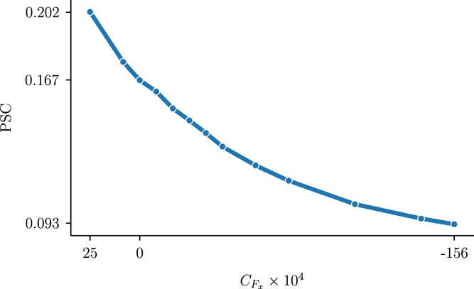
Figure 7 Power saving coefficient vs
 $$C_{{F_{x} }} $$
shows that smaller BLI propulsors (small positive
$$C_{{F_{x} }} $$
shows that smaller BLI propulsors (small positive
 $$C_{{F_{x} }} $$
) offer greater power savings than larger ones.
$$C_{{F_{x} }} $$
) offer greater power savings than larger ones.
3.0 BLI PROPULSOR SIZING ANALYSIS
3.1 Podded propulsor performance
Although traditional thrust and drag accounting is not valid for the BLI configuration, the podded configuration can still be examined using a force-based metric because in that case, the propulsor and fuselage are two separate items; thus, the propulsor thrust (
 $$C_{{F_{{{\rm pod}}} }} $$
) is a well-defined quantity, computed using Equation (2) applied to the podded propulsor surfaces (the orange surfaces in Fig. 3). Figure 8 plots the data for each of the optimised podded propulsors normalised by counts of net force on the propulsor. Given that FPR=1.2 for all of the optimised configurations, from a pure thermodynamic cycle analysis perspective, one would expect a flat line in Fig. 8; however, since the thrust data computed here includes the nacelle drag it represents installed thrust and some dependence on nacelle diameter is expected.
$$C_{{F_{{{\rm pod}}} }} $$
) is a well-defined quantity, computed using Equation (2) applied to the podded propulsor surfaces (the orange surfaces in Fig. 3). Figure 8 plots the data for each of the optimised podded propulsors normalised by counts of net force on the propulsor. Given that FPR=1.2 for all of the optimised configurations, from a pure thermodynamic cycle analysis perspective, one would expect a flat line in Fig. 8; however, since the thrust data computed here includes the nacelle drag it represents installed thrust and some dependence on nacelle diameter is expected.
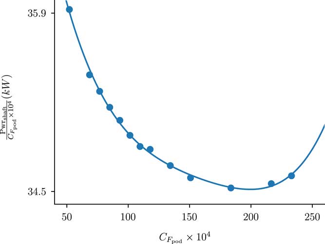
Figure 8
 $${\rm Pwr}_{{{\rm shaft}}} \,/\,C_{{F_{{{\rm pod}}} }} $$
data (circles) and fourth-order polynomial fit (solid line) for the podded propulsor.
$${\rm Pwr}_{{{\rm shaft}}} \,/\,C_{{F_{{{\rm pod}}} }} $$
data (circles) and fourth-order polynomial fit (solid line) for the podded propulsor.
The solid line in Fig. 8 is a fourth-order polynomial fit of the data, given by
 $${{\rm Pwr_{{{\rm shaft}}} } \over {C_{{F_{{{\rm pod}}} }} {\times}10^{4} }}{\equals}38.89{\minus}0.00867x{\plus}7.474{\times}10^{{{\minus}4}} x^{2} {\minus}3.013{\times}10^{{{\minus}6}} x^{3} {\plus}4.729{\times}10^{{{\minus}9}} x^{4} .$$
This equation can be used to predict the required shaft power. For any podded engine thrust value, we should stay within the bounds of the fitted data to avoid extrapolation issues. One caveat with this equation is that it was fit based on results from a single under-wing propulsor, so when applying it to compute power requirements for the whole aircraft, it is important to consider that there are two engines and hence each one only produces half the thrust and hence half the force coefficient.
3.2 Propulsion system sizing method
Equation (2) computes only the force coefficient on the fuselage component of the aircraft. To size the propulsion system, we must consider additional drag contributions from the lifting surfaces−wings, vertical tail, and horizontal tail. This lifting surface drag is computed using the empirical drag methods in the FLOPS tool( Reference McCullers 34 ), using appropriate inputs for the STARC-ABL configuration. In this case, FLOPS predicts a lifting surface drag of 216 counts (C D =0.0216).
At a steady cruise condition, the aircraft should remain at a constant speed, meaning that the net force is zero. With the assumed C
D
and any prescribed value of
 $$C_{{F_{x} }} $$
, we can compute the required additional force coefficient from the under-wing propulsors that satisfy this zero-net-force constraint as follows:
$$C_{{F_{x} }} $$
, we can compute the required additional force coefficient from the under-wing propulsors that satisfy this zero-net-force constraint as follows:
 $$C_{{F_{{{\rm pod}}} }} {\equals}{\minus}(C_{D} {\plus}C_{{F_{x} }} ),$$
where, as previously mentioned, the sign of the force coefficients is significant: positive values result in deceleration and negative impart acceleration.
By combining Equations (4) and (5), we compute the required shaft power from the under-wing propulsors. To provide a reference, we use the net drag on the clean fuselage from the podded configuration and assume that 100% of the thrust − and hence all of the required shaft power − is generated by the under-wing engines. For each optimised BLI fuselage design, the
 $$C_{{F_{x} }} $$
is known because it is prescribed as an optimisation constraint; therefore, the required additional shaft power from the under-wing propulsors can be computed using Equation (5) for each BLI configuration. To compute the total required shaft power for the BLI configuration at cruise, we can use the following relationship:
$$C_{{F_{x} }} $$
is known because it is prescribed as an optimisation constraint; therefore, the required additional shaft power from the under-wing propulsors can be computed using Equation (5) for each BLI configuration. To compute the total required shaft power for the BLI configuration at cruise, we can use the following relationship:
 $${\rm Pwr}_{{{\rm tot}}} {\equals}{{{\rm Pwr}_{{{\rm BLI}}} } \over {{\rm \eta }_{{{\rm trans}}} }}{\plus}{\rm Pwr}_{{{\rm pod}}} ,$$
where we take into account the combined transmission efficiency, ηtrans. This is the efficiency of the system that generates the power from the under-wing engines and transmits it to the aft fuselage to power the electric drive motor. Three values for ηtrans are considered: 0.9, 0.95, and 0.98. An ηtrans of 0.9 represents the expected transmission efficiency for a traditional AC/DC power system(
Reference Welstead and Felder
11
). The values for ηtrans of 0.95 and 0.98 are assumed for future performance of systems based on the use of superconducting motors, generators, and power lines. The percentage reduction in power consumption at cruise for a fuselage with a particular
 $$C_{{F_{x} }} $$
and assumed ηtrans can then be computed by taking the ratio of the power required for the BLI configuration to the reference power required for the configuration without BLI (the podded configuration).
$$C_{{F_{x} }} $$
and assumed ηtrans can then be computed by taking the ratio of the power required for the BLI configuration to the reference power required for the configuration without BLI (the podded configuration).
3.3 Propulsion sizing results
Figure 9 shows the combined results from the analysis described by Equations (4), (5), and (6) plotted versus the power split between the aft BLI propulsor and the under-wing propulsors. The results show that the optimal propulsor sizing depends strongly on the assumed value for ηtrans. Assuming current power transmission technology levels (i.e. ηtrans=0.9), BLI yields a 1% reduction in net shaft power required at cruise, and the aft propulsor uses 15.3% of the total power. This small improvement in overall performance is significantly lower than the 9–20% improvement in the standalone BLI propulsor as seen in Fig. 7. This makes it clear that ηtrans is having a massive effect on overall system performance. Losing 10% of the power by converting mechanical energy to electrical and back to mechanical is driving the overall system to a very small BLI propulsor, which is limiting the overall effect on overall fuel burn.
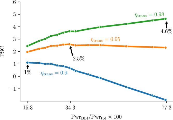
Figure 9 Overall aircraft PSC at cruise vs the fraction of shaft power used for BLI at different assumed values of transmission efficiency, ηtrans.
As ηtrans improves, the overall results improve as well. For ηtrans=0.95, PSC values of 2–2.5% are achieved across the whole range of power splits. These results are notable for the large flat plateau to the right of the optimum power split of 34.3%, which implies that there is a large amount of design freedom in terms of aft propulsor sizing. In the best case scenario, ηtrans=0.98, the best PSC occurs at the largest power split analysed. At very high ηtrans, this result is expected because the best performance would come from making as much thrust from the BLI propulsor as possible.
We must emphasise that this sizing analysis is done from a purely thermodynamic perspective. The optimum power split between the BLI and under-wing propulsors is estimated considering only the aeropropulsive effects and the overall power usage of the system. Furthermore, only a single cruise condition is examined. A complete aircraft design process would need to consider other factors, including the overall mass of the turboelectric propulsion system with respect to BLI propulsor size, multiple flight conditions, thermal performance for the power transmission system, tail rotation angle at takeoff, and centre of gravity movement. Additionally, the axisymmetric analysis done here does not account for the impact of the wing and tail on the inflow conditions of the BLI propulsor. Despite missing these elements in the analysis, these results do provide a conclusive picture of how the propulsion system performance is affected by the inclusion of a BLI propulsor, and how the optimum sizing of that propulsion system varies with changes in electric power transmission efficiency.
3.4 Qualitative analysis of the optimised configurations
Figure 10 compares the optimal power split designs for ηtrans=(0.9, 0.95, 0.98). The most notable change between the three designs is the size of the aft propulsor, which grows significantly as the assumed transmission efficiency improves. The outermost streamline of the flow entering the propulsor is shown as a black line on each design. For ηtrans=0.98, the propulsor is very large and is clearly ingesting non-boundary-layer flow. Closer examination of the nacelle and nozzle plug shapes between the three cases shows significant differences in shape between each case. The nozzle plug shows the greatest variation in shape, with a nearly flat profile for the smallest propulsor and the development of the ramp shape to create a stronger nozzle throat as the propulsor grows. The nacelle also changes shape, though more subtly. As the nacelle moves up into the faster moving flow, it takes on a slightly larger tilt to better align with the local flow and becomes slightly thicker. These shape variations highlight the importance of using an optimisation-based design approach for this coupled problem. The aerodynamic analysis is sensitive to these small changes in the shape, and hence the overall trends that are reported are sensitive to them as well, and an optimiser is required to make sure each design considered in the parametric sweep is performing as well as it can.
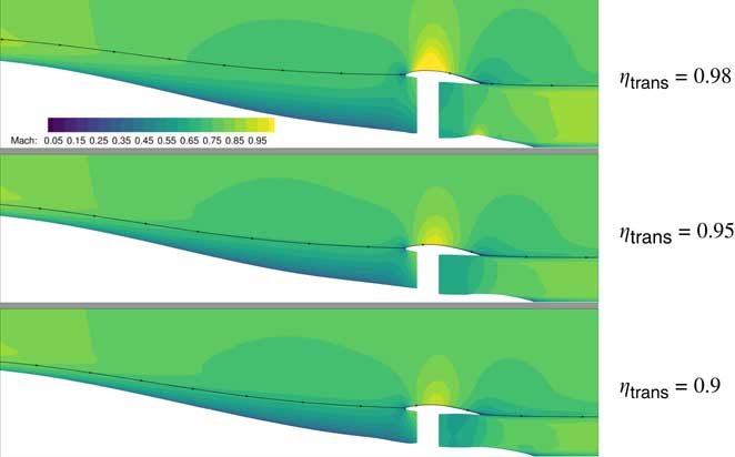
Figure 10 Best-performing designs for three assumed values of ηtrans. Increased transmission efficiency drives the design to larger BLI propulsors relative to the under-wing engines.
The variation in the Mach contours between each design in Fig. 10 is worth discussing. There are two places where these variations are most significant and obvious. The flow over the top of the nacelle changes dramatically as the propulsor grows larger. For ηtrans=0.9, the nacelle is effectively in the shadow of the fuselage and the nacelle wall sees very low-speed flow. As the nacelle grows bigger, the flow becomes faster, and the high-speed region over the top of it grows larger. This variation in flow results in a variation in the amount of viscous drag on the nacelle for the BLI case that is greater than was observed for the podded configuration in clean flow.
The second flow feature that displays variation with changing propulsor is the boundary-layer profile near the inlet of the propulsor. We examined the variation in the flow over the aft fuselage due to the presence of the propulsor in greater detail in prior work(
Reference Gray, Mader, Kenway and Martins
14
); however, that work performed only aeropropulsive analysis for a fixed nacelle shape. Those results indicated that although the flow field was changed with a variation in the inlet height, the trends were sensitive to
 $$p_{{\rm s}}^{{{\rm FF}}} $$
, which we acknowledged could change in a final optimised result if nacelle shape was allowed to change. Figure 11 examines the boundary-layer profiles − defined using the total pressure ratio with freestream − half a meter ahead of the inlet lip for the best design found for each assumed value of ηtrans. Total pressure ratio is used to define the boundary layer, rather than the more traditional velocity metric, because the flow around the tailcone is undergoing inviscid diffusion, which makes a comparison with the freestream velocity inaccurate. The edge of the boundary layer is denoted by the vertical red dashed line at p
t/p
t∞=0.99. In Fig. 11, the largest propulsor design (corresponding to ηtrans=0.98) shows a pronounced difference in boundary-layer profile compared to the two smaller designs. The larger propulsor applies a greater backpressure to the flow, which causes the boundary layer to grow thicker. We can also clearly see from the horizontal dashed lines that denote the inlet height for each design that the largest propulsor ingests a significant amount of flow from outside the boundary layer. The two smaller propulsors, however, ingest only boundary-layer flow. Although the profiles for the two smaller propulsors look very similar, there is a small difference very close to the fuselage where variations in the surface pressure distribution become apparent. Overall, these results show less variation in the boundary-layer profile than prior work, but it is clear that the aeropropulsive coupling still has an impact on the boundary layer near the propulsor.
$$p_{{\rm s}}^{{{\rm FF}}} $$
, which we acknowledged could change in a final optimised result if nacelle shape was allowed to change. Figure 11 examines the boundary-layer profiles − defined using the total pressure ratio with freestream − half a meter ahead of the inlet lip for the best design found for each assumed value of ηtrans. Total pressure ratio is used to define the boundary layer, rather than the more traditional velocity metric, because the flow around the tailcone is undergoing inviscid diffusion, which makes a comparison with the freestream velocity inaccurate. The edge of the boundary layer is denoted by the vertical red dashed line at p
t/p
t∞=0.99. In Fig. 11, the largest propulsor design (corresponding to ηtrans=0.98) shows a pronounced difference in boundary-layer profile compared to the two smaller designs. The larger propulsor applies a greater backpressure to the flow, which causes the boundary layer to grow thicker. We can also clearly see from the horizontal dashed lines that denote the inlet height for each design that the largest propulsor ingests a significant amount of flow from outside the boundary layer. The two smaller propulsors, however, ingest only boundary-layer flow. Although the profiles for the two smaller propulsors look very similar, there is a small difference very close to the fuselage where variations in the surface pressure distribution become apparent. Overall, these results show less variation in the boundary-layer profile than prior work, but it is clear that the aeropropulsive coupling still has an impact on the boundary layer near the propulsor.
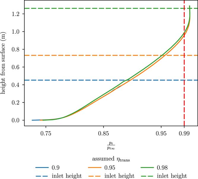
Figure 11 Boundary-layer profiles (measured via p t/p t∞) for the best designs found for each assumed value of ηtrans. The horizontal dashed lines indicate the height of the inlet lip for each design.
4.0 CONCLUSIONS
A series of design optimisations of a simplified version of NASA’s STARC-ABL aircraft configuration were performed using a fully coupled aeropropulsive model. The goal of the STARC-ABL configuration is to utilise an aft-mounted, electrically driven BLI propulsor to achieve a significant reduction in mission fuel burn. The aircraft configuration was simplified by representing the fuselage and aft-mounted propulsor as an axisymmetric body. The aerodynamic model of the fuselage and propulsor combination was based on a RANS CFD model, and this was coupled with a 1D thermodynamic model of the propulsor fan via outflow and inflow boundary conditions that modelled the fan face and the fan exit, respectively. The coupling was formulated using an IDF formulation so that it was enforced as part of the optimisation. The entire model was constructed and optimised using gradient-based optimisation with analytic derivatives in the OpenMDAO framework. The shaft power was minimised, with respect to both aerodynamic shape variables and propulsion design variables while enforcing a prescribed constraint on the net force of the fuselage and propulsor combination. A series of optimisations was performed with different values for the net force constraint for both a BLI and a reference podded configuration for the aft-mounted propulsor.
The performance of the BLI propulsor was measured by comparing the required power of the optimised BLI configuration to that of the optimised podded configuration for the same net force on the overall body (i.e. computing the PSC). This comparison showed that smaller propulsors achieved the best PSC. For small values of net drag on the fuselage, the BLI configuration had a PSC of 0.202. A PSC value of 0.202, or a 20.2% reduction in required shaft power, seemingly represents a significant potential saving; however, this point also corresponds to the smallest BLI propulsor design. The BLI propulsors were found to get progressively less efficient as they grew in size, reaching a minimum power savings coefficient of 0.093 for the largest propulsor.
The variation in PSC as a function of propulsor sizing is significant because it means that the designs with the highest PSC values do not necessarily translate to the best overall design of the propulsion system. This is due to the fact that the STARC-ABL only gets part of its thrust from the aft-mounted BLI propulsor. Despite being significantly more efficient, the smaller BLI propulsors produce a smaller portion of the overall thrust, and hence can only reduce the energy usage of the whole propulsion system by a small amount. In order to identify the best overall design for the whole propulsion system, we performed a propulsion sizing analysis by examining the combined power requirements of both the BLI propulsor, accounting for the effect of power transmission efficiency, and under-wing engines to provide a metric of overall efficiency. The sizing analysis indicated that assuming current electrical power transmission technology, 1% power savings is achieved when 15.3% of the aircraft power is transmitted to the aft propulsor. Using a moderately advanced power transmission system with an efficiency of 95%, the optimum PSC reaches 2.5%. For an extremely high power transmission efficiency of 98%, the best performance is achieved by making as much thrust as possible from the BLI propulsor.
The aeropropulsive analysis and design performed for this work demonstrates the importance of using fully coupled models to predict the performance of physically coupled systems. The standalone BLI propulsor analysis shows a large potential efficiency gain from this aeropropulsive concept. The challenge is to integrate BLI technology into an aircraft configuration to make the most of it. Analysis of the full propulsion system for the STARC-ABL configuration shows that propulsion–airframe integration will have a large impact on the overall performance. There are two key coupling effects that each affect how the full propulsion system performs. First, the aeropropulsive effects on the BLI propulsor are shown to vary in strength as a function of propulsor sizing which, contributes to a non-linear variation in BLI benefit. Second, the impact of electrical power transmission efficiency is shown to have a first-order effect on the relative sizing of the under-wing vs BLI propulsors. Although they can be described separately, in reality, these two coupling effects cannot be considered in isolation from each other in the context of aeropropulsive design. As one varies the power transmission efficiency, the propulsion system must be redesigned to maximise benefits and the relative sizing of the under-wing and BLI propulsors can vary significantly.
Acknowledgements
We would like to thank NASA Aeronautics Research Mission Directorate Advanced Air Transport Technologies (AATT) and Transformation Tools and Technologies (TTT) projects for funding this research. We would like to acknowledge the valuable discussions with James Felder and Jason Welstead regarding important details of the STARC-ABL configuration. We would also like to thank Charles Mader, Gaetan Kenway, and John Hwang for providing technical advice through many insightful conversations regarding the aeropropulsive coupling and integration of ADflow into OpenMDAO. Lastly, we would like to acknowledge Bret Naylor, Ken Moore, and Herb Schilling, who developed many of the features in the OpenMDAO framework that were necessary to perform this study.


