3. Results

Our investigation was based on numerical integration of (2.3) in a domain $(x, y) \in [0, 2 {\rm \pi}]^{2}, z \in [-{\rm \pi} , 0]$ with periodic boundary conditions in the $x$ and $y$ directions and with rigid lids on the top and bottom, i.e. velocity boundary conditions on top ($z=0$) and bottom ($z=-{\rm \pi}$) were free slip for $\boldsymbol {v}$ and impenetrability for $w$. The simulations were performed using a dealiased pseudospectral code with $384^{3}$ grid points. We used $\alpha =20$ and $Ro=0.1$ for the numerical experiments reported below, although we found that the qualitative phenomenology and energy transfer directions were similar in neighbouring regimes. Hyperdissipation terms of the form $\nu {\rm \Delta} _{3D}^{8} \boldsymbol {v}$, $\nu {\rm \Delta} _{3D}^{8} w$ and $\nu {\rm \Delta} _{3D}^{8} b$, where ${\rm \Delta} _{3D}= \partial ^{2}/\partial x^{2} + \partial ^{2}/\partial y^{2} + \partial ^{2}/\partial z^{2}$, were added to the right-hand sides of (2.3a), (2.3b) and (2.3c) to dissipate energy reaching grid scale and to increase the range of inviscid scales we resolve. Based on multiple iterative simulations, we set hyperviscosity values ranging from $\nu = 10^{-29}$ to $\nu = 10^{-31}$ for different parameter regimes.

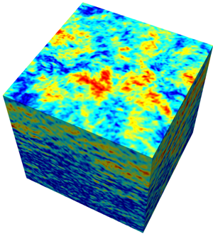
Prior to our wave-balance interaction experiments, we first simulated (2.3) with purely balanced initial conditions for long enough so as to get a matured turbulent geostrophic flow field. Specifically, we simulated (2.3) initializing only the geostrophic balanced field at low wavenumbers, $k \leq 6$, with random numbers assigned to each wavenumber. An example final state of such a balance-only initialized simulation with ${{{{E}}_{{G}}}}(t=0) = 1$ is shown in figure 1$(a)$. Observe the presence of large domain scale vortices. Figure 1$(b)$ shows the time evolution of balanced energy for this particular simulation. Overall we find that in this experiment, that lasted several thousand eddy turn over time scales, less than $1\,\%$ of the balanced energy was dissipated by final time. Figures 1$(c)$ and 1$(d)$ show the horizontal and vertical energy spectra of balanced flows and wave fields at the final time. Although the initial condition was purely in geostrophic balance, weak waves are generated as the flow evolves. Nevertheless, these weak waves and other ageostrophic contributions remain insignificant, as seen in the energy spectra in figures 1$(c)$ and 1$(d)$ showing wave energy spectrum being several orders of magnitude below balanced flow's spectrum.

Figure 1. Panel $(a)$ shows geostrophic vorticity ${{{\zeta }}_{{G}}}$ at $t=4000$. The top surface in the figure is the horizontal plane $z=-h$, where $h={\rm \pi} /100$. Panel $(b)$ shows the time series of the fractional change in balanced energy, $({{{{E}}_{{G}}}}(t) - E(0))/{{{{E}}_{{G}}}}(0)$. Panel $(c)$ shows the horizontal energy spectra $\hat {E}( k_h)$ of the wave and balanced flow on the horizontal plane $z=-h$ at $t=4000$. Finally, panel $(d)$ shows the vertical energy spectrum of the horizontally averaged energy $\hat {E}( k_z)$ associated with the wave and balanced flow at $t=4000$. The spectral slopes shown above were calculated based on a best fit in the range $k=10\text{--}50$.

We used simulations such as those described above to get matured turbulent geostrophic flow fields with energy values of our choice. On top of this balanced flow we added NIWs with specific energy levels. We initialized NIWs by setting ${{{u}}_{{W}}} = A(z), \ {{{v}}_{{W}}} = {{{w}}_{{W}}} = {{{b}}_{{W}}}=0$, where $A(z) = c_0 \exp (- z^{2}/2 h^{2})$, $c_0$ being a constant which was chosen such that the wave energy ${E}_{W}$ had a specific initial value for each experiment and $z=-h$ is the location where inertial shear, $\textrm {d} A/\textrm {d} z$, is maximum (for the specific experiments discussed below, we set $h={\rm \pi} /100$). This initial condition, which is homogeneous in horizontal space to mimic large scales of the wave field, will generate inertial oscillations as ${{{u}}_{{W}}} + \textrm {i} {{{v}}_{{W}}} = A(z) \exp (-\textrm {i}t), \ {{{w}}_{{W}}} = {{{b}}_{{W}}}= {{{p}}_{{W}}} = 0$, which is an exact solution of the linear wave equations given in (2.5). Furthermore, this horizontally homogeneous inertial oscillation by itself (i.e. in the absence of a balanced flow) satisfy the full set of nonlinear equations (2.3) exactly. Therefore, horizontally homogeneous pure inertial oscillations will retain their state and remain confined to the upper ocean in the absence of a balanced flow.

We integrated (2.3) with the initial conditions being a combination of NIWs and balanced flow as discussed above and, based on our exploratory simulations, we will present three cases in detail and then briefly discuss the changes in neighbouring regimes at the end of this section. The first regime we will examine corresponds to the case where wave and balanced energies have comparable strengths. We identify this as the comparable wave (CW) regime and initialized the flow with ${E}_{W} = {{{{E}}_{{G}}}} = 1$ so that ${ ( {{{{E}}_{{G}}}}/ {E}_{W} ) }_{t=0}=1$. The second regime we will focus on was initialized with ${E}_{W} = 1$, ${{{{E}}_{{G}}}} = Ro^{2}$ so that ${ ( {{{{E}}_{{G}}}}/ {E}_{W} ) }_{t=0} = Ro^{2}$ and will be identified as the strong wave (SW) regime in this work. Finally, for the purposes of comparison, we examine a regime where the balanced flow was not initialized, i.e. ${E}_{W} = 1$, ${{{{E}}_{{G}}}} = 0$ resulting in ${ ( {{{{E}}_{{G}}}}/ {E}_{W} ) }_{t=0} = 0$ and we identify this as the only wave (OW) regime.

For the three regimes described above, figures 2$(a{,}c{,}e)$ and 2$(b{,}d{,}f)$ show the spatial structure of geostrophic vorticity ${{{\zeta }}_{{G}}}$ and the waves’ speed ${U}_{W} = \sqrt { u_{{W} }^{2} + v_{{W} }^{2}}$, respectively. Figures 2$(a{,}b)$, 2$(c{,}d)$ and 2$(e{,}f)$ correspond to the CW, SW and OW regimes, respectively. In the CW regime we found that the balanced vortices continued to merge and become larger, similar to the phenomenology expected in quasi-geostrophic turbulence. A snapshot of such a state is shown in figure 2$(a)$. Although NIWs are initially homogeneous in the horizontal direction and are confined to the upper ocean, the balanced flow imprints its spatial scales on the wave field. Consequently, the wave field acquires small scales and propagates vertically. Figure 2$(b)$ shows the spatial structure of the wave speed at the same time as figure 2$(a)$. Observe that the wave field consists of small scales and is spread across the whole ocean depth. Therefore, the CW regime is characterized by waves developing small scales and rapidly propagating in the vertical direction.

Figure 2. Physical fields in the three regimes at $t=2000$. Panels $(a{,}b)$, $(c{,}d)$ and $(e{,}f)$ show CW, SW and OW regimes, respectively. Panels $(a),(c)$ and $(e)$ show geostrophic vorticity while $(b)$, (d) and $(\,f)$ show wave speed. In all cases the top surface is the plane $z=-h$.

When contrasted with the CW regime, we find significant differences in the SW regime shown in figures 2(c) and 2(d). At early times we observed that the interaction with waves resulted in breaking up of vortices, generating a wide range of small-scale structures in the balanced flow. Qualitatively similar turbulence phenomenology characterized by waves breaking up vortices was seen in the two-dimensional experiments described in Thomas & Yamada (Reference Thomas and Yamada2019) and Thomas & Arun (Reference Thomas and Arun2020). In our experiments in the SW regime, although waves facilitated the generation of small-scale features in the balanced flow, the small-scale vortices were seen to gradually merge. Such an intermediate state of the balanced flow is shown in figure 2$(c)$. Note the small-scale structures and the vortices showing tendencies to merge. In comparison to the CW regime, the wave field in the SW regime is relatively less modulated by the balanced flow. As seen in figure 2$(d)$ showing the spatial structure of waves, the inhomogeneities in the NIW field is much less in this regime relative to the CW regime, in addition to a weaker vertical propagation of waves.

Finally, figures 2$(e)$ and 2$(f)$ show the OW case. The balanced flow, which was not initialized in this case, remains zero at all times as can be seen in figure 2$(e)$ showing geostrophic vorticity. Additionally, the wave field remains as horizontally homogeneous inertial oscillations with no vertical propagation (figure 2$f$). As pointed out earlier, spatially homogeneous inertial oscillations, in the absence of a geostrophic flow, is an exact solution of the full Boussinesq equations (2.3). We included figures 2$(e)$ and 2$(f)$ above to demonstrate that the numerical integration retains features of exact solutions of the Boussinesq equations (apart from a small amount of wave energy being lost to small-scale viscous dissipation in the OW regime) and to emphasis the stark contrast in wave and balanced fields seen in figures 2$(a)$–2$(\,f)$.

We complement the three-dimensional wave speed plots shown in figures 2$(b)$, 2$(d)$ and 2$(\,f)$ with figure 3$(a)$ that shows the vertical structure of horizontally averaged wave kinetic energy at $t=2000$. Note that the wave field in the OW case retains its initial structure, and remains confined to the upper ocean (as inferred from figure 2$f$), while the SW case shows some vertical propagation leading to a decrease in the magnitude of wave energy in the upper ocean relative to the OW case. On the other hand, the CW case shown in figure 3$(a)$ is seen to have relatively negligible energy in the upper ocean, concomitant with the rapid vertical propagation seen in figure 2$(b)$. A further detail associated with wave energy is given in figure 3$(b)$, which shows the time evolution of wave kinetic energy contained in the horizontally homogeneous mode $k_h = 0$. Recall that the wave field in all regimes were initialized as pure inertial oscillations, with energy only in the $k_h = 0$ mode. Therefore, figure 3$(b)$ shows how the energy in pure inertial oscillations changes with time. Note that the OW case shows only a minor drop in energy, this energy drop being due to viscous dissipation at small vertical scales. The wave field in this case retains its initial features and remains as horizontally homogeneous inertial oscillations. The SW case on the other hand is seen to exhibit much more loss in inertial oscillations energy, primarily due to energy conversion to horizontally inhomogeneous NIWs – a mechanism that is absent in the OW case. On a relative comparison, most efficient conversion of energy from pure inertial oscillation mode $k_h = 0$ to inhomogeneous wave modes $k_h \neq 0$ is seen in figure 3$(b)$ to take place in the CW regime.

Figure 3. Panel $(a)$ shows the vertical structure of horizontally averaged wave kinetic energy in the top one-tenth of the domain at $t=2000$, the same time corresponding to the physical plots of the wave field shown in figure 2$(b{,}d{,}f)$. Panel $(b)$ shows the time evolution of kinetic energy of inertial oscillations, i.e. the horizontally homogeneous Fourier mode, in all three regimes.

Our comparison of the CW and SW regimes with the OW regime above highlights the dominant role the strength of the balanced flow has on NIWs. The OW regime with ${ ( {{{{E}}_{{G}}}}/ {E}_{W} ) }_{t=0} = 0$ is characterized by NIWs retaining their initial features, being confined to the upper ocean and remaining spatially homogeneous. Except for a small amount of viscous dissipation, the wave field in the OW regime remains as pure inertial oscillations. The SW regime with ${ ( {{{{E}}_{{G}}}}/ {E}_{W} ) }_{t=0} = Ro^{2}$ was seen to have waves becoming horizontally inhomogeneous and propagating vertically to a certain extent. Finally, the most extreme effects of balanced flow on waves were seen in the CW regime with ${ ( {{{{E}}_{{G}}}}/ {E}_{W} ) }_{t=0} = 1$, where the wave field acquired smaller horizontal scales and exhibited significant vertical propagation to ocean depths. Since all these regimes were initialized with the same wave energy, their inter-comparison reveals that stronger balanced flow leads to higher modulation of NIWs.

To further analyse these cases, we examined the frequency and energy spectra of the wave field in the three regimes at different times. Figure 4$(a)$ shows a typical frequency spectra of ${{{u}}_{{W}}}$ on the plane $z=-h$ corresponding to $t=2000$. The frequency spectra were obtained by ensemble averaging the frequency spectra obtained from 20 arbitrarily chosen spatial locations. Frequency spectrum associated with each specific point in the domain was computed using a time series of ${{{u}}_{{W}}}$ in a time interval centred at $t=2000$. Observe that the wave field remains purely inertial in the OW regime (blue curve), while some higher harmonics are generated in the SW regime (notice the frequencies $\omega =2, 3, 4$ seen in the black curve). In contrast, relatively much more broadening of the frequency spectrum is seen in the CW regime (see the red curve). The excitation of higher harmonics, vertical propagation and subsequent dissipation (which will be discussed in detail below) of the wave field is also seen to decrease the energy content in the inertial peak in the CW case, relative to the SW and OW cases (note that the inertial peak of the red curve in figure 4$(a)$ is much lower than the blue and black curves). To complement our frequency spectra analysis, figure 4$(b)$ shows the waves’ energy spectra at $t=2000$ and $t=4000$ on the same plane, $z=-h$, where the frequency spectra were computed. We find that the waves’ spectrum is much shallower in the CW regime relative to the SW regime, reflecting the prominence of small-scale wave features in the CW regime.

Figure 4. Panel $(a)$ shows the frequency spectra of ${{{u}}_{{W}}}$. Dashed horizontal lines in the figure are added to indicate the inertial peak in the three regimes. Panel $(b)$ shows the waves’ energy spectra on the plane $z=-h$, with the solid lines being at $t=2000$ and the discontinuous lines being at $t=4000$. The spectra remain around $k_h^{-1.6}$ in the CW regime and $k_h^{-4.3}$ in the SW regime (calculated based on a best fit in the range $k_h=10\text {--}50$). The lack of horizontal scales for waves in the OW regime results in the energy spectrum collapsing to a single point (blue dot) in this regime.

Since wave energy decreases due to dissipation at small scales in our freely evolving experiments (the exact amounts to be quantified below), we observed that the magnitudes of frequency and energy content seen in figures 4$(a)$ and 4$(b)$ were higher at earlier times and lower at late times. This can be seen in the energy spectra of the CW and SW regimes shown in figure 4$(b)$ – note the drop in wave energy at $t=4000$ compared to $t=2000$. Consequently, the reader is reminded that figure 4 primarily serves as an intercomparison between the three regimes. Overall higher energy content at small spatial scales and at higher harmonics was seen to be associated with the wave field in the CW regime, compared to the SW regime. On examining energy spectra of balanced flows (figures omitted), we found that spectral slopes ranged from $k_h^{-3}$ to $k_h^{-4}$ in both the CW and SW regimes at early times. As the balanced flow evolved leading to vortex mergers and large-scale coherent structure formation, we observed that spectral slopes became steeper.

The NIWs are often seen to have an affinity for anticyclonic mesoscale eddies, based on in situ oceanic observations and large-scale ocean model simulations (Lee & Niiler Reference Lee and Niiler1998; Zhai, Greatbatch & Eden Reference Zhai, Greatbatch and Eden2007; Danioux, Klein & Riviere Reference Danioux, Klein and Riviere2008; Elipot, Lumpkin & Prieto Reference Elipot, Lumpkin and Prieto2010; Joyce et al. Reference Joyce, Toole, Klein and Thomas2013) and explanations for this have been proposed based on multiple reduced models in the past (see discussions in Kunze Reference Kunze1985; Balmforth et al. Reference Balmforth, Llewellyn Smith and Young1998; Danioux, Vanneste & Bühler Reference Danioux, Vanneste and Bühler2015; Thomas et al. Reference Thomas, Smith and Bühler2017). To examine affinity of NIWs towards anticyclonic geostrophic fields, we computed the correlation $R$ defined as

(3.1)\begin{equation} R= \frac{ \left \langle {{{\zeta}}_{{G}}} { E }_{W} \right \rangle }{ \sqrt{ \left \langle \zeta_{G}^{2} \right \rangle \left \langle { { E }_{W}^{2} } \right \rangle } }, \end{equation}

where ${{{\zeta }}_{{G}}}$ is the geostrophic vorticity, ${ E }_{W}$ is the wave energy and angle brackets denote spatial integration over the whole domain. Figure 5$(a)$ shows the time series of $R$; observe that $R$ is negative in both CW and SW regimes, implying the affinity of NIWs for anticyclonic vorticity regions. We also note that $R$ attains much lower values in the CW regime than in the SW regime. This feature is primarily due to the higher amount of energy retained in pure inertial oscillations in the SW regime when compared with the CW regime, as seen in figure 3$(b)$. We therefore recomputed $R$ using the wave field obtained by removing the horizontally homogeneous inertial oscillation mode. In other words, we subtracted the horizontally homogeneous wave mode from the wave field, and computed the energy associated with the horizontally inhomogeneous wave field so obtained and used that to compute $R$. This modified $R$ is plotted in figure 5$(b)$. Notice that both CW and SW regimes now show more or less comparable magnitudes for $R$, indicating that spatially inhomogeneous NIWs are indeed strongly correlated with anticyclonic regions of geostrophic vorticity.

Figure 5. Panel $(a)$ shows the time series of $R$ defined in (3.1) to quantify the affinity of NIWs for anticyclonic vorticity regions. Panel $(b)$ shows the time series of $R$ computed after removing horizontally homogeneous inertial oscillations from the wave field.

We follow up our examination of the spatial fields, energy and frequency spectra with an estimation of the direction and magnitudes of wave-balance energy exchanges in the CW and SW regimes (we leave out the OW regime where the balanced flow remained zero throughout). To examine the wave-balance energy exchanges, we apply the linear wave-balance decomposition to the governing equations (2.3). This gives us the energy evolution equations for balance ($G$) and wave ($W$) modes in spectral space as (see appendix B for more details on deriving spectral energy exchange equations):

(3.2a)\begin{gather} \frac{\partial{ {{{{\hat{E} }}_{{G}}}} ( k, t) }}{\partial{t}} = \hat{T}_{{GGG} }( k, t) + \hat{T}_{{GWW} } ( k, t) + \hat{T}_{{GGW} } ( k, t) - \hat{D}_{G} ( k, t), \end{gather}

(3.2b)\begin{gather} \frac{\partial{ { \hat{E} }_{W} ( k, t) }}{\partial{t}} = \hat{T}_{ { WWW } } ( k, t) + \hat{T}_{ {WGW} } ( k, t) + \hat{T}_{ {WGG} } ( k, t) - \hat{D}_{W} ( k, t). \end{gather}

Above ${{{{\hat{E} }}_{{G}}}} ( k, t)$ and ${\hat{E}}_{W} ( k, t)$ refer to balanced and wave energies, respectively, the $\hat {T} ( k, t)$ terms represent different triadic interactions between wave and balanced modes, and $\hat {D} ( k, t)$ represent dissipation, all corresponding to a certain wavenumber $k=\sqrt {k_x^{2} + k_y^{2} + k_z^{2}}$. We will first examine the spectral fluxes to identify the directions of energy flow across scales of wave and balanced modes. We sum the terms in (3.2) from the largest wavenumber $k=k_{{max}}$ to an arbitrary wavenumber $k=k$ to get the energy flux equations in spectral space as

(3.3a)\begin{gather} \frac{\partial{ \hat{{\hat{E}}}_{{G} } (k, t) }}{\partial{t}} = \underbrace{ \Pi_{{GGG} }(k, t) + \Pi_{{GWW} } (k, t) + \Pi_{{GGW} } (k, t) }_{\Pi_{{G} }} - \hat{{\hat{D}}}_{{G} } (k, t), \end{gather}

(3.3b)\begin{gather} \frac{\partial{ \hat{{\hat{E}}}_{{W} } (k, t) }}{\partial{t}} = \underbrace{ \Pi_{{WWW} } (k, t) + \Pi_{{WGW} } (k, t) + \Pi_{{WGG} } (k, t) }_{\Pi_{{W} }} - \hat{{\hat{D}}}_{{W} } (k, t). \end{gather}

Above $\hat {{\hat {E}}}_{{G} } (k, t)$ and $\hat {{\hat {E}}}_{{W} } (k, t)$ represent balance and wave energies contained in the spectral band $[k, k_{{max}}]$. The triadic terms on the right-hand side of (3.3) gives the respective spectral fluxes: $\Pi _{{G} }$ for the balanced flow and $\Pi _{{W} }$ for the waves. Note that the total geostrophic flux, $\Pi _{{G} }$ in (3.3a), has been decomposed into different triadic contributions such as triadic balanced flow alone ($\Pi _{{GGG} }$), balance-wave-wave triads ($\Pi _{{GWW} }$) and balance-balance-wave triads ($\Pi _{{GGW} }$). Similarly, the decomposition of total wave flux $\Pi _{{W}}$ into individual triads is given in (3.3b). Finally, $\hat {{\hat {D}}}_{{G} } (k, t)$ and $\hat {{\hat {D}}}_{{W} } (k, t)$ in (3.3) indicate balance and wave energy dissipation within the spectral band $[k, k_{{max}}]$.

Figures 6$(a{,}c)$ and 6$(b{,}d)$ show the spectral fluxes for the CW regime and the SW regime, respectively, corresponding to a specific time. The fluxes were computed using (3.3) and time-averaged in the interval $t=2000-\delta$ to $t=2000+\delta$ (with $\delta$ being chosen to match a few eddy turn over time scales) so as to remove fast-time fluctuations. On examining the waves’ fluxes shown in figures 6$(a)$ and 6$(b)$, we find that $\Pi _{{W} }$ is positive in both cases with significant contributions from $\Pi _{{WWW} }$ and $\Pi _{{WGW} }$. Waves therefore exhibit a forward energy flux, caused by triadic wave interactions ($WWW$) and wave-balance interactions ($WGW$). We also observe that $\Pi _{{WGW} }$ has a higher contribution than $\Pi _{{WWW} }$ to the total waves’ flux $\Pi _{{W} }$ in the CW regime, while the magnitudes of $\Pi _{{WGW} }$ and $\Pi _{{WWW} }$ are more or less comparable in the SW regime. The balanced flow therefore plays a major role in facilitating the forward flux of the waves’ energy, as expected based on our examination of physical fields in figure 2. On examining the balanced flows’ fluxes in the bottom row of figure 6, we find that in the CW regime shown in figure 6$(c)$, triadic balanced interactions make up most of the balanced energy flux, which is negative, i.e. $\Pi _{{G} } \sim \Pi _{{GGG} } < 0$. Other fluxes being weak, this leads to an inverse energy flux for the balanced flow, resulting in the formation of larger vortices with time as seen in figure 2$(a)$. On examining balanced energy flux in the SW regime shown in figure 6$(d)$, we find that $\Pi _{{G} } \sim \Pi _{{GGG} } < 0$ at large scales, although wave induced effects lead to a non-negligible positive flux at small scales; observe that $\Pi _{{G} } > 0$ for high wavenumbers, while $\Pi _{{GGG} }$ is negligible at these scales. Waves therefore facilitate a forward flux and dissipation of a fraction of the balanced energy in the SW regime (the exact amounts will be quantified below).

Figure 6. Spectral energy fluxes corresponding to $t=2000$ for CW $(a{,}c)$ and SW $(b{,}d)$ calculated based on (3.3).

We note that spectral fluxes shown in figure 6 correspond to a specific time $t=2000$. Similar to the energy spectra shown in figure 4(b), the absolute magnitudes of spectral fluxes decreases with time in our freely evolving experiments, although the qualitative phenomenology described above was observed at all times we checked. Specifically, in the CW regime balanced flow plays a major role in the forward flux of wave energy, an effect which is weaker in the SW regime. The balanced flow on the other hand exhibits an inverse energy flux in both regimes, concomitant with vortex mergers and large-scale vortex formation seen in physical space. Additionally, waves induce a weak forward flux leading to the dissipation of a small fraction of balanced energy in the SW regime.

We next examine the energy budgets of wave and balanced fields with an eye on the net energy exchange between the two fields. We form the energy transfer equations by summing the terms in (3.2) from $k=k_{{max}}$ to $k=0$ to get the total energy change associated with each specific term. Additionally, we integrate in time each term thus obtained from 0 to $t$ to get net energy change equations as

(3.4a)\begin{gather} {\rm \Delta} {{{{E}}_{{G}}}} (t)= {{{{E}}_{{G}}}} (t) - {{{{E}}_{{G}}}} (0) = \underbrace{ E_{ {GWW} } (t) + E_{ {GGW} } (t) }_{ E^{triads}_{ {G} } } - {{{{D}}_{{G}}}} (t), \end{gather}

(3.4b)\begin{gather} {\rm \Delta} {E}_{W} (t)= {E}_{W} (t) - {E}_{W} (0) = \underbrace{ E_{ {WGW} } (t) + E_{ {WGG} } (t) }_{ E^{triads}_{ {W} } } - {D}_{W} (t). \end{gather}

Since triadic self-interactions between balanced modes and waves cannot transfer net energy within the $G$ and $W$ modes, $GGG$ and $WWW$ terms do not appear above. Furthermore, since triadic interactions of a similar kind conserve energy, we have $E_{{GWW}} (t) + E_{{WGW}} (t) = 0$ and $E_{{GGW}} (t) + E_{{WGG}} (t) = 0$. Figures 7(a,c,e) and 7(b,d,f) show the time series of different terms in (3.4) for the CW regime and SW regime, respectively.

Figure 7. Energy transfers in CW ($a{,}c{,}e$) and SW ($b{,}d{,}f$) regimes computed based on (3.4).

On examining figure 7$(a)$ showing the triads involved in energy exchange in the CW regime, we find that waves gain energy from the balanced flow primarily via the $E_{ {WGW} }$ triads, while the balanced flow loses an equal amount of energy via the $E_{ {GWW} }$ triads. The balanced energy budget given in figure 7$(c)$ based on (3.4a) shows that in addition to direct energy extraction by waves via the triadic interactions noted above, waves facilitate dissipation of the balanced flow. By the end of our experiment at $t=4000$, we find that the balanced flow loses about $10.4\,\%$ of its energy, with $2.4\,\%$ being due to dissipation at small scales and $8\,\%$ being direct extraction by waves. Figure 7$(e)$ showing the waves energy budget based on (3.4b) reveals that although direct extraction of balanced energy increases wave energy by $8\,\%$, approximately $70\,\%$ of wave energy is dissipated at small scales. As a result, $62\,\%$ of wave energy is lost by the end of our simulation. The gradual drop in wave energy makes balanced energy extraction by waves inefficient as time progresses.

The time series of triads involved in energy exchange in the SW regime, shown in figure 7$(b)$, exhibit an exact opposite behaviour to that seen in the CW regime discussed above. We find that waves lose energy to the balanced flow primarily via the $E_{ {WGW} }$ triads, while the balanced flow gains energy via the equal and opposite $E_{ {GWW} }$ triads. Since initial balanced energy was ${{{{E}}_{{G}}}} = Ro^{2}=0.01$ in this case, we find from figure 7$(b)$ that balanced energy increases by $12.9\,\%$ due to direct transfer by the waves. Although waves transfer energy to the balanced flow in the SW regime, a fraction of the small-scale features formed at early times in the balanced flow seen in figure 2$(c)$ reaches dissipative scales leading to a loss of balanced energy. The balanced flow's energy budget based on (3.4a) shown in figure 7$(d)$ reveals this. Observe that approximately $10.8\,\%$ of balanced energy gets dissipated, due to which there is only $2.1\,\%$ increase in balanced energy by the end of the experiment. On examining the waves energy budget given in figure 7$(f)$ we find that waves have lost $16.5\,\%$ of their energy. Since the balanced energy is small in this regime, the $12.9\,\%$ gain in balanced energy due to direct transfer by the waves is only a small loss of energy for the waves. Consequently, as seen in figure 7$(f)$, most of the wave energy is lost to dissipation. On comparing figures 7$(e)$ and 7$(\,f)$, we find that the waves’ energy loss in the CW regime is significantly higher than that in the SW regime, in spite of both these regimes having the same initial wave energy ${E}_{W}=1$. As clarified with the spectral flux plots in figure 6, the forward wave energy flux is significantly enhanced by the presence of a stronger balanced flow. Weak balanced flow in the SW regime leads to lower wave dissipation.

Recall that we defined the balanced field to be the flow field that is in geostrophic balance based on (2.6). Nevertheless, high frequency fluctuations can still be present in the balanced flow, which is especially expected in the SW regime where wave fields are much stronger than balanced flow. To extract a slow balanced component from the total balanced flow, we performed a running time averaging operation on the balanced fields as

(3.5)\begin{equation} {{{\bar{u}}_{{G}}}} (\boldsymbol{x}, z, t) = (1/ \tau) \int_{t-\tau/2}^{t+\tau/2} {{{u}}_{{G}}} (\boldsymbol{x}, z, s)\,\textrm{d} s. \end{equation}

Figures 8$(a)$ and 8$(b)$ show the frequency spectra of the balanced velocity ${{{u}}_{{G}}}$ before (black curve) and after (red curve) the fast-time-averaging operation. Observe that time-averaging removes high frequency fluctuations from the frequency spectrum, providing us a slow balanced field. We used time-averaged balanced fields – ${{{\bar{u}}_{{G}}}}$, ${{{\bar{v}}_{{G}}}}$ and ${{{\bar{b}}_{{G}}}}$ – to compute the slow geostrophic flow energy and compared it with the original unaveraged geostrophic energy during multiple time intervals. An example comparison for the duration $t=2000\text {--}3000$ is given in figures 8$(c)$ and 8$(d)$ for the CW and SW cases, with the black curve showing the evolution of the full balanced energy (i.e. a part of the black curves shown in figures 7$c$ and 7$d$) and the red curves showing the evolution of the slow balanced energy. As seen in figures 8$(c)$ and 8$(d)$, the slow balanced flow's energy captures the changes in the total balanced flow's energy very well. This comparison between slow balanced flow's and unaveraged balanced flow's energy illustrate that the changes in the balanced energy seen in figures 7$(c)$ and 7$(d)$ corresponds to changes in the slow-evolving geostrophic balanced flow's energy. Although fast fluctuations are inherently present in the geostrophic flow, especially in the SW regime, their effects are weak and therefore insignificant.

Figure 8. Panels ($a$) and ($b$) show the frequency spectra of ${{{u}}_{{G}}}$ (black curve) and ${{{\bar{u}}_{{G}}}}$ (red curve) for the CW and SW regimes. The frequency spectra were computed using time series of velocity stored from $t=2000\text {--}3000$. Panels ($c$) and ($d$) show the total balanced energy (black curves) and slow balanced energy (red curves), computed based on the slow balanced fields: ${{{\bar{u}}_{{G}}}}$, ${{{\bar{v}}_{{G}}}}$ and ${{{\bar{b}}_{{G}}}}$. Note that the black curves in panels ($c$) and ($d$) above are a small part of the black curves seen in figures 7$(c)$ and 7$(d)$, respectively.

3.1. Wave kinetic and potential energy budgets

The results of our numerical experiments described above point out that in the $Ro \ll 1$ regime NIWs can act as an energy sink for the balanced flow when wave and balanced flow energies are comparable, whereas NIWs act as an energy source for the balanced flow in regimes where wave energy exceeds balanced energy. We will now examine more specific details of the wave energy budget so as to check some of the hypothesis used in developing coupled NIW-balanced flow asymptotic models in recent times, described in Xie & Vanneste (Reference Xie and Vanneste2015), Wagner & Young (Reference Wagner and Young2016) and Rocha et al. (Reference Rocha, Wagner and Young2018), which we refer to as XV, WY and RWY, respectively, hereafter in this section.

Young & Ben Jelloul (Reference Young and Ben Jelloul1997) derived an approximate Schrödinger-like amplitude equation for the evolution of NIWs. A distinct feature of this approximate asymptotic model is that NIWs conserve their kinetic energy. Xie & Vanneste (Reference Xie and Vanneste2015) coupled this reduced wave model with an asymptotic equation for the evolution of a Lagrangian averaged balanced flow in a regime where wave energy is asymptotically higher than balanced flow energy, i.e. the same regime we identify as SW in this paper. Wagner & Young (Reference Wagner and Young2016) extended XV's model to include a weak second inertial harmonic wave field while RWY truncated NIWs in XV's model to a plane wave and examined its interactions with a barotropic flow using two-dimensional simulations. A horizontally homogeneous wave field with zero potential energy, such as our wave field in the present study, will acquire spatial scales from the mean flow and thereby increase its potential energy. Since the kinetic energy of NIWs is conserved in their asymptotic models, total energy conservation of the coupled model demands that the increase in wave potential energy should correspond to a decrease in the balanced flows energy. Consequently, XV, WY and RWY conclude that NIW-balanced flow interactions can result in an energy sink for the balanced flow in the SW regime.

Before we dwell into a detailed examination of energy budgets of our experiments, we point out two noteworthy differences between our set-up and that of the asymptotic models refereed to above. The first difference is in the way we scaled the governing equations. Recall that our experiments are based on the weakly nonlinear dynamics of (2.3) in the regime $Ro \ll 1$. In our non-dimensionalization, as explained below (2.2), the velocity scale $U$ may be thought of as an estimate for the largest velocity value prescribed initially. In the CW regime initialized with ${{{{E}}_{{G}}}} = {E}_{W}$ or, equivalently, ${{{{U}}_{{G}}}} \sim {U}_{W}$, this means that the velocity scale appearing in $Ro$ may be identified with the wave or balanced field, i.e. $Ro \sim Ro_{wave} = {U}_{W}/fL \sim {{{{U}}_{{G}}}}/fL = Ro_{balanced}$. In contrast, we initialized our SW regime as ${{{{E}}_{{G}}}} = Ro^{2}\ {E}_{W}$, leading to ${{{{U}}_{{G}}}} \sim Ro\ {U}_{W}$. Therefore, in the SW regime we have $Ro \sim Ro_{wave} = {U}_{W}/fL$ and $Ro_{balanced} = {{{{U}}_{{G}}}}/fL = Ro \ {U}_{W}/fL \sim Ro^{2}$. Consequently, if we defined the Rossby number based on the balanced velocity in the SW regime, it would be $Ro^{2}$ and not $Ro$. In the asymptotic models noted above they define the Rossby number based on the balanced velocity field. Therefore, the Rossby number in the asymptotic models is given by $Ro_{asymptotic} = Ro^{2}$ and the asymptotic expansions they use to derive approximate reduced models are based on the small parameter $\epsilon = \sqrt {Ro_{asymptotic}} = Ro$.

The second key difference between our set-up and that of reduced asymptotic models is in the way wave-balance decomposition is defined. Our wave-balance decomposition is based on the linear equations (2.4), where the wave field consists of linear waves evolving based on (2.5). As confirmed by our detailed examination of the waves’ frequency spectra, with figure 4$(a)$ showing a specific snapshot, the wave field remains near-inertial throughout the dynamics. The balanced flow on the other hand is the Eulerian field in geostrophic balance given by (2.6). This decomposition is orthogonal (see details given in appendices A and B) such that the total energy is the exact sum of wave and balanced energies. Contrary to our Eulerian wave-balance decomposition, the asymptotic models of XV, WY and RWY use an approximate Lagrangian balanced flow derived based on asymptotic analysis, this being the balanced flow that is coupled with linear NIWs. This crucial difference in defining balanced flow makes a straightforward comparison between our results and the results of the asymptotic models challenging.

In spite of the challenge noted above, we remind the reader that our numerical experiments are based on the Boussinesq equations, equations that conserve total energy in the absence of dissipative effects; the total energy being the sum of wave and balance energies as noted below (2.5) and (2.6). Furthermore, the asymptotic models noted above are derived starting form the Boussinesq equations as their parent model. Additionally, the asymptotic models conserve the sum of linear wave and Lagrangian balanced energy, in the absence of dissipative effects. Therefore, if the results of the asymptotic models agree with the results of Boussinesq equations then, since the wave field is linear in both cases, the wave energy budget should be similar within Boussinesq equations and the asymptotic models. In other words, if waves gain energy in the asymptotic models, the same must be observed in the results that follow from the Boussinesq equations, and vice versa. To check these aspects in greater detail than that provided in figure 7, we will now take a closer look at the wave energy budget within our experiments.

Along the same lines as the development of the total wave energy change equation (3.4b), we may write the kinetic and potential energy change equations of waves as (see appendix B for specific details on the derivation of these equations)

(3.6a)\begin{align} {\rm \Delta} E^{ {KE} }_{ {W} } (t)& = E^{ {KE} }_{ {W} } (t) - E^{ {KE} }_{ {W} } (0)\nonumber\\ & = \underbrace{ E^{ {KE \leftrightarrow PE} }_{ {W} } (t) + E^{ {KE} }_{ {WWW} } (t) + E^{ {KE} }_{ {WGW} } (t) + E^{ {KE} }_{ {WGG} } (t) }_{ E^{ {KE} }_{ {net} } (t)} - D^{ {KE} }_{ {W} } (t), \end{align}

(3.6b)\begin{align} {\rm \Delta} E^{ {PE} }_{ {W} } (t) &= E^{ {PE} }_{ {W} } (t) - E^{ {PE} }_{ {W} } (0)\nonumber\\ & = \underbrace{ E^{ {PE \leftrightarrow KE} }_{ {W} } (t) + E^{ {PE} }_{ {WWW} } (t) + E^{ {PE} }_{ {WGW} } (t) + E^{ {PE} }_{ {WGG} } (t) }_{ E^{ {PE} }_{ {net} } (t)} - D^{ {PE} }_{ {W} } (t). \end{align}

In the above equations ${\rm \Delta} E^{ {KE} }_{ {W} }$ and ${\rm \Delta} E^{ {PE} }_{ {W} }$ correspond to changes in the waves’ kinetic and potential energies, respectively, from initial time while the right-hand sides of the equations above give the different terms that lead to the changes. The term $E^{ {KE \leftrightarrow PE} }_{ {W} }$ that appears in the kinetic energy equation (3.6a) is the wave kinetic-to-potential energy conversion term and is equal and opposite to term $E^{ {PE \leftrightarrow KE} }_{ {W} }$ that appears in the potential energy equation (3.6b). Specifically,

(3.7)\begin{equation} E^{ {KE \leftrightarrow PE} }_{ {W} } = \int_{\tau=0}^{\tau=t} \left \langle {{{b}}_{{W}}} {{{w}}_{{W}}} \right \rangle d \tau ={-} E^{ {PE \leftrightarrow KE} }_{ {W} }, \end{equation}

where the angle brackets above, as in (3.1), represent integration over the whole domain. The above kinetic-to-potential conversion term straightforwardly appears on writing down the waves’ energy budget from the linear wave equations given in (2.5).

The $E^{ {KE} }_{ {WWW} }$, $E^{ {KE} }_{ {WGW} }$, $E^{ {KE} }_{ {WGG} }$ terms in the kinetic energy equation (3.6a) and the $E^{ {PE} }_{ {WWW} }$, $E^{ {PE} }_{ {WGW} }$, $E^{ {PE} }_{ {WGG} }$ terms in the potential energy equation (3.6b) refer to changes in wave kinetic and potential energies due to different kinds of triadic interactions. Finally, $D^{ {KE} }_{ {W} }$ and $D^{ {PE} }_{ {W} }$ represent dissipation of wave kinetic and potential energies, respectively. Note that the wave kinetic and potential energy equations given above are basically a break up of the waves’ total energy budget given in (3.4b), i.e. we recover (3.4b) on summing up the kinetic and potential energy equations in (3.6). Consequently, we have the identities: $E^{ {KE} }_{ {WWW} } + E^{ {PE} }_{ {WWW} } = 0$, $E^{ {KE} }_{ {WGW} } + E^{ {PE} }_{ {WGW} } = E_{ {WGW} }$, $E^{ {KE} }_{ {WGG} } + E^{ {PE} }_{ {WGG} } = E_{ {WGG} }$ and $D^{ {KE} }_{ {W} } + D^{ {PE} }_{ {W} } = D_{ {W} }$.

For convenience in examining wave kinetic and potential energy budgets below, we combine the changes due to kinetic–potential conversion and triadic terms as $E^{ {KE} }_{ {net} }$ in the kinetic energy budget (3.6a) and $E^{ {PE} }_{ {net} }$ in the potential energy budget (3.6b). Note that since the kinetic–potential energy conversion terms are equal and opposite in sign, we have the identity $E^{ {KE} }_{ {net} } + E^{ {PE} }_{ {net} } = E^{ {triads} }_{ {W} }$, $E^{ {triads} }_{ {W} }$ being the sum of all triads that appears in the waves’ energy budget given in (3.4b). Figures 9$(a)$ and 9$(b)$ show the time series of $E^{ {KE} }_{ {net} }$, $E^{ {PE} }_{ {net} }$ and $E^{ {triads} }_{ {W} }$ with the SW regime and CW regime, respectively. We excluded the waves’ small-scale dissipation in figure 9, which was already discussed in connection with figures 7$(e)$ and 7$(\,f)$.

Figure 9. Wave kinetic and potential energy transfers: SW ($a$) and CW ($b$).

In the SW regime shown in figure 9$(a)$, we find that the waves’ kinetic energy contribution (black curve) decreases more than the increase in the waves’ potential energy contribution (blue curve), resulting in a net decrease in wave energy, as shown by the red curve (this being the same red curve that appears in figure 7$(\,f)$, although it appears as a straight line there due to the small magnitude of change). Above observations point out that the changes in wave kinetic energy is by no means negligible when compared with the changes in wave potential energy. A key constraint in the asymptotic formulations of XV, WY and RWY is that wave kinetic energy is conserved in time while wave potential energy increases due to interactions with the balanced flow. Since these models are set in a regime where wave energy dominates over balanced flow, i.e. our SW regime, one might have anticipated NIW kinetic energy to be ‘almost conserved’ or at least to change by an amount that is significantly less than the change in NIW potential energy. However, as seen in figure 9$(a)$, the magnitude of changes in NIW kinetic and potential energies are of the same order, with the magnitude of the kinetic energy drop exceeding the increase in potential energy, leading to waves losing energy to the balanced flow.

Recently Thomas & Arun (Reference Thomas and Arun2020) examined NIW-balanced flow interactions in a two-vertical-mode model. As described in detail there, their two-vertical-mode model can be used as a starting point for deriving coupled two-dimensional NIW-balanced flow models such as those used in XV and RWY. Although NIWs extracting energy from the balanced flow was anticipated in that set-up as well, Thomas & Arun found that in the SW regime the magnitude of decrease in NIW kinetic energy exceeded the increase in NIW potential energy, resulting in a net drop in NIW energy (see discussions in § IV of Thomas & Arun Reference Thomas and Arun2020 with regards to their figures 6$a$ and 12$a$), similar to our findings given in figure 9$(a)$. The results from the two-dimensional work of Thomas & Arun (Reference Thomas and Arun2020) and our findings described in this paper point out that NIWs should in general be expected to transfer energy to balanced flows in wave-dominant regimes.

In spite of the asymptotic models of XV, WY and RWY being based in the SW regime where NIW energy exceeds balanced energy, we will now examine the wave energy budget in the CW regime. In the CW regime shown in figure 9$(b)$ we find that the wave potential energy contribution (blue curve) increases more than the decrease in the wave kinetic energy contribution (black curve) resulting in a net increase in the wave energy indicated by the red curve (this being the same red curve that appears in figure 7$e$). In this regime, although the increase in wave potential energy exceeds the magnitude of decrease in wave kinetic energy, the magnitude of their changes are of the same order. Note that the increase in wave potential energy is not more than three times the magnitude of decrease in wave kinetic energy. Additionally, on short time scales, such as $t<500$ where the asymptotic models are expected to work better, the changes in wave kinetic and potential energies are quite close in magnitude.

Based on our examination of wave kinetic and potential energy budgets, we conclude that the simple mechanism by which NIWs extract balanced energy, suggested by the asymptotic models, are not seen in our numerical simulation results. In the specific CW and SW regimes presented in detail in figure 9 and in many other cases we examined on an exploratory parameter sweep summarized in table 1 (see § 3.2 below), we consistently found that NIW kinetic energy changed by magnitudes comparable to changes in NIW potential energy, invalidating the key conservation law in the asymptotic models of XV, WY and RWY. As mentioned earlier, although the balanced flow is different in our set-up and theirs, the wave field is linear. Therefore, a key result that follows from our detailed examination of the wave energy budget is the significant change in NIW kinetic energy, contrary to the assumption of conservation of NIW kinetic energy based on the Young & Ben Jelloul (Reference Young and Ben Jelloul1997) model. Our findings reveal shortcomings of existing NIW-balanced flow coupled asymptotic models and emphasize the need to improve them. Recent work by Asselin & Young (Reference Asselin and Young2019) suggest that higher-order corrections can be incorporated to the wave evolution equation, thereby modifying the energetics of coupled asymptotic models (see speculations detailed in their § 3.2). This could be a potential avenue for further exploration so as to develop improved asymptotic models whose predictions align with energy transfer pathways predicted by the Boussinesq equations.

Table 1. Summary of net energy changes in the geostrophic balanced flow and NIW field based on numerical experiments. All simulations were performed up to $t=4000$.