2.1. Governing equations

The governing equations are the full Navier–Stokes equations and solved in conservative form. In non-dimensional form with Cartesian vector notation, they are expressed as (Jacobs, Kopriva & Mashayek Reference Jacobs, Kopriva and Mashayek2004; Jacobs et al. Reference Jacobs, Kopriva and Mashayek2005)

(2.1)\begin{equation} \frac{\partial \boldsymbol{Q}}{{\partial t}} + \frac{\partial \boldsymbol{F}_{i}^a}{{\partial x_i}} = \frac{1}{Re_{f}} \frac{\partial \boldsymbol{F}_{i}^v}{{\partial x_i}} , \end{equation}

where

(2.2a–c)\begin{equation} \boldsymbol{Q}= \left( \begin{array}{c} \rho \\ \rho u_1 \\ \rho u_2 \\ \rho u_3 \\ \rho e \end{array} \right),\quad \boldsymbol{F}_{i}^a= \left( \begin{array}{c} \rho u_i\\ p\delta_{i1}+\rho u_1 u_i \\ p\delta_{i2}+\rho u_2 u_i \\ p\delta_{i3}+\rho u_3 u_i \\ u_i (\rho e+p) \end{array} \right),\quad \boldsymbol{F}_{i}^v= \left( \begin{array}{c} 0\\ \sigma_{i1} \\ \sigma_{i2} \\ \sigma_{i3} \\ -q_i + u_k \sigma_{ik} \end{array} \right). \end{equation}

Here, $\boldsymbol {Q}$, $\boldsymbol {F}_{i}^a$ and $\boldsymbol {F}_{i}^v$ are the solution, advective flux and viscous flux vectors, respectively. The total energy, heat flux vector, and viscous stress tensor are defined as

(2.3)\begin{gather} \rho e = \frac{p}{{\gamma - 1}} + \frac{1}{2} \rho u_k u_k , \end{gather}

(2.4)\begin{gather}q_i = -\frac{1}{\left(\gamma-1\right)Pr_{f}M_{f}^2} \frac{\partial T}{\partial x_i} , \end{gather}

(2.5)\begin{gather}\sigma_{ik} = \frac{\partial u_i}{{\partial {x_k}}} +\frac{\partial u_k}{{\partial {x_i}}}-\frac{2}{3} \frac{\partial u_j}{{\partial x_j}} \delta_{ik} , \end{gather}

respectively. Here, $p$, $\gamma$, $\rho$, $u$, $\delta _{ij}$ and $T$ are the pressure, specific heats ratio, density, velocity, Kronecker delta and temperature, respectively. The reference Reynolds number, reference Prandtl number and reference Mach number, are generated from non-dimensionalizing the Navier–Stokes equations, and are, respectively, defined as

(2.6a–c)\begin{equation} Re_{f} = \frac{\rho_{f}^* U_{f}^* L_{f}^*}{\mu^*} ,\quad Pr_{f} = \frac{\mu^* c^*_{p}}{\kappa^*},\quad M_f = \frac{U_{f}^*}{\sqrt{\gamma R^* T_{f}^*}}, \end{equation}

where $U$, $L$, $\mu$, $c_{p}$, $\kappa$ and $R$ are the velocity, length, dynamic viscosity, specific heat at constant pressure, thermal conductivity and gas constant, respectively. The superscript $*$ denotes dimensional quantities, and the subscript $f$ indicates reference values. In this work, the dynamic viscosity, specific heat and thermal conductivity of the fluid are assumed to be independent of temperature because the temperature variations encountered in all cases are not significant (${<}6\,\%$). The equation of state closes the aforementioned equations and is defined as

(2.7)\begin{equation} p = \frac{\rho T}{{\gamma M_{f}^2}} . \end{equation}

2.2. Numerical method

In this study, we use the DSEM code as the compressible flow solver (Jacobs et al. Reference Jacobs, Kopriva and Mashayek2004, Reference Jacobs, Kopriva and Mashayek2005). The computational domain is partitioned into hexahedral elements. Each element is mapped onto a unit cube over the interval $[0,1]$ in each direction applying isoparametric mapping. After the mapping, (2.1) reads

(2.8)\begin{equation} \frac{\partial \tilde{Q}}{{\partial t}} + \frac{\partial \tilde{F}_{i}^a}{{\partial X_i}} = \frac{1}{Re_{f}} \frac{\partial \tilde{F}_{i}^v}{{\partial X_i}} , \end{equation}

where

(2.9a–c)\begin{equation} \tilde{Q}= J \boldsymbol{Q} , \quad \tilde{F}_{i}^a= \frac{\partial X_i}{\partial x_j} \boldsymbol{F}_{j}^a , \quad \tilde{F}_{i}^v= \frac{\partial X_i}{\partial x_j} \boldsymbol{F}_{j}^v . \end{equation}

Here, the solution vector, $\boldsymbol {Q}$ and flux vectors, $\boldsymbol {F}$, are in the physical space, while $\tilde {Q}$ and $\tilde {F}$ are in the mapped space, and $J$ is the determinant of the Jacobian matrix of the isoparametric transformation (Jacobs Reference Jacobs2003). The term, ${\partial X_i}/{\partial x_j}$, is the metrics matrix, where $x_j$ and $X_i$ denote the coordinates of the physical and mapped spaces, respectively.

In each element of the mapped space, high-order Lagrange basis functions approximate the solution values, $\tilde {Q}$, and the fluxes, $\tilde {F}_{i}$, (in (2.8)) on the Gauss quadrature points and Lobatto quadrature points, defined as

(2.10)\begin{equation} X_{j+1/2} = \frac{1}{2} \left\lbrace 1-\cos\left[\frac{\left(2j+1\right){\rm \pi}}{2N}\right]\right\rbrace,\quad j = 0, \ldots, N-1 \end{equation}

and

(2.11)\begin{equation} X_{j} = \frac{1}{2} \left\lbrace 1-\cos\left[\frac{{\rm \pi} j}{N}\right]\right\rbrace,\quad j = 0, \ldots, N , \end{equation}

respectively, within the interval $[0, 1]$. Here, $N - 1$ indicates the polynomial order of the spectral element. The solution on the Gauss quadrature points is approximated as

(2.12)\begin{equation} \tilde{Q}\left(X,Y,Z\right) = \sum_{i=0}^{N-1}\sum_{j=0}^{N-1}\sum_{k=0}^{N-1} \tilde{Q}_{i+1/2,j+1/2,k+1/2}h_{i+1/2}\left(X\right) h_{j+1/2}\left(Y\right) h_{k+1/2}\left(Z\right) . \end{equation}

Here, $X$, $Y$ and $Z$ denote the mapped space coordinates, while $h_{j+1/2}$ indicates the Lagrange interpolating polynomial on the Gauss points. After computing the viscous and inviscid fluxes, a fourth-order low-storage Runge–Kutta scheme is utilized for time integration (Carpenter & Kennedy Reference Carpenter and Kennedy1994).

2.3. Simulation conditions

The computational domain is bounded with inflow and outflow boundaries in the streamwise ($x$) direction (Jacobs, Kopriva & Mashayek Reference Jacobs, Kopriva and Mashayek2003), non-reflecting boundaries in the cross-stream ($y$) direction (Thompson Reference Thompson1987, Reference Thompson1990; Poinsot & Lele Reference Poinsot and Lele1992; Jacobs et al. Reference Jacobs, Kopriva and Mashayek2003) and periodic boundaries in the spanwise ($z$) direction. To damp any high-wavenumber oscillations produced at the outlet boundary, a buffer zone near the boundary is adopted, and a damping-sponge is achieved by grid stretching. A schematic of such a domain is shown in figure 1. For the detailed description of the boundary conditions, we refer to our previous work (Li et al. Reference Li, Komperda, Ghiasi, Peyvan and Mashayek2019) – hereinafter referred to as ‘part I’.

Figure 1. Schematic of the computational domain.

The necessary parameters are chosen to analyse the compressibility effects on the turbulent FSL. For all simulations, the free stream speeds at the high- and low-speed sides are specified to satisfy the ratio, $R = 0.54$, which is defined as

(2.13)\begin{equation} R = \frac{U_1 - U_2}{U_1 + U_2} . \end{equation}

The following computations employ both Reynolds and Favre averaging. Angled brackets, $\langle \rangle$, denote Reynolds average, while curly brackets, $\lbrace \rbrace$, indicate density-weighted (Favre) average. For any variable $f$, the Reynolds decomposition is defined as (Favre Reference Favre1969)

(2.14)\begin{equation} f = \langle f \rangle + f' , \end{equation}

where $f'$ is the turbulent fluctuation with respect to Reynolds average denoted by the superscript $'$. The Reynolds average, $\langle f \rangle$, can be found from an average in time or an ensemble average in space. Similarly, the Favre decomposition is defined as (Favre Reference Favre1969)

(2.15)\begin{equation} f = \lbrace f \rbrace + f'' , \end{equation}

where $f''$ is the turbulent fluctuation from Favre average indicated by the superscript $''$. The Favre average, $\lbrace f \rbrace$ can be computed by

(2.16)\begin{equation} \lbrace f \rbrace = \langle \rho f \rangle / \langle \rho \rangle . \end{equation}

The role of compressibility in the FSL flow can be expressed in terms of the convective Mach number, $M_c$, for the flow with the same specific heat ratios (Bogdanoff Reference Bogdanoff1983). Three simulations are carried out for three different convective Mach numbers and inflow Mach numbers, which are presented in table 1. The inflow Mach numbers of the high- and low-speed sides of the shear layer are denoted by $M_1 = U_1/c_1$ and $M_2 = U_2/c_2$, respectively. Besides the convective Mach number, we also estimate the roles of the local Mach number, $M_a$, gradient Mach number, $M_g$, and turbulent Mach number, $M_t$ (Sarkar Reference Sarkar1995; Pantano & Sarkar Reference Pantano and Sarkar2002) in the conducted cases. The local Mach number, $M_a = \lbrace u \rbrace /c_{0}$, is based on the mean streamwise velocity, $\lbrace u \rbrace$; the gradient Mach number, $M_g = Sl/c_{0}$, is determined by mean velocity gradient, $S = \textrm {d}\lbrace u \rbrace /{\textrm {d} y}$, and the integral length scale in the shear direction, $l$; the turbulent Mach number, $M_t = \sqrt {k}/c_{0}$, is based on the TKE, $k$ (Sarkar Reference Sarkar1995). The mean speed of sound is $c_{0} = (c_{1}+c_{2})/2$.

Table 1. Simulation parameters and approximated flow properties. Here $M_1 = U_1/c_1$ and $M_2 = U_2/c_2$ are the inflow Mach numbers; $M_a = \lbrace u \rbrace /c_{0}$, $M_t = \sqrt {k}/c_{0}$ and $M_g = Sl/c_{0}$ are the local Mach number, turbulent Mach number and gradient Mach number, respectively, evaluated at the centreline of the FSL in turbulent region; $k$ is the TKE; $S$ is the mean shear rate in the cross-stream direction; $l$ is the integral length scale of the streamwise velocity in the shear direction; $c_{0} = (c_{1}+c_{2})/2$ is the mean speed of sound; $x_R$ is the location where the roll-up of vortex sheet originates, while $x_E$ indicates the location where the transition completes (see part I for more detail).

The $M_a$ and $M_g$ are similar to $M_c$ in the sense that they are determined by the mean velocity field. The $M_a$ is the ratio of mean velocity ($\lbrace u \rbrace$) to the speed of sound ($c_0$). The $M_g$ can be viewed as a ratio of the mean velocity difference ($Sl$) across a large eddy to the speed of sound (Sarkar Reference Sarkar1995). The $M_c$ is determined by the ratio of the mean velocity difference between two free streams (${\rm \Delta} U$) in an FSL to the speed of sound. However, $M_g$ and $M_t$ have key differences with respect to $M_c$. The $M_g$ and $M_t$ are field quantities, which vary across an inhomogeneous FSL. Moreover, the $M_t$ is based on the velocity fluctuation field, unlike $M_c$.

The maximum values of $M_g$ and $M_t$ are located along the centreline of the shear layer since the centreline has the largest mean velocity gradient $S$ and TKE $k$ in the cross-stream direction. In contrast, the maximum value of the local Mach number $M_a$ appears in the high-speed free stream, which equals $M_1$. The value of $M_a$ then gradually decreases across the shear layer until reaching a minimum value of $M_2$ in the low-speed side. Figure 2 presents a comparison of the values of $M_a$, $M_g$ and $M_t$ at $x - x_E = 300$ at the centreline of the shear layer for $M_c = 0.3$, 0.5 and 0.7. The corresponding values are also tabulated in table 1. The $x_E$ is defined in the caption of table 1. Figure 2 shows that for each case, the values of $M_a$ and $M_g$ are nearly two times of the corresponding $M_c$, while the value of $M_t$ is approximately $40\,\%$ of the corresponding $M_c$. It is important to note that the values of $M_a$, $M_g$ and $M_t$ are proportional to the corresponding $M_c$ at the centreline of the shear layer in the turbulent region (also see table 1). Hence, based on these considerations, the difference of using $M_c$, $M_a$, $M_g$ and $M_t$ to interpret the role of compressibility at the centreline of the shear layer is expected to be small. However, for the area near the edges of the shear layer (the high- and low-speed edges), there is a significant differentiation between using $M_c$ and other Mach numbers (e.g. the values of $M_g$ and $M_t$ are close to zero). In conclusion, $M_c$ may better suit a spatially developing FSL than other Mach numbers for representing the role of compressibility.

Figure 2. Comparison of $M_a$, $M_g$ and $M_t$ at $x - x_E = 300$ at the centre of the shear layer for $M_c = 0.3$, 0.5 and 0.7.

The momentum thickness Reynolds number, $Re_{\theta }$, based on ${\rm \Delta} U$ and $\delta _{\theta 1}$, is chosen as 140, since it is large enough for transition to turbulence and small enough for resolving the flow. Here, $\delta _{\theta 1}$ is the initial momentum thickness of the upper boundary layer (high-speed side), and is evaluated just upstream of the trailing edge. The momentum thickness of a spatially developing compressible plane FSL is defined as (Jiménez Reference Jiménez2004)

(2.17)\begin{equation} \delta_{\theta} = \frac{1}{\rho_o} \int_{-\infty}^{+\infty} \langle \rho \rangle \frac{\lbrace u \rbrace-U_2}{{\rm \Delta} U}\left(1-\frac{\lbrace u \rbrace-U_2}{{\rm \Delta} U}\right)\mathrm{d} y , \end{equation}

where $\rho _o$ denotes the initial inflow density. The microscale Reynolds number is defined as (Tennekes & Lumley Reference Tennekes and Lumley1972)

(2.18)\begin{equation} Re_{\lambda} = 2k\sqrt{\frac{5}{\nu\varepsilon}} , \end{equation}

where $\nu$ and $\varepsilon$ are kinematic viscosity and turbulent viscous dissipation, respectively. The values of $Re_{\lambda }$ are presented in table 2, evaluated at the centreline of the shear layer in the self-similar turbulent region. Other parameters are the ratio of specific heats $\gamma = 1.4$ and the reference Prandtl number $Pr_{f} = 0.7$.

Table 2. Values of parameters for the cases with $M_c = 0.3$, 0.5 and 0.7 evaluated at the centreline of the shear layer in the self-similar turbulent region. Here $\textrm {d}\delta _{\theta }/{\textrm {d} x}$ is the momentum thickness growth rate.

2.4. Computational domain and grid

All dimensions of the computational domain are normalized by the initial shear layer momentum thickness, $\delta _{\theta 1}$. The size of the domain for each case is set to $L_x \times L_y \times L_z = 1982 \times 1600 \times 140$. The subscripts $x$, $y$ and $z$ denote the streamwise, cross-stream and spanwise directions, respectively. The region of interest for all cases is $0\leqslant x \leqslant 1300$, which is used for studying the properties of the compressible FSL. The rest of the domain is employed as a large buffer zone to prevent solution contamination from the outlet boundary (see figure 1). A detailed description of the computational domain is reported in part I. A non-uniform grid distribution is utilized to fulfil a finer grid in the FSL. For $x \leqslant 1300$, the grid in the $x$-direction attains an average spacing ${\rm \Delta} x_{ave} = 0.580$ with a minimum spacing ${\rm \Delta} x_{min} = 0.057$ and a maximum spacing ${\rm \Delta} x_{max} = 0.892$ due to the non-uniform nature of the Chebyshev grid used in this study. The average vertical grid size is ${\rm \Delta} y_{ave} = 0.668$ in the shear layer area while the minimum and maximum vertical grid sizes reach ${\rm \Delta} y_{min} = 0.069$ and ${\rm \Delta} y_{max} = 1.029$. The 2-D element grid on the $x$–$y$ plane is uniformly extruded in the spanwise direction to construct a 3-D grid. The average spanwise grid size is ${\rm \Delta} z_{ave} = 0.544$, and the minimum and maximum are ${\rm \Delta} z_{min} = 0.055$ and ${\rm \Delta} z_{max} = 0.841$, respectively. The evaluated ratios of the Kolmogorov scales to grid sizes for all three cases are listed in table 2, where the Kolmogorov scale, $L_{\eta }$, is defined as (Landahl & Mollo-Christensen Reference Landahl and Mollo-Christensen1992)

(2.19)\begin{equation} L_{\eta} = (\nu^{3}/\varepsilon)^{0.25} . \end{equation}

The average grid size is slightly smaller than that used by Pantano & Sarkar (Reference Pantano and Sarkar2002) in their DNS study of a periodic shear flow. In this work, the grid consists of 1 368 260 elements. A polynomial order of five is used resulting in a total of 295 544 160 solution points. The numbers of solution points in the $x$-, $y$- and $z$-directions are 2580, 444 and 258, respectively. As shown in part I, the resolution of the current grid is high enough to calculate all relevant turbulent scales and energy budget terms accurately.

2.5. Initial conditions

In this work, we use the inlet boundary layer thicknesses reported by Monkewitz & Heurre (Reference Monkewitz and Heurre1982). The inflow conditions are carefully set to be nearly identical for all three cases. The two laminar boundary layers, specified to a $99\,\%$ thickness ratio, $\lambda = \delta _{2}/\delta _{1} = 1.6$ at the inflow section of the computational domain, evolve along both sides of the splitter plate (Monkewitz & Heurre Reference Monkewitz and Heurre1982; McMullan, Gao & Coats Reference McMullan, Gao and Coats2009). The subscripts 1 and 2 indicate the high- and low-speed sides, respectively. The two fully developed Blasius boundary layers traverse the trailing edge of the splitter plate and merge into an FSL downstream (Li et al. Reference Li, Komperda, Ghiasi, Peyvan and Mashayek2019). The configuration of the splitter plate is illustrated in figure 1 (for the detailed description of the FSL initial conditions, readers are referred to Li et al. (Reference Li, Komperda, Ghiasi, Peyvan and Mashayek2019)).

Note that Laizet & Lamballais (Reference Laizet and Lamballais2006) observed unrealistic flow dynamics when they employed two laminar streams to initialize a mixing layer without any inflow perturbations. The authors later concluded that the unrealistic results are due to the lack of 3-D instabilities downstream of the trailing edge (Laizet, Lardeau & Lamballais Reference Laizet, Lardeau and Lamballais2010). Based on the insights from the previous studies (Laizet & Lamballais Reference Laizet and Lamballais2006; Laizet et al. Reference Laizet, Lardeau and Lamballais2010), we conducted extensive tests to obtain the optimal level of instabilities. Consequently, a small perturbation is superimposed on the upper boundary layer (Li et al. Reference Li, Komperda, Ghiasi, Peyvan and Mashayek2019). This perturbation allows a realistic initial development of disturbances, ensuring a naturally developing destabilization in the boundary layer at the trailing edge of the splitter (Laizet et al. Reference Laizet, Lardeau and Lamballais2010). A stochastic model proposed by Gao & Mashayek (Reference Gao and Mashayek2004) is utilized to generate perturbations. The stream in the low-speed side is laminar and lacks perturbations (Sandham & Sandberg Reference Sandham and Sandberg2009). Note that no forcing mechanism is applied in either inflow boundary layers (Sandham & Sandberg Reference Sandham and Sandberg2009; Laizet et al. Reference Laizet, Lardeau and Lamballais2010; Sharma, Bhaskaran & Lele Reference Sharma, Bhaskaran and Lele2011; Pirozzoli et al. Reference Pirozzoli, Bernardini, Marié and Grasso2015).

The Reynolds numbers of the two inlet boundary layers are $Re_{\theta 1} = 200$ (based on $U_1$ and $\delta _{\theta 1}$) and $Re_{\theta 2} = 60$ (based on $U_2$ and $\delta _{\theta 2}$), respectively (Li et al. Reference Li, Komperda, Ghiasi, Peyvan and Mashayek2019). Here, $\delta _{\theta 2}$ is the initial momentum thickness of the lower boundary layer (low-speed side), and is evaluated just upstream of the trailing edge. With the artificially generated perturbation (Laizet et al. Reference Laizet, Lardeau and Lamballais2010), both these Reynolds numbers are not sufficiently large for a laminar boundary layer to develop any turbulence. The dimensionless temperature and density are uniformly initialized to $({\rm \Delta} U / 2M_c)^2$ and 1.0, respectively. The length of the splitter plate is sufficiently long ($L_s = 182$), so that the fully developed Blasius profiles at the end of the splitter plate are nearly identical to the boundary layer inlet conditions used by Monkewitz & Heurre (Reference Monkewitz and Heurre1982). Note that when the flow reaches self-similarity, the trace of the initial conditions has been completely purged (Bradshaw Reference Bradshaw1966).

To obtain the necessary statistics, all cases undergo the following processes. Each simulation is initially run for 64 000 time steps to purge the transient flow and reach a quasi-stationary state. Another 64 000 time steps are used to compute the first-order statistics. Next, 128 000 time steps are required to obtain sufficient information for the second-order statistics. Finally, we implement post-processing for ensemble averages in the spanwise direction to enhance the accuracy of the statistics. All simulations are performed using 2048 cores on AMD Opteron 6276 Interlagos (Bode et al. Reference Bode, Butler, Dunning, Hoefler, Kramer, Gropp and Hwu2013; Kramer et al. Reference Kramer, Butler, Bauer, Chadalavada and Mendes2015). The computational time steps are fixed at ${\rm \Delta} t = 0.0446$, 0.0268, 0.0192 for the cases with $M_c = 0.3$, 0.5, 0.7, respectively.

3.1. Laminar–turbulent transition region

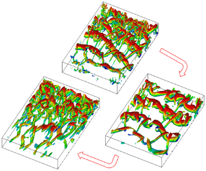
We study the energy exchange among TKE, MKE and MIE, and the compressibility effect on them in the transition region via both qualitative and quantitative analyses. Figures 5–7 show the contours of $\mathcal {P}$, $\varepsilon$, $\varPhi$, $\varPi$ and $\varPsi$ for $M_c = 0.3$, 0.5 and 0.7, respectively, with a break at $x = x_E$ separating the transition and turbulent regions. Since the initial velocity field is laminar (see part I for more detail), the normalized values of $\mathcal {P}$, $\varepsilon$, $\varPi$ and $\varPsi$ are relatively small at the beginning of the shear layer. In contrast, $\varPhi$ starts with a large value due to the considerable mean shear of two mean streams at the trailing edge of the splitter. As the shear layer develops, the flow instability increases; the turbulent production significantly outweighs the turbulent viscous dissipation, such that the kinetic energy grows. The extrema of $\mathcal {P}$, $\varepsilon$, $\varPi$ and $\varPsi$ shift to downstream, except $\varPhi$, which remains somewhat insensitive to the variation of the convective Mach number.

Figure 5. Contours of $\mathcal {P}$, $\varepsilon$, $\varPhi$, $\varPi$ and $\varPsi$ for $M_c = 0.3$ in the transition and turbulent regions separated by a vertical line at $x = x_E$. All terms are normalized by $({\rm \Delta} U)^3$.

Figure 6. Contours of $\mathcal {P}$, $\varepsilon$, $\varPhi$, $\varPi$ and $\varPsi$ for $M_c = 0.5$ in the transition and turbulent regions separated by a vertical line at $x = x_E$. All terms are normalized by $({\rm \Delta} U)^3$.

Figure 7. Contours of $\mathcal {P}$, $\varepsilon$, $\varPhi$, $\varPi$ and $\varPsi$ for $M_c = 0.7$ in the transition and turbulent regions separated by a vertical line at $x = x_E$. All terms are normalized by $({\rm \Delta} U)^3$.

The cross-stream profiles of $\mathcal {P}$, $\varepsilon$, $\varPhi$, $\varPi$ and $\varPsi$ are considered for the examination of the energy exchange and the compressibility effect on energy exchange. Figure 8 compares the normalized cross-stream profiles of the aforementioned five terms for $M_c = 0.3$, 0.5 and 0.7, respectively, at $x - x_R = 200$ near the middle of the laminar–turbulent region. Two peaks can be observed for $\varPsi$ over the cross-stream direction. One peak appears near the centre of the low-speed side of the shear layer, while another is approximately in the middle of the high-speed side. The centre of the shear layer becomes a valley and has the lowest value. These might be because the mean pressure gradients with respect to the cross-stream direction are larger at the edges of the high- and low-speed sides of the shear layer, and the magnitudes of $\langle v''\rangle$ are higher as well, compared with the centre of the shear layer. However, the mean pressure gradient with respect to the streamwise direction is insignificant, due to the nature of the compressible FSL flow, i.e. zero pressure gradient with respect to the flow direction. When the mean pressure gradient with respect to the cross-stream direction acts on the flow, the work done by the mean pressure gradient becomes a gain in the kinetic energy, resulting in two peaks along the cross-stream direction. The compressibility effect on the cross-stream variations of five budget terms is also demonstrated in figure 8. The peaks of the normalized $\mathcal {P}$, $\varepsilon$ and $\varPi$ decrease with increasing $M_c$, indicating that in the transition region, the normalized energy that transfers through $\mathcal {P}$, $\varepsilon$ and $\varPi$ decreases with increasing compressibility. However, the magnitudes of the normalized $\varPhi$ for all cases remain nearly constant with the change of $M_c$, suggesting that the normalized energy exchange through $\varPhi$ is almost unaffected by compressibility. With increasing $M_c$, the value of the normalized $\varPsi$ at the centre of the shear layer is unchanged, while the magnitudes of the two adjacent peaks increase, implying that the energy transferred through $\varPsi$ from TKE to MKE increases at the two sides of the shear layer.

Figure 8. Cross-stream variation of (a) $\mathcal {P}$, (b) $\varepsilon$, (c) $\varPhi$, (d) $\varPi$ and (e) $\varPsi$ for $M_c = 0.3$, 0.5, 0.7. All terms are extracted at $x - x_R = 200$ in transition region and normalized by $({\rm \Delta} U)^3/\delta _{\theta }$.

Figure 9(a) compares the magnitudes of the normalized $\mathcal {P}$, $\varepsilon$, $\varPhi$, $\varPi$ and $\varPsi$, at the lower edge ($y = -18.63$), centre ($y = y_{0.5}$) and upper edge ($y = 17.53$) along the cross-stream direction of the shear layer at $x_R = 200$ for $M_c = 0.3$. Here, $y_{0.5}$ is the lateral position at which the streamwise velocity reaches the convective velocity, $U_c$, in the cross-stream direction, where $U_c$ is defined as

(3.7)\begin{equation} U_c = \frac{U_1+U_2}{2}. \end{equation}

At the lower and upper edges of the shear layer, the magnitudes of all five terms are insignificant, while at the shear layer centre, the turbulent production and turbulent viscous dissipation terms have significant contributions to the energy exchange. Note that the ratio of $\mathcal {P}$ to $\varepsilon$ at the centre of the shear layer is approximately 3.5, meaning that in the transition region, the turbulent production considerably outweighs the turbulent viscous dissipation; hence the kinetic energy significantly grows. Figure 9(b) compares the magnitudes of the normalized $\mathcal {P}$, $\varepsilon$, $\varPhi$, $\varPi$ and $\varPsi$, for various $M_c$ at the centre of the shear layer. It is clearly shown that both the normalized $\mathcal {P}$ and $\varepsilon$ are significantly affected by compressibility; the normalized $\mathcal {P}$ and $\varepsilon$ decrease as $M_c$ increases. However, other terms appear nearly unchanged with various $M_c$, because of the adopted scale in the figure and their smaller contributions to the kinetic energy exchange, compared with that of $\mathcal {P}$ and $\varepsilon$.

Figure 9. Comparisons of $\mathcal {P}$, $\varepsilon$, $\varPhi$, $\varPi$ and $\varPsi$, (a) at the lower edge ($y = -18.63$), centre ($y = y_{0.5}$) and upper edge ($y = 17.53$) of the shear layer for $M_c = 0.3$, (b) at the centre of the shear layer for $M_c = 0.3$, 0.5 and 0.7, in transition region at $x-x_R = 200$. All terms are normalized by $({\rm \Delta} U)^3/\delta _{\theta }\times 10^{-4}$.

The influence of compressibility on energy exchange is further investigated by considering the evolution of the cross-stream integral, $\phi ^{I}$, which is defined as

(3.8)\begin{equation} \phi^{I} = \int_{-\infty}^{+\infty} \phi\, {\textrm{d} y} . \end{equation}

Here, $\phi$ represents any budget term that transfers energy among TKE, MKE and MIE. The superscript $I$ represents the cross-stream ($y$-line) integration. Since the aforementioned budget terms evolve in the streamwise direction and expand in the cross-stream direction, their cross-stream integral can provide information about their bulk behaviour and help to understand their energy exchange contributions along the streamwise direction.

Figure 10 presents the normalized $\mathcal {P}^{I}$, $\varepsilon ^{I}$, $\varPhi ^{I}$, $\varPi ^{I}$ and $\varPsi ^{I}$ as a function of $x-x_R$ in the transition region, for various $M_c$. As a result, we can compare the evolution of these budget terms for different Mach numbers with the same start locations of the turbulent transition region. Note that this streamwise evolution can only be observed in the spatially developing FSL but not in the temporally developing numerical simulations. The terms $\mathcal {P}^{I}$, $\varepsilon ^{I}$, $\varPi ^{I}$ and $\varPsi ^{I}$ start with a nearly zero magnitude, until perturbations grow, and their magnitudes increase. In contrast, $\varPhi ^{I}$ initiates with an extremum followed by a slow decline towards an asymptotic value. This means that the energy exchange from MKE to other forms of energy through $\varPhi ^{I}$ mainly occurs at the beginning of the shear flow. The evolutions of budget terms for different cases are significantly affected by the change of $M_c$, as observed in figure 10. The influence of compressibility for the normalized $\mathcal {P}^{I}$, $\varepsilon ^{I}$, $\varPi ^{I}$ and $\varPsi ^{I}$ becomes more significant as the flow advances downstream, but the normalized $\varPhi ^{I}$ remains nearly unchanged. The peaks of the normalized $\mathcal {P}^{I}$, $\varepsilon ^{I}$ and $\varPi ^{I}$ decrease as $M_c$ increases, while the peak of the normalized $\varPsi ^{I}$ increases. We can conclude that, in the transition region with increasing compressibility, the energy that transfers through $\mathcal {P}$, $\varepsilon$ and $\varPi$ decreases; energy exchange through $\varPhi$ is nearly unchanged; energy exchange through $\varPsi$ increases.

Figure 10. Evolution of the cross-stream integrals (a) $\mathcal {P}^{I}$, (b) $\varepsilon ^{I}$, (c) $\varPhi ^{I}$, (d) $\varPi ^{I}$ and (e) $\varPsi ^{I}$ for $M_c = 0.3$, 0.5 and 0.7 in the transition region. All terms are normalized by $({\rm \Delta} U)^3$.

We can observe a double-peak variation of $\mathcal {P}^{I}$ for $M_c = 0.3$ and 0.5 in figure 10(a). This phenomenon can be explained with the flow vortex structures. To inspect further, we present the corresponding enlarged area in figure 11(a). It can be seen that the magnitude of turbulent production rapidly rises at the position near the trailing edge, where the large structures dominate the flow. The value at the first peak ($x \approx 130$) is roughly 2.6 times that at $x \approx 1000$ in the self-similar region, while the second peak value is roughly $94\,\%$ of the first peak value. Note that the double peak spans from $x \approx 130$ to 240, which is within the transition area. To the best of our knowledge, this double-peak phenomenon has not been reported in the literature for planar free shear flows. We propose that two significant vortex pairings cause this kind of phenomenon.

Figure 11. (a) Evolution of $\mathcal {P}^{I}$ normalized by $({\rm \Delta} U)^3$, (b) spanwise vorticity contours and (c) isosurface of the second invariant of the velocity gradient tensor ($Q2 = 0.02$), coloured by streamwise velocity, for $M_c = 0.3$ in transition region.

We can relate the double-peak profile directly to the rise of the pairing vortex, based on the visualization of the flow structures presented in figure 11(b). Careful observation shows that the positions of the peaks, at $x \approx 130$ and 240, are in the same streamwise areas where the pairings occur, illustrated in the vorticity contours. This observation hints at the connection between the double peak and the behaviour of the vortex pairings. We further examine the evolution of the 3-D structures in the flow to understand how the vortex pairing leads to a peak of turbulent production. Figure 11(c) presents a 3-D representation of the turbulent structures via the isosurface of the second invariant of the velocity gradient tensor. From figure 11(c), the newly generated 2-D primary spanwise coherent structures near the trailing edge of the splitter form the first pairing at roughly $x = 130$. The first pairing generates a large vortex structure (which does not break into small vortices) (Ho & Huang Reference Ho and Huang1982; Moser & Rogers Reference Moser and Rogers1993). A large paired vortex structure maintains more kinetic energy than an unpaired roller vortex structure, and less dissipation than a paired vortex with broken-down structures (Sandham Reference Sandham1989). Therefore, the first peak of turbulent production occurs due to the appearance of the first pairing.

The large vortex structure formed by the first pairing continues rotating, twisting and stretching. As the intensity of the instability grows and reaches a triggering threshold level, the second pairing occurs and leads to the second peak of the turbulent production (Sandham Reference Sandham1989). At the same time, large vortex structures swirl into flower-shaped vortices, which start to play a dominant role in the breakdown of the mixing layer. The slender petals of the flower-shaped vortices develop with intense vorticity and break down into small vortices. These small vortices facilitate more dissipation and preserve less kinetic energy, making the second peak of turbulent production lower than the first peak. Subsequently, the flower-shaped vortices then evolve into hairpin vortices downstream, and more and more small vortices are generated near the centre of the hairpin vortices. The turbulent production gradually decreases as the flow advances downstream because the rate of turbulent viscous dissipation increases as the number of small vortices increases.

For the $M_c = 0.7$ case, only one peak appears in the profile of turbulent production, shown in figure 12(a). The single peak is because the 3-D secondary streamwise vortex structures become dominant in the roll-up region of the shear layer, which is demonstrated in figure 12(c) as well. The streamwise vortex structures then develop into lambda-shaped vortices (Sandham & Reynolds Reference Sandham and Reynolds1990, Reference Sandham and Reynolds1991; Lui & Lele Reference Lui and Lele2001; Fu & Li Reference Fu and Li2006; Zhou, He & Shen Reference Zhou, He and Shen2012; Zhang, Tan & Yao Reference Zhang, Tan and Yao2019), which are subjected to longitudinal elongation due to the high compressibility. These elongated vortex structures have less tendency to roll or pair in the streamwise direction (see figure 12b). The unpaired vortex structures directly evolve into hairpin vortices without experiencing rolling. The kinetic energy grows as the flow advances downstream. Prior to the point that the turbulent viscous dissipation becomes significant, the magnitude of turbulent production peaks. Next, small vortices dominate the flow, leading to a smooth decay of turbulent production.

Figure 12. (a) Evolution of $\mathcal {P}^{I}$ normalized by $({\rm \Delta} U)^3$, (b) spanwise vorticity contours and (c) isosurface of the second invariant of the velocity gradient tensor ($Q2 = 0.02$), coloured by streamwise velocity, for $M_c = 0.7$ in transition region.

3.2. Self-similar turbulence region

In this section, we investigate the evolutions of $\mathcal {P}$, $\varepsilon$, $\varPhi$, $\varPi$ and $\varPsi$, as well as the compressibility effects on them in the self-similar turbulent region. We compare the evolutions of the budget terms for different $M_c$ using a shifted streamwise axis, $x - x_E$. Consequently, we are able to examine the behaviours of the budget terms by eliminating the effect from the unequal laminar–turbulent transition lengths. Contours of the normalized $\mathcal {P}$, $\varepsilon$, $\varPhi$, $\varPi$ and $\varPsi$ for all cases are presented in figures 5–7. We can see that the start of the turbulent region significantly shifts to downstream with increasing $M_c$ (see part I for more details). As the flow advances downstream, $\mathcal {P}$, $\varepsilon$, $\varPhi$, $\varPi$ and $\varPsi$ decrease gradually, while expanding in the cross-stream direction, especially for $\mathcal {P}$, $\varepsilon$ and $\varPhi$, which grow linearly. This is attributed to the self-similarity nature of the FSL flow in the turbulent region.

In figures 13(a) and 13(b), we compare the cross-stream profiles of the normalized turbulent production and turbulent viscous dissipation from present simulations with the results by Rogers & Moser (Reference Rogers and Moser1994), generated from the DNS of a temporally evolving shear layer. Both results are extracted from the self-similar turbulent region for $M_c = 0.3$. The profiles from the present work noticeably shift to the low-speed side ($y < 0$) of the shear layer, compared with the result of Rogers & Moser (Reference Rogers and Moser1994). Despite the profiles shifting, the normalized values of turbulent production and dissipation are in agreement, confirming that the turbulent shear layer is correctly resolved. Note that the shear-layer bending is only captured in the spatially evolving turbulent shear layer simulations. We discuss the shear-layer bending in detail next.

Figure 13. Comparison of cross-stream profiles from the present work and the results by Rogers & Moser (Reference Rogers and Moser1994) for (a) turbulent production and (b) turbulent viscous dissipation at $x-x_E = 300$ in the self-similar turbulent region for $M_c = 0.3$. All terms are normalized by $({\rm \Delta} U)^3/\delta _{\theta }$.

To further investigate the shear-layer bending phenomenon, we start from the velocity isolines at the centre ($U_c$), upper-edge ($95\,\%U_1$) and lower-edge ($105\,\%U_2$) of the shear layer along the streamwise direction. As a result, the outline of the shear layer in the $x$–$y$ plane can be inspected. Figure 14(a) shows the velocity isolines of $95\,\%U_1$, $U_c$ and $105\,\% U_2$ for various $M_c$. We can see that as the convective Mach number increases, the growth rate of the shear layer decreases, resulting in a narrower shear layer contour. Moreover, the momentum thickness growth rates, $\textrm {d}\delta _{\theta }/{\textrm {d} x}$, in the turbulent region are computed as 0.0137, 0.0121 and 0.0106 for convective Mach numbers of 0.3, 0.5 and 0.7, respectively (see table 2). This trend confirms that the momentum thickness growth rate decreases as $M_c$ increases (Birch & Eggers Reference Birch and Eggers1972; Papamoschou & Roshko Reference Papamoschou and Roshko1988; Jackson & Grosch Reference Jackson and Grosch1989; Goebel & Dutton Reference Goebel and Dutton1991; Grosch & Jackson Reference Grosch and Jackson1991; Hall, Dimotakis & Rosemann Reference Hall, Dimotakis and Rosemann1993; Clemens & Mungal Reference Clemens and Mungal1995; Vreman, Sandham & Luo Reference Vreman, Sandham and Luo1996; Day, Reynolds & Mansour Reference Day, Reynolds and Mansour1998; Freund, Lele & Moin Reference Freund, Lele and Moin2000; Pantano & Sarkar Reference Pantano and Sarkar2002; Foysi & Sarkar Reference Foysi and Sarkar2010; Javed, Rajan & Chakraborty Reference Javed, Rajan and Chakraborty2013; Wang et al. Reference Wang, Wei, Zhang, Zhang and Xue2015). In figure 14(a), the $U_c$ contours are qualitatively similar for any given $M_c$, although there are some small differences in the contours in the transition region of the shear layer.

Figure 14. (a) Mean velocity isolines and (b) isolines of $U_c$ for various $M_c$, as a function of $x$.

A closer look at the $U_c$ contours helps to identify the compressibility effect on shear-layer bending, as shown in figure 14(b). The shift to the low-speed side starts from $x \approx x_R$. For a more explicit comparison, we normalize the streamwise axis as $x - x_R$ and add trendlines to all cases, shown in figure 15. The figure reveals that the centre of the shear layer extends further into the low-speed side as the convective Mach number increases (see figure 15b). This finding may help to explain the phenomenon in the backward-facing step (known as BFS) flow, where the reattachment length decreases as the inflow Mach number increases (Chen et al. Reference Chen, Yi, He, Tian and Zhu2012; Liu et al. Reference Liu, Wang, Guo, Zhang and Lin2013). This shifting of the mean velocity profile in the FSL has been reported in previous studies, both experimental and numerical (Elliott & Samimy Reference Elliott and Samimy1990; Goebel & Dutton Reference Goebel and Dutton1991; Fu & Li Reference Fu and Li2006). However, a detailed explanation of such behaviour is not available. In this work, we explain this behaviour quantitatively in terms of the asymmetry mass flux entrainment of the shear layer.

Figure 15. (a) Isolines of $U_c$ and (b) trendlines of the isolines for $M_c = 0.3$, 0.5 and 0.7, as a function of $x - x_R$.

In a plane FSL with different free stream speeds, the flow field can be classified into two regions: in one region the flow is primarily irrotational; in the another one the flow is mainly turbulent and rotational. Entrainment is the process that the mass flux traverses from the irrotational region into the rotational area (Corrsin & Kistler Reference Corrsin and Kistler1955). The mass flux entrainment ratio ($R_M$) is defined as the ratio of the fluid from the high-speed side to the fluid from the low-speed side into the shear layer. The mass flux entrainment ratio for an incompressible, plane FSL can be estimated by (Dimotakis Reference Dimotakis1986)

(3.9)\begin{equation} R_M = 1 + 3.9\frac{\delta_w}{x} , \end{equation}

where $\delta _w = {\rm \Delta} U/(\textrm {d}\lbrace u \rbrace / {\textrm {d} y})_{max}$ is the vorticity thickness. The empirical constant 3.9 was suggested by Koochesfahani et al. (Reference Koochesfahani, Catherasoo, Dimotakis, Gharib and Lang1979). Dimotakis (Reference Dimotakis1986) also proposed a simplified equation to determine the mass flux entrainment ratio in the turbulent region of the shear layer, i.e.

(3.10)\begin{equation} R_M = 1 + 0.68R , \end{equation}

where $R$ is the velocity ratio defined by (2.13). The results calculated by (3.9) and (3.10) are plotted in figure 16(a) as a function of $x$ for $M_c = 0.3$. We can see that the result estimated by (3.9) starts with a relatively low value of $1.2$ at $x \approx 100$. As advancing downstream, the magnitude gradually increases and overtakes the result calculated by (3.10) at $x \approx 200$ in the transition region. It means that the entrainment ratio in the transition region is slightly higher than that in the turbulent region. There are two different entrainment mechanisms in turbulent FSL flow, namely, entrainment by engulfment in the transition region and by nibbling in the turbulent area (Mathew & Basu Reference Mathew and Basu2002; Jahanbakhshi & Madnia Reference Jahanbakhshi and Madnia2016). The results of figure 16(a) indicate that compared with entrainment by nibbling, entrainment by engulfment may yield higher mass entrainment ratio. After the $R_M$ estimated by (3.9) reaches a maximum at $x \approx 350$, where the flow turns into turbulence, the magnitude of $R_M$ by (3.9) gradually matches with the asymptotic value estimated by (3.10). In the turbulent area, the entrainment ratio is relatively steady, and the mass, momentum and energy are mainly entrained by nibbling. The mass flux entrainment from the high-speed side is significantly more than that from the low-speed side, leading to the momentum difference across the shear layer in the cross-stream direction, therefore causing the bending.

Figure 16. (a) Mass flux entrainment ratios estimated by (3.9) and (3.10) for $M_c = 0.3$ and (b) shear layer and bending angle schematic.

We have concluded that the asymmetric entrainment leads to the shear-layer bending. In this context, we further investigate this bending by the estimation of the bending angle. Dimotakis (Reference Dimotakis1986) proposed a method to estimate the angle between the upper edge and the $x$-axis of the shear layer, indicated by $\alpha _1$, and the angle between the lower edge and the $x$-axis, denoted by $\alpha _2$. The corresponding angles are also demonstrated in figure 16(b). Angles $\alpha _1$ and $\alpha _2$ can be estimated by (Dimotakis Reference Dimotakis1986)

(3.11)\begin{gather} \frac {1+R}{1-R} \left( \frac{\tan \alpha_1}{\tan \alpha_2 + \tan \beta }\right) = R_M , \end{gather}

(3.12)\begin{gather}\tan \alpha_1 + \tan \alpha_2 = \frac{\textrm{d}\delta_{vis}}{\textrm{d} x} , \end{gather}

where $\tan \beta = V_2/U_2$ and $V_2$ is the cross-stream component of the low-speed mean velocity at the shear layer edge. Here $\delta _{vis}$ is the visual thickness and has been suggested to be approximately two times the vorticity thickness $\delta _{w}$ (Brown & Roshko Reference Brown and Roshko1974). Thus, (3.12) can be modified as

(3.13)\begin{equation} \frac{1}{2}(\tan \alpha_1 + \tan \alpha_2) = \frac{\textrm{d}\delta_{w}}{\textrm{d} x} . \end{equation}

After obtaining angles $\alpha _1$ and $\alpha _2$, the bending angle $\alpha$ can be calculated by

(3.14)\begin{equation} \alpha = \frac{1}{2}(\alpha_2 - \alpha_1) . \end{equation}

Conversely, using the current results shown in figure 14(a), we can estimate the angles $\alpha _1$ and $\alpha _2$, which can be used to calculate $\alpha$ and $R_M$ by employing (3.14) and (3.11), respectively, for different $M_c$. The results are tabulated in table 3. Through data fitting, the data in table 3 can be used to modify (3.10) for the $R_M$ estimation of the compressible planar FSL flow, i.e.

(3.15)\begin{equation} R_M = 1+0.46R+0.18M_c+0.08M_c^2 , \end{equation}

for $M_c \leqslant 0.7$, due to the limited convective Mach numbers used in this work. Furthermore, we can use the angles in table 3 to verify (3.13). The vorticity thickness growth rates are calculated as 0.058, 0.055 and 0.051 for $M_c = 0.3$, 0.5 and 0.7, respectively, from (3.13). The computed results have excellent agreements with the corresponding results, 0.060, 0.055 and 0.050, estimated by $\textrm {d}\delta _w/{\textrm {d} x}$ with $\delta _w = {\rm \Delta} U/(\textrm {d}\lbrace u \rbrace / {\textrm {d}y})_{max}$. This confirms that, for the conditions considered in this study, (3.13) can accurately predict the relation between angles $\alpha _1$ and $\alpha _2$ with the vorticity growth rate.

Table 3. Shear-layer bending angles in degrees for $M_c = 0.3$, 0.5 and 0.7.

Figure 17. Cross-stream profiles of the normalized (a) turbulent convection and (b) turbulent transport at $x - x_E = 300$ in the turbulent region for $M_c = 0.3$. All terms are normalized by $({\rm \Delta} U)^3/\delta _{\theta }$.

Figure 18. Cross-stream profiles of the streamwise Favre-averaged velocity at five streamwise locations for (a) $M_c = 0.3$ and (b) $M_c = 0.7$.

The asymmetric entrainment in the turbulent region is also reflected from the cross-stream profiles of kinetic energy budget terms, such as kinetic energy convection and transport terms. Brown & Roshko (Reference Brown and Roshko1974) proposed that entrainment is composed of three mechanisms: mean velocity engulfment, turbulent convection and turbulent transport; and the entrainment includes mass, momentum and energy entrainment. In the transition regions, the engulfment is the dominant mechanism for entrainment. In contrast, the turbulent convection and transport are the leading mechanisms in the turbulent region (Brown & Roshko Reference Brown and Roshko1974). The turbulent convection ($TC$), $\partial \langle \rho \rangle \{u_k\}\{k\} / \partial x_k$, is the first term of (3.1), while the turbulent transport ($TT$) is

(3.16)\begin{equation} TT = -\frac{\partial \langle\rho\rangle\{u_k''k''\}}{\partial x_k} - \frac{\partial \langle p'u_k'\rangle}{\partial x_k} + \frac{\partial \langle\tau_{ik}' u_i'\rangle}{\partial x_k} , \end{equation}

where $\partial \langle \rho \rangle \{u_k''k''\} / \partial x_k$, $\partial \langle p'u_k'\rangle / \partial x_k$ and $-\partial \langle \tau _{ik}' u_i'\rangle / \partial x_k$ are the second, third and fourth terms on the RHS of (3.1). Turbulent convection and transport play crucial roles in the lateral and longitudinal transport of mass, momentum and energy. Figures 17(a) and 17(b) show the cross-stream profiles of the turbulent convection and transport at $x - x_E = 300$ in the turbulent region for $Mc = 0.3$. The kinetic energy from the free streams entrains into the shear layer often through two regions. One region is laterally above the centre of the shear layer, between the high-speed free stream and the upper shear layer; another region is laterally below the shear layer, between the low-speed free stream and the lower shear layer. Both turbulent convection and turbulent transport profiles are double peaked, and the peaks are located in the two regions mentioned above. Note that the gain of the kinetic energy by convection and transport from the high-speed side outweighs that from the low-speed side. This again demonstrates the asymmetric entrainment from the edges of the shear layer.

It is worth noting that, in figure 14(b), in the region $x < 150$, the lateral position of $U_c$ locates at $y \approx 2.5$, rather than $y \approx 0$. This higher position is due to the rise of the velocity deficit. In the experiment, boundary layers develop along two sides of the splitter plate, then meet at the trailing edge, resulting in a velocity deficit. In this work, the velocity deficit in the shear layer follows two laminar boundary layers along the two sides of the splitter. In other words, two laminar boundary layers meet at the trailing edge while maintaining their laminar flow behaviours due to the inertia of the fluid. As a result, a layer of fluid with near-zero velocity (stagnation area) is formed downstream of the trailing edge. The cross-stream Favre-averaged velocity profiles of the shear layer are presented in figure 18 for five selected locations. We can see how the confluence initially results in a velocity deficit that decreases in the streamwise direction. The flow eventually evolves into a self-similar shear layer.

For the case with $M_c = 0.3$ in figure 18(a), the velocity deficit is observable up to $x = 131.5$ downstream of the trailing edge, beyond which the flow displays the features of a classical FSL. An estimate of the velocity deficit magnitude with downstream distance is shown in table 4. The velocity deficit, $U_d$, is calculated as

(3.17)\begin{equation} U_d = \left( U_{{erf}}\right)_{c} - \lbrace u \rbrace_{min} , \end{equation}

where $( U_{{erf}})_{c}$ is the velocity at the centre ($y = y_{0.5}$) of the classical error function profile, and $\lbrace u \rbrace _{min}$ is the minimum velocity of the cross-stream profile of the streamwise Favre-averaged velocity from the current study. The classical error function profile was derived by Gortler (Reference Gortler1942), assuming constant viscosity and density across the shear layer, defined as

(3.18)\begin{equation} U_{{erf}} = U_2 + \frac{{{\rm \Delta} U}}{2}[1+\text{erf}(\eta)] . \end{equation}

Here, $\eta$ is the similarity variable, expressed as

(3.19)\begin{equation} \eta = \frac{(y - y_{0.5})}{(x - x_0)} , \end{equation}

where $x_0$ is the origin of the FSL. The data in table 4 can be extrapolated to predict that the velocity deficit should disappear approximately at $x = 132$ after the confluence, also demonstrated in figure 19(a). Similarly, we calculate the velocity deficit for $M_c = 0.7$, shown in figure 18(b) and tabulated in table 5. Again, we can predict that the classic shear-layer profile can be recovered approximately at $x = 428$, presented in figure 19(b) as well. For convenience, we call the distance between the initial emergence and the final disappearance of the velocity deficit the VDPD. Furthermore, based on the trend observed in figure 19, we can deduce that the VDPD increases as the convective Mach number increases.

Table 4. Velocity deficit with downstream distance for $M_c = 0.3$.

Figure 19. Evolution of the velocity deficit along the streamwise direction for (a) $M_c = 0.3$ and (b) $M_c = 0.7$. The red dashed line is the added trendline for each case.

Table 5. Velocity deficit with downstream distance for $M_c = 0.7$.

To examine the energy contributions of budget terms in the cross-stream direction, we compare the normalized $\mathcal {P}$, $\varepsilon$, $\varPhi$, $\varPi$ and $\varPsi$ at the lower edge ($y = -62.45$), centre and upper edge ($y = 41.47$) of the shear layer at $x - x_E = 300$ in the turbulent region, shown in figure 20(a). At the lower and upper edges of the shear layer, the magnitudes of all normalized terms are near zero, while at the shear layer centre, the turbulent production and turbulent viscous dissipation have considerable contributions to the energy exchange. Note that the ratio of $\mathcal {P}$ to $\varepsilon$ at the centre of the shear layer is approximately 1.3. This near unity ratio indicates that in the turbulent region, the energy contribution of the turbulent viscous dissipation almost overtakes that of the turbulent production; hence the growth rate of the kinetic energy gradually decreases. Figure 20(b) compares the magnitudes of the five normalized terms for different $M_c$ at the centre of the shear layer. We can see that the normalized $\mathcal {P}$ and $\varepsilon$ significantly decrease with increasing $M_c$, whereas the other terms show only small changes, due to the employed scale and their relatively small energy contributions.

Figure 20. Comparisons of $\mathcal {P}$, $\varepsilon$, $\varPhi$, $\varPi$ and $\varPsi$, (a) at the lower edge ($y = -62.45$), centre and upper edge ($y = 41.47$) of the shear layer for $M_c = 0.3$, (b) at the centre of the shear layer for $M_c = 0.3$, 0.5 and 0.7, at $x - x_E = 300$ in turbulent region. All terms are normalized by $({\rm \Delta} U)^3/\delta _{\theta }\times 10^{-4}$.

The evolutions of the normalized $\mathcal {P}^{I}$, $\varepsilon ^{I}$, $\varPhi ^{I}$, $\varPi ^{I}$ and $\varPsi ^{I}$ in the turbulent region are shown in figure 21. The magnitudes of the five normalized terms decay gradually to asymptotic values, due to the turbulent viscous dissipation and the shear layer cross-stream diffusion. With increasing $M_c$, the normalized $\mathcal {P}^{I}$ and $\varepsilon ^{I}$ decrease, as shown in figures 21(a) and 21(b), due to the reductions of Reynolds stresses and velocity fluctuations, respectively. In the turbulent region, the value of $\varPhi ^{I}$ becomes very small (see figure 21c), meaning that most large vortex structures have turned into small vortex structures. Also, the value of $\varPhi ^{I}$ is not significantly affected by compressibility. This is attributed to the insensitive mean velocity field with respect to the change of $M_c$. In contrast, the normalized value of $\varPsi ^{I}$ increases with increasing $M_c$ (see figure 21e), owing to the sensitive cross-stream pressure gradient with respect to compressibility. Figure 21(d) shows that the normalized value of $\varPi ^{I}$ decreases significantly from $M_c = 0.3$ to 0.5, while remains almost the same from $M_c = 0.5$ to 0.7. As the flow advances downstream, the magnitudes of the normalized $\varPi ^{I}$ for all cases become very close to zero, suggesting that the contribution of the pressure dilatation to the TKE is insignificant. This is attributed to the self-cancellation of temporal oscillations when averaging the instantaneous pressure dilatation, $p'(\partial {u_k'}/{\partial x_k})$ over time. Thus, we examine the importance of $p'(\partial {u_k'}/\partial {x_k})$, instead.

Figure 21. Evolution of the cross-stream integrals (a) $\mathcal {P}^{I}$, (b) $\varepsilon ^{I}$, (c) $\varPhi ^{I}$, (d) $\varPi ^{I}$ and (e) $\varPsi ^{I}$ for $M_c = 0.3$, 0.5 and 0.7 in turbulent region. All terms are normalized by $({\rm \Delta} U)^3$.

The evolution of $p'(\partial {u_k'}/\partial {x_k})$ at a typical location $(x - x_E, y, z) = (300, -6.5, 40)$ is presented as a function of flow-through-time and compared with the budget term turbulent production, shown in figure 22. The flow-through-time is defined as the time required for the flow to travel from the inlet to the outlet with the convective velocity, i.e.

(3.20)\begin{equation} \text{flow-through-time} = \frac{L_x}{U_c} . \end{equation}

From figure 22, we can see that $p'(\partial {u_k'}/\partial {x_k})$ develops oscillations in time with relatively large amplitudes; its negative and positive extrema are nearly symmetric; the magnitude of its extremum increases from $1.08\times 10^{-4}$ to $1.47\times 10^{-4}$ and $3.11\times 10^{-4}$ as $M_c$ increases from 0.3 to 0.5 and 0.7. The fluctuations of the pressure dilatation are also comparable to the value of turbulent production. Thus, the fluctuations of pressure dilatation have a significant contribution to the evolution of TKE, and increase in magnitude with increasing $M_c$.

Figure 22. Evolution of the instantaneous pressure dilatation (known as IPD) and the turbulent production at $x - x_E = 300$, $y = -6.5$ and $z = 40$ in the self-similar turbulent region, normalized by $({\rm \Delta} U)^3/\delta _{\theta }$.

The effect of compressibility on the fluctuations of pressure dilatation is also evidenced by a marked difference in the probability density functions (p.d.f.s) of the normalized instantaneous pressure dilatation. The p.d.f.s at $x - x_E = 300$, $y = -6.5$ and $z = 40$ in the self-similar turbulent region for cases with $M_c = 0.3$, 0.5 and 0.7 are presented in figure 23. In all cases, the expected exponential roll-off of the p.d.f. is obvious. However, the p.d.f. from the high convective Mach number case is slightly less symmetric about zero. The right- and left-hand tails of the p.d.f. become longer with increasing convective Mach number, suggesting that the range of the pressure-dilatation fluctuations increases monotonically with $M_c$, which is consistent with the conclusion from figure 22. Note that the increased range of fluctuations is smaller as $M_c$ increases from 0.5 to 0.7, compared with that from 0.3 to 0.5. Moreover, the peak of the p.d.f. at zero is more pronounced in the low convective Mach number cases, implying that more small values of pressure-dilatation fluctuations are present in such cases. The impact of compressibility on turbulent production and dissipation terms are further examined in the next section by analysing their components.

Figure 23. Probability density functions of instantaneous pressure dilatation at $x - x_E = 300$, $y = -6.5$ and $z = 40$ in the self-similar turbulent region, normalized by $({\rm \Delta} U)^3/\delta _{\theta }$.

Figure 24. Cross-stream profiles of the normalized turbulent production and its significant components for (a) $M_c = 0.3$, (b) $M_c = 0.5$ and (c) $M_c = 0.7$ at $x - x_E = 300$ in the turbulent region and normalized by $({\rm \Delta} U)^3/\delta _{\theta }$.

Figure 25. Comparison of the normalized $\{u''v''\}$ profiles at $x - x_E = 300$ in turbulent region for different convective Mach numbers.

3.3. Components of turbulent production and viscous dissipation

The previous section shows that the turbulent production and viscous dissipation make the most significant contributions to the energy exchange among TKE, MKE and MIE. To further investigate the compressibility effects on the energy exchange in the shear layer, we decompose these terms and analyse their components and the compressibility effects on them. The turbulent production term can be decomposed into

(3.21)\begin{align} \mathcal{P} &= -\langle\rho\rangle\{u''u''\} \frac{\partial \{u\}}{\partial x} -\langle\rho\rangle\{v''v''\} \frac{\partial \{v\}}{\partial y} -\langle\rho\rangle\{w''w''\} \frac{\partial \{w\}}{\partial z} -\langle\rho\rangle\{u''v''\} \frac{\partial \{u\}}{\partial y} \nonumber\\ &\quad -\langle\rho\rangle\{u''w''\} \frac{\partial \{u\}}{\partial z} -\langle\rho\rangle\{v''u''\} \frac{\partial \{v\}}{\partial x} -\langle\rho\rangle\{v''w''\} \frac{\partial \{v\}}{\partial z} -\langle\rho\rangle\{w''u''\} \frac{\partial \{w\}}{\partial x} \nonumber\\ &\quad -\langle\rho\rangle\{w''v''\} \frac{\partial \{w\}}{\partial y}. \end{align}

Here, the third, fifth, seventh, eighth and ninth terms on the RHS of (3.21) are negligible since the current shear layer is statistically homogeneous in the spanwise direction. Consequently, the expression for turbulent production can be reduced to

(3.22)\begin{equation} \mathcal{P} \approx \underbrace{-\langle\rho\rangle\{u''u''\} \frac{\partial \{u\}}{\partial x}}_{\mathcal{P}_1 } \underbrace{-\langle\rho\rangle\{v''v''\} \frac{\partial \{v\}}{\partial y}}_{\mathcal{P}_2 } \underbrace{-\langle\rho\rangle\{u''v''\} \frac{\partial \{u\}}{\partial y}}_{\mathcal{P}_3 } \underbrace{-\langle\rho\rangle\{v''u''\} \frac{\partial \{v\}}{\partial x}}_{\mathcal{P}_4 }. \end{equation}

For brevity, $-\langle \rho \rangle \{u''u''\} {\partial \{u\}}/{\partial x}$, $-\langle \rho \rangle \{v''v''\} {\partial \{v\}}/{\partial y}$, $-\langle \rho \rangle \{u''v''\} {\partial \{u\}}/{\partial y}$ and $-\langle \rho \rangle \{v''u''\} {\partial \{v\}}/{\partial x}$ are referred to as $\mathcal {P}_1$, $\mathcal {P}_2$, $\mathcal {P}_3$ and $\mathcal {P}_4$, respectively. The cross-stream variations of these terms are shown in figure 24 for various $M_c$. The dominant component in the turbulent production equation, (3.22), is $\mathcal {P}_3$, indicating that the planar FSL behaves statistically as a 2-D flow, as shown in the previous studies. Thus, as $M_c$ increases, the decrease of the normalized turbulent production is attributed to the reduction of $\mathcal {P}_3$. On the other hand, the normalized $\{u\}$ is not considerably affected by compressibility. Hence, the reduction of $\mathcal {P}_3$ is mainly due to the reduction of $\{u''v''\}$, which is demonstrated in figure 25. Vreman et al. (Reference Vreman, Sandham and Luo1996) showed that the growth rate of a temporal mixing layer is proportional to the integrated turbulence production component, $\mathcal {P}_3^{I}$, in the fully developed turbulent region. In a temporally evolving plane FSL, such relation can be expressed as (Vreman et al. Reference Vreman, Sandham and Luo1996)

(3.23)\begin{equation} \frac{\textrm{d}\delta_\theta}{\textrm{d}t} = -\frac{2}{\rho_o({\rm \Delta} U)^2} \int_{-\infty}^{+\infty} \langle\rho\rangle\{u''v''\} \frac{\partial \{u\}}{\partial y} {\textrm{d} y} . \end{equation}

Combining (3.8) with (3.23), the relation between the temporal growth rate and turbulent production is further simplified to

(3.24)\begin{equation} \frac{\textrm{d}\delta_\theta}{\textrm{d}t} = \frac{2 \mathcal{P}_3^{I}}{\rho_o({\rm \Delta} U)^2} . \end{equation}

The relation between the momentum thickness growth rates of temporally and spatially developing FSLs can be expressed as (Brown & Roshko Reference Brown and Roshko1974)

(3.25)\begin{equation} \frac{\textrm{d}\delta_\theta}{\textrm{d}t} = \frac{{\rm \Delta} U}{2R}\frac{\textrm{d}\delta_\theta}{\textrm{d} x} . \end{equation}

Then, the corresponding momentum thickness growth rate of a spatially developing FSL in the turbulent region becomes

(3.26)\begin{equation} \frac{\textrm{d}\delta_\theta}{\textrm{d} x} = \frac{4R \mathcal{P}_3^{I}}{\rho_o({\rm \Delta} U)^3} . \end{equation}

It is clear that the growth rate of a spatial FSL is proportional to the integrated turbulence production component, $\mathcal {P}_3^{I}$, and the growth rate can be calculated from (3.26). At $x - x_E =300$ in the turbulent region, the normalized integral of turbulent production is $\mathcal {P}_3^{I}/({\rm \Delta} U)^3 = 0.00641$, 0.00581 and 0.00495 for $M_c = 0.3$, 0.5 and 0.7, respectively. Consequently, the momentum thickness growth rates are $d\delta _\theta /{\textrm {d} x} = 0.0138$, 0.0125 and 0.0107 by employing (3.26). These results have excellent agreements with the corresponding results, $\textrm {d}\delta _\theta /{\textrm {d} x} = 0.0137$, 0.0121 and 0.0106, listed in table 2 computed using (2.17). This suggests that, for the conditions considered in this study, temporal simulation is capable of predicting the compressible FSL growth rate, despite the fact that temporal simulation possesses some significant drawbacks for simulating turbulent FSL, such as the lack of ability in capturing the effects of the velocity ratio across the FSL and the asymmetry of entrainment (Ho & Huerre Reference Ho and Huerre1984; Hussaini & Voigt Reference Hussaini and Voigt1990; Lui & Lele Reference Lui and Lele2001; Pickett & Ghandhi Reference Pickett and Ghandhi2002; Fu & Li Reference Fu and Li2006).

Besides the dominant component $\mathcal {P}_3$, the component $\mathcal {P}_1$ shows noticeable variations across the shear layer in figure 24. The value of $\mathcal {P}_1$ is negative in the low-speed side of the shear layer and slightly positive in the high-speed side. Note that $\{u''u''\}$ is always positive, thus, does not affect the sign of $\mathcal {P}_1$. The sign of $\mathcal {P}_1$ is determined by $\partial \{u\}/\partial x$. Note that a negative value of $\partial \{u\}/\partial x$ means a compression in the streamwise direction while a positive value does the opposite. Consequently, fluid elements in the low- and high-speed sides experience compression and expansion, respectively. This is a further evidence of the commonly recognized phenomenon that the mixing layer bends towards the side with lower speed. Furthermore, the value of $\mathcal {P}_1$ is almost unaffected by the change of $M_c$. As mentioned above, $\{u\}$ is nearly not influenced by compressibility. Based on the result from part I, $\{u''u''\}$ is not sensitive to the change of $M_c$ either. Therefore, $\mathcal {P}_1$ is not a function of $M_c$.

The compressibility effect on the turbulent viscous dissipation term is also further investigated by considering its components (Huang et al. Reference Huang, Coleman and Bradshaw1995),

(3.27)\begin{equation} \varepsilon\equiv\left\langle\tau_{ik}'\frac{\partial u_i'}{\partial x_k} \right\rangle = \varepsilon_1+\varepsilon_2+\varepsilon_3, \end{equation}

where

(3.28)\begin{gather} \varepsilon_1 = \langle\mu\rangle\left\langle\frac{\partial u_i'}{\partial x_k} \left(\frac{\partial u_i'}{\partial x_k} +\frac{\partial u_k'}{\partial x_i}\right)\right\rangle -\frac{2}{3}\langle\mu\rangle\left\langle\frac{\partial u_i'}{\partial x_k}\frac{\partial u_l'}{\partial x_l} \right\rangle\delta_{ik}, \end{gather}

(3.29)\begin{gather}\varepsilon_2 = \left\langle\mu'\frac{\partial u_i'}{\partial x_k} \left(\frac{\partial u_i'}{\partial x_k} +\frac{\partial u_k'}{\partial x_i}\right)\right\rangle -\frac{2}{3}\left\langle\mu'\frac{\partial u_i'}{\partial x_k}\frac{\partial u_l'}{\partial x_l} \right\rangle\delta_{ik}, \end{gather}

(3.30)\begin{gather}\varepsilon_3 = \left\langle\mu'\frac{\partial u_i'}{\partial x_k}\right\rangle \left(\frac{\partial \langle u_i\rangle}{\partial x_k} +\frac{\partial \langle u_k\rangle}{\partial x_i}\right) -\frac{2}{3}\left\langle\mu'\frac{\partial u_i'}{\partial x_k}\right\rangle \frac{\partial \langle u_l\rangle}{\partial x_l}\delta_{ik}. \end{gather}

When fluctuations in viscosity are neglected, only $\varepsilon _1$ is significant. This term can be decomposed into solenoidal dissipation, $\varepsilon _s$, dilatational dissipation, $\varepsilon _d$, and inhomogeneous dissipation, $\varepsilon _I$,

(3.31)\begin{equation} \varepsilon \approx \varepsilon_1=\varepsilon_s+\varepsilon_d+\varepsilon_I, \end{equation}

where

(3.32)\begin{gather} \varepsilon_s = 2\langle \mu \rangle \langle\omega_{ij}'\omega_{ij}'\rangle, \end{gather}

(3.33)\begin{gather}\varepsilon_d = \frac{4}{3} \langle \mu \rangle \left\langle\frac{\partial u_l'}{\partial x_l}\frac{\partial u_k'}{\partial x_k} \right\rangle, \end{gather}

(3.34)\begin{gather}\varepsilon_I = 2 \langle \mu \rangle \left(\frac{\partial ^2\langle u_i'u_j'\rangle}{\partial x_i\partial x_j} -2\frac{\partial }{\partial x_i}\left\langle u_i'\frac{\partial u_j'}{\partial x_j}\right\rangle\right), \end{gather}

with

(3.35)\begin{equation} \omega_{ij}'=\frac{1}{2}\left(\frac{\partial u_i'}{\partial x_j} -\frac{\partial u_j'}{\partial x_i}\right). \end{equation}

Figures 26(a) and 26(b) show the normalized cross-stream profiles of the solenoidal dissipation and the dilatational dissipation, respectively, as a function of $y/\delta _\theta$ at $x - x_E = 300$ in the turbulent region for all three cases. The magnitude of the normalized solenoidal dissipation decreases with increasing $M_c$, while the normalized dilatational dissipation shows the opposite trend. Figure 26(c) presents the ratio of the dilatational dissipation to the solenoidal dissipation in the same location, which reveals the following findings: the dilatational dissipation is approximately three orders of magnitude smaller than the solenoidal dissipation for $M_c = 0.5$ and 0.7; for $M_c = 0.3$, the magnitude of the dilatational dissipation is nearly four orders of magnitude smaller than that of the solenoidal dissipation; the ratio of the dilatational dissipation to the solenoidal dissipation increases as the $M_c$ increases. For the convective Mach numbers used in the present study, the dilatational dissipation seems to play an insignificant role in the TKE budget. This conclusion is consistent with the temporal simulation results by Blaisdell & Zeman (Reference Blaisdell, Zeman, Moin, Reynolds and Kim1992) and Vreman et al. (Reference Vreman, Sandham and Luo1996). The inhomogeneous dissipation component results from the shear between the shear layer (parallel to the wall) and the wall (Lele Reference Lele1994; Huang et al. Reference Huang, Coleman and Bradshaw1995; Cadiou, Hanjalic & Stawiarski Reference Cadiou, Hanjalic and Stawiarski2004; Brown et al. Reference Brown, Shaver, Lahey and Bolotnov2017). Thus, inhomogeneous dissipation approaches zero when far away from the wall. As expected, the inhomogeneous dissipation term is near zero in the turbulent region based on the current DNS results. Therefore, the inhomogeneous dissipation has insignificant contribution to the energy exchange between TKE and MIE.

Figure 26. Cross-stream profiles of (a) normalized solenoidal dissipation, $\varepsilon _{s}/(({\rm \Delta} U)^3/\delta _{\theta })$, (b) normalized dilatational dissipation, $\varepsilon _{d}/(({\rm \Delta} U)^3/\delta _{\theta })$. (c) Ratios of dilatational dissipation to solenoidal dissipation, $\varepsilon _{d}/\varepsilon _{s}$, as a function of $y/\delta _\theta$ at $x - x_E = 300$.