2. The LC Model and Extensions

The LC model defines the force of mortality as

(1) $$\log \left( {u_{x,t} } \right) = a_x + b_x k_t $$

where u _x,t is the force of mortality at age x in year t, a _x is the average log mortality at age x measured over the period in which the model is fit, b _x is the rate of change of the log mortality with time at age x and k _t is the time index for calendar year t. This model cannot be fit with the Generalised Linear Model (GLM) framework due to the multiplicative nature of the second term b _xk _t, which is comprised of two (latent) variables that must each be estimated from the data. Thus, two alternative approaches to fit the LC model have been developed. The original approach (Lee & Carter Reference Lee and Carter1992) is to apply a SVD to the matrix of log mortality rates, centred by subtracting the average log mortality at each age from each row of the matrix. The first left and right vectors from the SVD provide values for b _x and k _t. A second approach (Brouhns et al. Reference Brouhns, Denuit and Vermunt2002) (illustrated in more detail in Currie (Reference Currie2016)) is to specify the LC model as a statistical model (on the assumption that log mortality rates are normally distributed, see also Remark 2.1). More specifically, a Generalised Non-linear Model (GNM) is used (see Turner & Firth (Reference Turner and Firth2007)), and then maximum likelihood method is applied to fit the model. The LC model is generally fit to historical mortality data, and the time index coefficients k _t are then forecast using a standard time series model to produce forecasts of future mortality rates.

Remark 2.1. The specification in (1) aims to model mortality rates directly. Another approach is to use Poisson rate regression to model counts of deaths, using the central exposed to risk as the exposure. For simplicity, we focus on the first case in this research, but note that our approach carries over to the case of Poisson rate regression.

Extending the LC model to multiple populations generally involves adding terms to (1) that refer to some combination of the pooled mortality of the entire population and the specific mortality of each individual population. For example, Li & Lee (Reference Li and Lee2005) model mortality as

(2)$$\log \left( {u_{x,t} } \right) = a_x^i + b_x k_t + b_x^i k_t^i $$

where $$b_x^i $$ and $$k_t^i $$ are the rate of change of the log mortality with time and the time index, respectively, both for population i, which could, for example, refer to males and females in the same country, or populations from different countries. Li & Lee (Reference Li and Lee2005) refer to this model as the Augmented Common Factor (ACF) model, which is fit in three steps – firstly, the population-specific average mortality $$a_x^i $$ is calculated and subtracted from the matrix of mortality rates; secondly, the change with time of the pooled population mortality b _xk _t is estimated; and, finally, the change with time of the residual population-specific mortality $$b_x^i k_t^i $$ is estimated from the residual matrix $$ \mu _{x,t} - a_x^i - b_x k_t $$.

A variation of this model is the CAE model of Kleinow (Reference Kleinow2015), which we define in a simplified manner as follows:

(3)$$\log \left( {u_{x,t} } \right) = a_x^i + b_x k_t^i $$

where the rate of change of the log mortality with time is pooled (the “CAE”), but the time index is population specific. This model was fit in Kleinow (Reference Kleinow2015) using Common Principal Components and in Enchev et al. (Reference Enchev, Kleinow and Cairns2017) using maximum likelihood techniques.

More terms relating to the change of the log mortality with time could be added to any of the models (1), (2) or (3). For example, the full CAE model presented in Kleinow (Reference Kleinow2015) is

$$\log \left( {u_{x,t} } \right) = a_x^i + b(1)_x k(1)_t^i + b(2)_x k(2)_t^i $$

where terms in parentheses indicate that, for example, b(1)_x is the first change of mortality component, and so on. Another variation is the two-tier ACF model of Chen & Millossovich (Reference Chen and Millossovich2018), who include both gender-specific and gender- and population-specific terms in their model. Also, the specifications of the ACF and CAE models could be combined by including common factors and common effects within the same model.

Thus, the LC model can be extended using several different model specifications, but, to date, no theory has emerged explaining why these specifications may be more or less optimal for a particular set of mortality rates (though, some partial explanation is found in Villegas et al. (Reference Villegas, Haberman, Kaishev and Millossovich2017)). Therefore, we conclude that the specification of extended LC models appears somewhat arbitrary and depends on the judgment of the modeller, leading us to automate this process in the next section. Also, the extended LC models are not flexible enough to fit mortality data that are dissimilar from each other; thus, Li & Lee (Reference Li and Lee2005) and Kleinow (Reference Kleinow2015) are forced to choose mortality data from regions that, a priori, would seem to have similar mortality experience. On the other hand, we aim to design a model with sufficient flexibility to model all mortality rates in the HMD since 1950 simultaneously, and turn specifically to neural networks, which have a sufficiently high representational capacity for this task.

3. Representation Learning and Neural Networks

We approach the extension of the LC model in (1) from two perspectives. Firstly, the LC model can be seen as a regression model, where mortality rates (the target or dependent variable) are predicted using features (independent variables) that, in the case of the original LC model, summarise the mortality rates in an optimal way. In other words, the LC model does not directly use the original features of the mortality data, such as age and year, but relies on a Principal Components Regression to derive new features, b _x and k _t, from the historical data. Similarly, the ACF and CAE extensions of the LC model rely on specific combinations of features derived from the aggregate, as well as the population-specific, mortality data. To extend the LC model, instead of subjectively deriving features from the mortality data, we turn to the paradigm of representation learning (Bengio et al. Reference Bengio, Courville and Vincent2013), which is an approach that allows algorithms automatically to design a set of features that are optimal for a particular task. In particular, we utilise deep neural networks, which consist of multiple layers of non-linear functions that are optimised to transform input features of a regression model (in this case, age, calendar year, gender and region) into new representations that are optimally predictive with respect to the target variable.

Secondly, it can be seen that the LC model has the following specific functional form:

$$\log \left( {u_{x,t} } \right) = g(x) + h(x)i(t)$$

where we set

$$g(x) = \left( {\matrix{ {a_1 } & {{\rm{forx = 1,}}} \cr {a_2 } & {{\rm{forx = 2,}}} \cr \vdots & {} \cr {a_\omega } & {{\rm{forx = }}\omega } \cr {} & {} \cr } } \right.$$

for ω being the maximum age considered; and the functions h(x) and i(t) are also discrete functions described by b _x and k _t, respectively, see (1). Here too, rather than relying on manually specified features of the extended LC models, and the specific functional form of the LC model, we instead rely on neural networks to learn the function log (u _x,t) directly from the features of the mortality data, by using age, calendar year, gender and region as predictors in a neural network (although, we maintain the discrete formulation in the form of embedding layers, which will be discussed later in this section). Thus, we utilise neural networks as universal function approximators, and refer the reader to Chapter 5 in Wüthrich & Buser (Reference Wüthrich and Buser2016) for more details on the universality theorems underlying this choice.

We define our neural network model in two steps. We aim to fit the model to all mortality rates since 1950 in the HMD, and, therefore, our feature space is comprised of year of death, age of last birthday before death, region and gender. We model the year of death as a numerical input to the neural network, which allows us to extrapolate mortality rates beyond the observed range. The region and gender features are categorical, and we choose to treat the age variable as categorical as well. We model these categorical variables using an embedding layer (Bengio et al. Reference Bengio, Ducharme, Vincent and Jauvin2003) (see Section 3 in Richman (Reference Richman2018) for a review). This embedding layer maps each category in the categorical feature to a low dimensional vector, the parameters of which are learned when the model is fit. Thus, for example, for the region feature, and similarly for the other categorical variables, we consider the embedding

$$f(region) = \left( {\matrix{ {{\bf{region}}_1 } & {{\rm{forregion = region}}_{\rm{1}} ,} \cr {{\bf{region}}_2 } & {{\rm{forregion = region}}_{\rm{2}} ,} \cr \vdots & {} \cr {{\bf{region}}_n } & {{\rm{forregion = region}}_{\rm{n}} } \cr {} & {} \cr } } \right.$$

where we assume to have n regions denoted by REG = {region ₁,… , region _n}, and where f : REG → ℝ^d is a function that maps a particular region, say region ₁, to a real-valued d-dimensional vector region₁, with d being a hyper-parameter defining the dimension of each embedding layer.

Remark 3.1. We note that if the dimension d of the embedding vector is 1, then the embedding layer reduces to nothing more than the normal treatment of categorical variables, where every categorical label may have its own parameter. This fact is further exploited below to describe how the LC model and extensions thereof can be fit using back-propagation, see Remark 3.2 below.

Once embedding vectors have been defined for each categorical variable, these are concatenated into a single feature vector $${\bf{feature}}_{t,x,i,j} = (t,{\bf{age}}'_x ,{\bf{region}}'_i ,{\bf{gender}}'_j )'$$ which is used as input to the neural network in order to predict the force of mortality in year t, at age x for region i and gender j.

The basic form of the neural network we propose is a deep feed-forward network given by the ridge functions

(4)$${\bf{Z}}^1 = \sigma _0 ({\bf{c}}_0 + B'_0 {\bf{feature}}_{t,x,i,j} )$$

(5)$${\bf{Z}}^2 = \sigma _1 ({\bf{c}}_1 + B'_1 {\bf{Z}}^1 )$$

(6)$$u_{x,t} = \sigma _2 (c_2 + B'_2 {\bf{Z}}^2 )$$

where B ₀, B ₁ and B ₂ are weight matrices, c₀, c₁ and c ₂ are intercepts and σ ₀, σ ₁ and σ ₂ are the (nonlinear) activation functions of the neural network. Note that (4) has to be understood component-wise, and it describes a hidden layer. That is, Z¹ is a vector of intermediate variables calculated by applying the non-linear activation function σ ₀ to linear combinations of the input features with weight matrix B ₀ and intercepts c₀. After calculating another set of intermediate variables, Z², mortality rates are calculated using these intermediate variables Z² as explanatory variables in a final regression model (6). Since the weights defining the hidden variables are learned during the optimisation of the network, optimal combinations of the input features can be learned by the network. The model has been structured to learn both a representation of the input data using embedding layers, which have sufficient capacity to incorporate the large number of observations in the HMD dataset, and interactions between these representations are learned at the next layers of the network, freeing us from specifying exactly how the region and gender terms interact with the other terms, and simplifying the model specification compared to the ACF and CAE models noted above.

The model in (4)–(6) has, to this point, been described in general terms. The specific choices that we make are choosing a dimension of d = 5 for each of the embedding layers in the feature vector feature_t,x,i,j, and 128 neurons in the intermediate layers of the network. The activation functions considered for the first two layers of the network are the Rectified Linear Unit (ReLU) (Nair & Hinton Reference Nair and Hinton2010) or the hyperbolic tangent function (tanh), and a sigmoid function σ ₂ for the last layer. Between the intermediate layers, we add dropout layers (Hinton et al. Reference Hinton, Srivastava, Krizhevsky, Sutskever and Salakhutdinov2012) to regularise the network, with the probability of each neuron being switched off set at p = 0.05. We test variations on this network with extra intermediate layers, as described in Section 4, and, in this case, also add batch normalisation layers (Ioffe & Szegedy Reference Ioffe and Szegedy2015). To fit these models, we rely on the back-propagation algorithm, as implemented in the TensorFlow software package (Abadi et al. Reference Abadi, Barham, Chen, Chen, Davis, Dean, Devin, Ghemawat, Irving, Isard, Kudlur, Levenberg, Monga, Moore, Murray, Steiner, Tucker, Vasudevan, Warden, Wicke, Yu and Zhang2016), accessed via the Keras library in R, we refer to Chollet (Reference Chollet2015). The R code for a variation of this model is provided in Listing 2 in Appendix A.

Remark 3.2. We present the original LC model (1) as a version of a network model similar to network (4)–(6). To this end, we consider a fixed gender j in a given region i, and, thus, the regression model only depends on the age feature x and the year feature t. Let year_t ∈ ℝ denote the one-dimensional embedding vector (d = 1) of the year feature t, and let age_x = (age(1)_x, age(2)_x)′ ∈ ℝ² denote the two-dimensional embedding vector (d = 2) of the age feature x. Remark that in the network model considered in (7), we interpret the two-dimensional age embedding as two one-dimensional embeddings. The original LC model is then received as

(7) $$u(x,t) = \exp \left\{ {{\bf{age}}(1)_x + {\bf{age}}(2)_x {\bf{year}}_t } \right\}$$

This model is illustrated in Listing 1: On lines 4–6 we define the one-dimensional embedding vector for the year feature t, and on lines 8–14 we define the two-dimensional embedding vector for the age feature x. These two embeddings involve trainable parameters of the same dimensions as k _t, a _x and b _x in (1). Finally, on lines 16–25 we merge all terms to the required network architecture (7); note that this modelling part does not involve further trainable parameters.

Remark that the ACF and CAE models can be formulated in a similar manner.

Remark 3.3. We close this section by noting that the specification of the neural network could be extended to include other numerical or categorical features. For example, another embedding layer representing the geographical region of each country could be added. Furthermore, although we show later that the model specified above succeeds in capturing cohort effects to some extent, one might choose also to add an explicit cohort effect to the network. This could be added as another embedding layer; however, one would need then to derive manually values for the cohorts that are outside of the sample used to fit the network. Another option is to add a numerical input representing cohort to the network. We leave the implementation of these ideas for potential future research.

4. Fitting the Models and Results

To fit the models discussed, we divide the data of the HMD into training and test sets, defining the training set as the mortality rate observations at ages 0–99 occurring in the years before 2000, and the test set is chosen as the observations in the years 2000–2016. The models are fit only to those countries in the HMD that have at least 10 years of data before year 2000; all of the 41 countries considered are listed in Table A.1 in Appendix A (at the time of performing the analysis, mortality rates for Korea had not yet been added to the HMD). Of these 41 countries, Croatia (HRV) was excluded since data were only available after the year 2002, Germany (DEUTNP) was excluded as data were only available since 1990 (i.e. 1 year of data were missing in the training set) and Chile (CHL) was excluded since data were only available since 1992. Thus, 38 of the 41 countries are included in the analysis that follows, and, since observations are for both sexes, we aim to forecast 76 distinct sets of mortality rates.

Listing 1: LC model as a network with embeddings.

In cases when particular mortality rates were recorded as zero or were missing, we impute the missing mortality rate using the average rate at that age across all countries, for that gender, in that year.

We first describe in the next subsection how the LC, ACF and CAE models are fit, and discuss the results of each method separately, before comparing these results to those of the deep neural network approach.

Throughout, we use the (out-of-sample) mean squared error (MSE) as the metric to compare the fit of the models. As discussed above, the LC model was originally fit using the SVD procedure to perform principal components analysis (PCA). It is well known that PCA can be expressed as an optimisation problem, in which the MSE between the original data, and the data reconstructed using an approximating linear sub-space is minimised, see, for example, Chapter 18.3 in Efron & Hastie (Reference Efron and Hastie2016); thus, the use of the MSE criterion is consistent with the history of mortality forecasting. Furthermore, minimising the MSE is equivalent to maximising the likelihood of a Gaussian distribution (i.e. we assume that conditional on the mean produced by each mortality model, the forecast mortality rates are Gaussian), and, given the observed regularity of mortality rates, this distributional assumption appears reasonable. Therefore, in addition to comparing models using the MSE, we also use the MSE as the optimisation objective of the neural network models (although other functions, such as the mean absolute error could also be considered). We note that other approaches to comparing mortality models have been proposed, for example, see Dowd et al. (Reference Dowd, Cairns, Blake, Coughlan, Epstein and Khalaf-Allah2010) for a review of recent advances and new approaches for comparing ex-post density mortality forecasts; however, since our main aim in this work is to introduce a deep neural network for mortality forecasting, we refrain from giving the other approaches here.

4.1 Baseline models

The basic LC model was fit for each country and gender in the HMD separately, using mortality rates up to and including the year 1999. Following the literature, we fit the LC models by applying the SVD procedure (denoted LC_SVD in the following) and using GNMs, which were fit under the assumption that mortality rates follow a Gaussian distribution (LC_GNM). We found that in some cases, the GNM models did not converge, and in these cases we do not report the results of the GNM method. The LC models were also fit via back-propagation (LC_BP), using the code in Listing 1 to define the network in Keras and using the RMSProp optimiser to minimise the in-sample MSE of the predicted mortality rates before year 2000. In this case, separate parameters were fit for each country and gender, but the LC models were fit jointly to the entire dataset at once. Mortality rates in the years after 1999 were forecast, for each of the three LC models, by extrapolating k _t using a random walk with drift, as determined by the random walk function in the Forecast package in R (Hyndman et al. Reference Hyndman, Athanasopoulos, Razbash, Schmidt, Zhou, Khan, Bergmeir and Wang2015).

The out-of-sample performance of these LC models is shown in Table 1. A model is defined as having the “Best Performance” when it achieves the lowest MSE on the test set for a particular country and gender. We also report the overall mean and median of the MSEs on the test set for each model.

Table 1. Out-of-sample performance of three methods of fitting the Lee–Carter model; MSE values are multiplied by 10⁴

We observe that the models fit with GNMs did not perform well out-of-sample, beating those fit with SVD and back-propagation only in 5 of 76 instances. This may be because the combination of the relatively inflexible LC model specification together with the assumption that mortality rates are distributed as Gaussian random variables with constant variance over all ages is too restrictive for the GNM fitting algorithm to converge; for example, at older ages with fewer lives exposed to risk we expect a higher variance of the mortality rates than at younger ages. Of the models shown in Table 1, those fit with SVD have a lower median MSE and outperform those fit with back-propagation, although we note that the LC models fit with back-propagation produce fewer extreme outliers compared to those fit with SVD. In what follows, we select the SVD model as the benchmark forecast against which we compare the ACF and CAE models.

Next, we fit the ACF and CAE models. Therefore, we grouped the countries in the HMD subjectively into geographical regions based on proximity, as shown in Table A.1 that appears in Appendix A. These regions are then used to describe and derive a common mortality trend.

The ACF model was fit according to the method in Li & Lee (Reference Li and Lee2005), as well as using back-propagation. When using the method of Li & Lee (Reference Li and Lee2005), the ACF model was fit for each region and gender separately, as follows. The average (log) mortality rate for each region and age was calculated and subtracted from the average regional mortality rates in each year, producing a matrix of centred regional mortality rates, on which the time effect (k _t) of the original LC model was fit by applying the SVD procedure. These regional LC models were used to produce first mortality rates after 1999 by forecasting using random walks with drift (denoted ACF_SVD_region in the following); note that these forecasts do not consider country-specific information, but only information at the regional level according to Table A.1. Then, the fitted regional time effects (b _xk _t) were subtracted from the mortality rates in each country, producing a matrix of residuals, on which a second set of country-level LC models were fit, producing a country time effect ($$k_t^i $$), which was forecast again using a random walk with drift (Forecast package in R; Hyndman et al. Reference Hyndman, Athanasopoulos, Razbash, Schmidt, Zhou, Khan, Bergmeir and Wang2015). Thus, two sets of forecasts were produced for each country using the ACF model, one at a regional level (ACF_SVD_region) and one adding a country-specific effect to the regional forecast (ACF_SVD_country).

Next, the ACF model was fit using back-propagation, by defining the network version of the ACF model in Keras and minimising the in-sample MSE of the predicted mortality rates using the RMSProp optimiser (ACF_BP). In this case, the regional and country effects were optimised jointly (i.e. the two-step procedure of Li & Lee (Reference Li and Lee2005) was not required), and, in a similar way to the LC model, the ACF model was fit for all regions and genders simultaneously. The results are presented in Table 2.

Table 2. Out-of-sample performance of the Augmented Common Factor (ACF) model; MSE values are multiplied by 10⁴

Surprisingly, amongst the ACF models, the relatively simple forecasts produced using mortality rates at a regional level, which ignore country-specific information, significantly outperform the rest of the models, including the original LC model. Comparing the MSE of the regional forecasts to the LC model, it emerges that the LC models have a lower median MSE, but the regional forecasts have a much lower average MSE, implying that, for some countries where the original LC model does not perform well (i.e. produces a high out-of-sample MSE), the regional forecasts are more accurate, as shown in Figure 1. Similarly, the regional forecasts outperform both of the full ACF models (i.e. those incorporating country-specific information), although the ACF model fit with back-propagation appears to be better than the two-step model fit using SVD. Since these results indicate that only in some instances does the country-specific information incorporated into the ACF models increase predictive power, a credibility mixture between regional and country forecasts might produce more robust results than those shown here, but we do not pursue this further. On the other hand, the good performance of the regional approach may indicate that the subjective choice of the regions has been done in a reasonable way, providing bigger volumes on a regional level compared to the country level, and in turn giving more robust models.

Figure 1. Out-of-sample MSE for each gender (female: top row; male: bottom row) and country in the HMD for the LC and ACF models (LC_SVD: first column; ACF_SVD_region: second column; ACF_SVD_country: third column; ACF_BP: fourth column); the dots give the corresponding errors for the countries (with “TRUE” showing the best models in blue colour).

Finally, the CAE models were fit. Firstly, a simple optimisation of the regional effects derived for the ACF model was attempted. As mentioned above, the SVD procedure was applied to the matrix of centred average regional mortality rates. The first and second left vectors from this SVD decomposition were used to provide values for the regional rate of change of mortality with time, b(1)_x and b(2)_x. Then, country-specific time effects, $$k(1)_t^i $$ and $$k(2)_t^i $$, were derived using a GNM model, where the regional effects (as well as the country-specific average mortality rates) were held constant and entered the model as an offset. Mortality forecasts were derived by projecting the country-specific time effects using a random walk with drift. In the following, we report on the results of a CAE model with a single time component (CAE_SVD) and two time components (CAE2_SVD). The CAE models were also fit using back-propagation for all regions and genders simultaneously, in a similar fashion to that described for the ACF model (CAE_BP).

A comparison of the CAE models is shown in Table 3. We note that the CAE model with two time components did not produce reasonable forecasts of mortality for males in Eastern Europe, and these results were excluded from the table. In other words, the CAE2_SVD is less robust than the other models, which produced reasonable results in all circumstances. This can also be seen from the relatively high average MSE of the CAE2_SVD model in Table 3 which is being influenced by cases of very poor performance. However, we also note that the median MSE is the lowest of the models indicating that this model predicts mortality well in some instances. Unexpectedly, though, the baseline LC models beat the CAE models 33 of 76 times, indicating that this model formulation is not particularly competitive.

Table 3. Out-of-sample performance of the Common Age Effect (CAE) model; MSE values are multiplied by 10⁴

One might potentially challenge the modelling in this section, where random walks with drift have been used for forecasting country-specific effects, whereas the literature suggests the use of a random walk without drift or an AR(1) process, see, for example, Li & Lee (Reference Li and Lee2005), who justify using these latter models on the grounds that country-specific effects should become less significant than regional effects in the long run (since it could be expected that medical technology and other advances promoting longevity should become available in all countries after several years). To investigate this, in an additional step, we have modelled the country-specific effects using a random walk without drift and found that the performance of the models discussed in this section was worse (compared to the neural network we discuss in the next section) than if a drift was included. We show these results in Appendix B. Furthermore, modelling using an AR(1) process was also attempted, but it was found that some of the time series were non-stationary and fitting the AR(1) process failed. Finally, we note that the random walks used in this section are uncorrelated, and since we only aim to produce best estimate forecasts (i.e. density forecasts are not addressed in this paper), we do not consider correlated random walks further.

To conclude, for comparison to the neural network models, we pick the best performing amongst the various LC, ACF and CAE models.

4.2 Deep neural network model

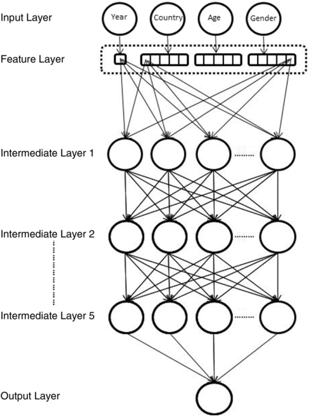
In this section, we describe the fitting of the neural networks in more detail. In total, six networks were fit to the HMD data. Two networks following equations (4)–(6) consist of two intermediate layers, the first of these network models using ReLU activations (DEEP1, in what follows), and the second one using tanh activations (DEEP2). The next two neural network models add three more intermediate layers to each of these first two networks, bringing the number of intermediate layers to five (respectively DEEP3 (ReLU) and DEEP4 (tanh)). We depict these deeper neural networks in Figure 2. Finally, we add a so-called “skip” connection to these deeper networks, by connecting the feature layer directly to the last intermediate layer, as well as to the first intermediate layer (respectively DEEP5 (ReLU) and DEEP6 (tanh)). Skip connections, in various configurations, have been used in the computer vision literature to train very deep neural networks successfully, see for example, He et al. (Reference He, Zhang, Ren and Sun2015), Huang et al. (Reference Huang, Liu and Weinberger2016), and are thought to resolve the vanishing gradient problem that affects deeper networks (Huang et al. Reference Huang, Liu and Weinberger2016) by shortening the path that the back-propagation algorithm needs to follow to get back to the first layer of the network. The code for fitting the DEEP6 network in Keras appears in the appendix in Listing 2.

Figure 2. Five layer deep neural network depicted graphically. The feature layer consists of five dimensional embeddings for each categorical variable, and a single dimension for Year, which is the only numerical variable. Note that for clarity, only some of the connections between the feature and intermediate layers have been shown; also, dropout and batch normalisation layers are not shown.

Listing 2: Deep neural networkmodel with tanh activations and a skip connection (DEEP6).

When fitting the neural networks, the Adam optimiser (Kingma & Ba Reference Kingma and Ba2014) was used, with the parameter values taken at the defaults. The models were each fit for 50 epochs, and the model with the best performance during these 50 epochs, as measured by the validation set, was used. A 5% random sample of the training set was used as a validation set; in other words, the network was fit on 95% of the training set data, comprising 325,090 samples, and performance was assessed on 5% of the training set, comprising 17,110 samples.

Remark 4.1. The neural network is thus fit on slightly less data than the LC, ACF and CAE models and is, therefore, not on entirely equal footing. Although the validation set could be excluded for the models fit using GNMs and back-propagation, it cannot be excluded when fitting the models using SVD (which cannot be applied in the presence of missing values), and, therefore, it was decided to include the validation set for all of the models except the neural network approach.

Since several different network architectures can be fit to the HMD data, it is necessary to choose an optimal architecture against which to test the models mentioned in the previous section; however, as described next, it is not straightforward to choose the optimal model.

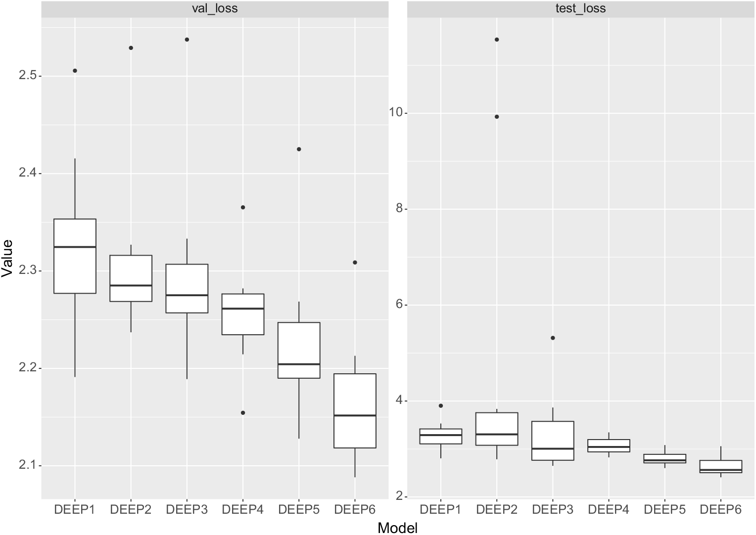
Firstly, we note that the results of training a neural network are somewhat variable (which is due to the initial value of the optimisation algorithm, the random selection of batches of training data to calculate the gradients used in back-propagation, as well as due to dropout, which is applied at random to the neurons of each network), and, therefore, both the in-sample and out-of-sample performance of a neural network can vary somewhat between training attempts. While we note that the reproducibility of the results could be guaranteed by setting the seed value of the random number generator used when fitting the model, there is the possibility that fitting a neural network only once will produce results that are not representative of the model’s average performance (see Figure 3 for an illustration of the potential variability of the results run with 10 different seeds). Thus, in what follows, we fit each network 10 times and take the average MSE to indicate the likely performance of each architecture.

Figure 3. Boxplot of the results of round 1 of training the neural networks described in text for 10 runs on data from 1950 to 1990: left shows validation losses, right shows losses on test data from 1991 to 1999.

Secondly, the training, validation and test sets need to be defined. Since we seek the model that best forecasts the HMD data in the years from 2000 onwards, and we have access to the actual observations in these years, one might propose to use the mortality rates in these years as the test set. However, in a realistic forecasting scenario, the data which are being forecast have not yet been observed, and this approach will not work. Therefore, the training set must be used to determine an optimal model. We approach this by fitting the networks in two rounds, as described next.

In round 1, we split the training set (consisting of data from 1950 to 1999) into a second training set (consisting of data from 1950 to 1990) and test set (consisting of data from 1991 to 1999). We note that in this second training set, three countries have less than 10 years of data (Greece with 9 years of data and Israel and Slovenia each with 7 years of data), but the available data should be sufficient for the purpose of determining the performance of each architecture. As just mentioned, a 5% sample of the training data was taken as a validation set to track when the network has fit the training data appropriately, that is, to indicate over-fitting to the training data. All six networks were fit on the training data, and then the forecasting performance was assessed on the test set from 1991 to 1999. These results are shown in Table 4 and Figure 3, where it can be seen that both DEEP5 and DEEP6 perform well. The optimal forecasting (i.e. out-of-sample and out-of-time) performance, as measured by the test set loss, is achieved by DEEP5, which is the five layer network with ReLU activations and a skip connection, which somewhat improves on the performance of DEEP3, which is a ReLU network without skip connection. However, the best validation performance, by a substantial margin, is the DEEP6 network which is the five layer network with tanh activations and a skip connection, the performance of which is improved dramatically by the skip connection. As already mentioned, we finally note that the results shown in Table 4 represent the average of 10 runs of a random training process, and it is possible that training only a single network will produce less optimal performance, as can be seen by the outliers in Figure 3.

Table 4. Round 1 of fitting the deep neural networks (1950–1990): validation and test set MSEs of the six deep neural network architectures described in the text is shown, averaged over ten training runs; MSE values aremultiplied by 10⁴

In a realistic forecasting scenario, we would now refit only the best neural network architecture (DEEP5) to all of the training data up to year 2000 (unless we wished to use an ensemble of models, in which case we would use the results of more than one model); however, we wish to confirm in this work that the proposed model selection strategy is valid. Therefore, in round 2, we fit all six networks on the full training set (i.e. on the data from 1950 to 1999) and assess the forecasting performance on the test set (years 2000 onwards). These results are shown in Table 5 and Figure 4. The best model in round 2, as measured by the MSE is DEEP6, followed closely by DEEP5. Thus, the results show that the round 1 testing was roughly indicative of the optimal model architecture, leading us to select the second best model, but, unfortunately, not leading us to select DEEP6, which has slightly more optimal performance.

Table 5. Round 2 of fitting the deep neural networks (1950–1999): validation and test set MSEs of the six deep neural network architectures described in the text are shown; MSE values aremultiplied by 10⁴

Figure 4. Boxplot of the results of round 2 of training the neural networks described in text for 10 runs on data from 1950 to 1999: left shows validation losses, right shows losses on test data from 2000 to 2016.

Table 6 shows the results of comparing the DEEP5 neural network results to the rest of the models fit in this section. Note that, for this comparison, we did not average the results of many training runs, but simply selected the results of the first training run. By a wide margin, the best performing model is the deep neural network, which is the optimal model based on the three metrics considered in this section, and produces the best out-of-time forecasts 51 of 76 times (DEEP6 would increase this to 54 of 76 times). In other words, we conclude that for the purposes of large scale mortality forecasting, deep neural network architectures dramatically outperform traditional single and multi-population forecasting models.

Table 6. Comparison of the deep neural network approach with the best models discussed in this section; MSE values aremultiplied by 10⁴

We refer the reader to Appendix B where, as noted above, the deep neural network is compared against the ACF and CAE models, which were modified to use a random walk without a drift term to forecast the country-specific effects. There we conclude similarly that the deep neural network dramatically outperforms the other models, and, indeed, the choice of random walk for forecasting country-specific effects makes little difference to the main conclusion of this section.

5. Discussion and Improving the Neural Network Approach

The previous section has shown that the deep neural network extension of the LC model by far outperforms all of the other models considered in this paper, for the purpose of producing 15-year ahead forecasts. Figure 5 shows the average residuals produced by each of these models, for the ages 0–99 in the period 2000–2016. It can be observed that amongst the models, the deep neural network achieves the smallest residuals, with the fit for females appearing to be better than the fit for males, which is an observation that applies equally to the country and regional LC models. The most significant residuals produced by the neural network are for male teenage and middle-age mortality, where the model predicts rates that are too high, and an emerging trend of predicting rates that are too low at the older ages, in the most recent years, which is in line with recent observations across many countries, see for example, Office for National Statistics (2018). The LC models appear to predict rates that are too low at all ages older than the teenage years, while the ACF and CAE models display a different pattern of residuals that suggest that the model specification has failed to capture the evolution of mortality rates appropriately.

Figure 5. Residuals produced by each of the models, for each gender, year and age separately, averaged over the countries in the HMD.

A cohort effect can be observed in the residuals for all of the models, besides for the neural network, suggesting that part of what the neural network has learned is interactions between Year and Age, which allow the network to model the cohort effect. This observation is confirmed in Figure 6, which displays the average residual for each cohort. The residuals for the neural network are smaller than those produced by the other models and display less of a pattern, suggesting that part of the reason for the out-performance of the neural network is that cohort effects are captured automatically. Nonetheless, some patterns can be observed in these residuals, suggesting that including a cohort effect explicitly may improve the model even further; we refer the reader to the closing remarks of Section 3 for a discussion of how this might be achieved.

Figure 6. Residuals produced by each of the models, for each gender and cohort separately, averaged over the countries in the HMD.

To examine the performance of the neural network in more detail, in Figure 7 the learned parameters of the age embedding are shown, after reducing the dimensionality of the embedding from five dimensions to two dimensions, using PCA. These values do not have an absolute interpretation, since the intermediate layers of the network shift and scale the embedding value (indeed, the values shown are multiplied by −1 to produce the familiar orientation of a life table); however, the values of the embeddings relative to each other are interpretable. The more significant component of the embedding has the familiar shape of a life table and is comparable to the a _x component of the LC model, indicating that the network has learned the overall relationship of mortality rates to each other from the data. The second component appears mainly to capture the relationship between middle age and old age mortality, with mortality rates increasing more quickly with age, as middle age mortality falls, as well as several other relationships between infant, teenage and old age mortality. The learned parameters of the embeddings for age and gender are less interpretable, probably because these parameters only have a meaning in the context of the deeper layers of the neural network.

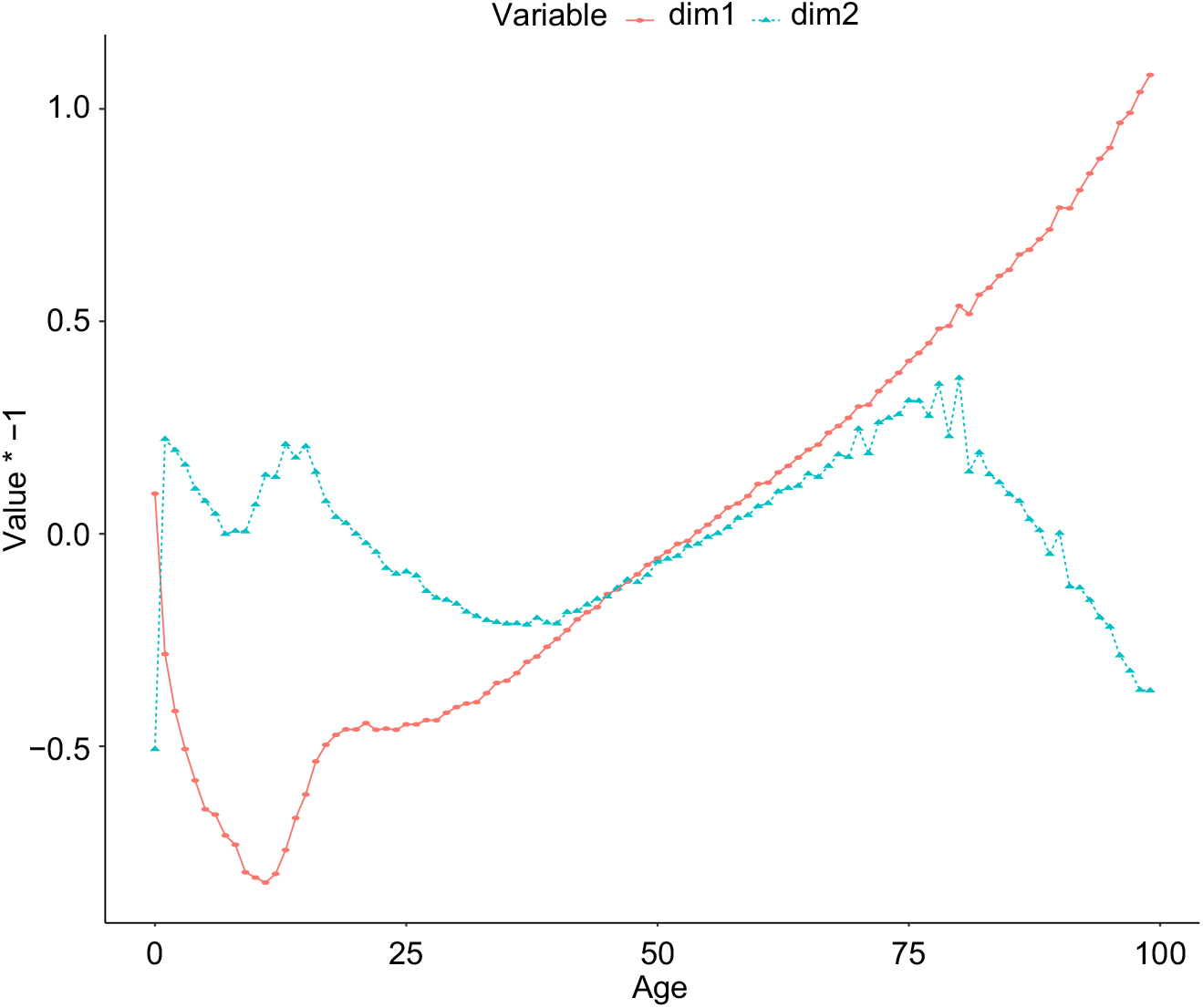
Figure 7. Parameters of the age embedding in the deep neural network, with the dimensionality reduced from 5 to 2 using Principal Components Analysis.

6. Conclusion and Outlook

This paper has shown how the LC model can be extended to work reliably with multiple populations using deep neural networks. Rather than attempting to specify exactly how the inputs to the model determine mortality, as in the case of the original LC model and its extensions to multiple populations, the deep neural network successfully learns these relationships and projects mortality for all countries in the HMD with a high degree of accuracy.

Since many neural network architectures may be chosen, in this study we use a model selection procedure to choose an optimal architecture that eventually proves to be close to the optimal model, amongst those tested. Future research should examine the model selection process in more detail, and it may be the case that a less heuristic selection procedure can be proposed. We also note that an extensive search over neural architectures has not been performed in this study, and only several models were tested. A more comprehensive search over architectures, including models with more layers, difference configurations of skip connections (perhaps following more closely the architectures in He et al. (Reference He, Zhang, Ren and Sun2015) and Huang et al. (Reference Huang, Liu and Weinberger2016)) and different hyper-parameter settings for dropout and learning rates, may produce results that are more optimal than those presented here.

Another avenue for improving forecasting ability is the ensembling together of several neural networks. Although we do not report these results in detail, forecasting rates as the average of the predictions of the DEEP5 and DEEP6 networks produces the best forecasts in 56 of 76 countries, which is better than the results of the DEEP5 and DEEP6 models stand alone. A similar approach would average the results over several of the same networks, which would help to reduce some of the variability in the models that we note in section 4.2 (see, for example, Guo & Berkhahn (Reference Guo and Berkhahn2015) who average the results of 5 of the same neural network architecture in an application of deep networks to structured data).

Other improvements to the model are the inclusion of an explicit cohort effect, as noted in Section 5 and including regional effects within the neural model, which were shown in Section 4.1 to be an important feature within mortality forecasting models. Another useful extension is to model mortality rates in smaller geographic areas, such as states and provinces.

Although we have focused on the LC model in this study, the LC model is not fundamental to the approach that has been proposed, and in future research, one should extend this to other mortality models using neural networks. Finally, an important issue for actuaries and demographers which we have not addressed is the uncertainty of the predictions of the neural network model, and future research should consider how this may be derived.