


1. Introduction
Rotor wakes are dominated by tip vortices, which can play an important role in the performance of a helicopter. A slice through these blade-tip vortices reveals three distinct regions (Ramasamy, Timothy & Leishman Reference Ramasamy, Timothy and Leishman2007; Ramasamy, Johnson & Leishman Reference Ramasamy, Johnson and Leishman2009b ): a laminar inner region (Ragab & Sreedhar Reference Ragab and Sreedhar1995; Devenport et al. Reference Devenport, Rife, Liapis and Follin1996), a second intermediate region that is intermittently transitional (comprising coherent eddies of various scales), and an outer region that is turbulent (less coherent eddies). Devenport et al. (Reference Devenport, Rife, Liapis and Follin1996) suggests that the fluctuations (within the vortex core) are a result of inactive motions produced by the turbulence in the outer wake (surrounding the core), while Bandyopadhyay, Stead & Robert (Reference Bandyopadhyay, Stead and Robert1991) point out that the vortex core comprises intermittent patches of turbulent and relaminarized fluid due to the intermittent exchange of momentum (by organized motions) between the outer turbulent region and the vortex core. Aside from their localized characteristics, these vortices form compact filaments that wander under the influence of both short- and long-wave instabilities (Widnall Reference Widnall1972), all the while interacting with Taylor–Görtler vortices that reside in the trailed vortex sheet behind the rotor blade (Hall Reference Hall1982; Ramasamy et al. Reference Ramasamy, Johnson and Leishman2009b ).
If the vortex core is laminar, then the occurrence of high-velocity fluctuations inside the core is likely to be caused by the formation of short-wave instabilities. Short-wave instabilities form when a vortex filament is subject to a stationary external strain field (Moore & Saffman Reference Moore and Saffman1975; Tsai & Widnall Reference Tsai and Widnall1976). In the case of a helical vortex filament, such as in rotor wakes, strain is inherently induced by three mechanisms: (i) the proximity of the vortex to neighbouring vortices (or its own in the case of a single-bladed rotor), (ii) curvature of the vortex filament, and (iii) torsion (Fukumoto & Okulov Reference Fukumoto and Okulov2005). This causes streamlines to deform elliptically on a plane perpendicular to the vortex axis, and so the vortex filament becomes the subject of the so-called elliptic instability (Bayly Reference Bayly1986; Pierrehumbert Reference Pierrehumbert1986; Leweke & Williamson Reference Leweke and Williamson1998; Kerswell Reference Kerswell2002). Elliptic instabilities have been studied analytically, numerically and experimentally in a variety of bounded and unbounded strained vortex flows (Kerswell Reference Kerswell2002; Lacaze, Ryan & Dizes Reference Lacaze, Ryan and Dizes2007; Roy et al. Reference Roy, Leweke, Thompson and Hourigan2011). In the context of rotor-tip vortices, there are limited quantitative experimental studies characterizing the behaviour of these instabilities and over extended vortex ages.
The objective of the current study is to better understand both the organized turbulence as well as the short-wave instabilities that reside within the vortex produced by a rotor blade in hover. The vortex studied here is formed by a single-bladed rotor and is captured by way of particle image velocimetry (PIV). The advantage of such a configuration is that it reduces the interference from instabilities formed by the presence of other vortex filaments, as is the case with multi-bladed rotors (Martin et al. Reference Martin, Leishman, Pugliese and Anderson2000; Ramasamy et al. Reference Ramasamy, Johnson and Leishman2009b ). Proper orthogonal decomposition (POD) is utilized to flush out the more energetic flow features responsible for characterizing the bulk motions of the tip vortex and is performed over extended vortex ages. The current study is complementary to the one conducted by Roy et al. (Reference Roy, Leweke, Thompson and Hourigan2011), who used dye images to determine the low-order features associated with tip vortices from a fixed wing.
2. Experimental arrangement
The data analysed here were acquired experimentally in a room measuring
 $6.5\times 8.0\times 6.5$
rotor diameters; a schematic of this is shown in figure 1. The set-up comprised a 1.0 m diameter (
$6.5\times 8.0\times 6.5$
rotor diameters; a schematic of this is shown in figure 1. The set-up comprised a 1.0 m diameter (
 $D=2R$
) single-bladed rotor (untwisted NACA 0012 airfoil with a constant chord of
$D=2R$
) single-bladed rotor (untwisted NACA 0012 airfoil with a constant chord of
 $c=52~\text{mm}$
and square tip) attached at the hub by a flap hinge. The rotor was balanced with a counterweight (statically up to 99 %) and was operated at
$c=52~\text{mm}$
and square tip) attached at the hub by a flap hinge. The rotor was balanced with a counterweight (statically up to 99 %) and was operated at
 ${\it\Omega}=1500$
revolutions per minute. This corresponds to a tip chord Reynolds number (
${\it\Omega}=1500$
revolutions per minute. This corresponds to a tip chord Reynolds number (
 $\mathit{Re}_{c}$
) of 218 000 and a tip Mach number of 0.23. The blade was set to a collective pitch angle of
$\mathit{Re}_{c}$
) of 218 000 and a tip Mach number of 0.23. The blade was set to a collective pitch angle of
 $7.3^{\circ }$
, thus resulting in a blade loading (
$7.3^{\circ }$
, thus resulting in a blade loading (
 $C_{T}/{\it\sigma}$
) of 0.066, as measured by a fixed-frame load cell.
$C_{T}/{\it\sigma}$
) of 0.066, as measured by a fixed-frame load cell.

Figure 1. Schematic of the experimental set-up and coordinate transformation.
Velocity measurements were performed along a two-dimensional slice of the rotor wake (along a plane normal to the vortex filament axis) by phase-aligning the rotor with a PIV system using a
 $1/\text{rev}$
optical switch. The orientation of the PIV system (laser and camera) relative to the measurement window is shown in figure 1. The laser sheet was oriented such that it was aligned along the quarter-chord of the blade at 0° vortex age. The focal distance of the PIV camera was chosen to capture only one vortex (including provisions for vortex wander) so as not to compromise on spatial resolution. At each vortex age, the camera was repositioned by way of a two-degree-of-freedom traverse so that the new vortex location was centred on the camera image. Measurement accuracies are estimated to be within
$1/\text{rev}$
optical switch. The orientation of the PIV system (laser and camera) relative to the measurement window is shown in figure 1. The laser sheet was oriented such that it was aligned along the quarter-chord of the blade at 0° vortex age. The focal distance of the PIV camera was chosen to capture only one vortex (including provisions for vortex wander) so as not to compromise on spatial resolution. At each vortex age, the camera was repositioned by way of a two-degree-of-freedom traverse so that the new vortex location was centred on the camera image. Measurement accuracies are estimated to be within
 $0.3^{\circ }$
in azimuth given the inter-frame timing (
$0.3^{\circ }$
in azimuth given the inter-frame timing (
 $36~{\rm\mu}\text{s}$
) between successive laser pulses (laser sheet thickness of 2 mm) and the rotation speed of the rotor. For the current set-up, misalignment of the measurement plane (in
$36~{\rm\mu}\text{s}$
) between successive laser pulses (laser sheet thickness of 2 mm) and the rotation speed of the rotor. For the current set-up, misalignment of the measurement plane (in
 $z^{\prime }$
direction) relative to the calibration plane is of the order of the laser sheet thickness. Based on the object distance (
$z^{\prime }$
direction) relative to the calibration plane is of the order of the laser sheet thickness. Based on the object distance (
 $z_{o}=905~\text{mm}$
) and following § 2.2 in Discetti & Adrian (Reference Discetti and Adrian2012), the resultant magnification error was found to be less than 0.2 %.
$z_{o}=905~\text{mm}$
) and following § 2.2 in Discetti & Adrian (Reference Discetti and Adrian2012), the resultant magnification error was found to be less than 0.2 %.
Seeding was provided by a PIVTEC 14 cascadable Laskin nozzle olive oil seeder, which produced
 $1~{\rm\mu}\text{m}$
diameter particles. These small particles minimize particle tracking errors that are inherent to vortex-dominated flows (Leishman Reference Leishman1996). A check for peak locking errors was performed to ensure that particle image displacements were unbiased by the integer pixel dimension. Additional details concerning these measurements are described by Mula et al. (Reference Mula, Stephenson, Tinney and Sirohi2013).
$1~{\rm\mu}\text{m}$
diameter particles. These small particles minimize particle tracking errors that are inherent to vortex-dominated flows (Leishman Reference Leishman1996). A check for peak locking errors was performed to ensure that particle image displacements were unbiased by the integer pixel dimension. Additional details concerning these measurements are described by Mula et al. (Reference Mula, Stephenson, Tinney and Sirohi2013).
Because of the relatively low blade loading on the rotor, the helical pitch (
 $\hat{p}=H/(2{\rm\pi}R_{c})=0.046$
, where
$\hat{p}=H/(2{\rm\pi}R_{c})=0.046$
, where
 $H$
is the vertical displacement of the helix over one rotor revolution and
$H$
is the vertical displacement of the helix over one rotor revolution and
 $R_{c}=[1+(H/(2{\rm\pi}R))^{2}]R$
is the radius of curvature) and vortex filament torsion (
$R_{c}=[1+(H/(2{\rm\pi}R))^{2}]R$
is the radius of curvature) and vortex filament torsion (
 $\hat{{\it\tau}}=P/R=0.046$
using
$\hat{{\it\tau}}=P/R=0.046$
using
 $P=H/(2{\rm\pi})$
as the reduced pitch) were also small so that the measurement plane was nearly orthogonal to the vortex axis (Leishman, Baker & Coyne Reference Leishman, Baker and Coyne1996; Han, Leishman & Coyne Reference Han, Leishman and Coyne1997; Mula et al.
Reference Mula, Stephenson, Tinney and Sirohi2013). The resultant angle of inclination between the vortex axis and a line normal to the measurement plane was estimated to be
$P=H/(2{\rm\pi})$
as the reduced pitch) were also small so that the measurement plane was nearly orthogonal to the vortex axis (Leishman, Baker & Coyne Reference Leishman, Baker and Coyne1996; Han, Leishman & Coyne Reference Han, Leishman and Coyne1997; Mula et al.
Reference Mula, Stephenson, Tinney and Sirohi2013). The resultant angle of inclination between the vortex axis and a line normal to the measurement plane was estimated to be
 $2.66^{\circ }$
. A total of 350 statistically independent PIV snapshots were acquired at each of the 10 vortex ages studied,
$2.66^{\circ }$
. A total of 350 statistically independent PIV snapshots were acquired at each of the 10 vortex ages studied,
 ${\it\psi}=\{45^{\circ },90^{\circ },135^{\circ },180^{\circ },225^{\circ },270^{\circ },315^{\circ },405^{\circ },495^{\circ },585^{\circ }\}$
, using a field of view of
${\it\psi}=\{45^{\circ },90^{\circ },135^{\circ },180^{\circ },225^{\circ },270^{\circ },315^{\circ },405^{\circ },495^{\circ },585^{\circ }\}$
, using a field of view of
 $88~\text{mm}\times 66~\text{mm}$
. Images were processed using DaVIS v.7.2 with an initial window size of
$88~\text{mm}\times 66~\text{mm}$
. Images were processed using DaVIS v.7.2 with an initial window size of
 $64~\text{pixel}\times 64~\text{pixel}$
that iteratively reduced to a final window size of
$64~\text{pixel}\times 64~\text{pixel}$
that iteratively reduced to a final window size of
 $16~\text{pixel}\times 16~\text{pixel}$
with 50 % overlap. The resulting measurement resolution (
$16~\text{pixel}\times 16~\text{pixel}$
with 50 % overlap. The resulting measurement resolution (
 $L_{m}$
) was found to be 0.88 mm (
$L_{m}$
) was found to be 0.88 mm (
 $\text{grid resolution}=L_{m}/2$
). Spurious vectors were filtered by first establishing a threshold signal-to-noise ratio (set to 1.5), followed by the removal of groups (of less than five vectors) that then ended with a four-pass regional median filter (Westerweel Reference Westerweel1994; Nogueira, Lecuona & Rodriguez Reference Nogueira, Lecuona and Rodriguez1997). This often occurred in the inner core of the vortex due to the poor seeding levels that arise from centrifugal forces (see figure 2 in Mula et al.
Reference Mula, Stephenson, Tinney and Sirohi2013). Missing vectors were then interpolated using a nearest-neighbour fit. Figure 2(a,b) demonstrates a sample raw PIV vector map (subsampled and filtering enabled), and the resultant vector map (after interpolation and smoothing) that was used for subsequent analysis. The post-processed vector map is shown to fit the overall flow structure quite well.
$\text{grid resolution}=L_{m}/2$
). Spurious vectors were filtered by first establishing a threshold signal-to-noise ratio (set to 1.5), followed by the removal of groups (of less than five vectors) that then ended with a four-pass regional median filter (Westerweel Reference Westerweel1994; Nogueira, Lecuona & Rodriguez Reference Nogueira, Lecuona and Rodriguez1997). This often occurred in the inner core of the vortex due to the poor seeding levels that arise from centrifugal forces (see figure 2 in Mula et al.
Reference Mula, Stephenson, Tinney and Sirohi2013). Missing vectors were then interpolated using a nearest-neighbour fit. Figure 2(a,b) demonstrates a sample raw PIV vector map (subsampled and filtering enabled), and the resultant vector map (after interpolation and smoothing) that was used for subsequent analysis. The post-processed vector map is shown to fit the overall flow structure quite well.

Figure 2. (a) Sample original vector map (subsampled) at
 ${\it\psi}=45^{\circ }$
with (b) corresponding post-processed vector map. The vortex centre and core boundary are also identified. (c) Standard deviation of vortex wander along the principal major (♢, ——) and minor (▵,
${\it\psi}=45^{\circ }$
with (b) corresponding post-processed vector map. The vortex centre and core boundary are also identified. (c) Standard deviation of vortex wander along the principal major (♢, ——) and minor (▵,
 $\cdots \cdots$
) axes.
$\cdots \cdots$
) axes.
3. Vortex characteristics
Vortex wander is an inactive motion of the vortex that produces artificially high-velocity fluctuations in the vortex core (Devenport et al.
Reference Devenport, Rife, Liapis and Follin1996). Corrections for this were implemented here using an integral-based approach (the
 ${\it\Gamma}_{1}$
method) that allowed for the vortex centres to be identified; the details of this are described elsewhere (Graftieaux, Michard & Grosjean Reference Graftieaux, Michard and Grosjean2001; Mula et al.
Reference Mula, Stephenson, Tinney and Sirohi2013). Previous studies using multi-bladed rotors have shown the vortex wandering motion to be anisotropic (Kindler, Mulleners & Richard Reference Kindler, Mulleners and Richard2010; Mula et al.
Reference Mula, Stephenson, Tinney and Sirohi2013). Similar results are observed here, where figure 2(c) shows the standard deviation of wander along the principal major and minor axes across all vortex ages. A third-order least-squares fit has also been added (identified by the solid and dashed lines) to help with the interpretation. This wandering motion is shown to grow linearly along the principal minor axis. Wander along the major axis grows faster than that of the minor axis at earlier vortex ages. However, the wandering motion (along the major axis) does not appear to show a continuous growth, as it deviates from the least-squares fit in the vicinity of the first blade passage (360°). It is postulated that this discontinuity is the consequence of long-wave instabilities with non-integer wavenumbers (Bhagwat & Leishman Reference Bhagwat and Leishman2000). The growth rate of these long-wave instabilities has been shown to manifest a local minimum near the first blade passage, which is evident in figure 2(c).
${\it\Gamma}_{1}$
method) that allowed for the vortex centres to be identified; the details of this are described elsewhere (Graftieaux, Michard & Grosjean Reference Graftieaux, Michard and Grosjean2001; Mula et al.
Reference Mula, Stephenson, Tinney and Sirohi2013). Previous studies using multi-bladed rotors have shown the vortex wandering motion to be anisotropic (Kindler, Mulleners & Richard Reference Kindler, Mulleners and Richard2010; Mula et al.
Reference Mula, Stephenson, Tinney and Sirohi2013). Similar results are observed here, where figure 2(c) shows the standard deviation of wander along the principal major and minor axes across all vortex ages. A third-order least-squares fit has also been added (identified by the solid and dashed lines) to help with the interpretation. This wandering motion is shown to grow linearly along the principal minor axis. Wander along the major axis grows faster than that of the minor axis at earlier vortex ages. However, the wandering motion (along the major axis) does not appear to show a continuous growth, as it deviates from the least-squares fit in the vicinity of the first blade passage (360°). It is postulated that this discontinuity is the consequence of long-wave instabilities with non-integer wavenumbers (Bhagwat & Leishman Reference Bhagwat and Leishman2000). The growth rate of these long-wave instabilities has been shown to manifest a local minimum near the first blade passage, which is evident in figure 2(c).
The average spatial topography of the mean vorticity and turbulent kinetic energy per unit mass (
 $\text{TKE}=0.5\langle u_{1}^{2}+u_{2}^{2}\rangle$
with
$\text{TKE}=0.5\langle u_{1}^{2}+u_{2}^{2}\rangle$
with
 $u_{i=1,2}$
being the in-plane fluctuating velocity components), for vortices captured at
$u_{i=1,2}$
being the in-plane fluctuating velocity components), for vortices captured at
 ${\it\psi}=180^{\circ }$
and 495°, are shown in figure 3(a–d) after wander correction. A noticeable asymmetry is observed, which persisted across all other vortex ages (not shown). Core boundaries are identified by the locations of peak swirl velocity and so it is evident in figure 3(c,d) that TKE levels peak inside the vortex core (Devenport et al.
Reference Devenport, Rife, Liapis and Follin1996; Han et al.
Reference Han, Leishman and Coyne1997; Ramasamy et al.
Reference Ramasamy, Johnson and Leishman2009b
). These same features are observed in figure 4(a,b), which shows slices across the average swirl velocity and TKE at
${\it\psi}=180^{\circ }$
and 495°, are shown in figure 3(a–d) after wander correction. A noticeable asymmetry is observed, which persisted across all other vortex ages (not shown). Core boundaries are identified by the locations of peak swirl velocity and so it is evident in figure 3(c,d) that TKE levels peak inside the vortex core (Devenport et al.
Reference Devenport, Rife, Liapis and Follin1996; Han et al.
Reference Han, Leishman and Coyne1997; Ramasamy et al.
Reference Ramasamy, Johnson and Leishman2009b
). These same features are observed in figure 4(a,b), which shows slices across the average swirl velocity and TKE at
 ${\it\psi}=180^{\circ }$
and 495°, respectively. It is worth mentioning that the total resolved turbulent kinetic energy, based on the in-plane velocity, varies between 2 % and 8 % of the total resolved kinetic energy associated with the vortex over the range of vortex ages studied.
${\it\psi}=180^{\circ }$
and 495°, respectively. It is worth mentioning that the total resolved turbulent kinetic energy, based on the in-plane velocity, varies between 2 % and 8 % of the total resolved kinetic energy associated with the vortex over the range of vortex ages studied.

Figure 3. (a,b) Mean axial vorticity,
 ${\it\omega}_{z}/{\it\Omega}\times (-0.1)$
at (a)
${\it\omega}_{z}/{\it\Omega}\times (-0.1)$
at (a)
 ${\it\psi}=180^{\circ }$
and (b)
${\it\psi}=180^{\circ }$
and (b)
 ${\it\psi}=495^{\circ }$
. (c,d) Plots of
${\it\psi}=495^{\circ }$
. (c,d) Plots of
 $(\text{TKE}/V_{t}^{2})\times 10^{3}$
at (c)
$(\text{TKE}/V_{t}^{2})\times 10^{3}$
at (c)
 ${\it\psi}=180^{\circ }$
and (d)
${\it\psi}=180^{\circ }$
and (d)
 ${\it\psi}=495^{\circ }$
;
${\it\psi}=495^{\circ }$
;
 $V_{t}$
is the blade-tip velocity.
$V_{t}$
is the blade-tip velocity.

Figure 4. Swirl velocity,
 $(V_{{\it\Theta}}/V_{t})\times 10$
(▿), and
$(V_{{\it\Theta}}/V_{t})\times 10$
(▿), and
 $(\text{TKE}/V_{t}^{2})\times 10^{3}$
(
$(\text{TKE}/V_{t}^{2})\times 10^{3}$
(
 ${\it\xi}$
in figure 3(c,d) at (a)
${\it\xi}$
in figure 3(c,d) at (a)
 ${\it\psi}=180^{\circ }$
and (b)
${\it\psi}=180^{\circ }$
and (b)
 ${\it\psi}=495^{\circ }$
. (c) Comparison of the core radius with the previous studies listed in table 1.
${\it\psi}=495^{\circ }$
. (c) Comparison of the core radius with the previous studies listed in table 1.
As for the core radius, close inspection of figure 4(c) shows a monotonic increase from 10 % to 15 % of the blade chord up until the first rotor revolution (this is after wander correction). A comparison of our findings with those reported in the open literature is also provided; see table 1 for a listing of the rotor operating conditions associated with these studies. At the earliest vortex age studied here (
 ${\it\Psi}=45^{\circ }$
),
${\it\Psi}=45^{\circ }$
),
 $L_{m}/r_{c}=0.17$
(
$L_{m}/r_{c}=0.17$
(
 ${<}0.2$
), which satisfies the measurement resolution requirements suggested by Martin et al. (Reference Martin, Leishman, Pugliese and Anderson2000) for determining core radius. In general, the trends in figure 4(c) are consistent with the open literature. That is, up until the first blade passage (360°), diffusion causes the core radius to increase with increasing vortex age. Aside from the studies of Thompson, Komerath & Gray (Reference Thompson, Komerath and Gray1988) and Richard et al. (Reference Richard, Van der Wall, Raffel and Thimm2008), the core radius is shown to decrease after the first blade passage due to vortex stretching induced by the oncoming blade. The corresponding vortex Reynolds number of our study was found to range between
${<}0.2$
), which satisfies the measurement resolution requirements suggested by Martin et al. (Reference Martin, Leishman, Pugliese and Anderson2000) for determining core radius. In general, the trends in figure 4(c) are consistent with the open literature. That is, up until the first blade passage (360°), diffusion causes the core radius to increase with increasing vortex age. Aside from the studies of Thompson, Komerath & Gray (Reference Thompson, Komerath and Gray1988) and Richard et al. (Reference Richard, Van der Wall, Raffel and Thimm2008), the core radius is shown to decrease after the first blade passage due to vortex stretching induced by the oncoming blade. The corresponding vortex Reynolds number of our study was found to range between
 $8.3\times 10^{4}$
and
$8.3\times 10^{4}$
and
 $8.7\times 10^{4}$
over the vortex ages studied.
$8.7\times 10^{4}$
over the vortex ages studied.
Table 1. Overview of experimental conditions reported by others.

Table 2. Estimates of the binormal induced velocity measured from the current experiment compared with the theoretical predictions using (3.2).

Since the torsion of the helix is very small (
 $\hat{{\it\tau}}=0.046$
), its influence is significant on the binormal induced velocity (of the vortex), which is primarily responsible for the displacement of the vortex filament in a fluid (Ricca Reference Ricca1994). Here, the binormal velocity is computed as the net in-plane velocity of the vortex,
$\hat{{\it\tau}}=0.046$
), its influence is significant on the binormal induced velocity (of the vortex), which is primarily responsible for the displacement of the vortex filament in a fluid (Ricca Reference Ricca1994). Here, the binormal velocity is computed as the net in-plane velocity of the vortex,
 $$\begin{eqnarray}\boldsymbol{v}_{b}=\frac{1}{A}\iint \boldsymbol{U}(x^{\prime },y^{\prime })\,\text{d}x^{\prime }\,\text{d}y^{\prime },\quad A=\iint \text{d}x^{\prime }\,\text{d}y^{\prime },\end{eqnarray}$$
where
 $\boldsymbol{U}(x^{\prime },y^{\prime })$
is the mean (in-plane) velocity field within the vortex,
$\boldsymbol{U}(x^{\prime },y^{\prime })$
is the mean (in-plane) velocity field within the vortex,
 $A$
is the area of the vortex, and the limits of integration are confined to
$A$
is the area of the vortex, and the limits of integration are confined to
 ${\sim}2r_{c}$
(from the vortex centre). The dimensionless binormal velocity is then estimated using
${\sim}2r_{c}$
(from the vortex centre). The dimensionless binormal velocity is then estimated using
 $\hat{v}_{b}=|\boldsymbol{v}_{b}|4{\rm\pi}R_{c}/{\it\Gamma}_{v}$
and is provided in table 2 at various vortex ages throughout the measurement envelope using
$\hat{v}_{b}=|\boldsymbol{v}_{b}|4{\rm\pi}R_{c}/{\it\Gamma}_{v}$
and is provided in table 2 at various vortex ages throughout the measurement envelope using
 ${\it\Gamma}_{v}$
as the circulation strength of the vortex. A comparison of our estimates with the theoretical predictions is also provided based on the following analytical expression from Ricca (Reference Ricca1994),
${\it\Gamma}_{v}$
as the circulation strength of the vortex. A comparison of our estimates with the theoretical predictions is also provided based on the following analytical expression from Ricca (Reference Ricca1994),
 $$\begin{eqnarray}\hat{v}_{b}=\log \frac{R_{c}}{r_{c}}+C_{MS},\end{eqnarray}$$
where
 $C_{MS}$
depends on the geometry of the helix and is determined using the closed analytical expression
$C_{MS}$
depends on the geometry of the helix and is determined using the closed analytical expression
 $$\begin{eqnarray}C_{MS}=-{\textstyle \frac{1}{4}}+\hat{p}^{-1}+\log \hat{p}+1-{\textstyle \frac{1}{2}}\hat{p}+[{\textstyle \frac{3}{8}}{\it\zeta}(3)-{\textstyle \frac{1}{2}}]\hat{p}^{2}-{\textstyle \frac{5}{8}}\hat{p}^{3}+O(\hat{p}^{4})\end{eqnarray}$$
derived by Boersma & Wood (Reference Boersma and Wood1999) for thin helical filaments of small pitch. These theoretical estimates are shown to compare favourably with our laboratory measurements.
4. POD of a spiralling vortex
Lumley’s (Reference Lumley, Yaglom and Tatarsky1967) POD is used here to identify the most energetic features of the turbulence fluctuations that reside within the blade-tip vortex. The technique has been rigorously used in both the experimental and numerical disciplines, with an extensive description of its mathematical intricacies having been provided by Berkooz, Holmes & Lumley (Reference Berkooz, Holmes and Lumley1993). In the current study, we follow the approach outlined by Glauser & George (Reference Glauser, George, Comte-Bellot and Mathieu1987), Citriniti & George (Reference Citriniti and George2000) and Tinney, Glauser & Ukeiley (Reference Tinney, Glauser and Ukeiley2008), whereby the vortex (and its surrounding fluid) is first decomposed in azimuth using Fourier decomposition followed by a radial decomposition using POD. This is applied to only the fluctuating part of the signal and after correcting for wander; the effect of vortex wandering correction on the results presented here is discussed in the Appendix A. While it is customary for one to use the snapshot POD (Sirovich Reference Sirovich1987) approach with PIV data, (given the tradeoff between spatial resolution and the number of realizations), the spatial modes described by harmonic analysis are more easily interpreted.
The process begins by first transforming the raw PIV images from Cartesian coordinates to cylindrical coordinates (i.e.
 $x^{\prime },y^{\prime },z^{\prime }~\rightarrow ~r,{\it\theta},z^{\prime }$
). At each vortex age, the azimuthal grid resolution,
$x^{\prime },y^{\prime },z^{\prime }~\rightarrow ~r,{\it\theta},z^{\prime }$
). At each vortex age, the azimuthal grid resolution,
 ${\it\delta}{\it\theta}$
, is determined such that it equals the resolution of the original grid at
${\it\delta}{\it\theta}$
, is determined such that it equals the resolution of the original grid at
 $r=r_{c}$
,
$r=r_{c}$
,
 ${\it\delta}{\it\theta}=\tan ^{-1}(L_{m}/(2r_{c}))$
. For example, at
${\it\delta}{\it\theta}=\tan ^{-1}(L_{m}/(2r_{c}))$
. For example, at
 ${\it\psi}=135^{\circ }$
,
${\it\psi}=135^{\circ }$
,
 ${\it\delta}{\it\theta}$
is equal to 4° (though it was found to vary only from 3° to 5° over the entire measurement envelope). The fluctuating part of the in-plane velocity field (
${\it\delta}{\it\theta}$
is equal to 4° (though it was found to vary only from 3° to 5° over the entire measurement envelope). The fluctuating part of the in-plane velocity field (
 $u_{i=1,2}$
, where
$u_{i=1,2}$
, where
 $\tilde{u} _{i}=U_{i}+u_{i}$
, and
$\tilde{u} _{i}=U_{i}+u_{i}$
, and
 $1=r$
and
$1=r$
and
 $2={\it\theta}$
) is then transformed along the azimuthal coordinate to obtain the Fourier-azimuthal modes for each of the 350 PIV snapshots at a given vortex age as follows:
$2={\it\theta}$
) is then transformed along the azimuthal coordinate to obtain the Fourier-azimuthal modes for each of the 350 PIV snapshots at a given vortex age as follows:
 $$\begin{eqnarray}\hat{u_{i}}(r,{\it\psi},t;m)=\frac{1}{2{\rm\pi}}\int _{-{\rm\pi}}^{{\rm\pi}}u_{i}(r,{\it\theta},{\it\psi},t)\text{e}^{-\text{i}m{\it\theta}}\,\text{d}{\it\theta},\end{eqnarray}$$
from which a two-point tensor is then formed,
 $$\begin{eqnarray}\unicode[STIX]{x1D609}_{ij}(r,r^{\prime },{\it\psi};m)=\langle \hat{u_{i}}(r,{\it\psi},t;m)\,\hat{u_{j}}^{\ast }(r^{\prime },{\it\psi},t;m)\rangle .\end{eqnarray}$$
Here
 $\langle ~\rangle$
is used to denote ensemble averaging. In (4.1), the same azimuthal starting position is employed in order to preserve the asymmetries that are shown to reside in the TKE profiles in figures 3 and 4. Symmetry considerations for statistically axisymmetric flows without swirl are provided in appendix A of Jung, Gamard & George (Reference Jung, Gamard and George2004). Here we assume these symmetries cannot be applied. An integral eigenvalue problem is then formed for each vortex age,
$\langle ~\rangle$
is used to denote ensemble averaging. In (4.1), the same azimuthal starting position is employed in order to preserve the asymmetries that are shown to reside in the TKE profiles in figures 3 and 4. Symmetry considerations for statistically axisymmetric flows without swirl are provided in appendix A of Jung, Gamard & George (Reference Jung, Gamard and George2004). Here we assume these symmetries cannot be applied. An integral eigenvalue problem is then formed for each vortex age,
 $$\begin{eqnarray}\int _{R}^{}\unicode[STIX]{x1D609}_{ij}(r,r^{\prime },{\it\psi};m)\,{\it\Phi}_{j}^{(n)}(r^{\prime },{\it\psi};m)r^{\prime }\,\text{d}r^{\prime }={\it\Lambda}^{n}({\it\psi};m)\,{\it\Phi}_{i}^{(n)}(r,{\it\psi};m),\end{eqnarray}$$
and is solved to produce an ordered sequence of eigenvalues (
 ${\it\lambda}^{n}\geqslant {\it\lambda}^{n+1}$
) with eigenfunctions
${\it\lambda}^{n}\geqslant {\it\lambda}^{n+1}$
) with eigenfunctions
 ${\it\Phi}_{i}^{n}(r,{\it\psi};m)$
. This vector decomposition ensures that the eigenfunctions, corresponding to the in-plane velocity components, are coupled. In order to construct the spatial modes that characterize the velocity field, the POD eigenfunctions
${\it\Phi}_{i}^{n}(r,{\it\psi};m)$
. This vector decomposition ensures that the eigenfunctions, corresponding to the in-plane velocity components, are coupled. In order to construct the spatial modes that characterize the velocity field, the POD eigenfunctions
 ${\it\Phi}_{i}^{n}$
and Fourier eigenfunctions
${\it\Phi}_{i}^{n}$
and Fourier eigenfunctions
 $\text{e}^{\text{i}m{\it\theta}}$
are combined as follows:
$\text{e}^{\text{i}m{\it\theta}}$
are combined as follows:
 $$\begin{eqnarray}\mathfrak{U}_{i}^{(m,n)}(r,{\it\theta},{\it\psi})=\text{e}^{\text{i}m{\it\theta}}{\it\Phi}_{i}^{(n)}(r,{\it\psi};m).\end{eqnarray}$$
When compared with the spatial modes obtained using the snapshot POD method (which also does not force axisymmetry), the general features of the first few most energetic modes were essentially the same (Mula & Tinney Reference Mula and Tinney2014).
Having discretized (4.3), the total number of POD modes is governed by the product between the number of points measured (
 $N$
) and the number of in-plane components
$N$
) and the number of in-plane components
 $({\it\eta})$
used to construct
$({\it\eta})$
used to construct
 $\unicode[STIX]{x1D609}_{ij}$
. The radial extent is confined to
$\unicode[STIX]{x1D609}_{ij}$
. The radial extent is confined to
 ${\sim}2r_{c}$
at each
${\sim}2r_{c}$
at each
 ${\it\psi}$
. So, given the grid resolution employed here (
${\it\psi}$
. So, given the grid resolution employed here (
 $L_{m}/2$
;
$L_{m}/2$
;
 $L_{m}/r_{c}<0.2$
),
$L_{m}/r_{c}<0.2$
),
 $N>20$
, at least 40 POD modes are generated at each vortex age. Further, the total resolved energy (Citriniti & George Reference Citriniti and George2000; Tinney et al.
Reference Tinney, Glauser and Ukeiley2008) of the flow,
$N>20$
, at least 40 POD modes are generated at each vortex age. Further, the total resolved energy (Citriniti & George Reference Citriniti and George2000; Tinney et al.
Reference Tinney, Glauser and Ukeiley2008) of the flow,
 ${\it\Pi}({\it\psi})$
, and the normalized eigenspectra,
${\it\Pi}({\it\psi})$
, and the normalized eigenspectra,
 ${\it\beta}^{n}({\it\psi};m)$
, are obtained as
${\it\beta}^{n}({\it\psi};m)$
, are obtained as
 $$\begin{eqnarray}{\it\Pi}({\it\psi})=\mathop{\sum }_{n}^{}\mathop{\sum }_{m}^{}{\it\Lambda}^{n}({\it\psi};m),\quad {\it\beta}^{n}({\it\psi};m)=\frac{{\it\Lambda}^{n}({\it\psi};m)}{{\it\Pi}({\it\psi})}.\end{eqnarray}$$
While (4.4) allows one to view the spatial topography of the modes associated with the average turbulence statistics, an instantaneous low-dimensional representation of the fluctuating velocity field can be obtained from the following established expressions (Lumley Reference Lumley, Yaglom and Tatarsky1967),
 $$\begin{eqnarray}\hat{\mathfrak{u}}_{i}(r,{\it\psi},t;m)=\mathop{\sum }_{n=1}^{k}\boldsymbol{a}^{(n)}({\it\psi},t;m)\,{\it\Phi}_{i}^{(n)}(r,{\it\psi};m),\end{eqnarray}$$
using uncorrelated and time-varying coefficients,
 $$\begin{eqnarray}\boldsymbol{a}^{(n)}({\it\psi},t;m)=\int _{R}\hat{u} _{i}(r,{\it\psi},t;m)\,{\it\Phi}_{i}^{(n)\ast }(r,{\it\psi};m)r\,\text{d}r.\end{eqnarray}$$
The mean-square energies of these coefficients are the eigenvalues themselves,
 ${\it\lambda}^{(n)}=\langle \boldsymbol{a}^{(n)}\boldsymbol{a}^{(n)}\rangle$
, while for
${\it\lambda}^{(n)}=\langle \boldsymbol{a}^{(n)}\boldsymbol{a}^{(n)}\rangle$
, while for
 $k={\it\eta}N$
,
$k={\it\eta}N$
,
 $\hat{\mathfrak{u}}_{i}=\hat{u} _{i}$
. A low-dimensional reconstruction of the fluctuating velocity is then obtained using the following inverse transformation:
$\hat{\mathfrak{u}}_{i}=\hat{u} _{i}$
. A low-dimensional reconstruction of the fluctuating velocity is then obtained using the following inverse transformation:
 $$\begin{eqnarray}\mathfrak{u}_{i}(r,{\it\theta},{\it\psi},t)=\mathop{\sum }_{m}\hat{\mathfrak{u}}_{i}(r,{\it\psi},t;m)\text{e}^{\text{i}m{\it\theta}}.\end{eqnarray}$$
4.1. Low-dimensional axial vorticity
Given the kind of flow being studied here and the arrangement of our measurement system, it is only natural that we seek to construct a low-dimensional representation of the axial vorticity. This is calculated using the standard expression
 $$\begin{eqnarray}{{\it\varpi}_{z}}^{(m,n)}=\frac{1}{r}\frac{\partial (r{\mathfrak{U}_{2}}^{(m,n)})}{\partial r}-\frac{1}{r}\frac{\partial {\mathfrak{U}_{1}}^{(m,n)}}{\partial {\it\theta}},\end{eqnarray}$$
with gradients in
 $r$
being determined using a second-order central difference scheme. Contrarily, gradients in
$r$
being determined using a second-order central difference scheme. Contrarily, gradients in
 ${\it\theta}$
are calculated analytically by the nature of Fourier functions,
${\it\theta}$
are calculated analytically by the nature of Fourier functions,
 $$\begin{eqnarray}\frac{\partial \mathfrak{U}_{1}^{(m,n)}}{\partial {\it\theta}}=\text{i}m\,\text{e}^{\text{i}m{\it\theta}}{\it\Phi}_{1}^{(n)}(r,{\it\psi};m).\end{eqnarray}$$
Likewise, the axial vorticity of the low-dimensional instantaneous fluctuating velocity can be calculated by simply replacing
 ${\mathfrak{U}_{i}}^{(m,n)}$
in (4.9) with
${\mathfrak{U}_{i}}^{(m,n)}$
in (4.9) with
 $\mathfrak{u}_{i}$
from (4.8).
$\mathfrak{u}_{i}$
from (4.8).
5. Results
Convergence of the POD modes is shown in figure 5(a), with approximately 75 % of the resolved energy residing in the first POD mode (
 $n=1$
) for the entire range of
$n=1$
) for the entire range of
 ${\it\psi}$
studied here. Given the spatial resolution used to generate
${\it\psi}$
studied here. Given the spatial resolution used to generate
 $\unicode[STIX]{x1D609}_{ij}$
, this rapid convergence is a reflection of the organized events that characterize the active motions of this vortex filament, as opposed to numerical integration errors (see § 4.1 of Tinney et al.
Reference Tinney, Glauser and Ukeiley2008); similar rates of convergence were found at other vortex ages. Furthermore, for the first POD mode (
$\unicode[STIX]{x1D609}_{ij}$
, this rapid convergence is a reflection of the organized events that characterize the active motions of this vortex filament, as opposed to numerical integration errors (see § 4.1 of Tinney et al.
Reference Tinney, Glauser and Ukeiley2008); similar rates of convergence were found at other vortex ages. Furthermore, for the first POD mode (
 $n=1$
), figure 5(b) demonstrates how the helical mode (
$n=1$
), figure 5(b) demonstrates how the helical mode (
 $m=1$
) dominates the energy spectrum (
$m=1$
) dominates the energy spectrum (
 ${>}40\,\%$
) at all vortex ages, followed by the axisymmetric (
${>}40\,\%$
) at all vortex ages, followed by the axisymmetric (
 $m=0$
) and double helical modes (
$m=0$
) and double helical modes (
 $m=2$
). However, at
$m=2$
). However, at
 ${\it\psi}=45^{\circ }$
, both the axisymmetric and helical modes are equally imperative. In what follows we will resort to a viewing of the first few eigenfunctions for an understanding of their behaviour.
${\it\psi}=45^{\circ }$
, both the axisymmetric and helical modes are equally imperative. In what follows we will resort to a viewing of the first few eigenfunctions for an understanding of their behaviour.

Figure 5. (a) Energy spectra of the first seven POD modes. (b) Fourier mode energy spectra of the first (
 $n=1$
) POD mode for
$n=1$
) POD mode for
 $m=0$
(○), 1 (
$m=0$
(○), 1 (
5.1. Spatial structures of the Fourier modes for the first POD mode
We begin this discussion by presenting the spatial structures of the axisymmetric (
 $m=0$
), helical (
$m=0$
), helical (
 $m=1$
) and double helical (
$m=1$
) and double helical (
 $m=2$
) modes for the first POD mode (
$m=2$
) modes for the first POD mode (
 $n=1$
) using (4.9). Where the axisymmetric mode is concerned, radial profiles of circulation and axial vorticity are shown in figure 6(a) for
$n=1$
) using (4.9). Where the axisymmetric mode is concerned, radial profiles of circulation and axial vorticity are shown in figure 6(a) for
 ${\it\psi}=45^{\circ }$
. These profiles resemble that of a vortex with viscous core (see Han et al.
Reference Han, Leishman and Coyne1997; Ramasamy et al.
Reference Ramasamy, Timothy and Leishman2007). Hence, the axisymmetric mode is associated with the roll-up of the vortex sheet trailed from the rotor blade at early ages. However, at
${\it\psi}=45^{\circ }$
. These profiles resemble that of a vortex with viscous core (see Han et al.
Reference Han, Leishman and Coyne1997; Ramasamy et al.
Reference Ramasamy, Timothy and Leishman2007). Hence, the axisymmetric mode is associated with the roll-up of the vortex sheet trailed from the rotor blade at early ages. However, at
 ${\it\psi}=315^{\circ }$
in figure 6(b) (after the roll-up process is complete), circulation and vorticity profiles associated with the axisymmetric mode manifest the kinds of behaviours observed in swirling jet flows (Liang & Maxworthy Reference Liang and Maxworthy2005). The presence of this swirling jet mode, which is shown in figure 5(b) to increase in energy from 5 % (at
${\it\psi}=315^{\circ }$
in figure 6(b) (after the roll-up process is complete), circulation and vorticity profiles associated with the axisymmetric mode manifest the kinds of behaviours observed in swirling jet flows (Liang & Maxworthy Reference Liang and Maxworthy2005). The presence of this swirling jet mode, which is shown in figure 5(b) to increase in energy from 5 % (at
 ${\it\psi}=90^{\circ }$
) to about 15 % (at
${\it\psi}=90^{\circ }$
) to about 15 % (at
 ${\it\psi}=495^{\circ }$
), reinforces flow entrainment and diffusion mechanisms.
${\it\psi}=495^{\circ }$
), reinforces flow entrainment and diffusion mechanisms.

Figure 6. Radial profiles of axial vorticity (○) and circulation (▫) for
 $(m,n)=(0,1)$
at (a) 45° and (b) 315° age.
$(m,n)=(0,1)$
at (a) 45° and (b) 315° age.
Owing to the nature of Fourier functions, non-zero Fourier modes such as the helical (
 $m=1$
) or double helical modes (
$m=1$
) or double helical modes (
 $m=2$
) comprise both real and imaginary components. Figure 7 shows the real component of the axial vorticity of the helical mode at a sample vortex age (
$m=2$
) comprise both real and imaginary components. Figure 7 shows the real component of the axial vorticity of the helical mode at a sample vortex age (
 ${\it\psi}=135^{\circ }$
). As expected, the spatial structure of the imaginary component is identical to its real counterpart, except that it is oriented at
${\it\psi}=135^{\circ }$
). As expected, the spatial structure of the imaginary component is identical to its real counterpart, except that it is oriented at
 ${\rm\pi}/(2m)=90^{\circ }$
(anticlockwise) relative to its real counterpart. Bayly (Reference Bayly1986), Pierrehumbert (Reference Pierrehumbert1986), Leweke & Williamson (Reference Leweke and Williamson1998), Sipp (Reference Sipp2000) and Kerswell (Reference Kerswell2002) have shown how helical modes, such as the one displayed in figure 7, cause streamlines of the base vortex flow to undergo elliptical deformation. More recently, Lacaze et al. (Reference Lacaze, Ryan and Dizes2007) showed how the most unstable modes associated with the elliptic instability correspond to
${\rm\pi}/(2m)=90^{\circ }$
(anticlockwise) relative to its real counterpart. Bayly (Reference Bayly1986), Pierrehumbert (Reference Pierrehumbert1986), Leweke & Williamson (Reference Leweke and Williamson1998), Sipp (Reference Sipp2000) and Kerswell (Reference Kerswell2002) have shown how helical modes, such as the one displayed in figure 7, cause streamlines of the base vortex flow to undergo elliptical deformation. More recently, Lacaze et al. (Reference Lacaze, Ryan and Dizes2007) showed how the most unstable modes associated with the elliptic instability correspond to
 $|m|=1$
(helical mode) when the axial velocity strength (
$|m|=1$
(helical mode) when the axial velocity strength (
 $W_{0}$
) is low. Here, we estimate
$W_{0}$
) is low. Here, we estimate
 $W_{0}=0.159$
, which is sufficiently low, using the axial velocity data from Mula et al. (Reference Mula, Stephenson, Tinney and Sirohi2013) and see from figure 5(b) that the helical mode dominates the energy spectrum of the vortex filament. So, it is clear that the helical mode in figure 7 is a mode associated with the elliptic instability.
$W_{0}=0.159$
, which is sufficiently low, using the axial velocity data from Mula et al. (Reference Mula, Stephenson, Tinney and Sirohi2013) and see from figure 5(b) that the helical mode dominates the energy spectrum of the vortex filament. So, it is clear that the helical mode in figure 7 is a mode associated with the elliptic instability.

Figure 7. Contours of the (a) real and (b) imaginary components of the axial vorticity of the helical mode
 $(m,n)=(1,1)$
at
$(m,n)=(1,1)$
at
 ${\it\psi}=135^{\circ }$
. Circles of core radius (——) and peak TKE (
${\it\psi}=135^{\circ }$
. Circles of core radius (——) and peak TKE (
 $\cdots \cdots$
) are indicated.
$\cdots \cdots$
) are indicated.
In order to study the evolutionary behaviour of this helical mode, its real component is shown in figure 8 over the range of vortex ages measured. At the earliest vortex age,
 ${\it\psi}=45^{\circ }$
, two counter-rotating eddies are manifest, which reside on the circle of core radius. These eddies remain centred on the core radius for all vortex ages without modifying the structure of the helical mode. Likewise, the size of these eddies increases as the core radius increases. Therefore, the helical mode of the elliptic instability in figure 8 is shown to be in the linear regime; an elliptic instability mode in the nonlinear regime would undergo either a rotation (Sipp Reference Sipp2000) or a modification in its structure (Schaeffer & Dizes Reference Schaeffer and Dizes2010), which is not observed here. Furthermore, where short-wave instabilities are concerned, Hattori & Fukumoto (Reference Hattori and Fukumoto2009, Reference Hattori and Fukumoto2014) have shown how torsion produces a second-order correction to the growth rate of the curvature instability, which is first order in
${\it\psi}=45^{\circ }$
, two counter-rotating eddies are manifest, which reside on the circle of core radius. These eddies remain centred on the core radius for all vortex ages without modifying the structure of the helical mode. Likewise, the size of these eddies increases as the core radius increases. Therefore, the helical mode of the elliptic instability in figure 8 is shown to be in the linear regime; an elliptic instability mode in the nonlinear regime would undergo either a rotation (Sipp Reference Sipp2000) or a modification in its structure (Schaeffer & Dizes Reference Schaeffer and Dizes2010), which is not observed here. Furthermore, where short-wave instabilities are concerned, Hattori & Fukumoto (Reference Hattori and Fukumoto2009, Reference Hattori and Fukumoto2014) have shown how torsion produces a second-order correction to the growth rate of the curvature instability, which is first order in
 ${\it\epsilon}$
(the ratio of core radius to curvature radius). From this, it can be inferred that torsion also influences the growth rate of the elliptic instability, which is of
${\it\epsilon}$
(the ratio of core radius to curvature radius). From this, it can be inferred that torsion also influences the growth rate of the elliptic instability, which is of
 $O({\it\epsilon}^{2}\log (1/{\it\epsilon}))$
(Fukumoto & Hattori Reference Fukumoto and Hattori2005; Hattori & Fukumoto Reference Hattori and Fukumoto2014). Given the amount of torsion in the current set of measurements (
$O({\it\epsilon}^{2}\log (1/{\it\epsilon}))$
(Fukumoto & Hattori Reference Fukumoto and Hattori2005; Hattori & Fukumoto Reference Hattori and Fukumoto2014). Given the amount of torsion in the current set of measurements (
 $\hat{{\it\tau}}=0.046$
), the most unstable mode of elliptic instability (the helical mode) is shown to be in the linear regime for the entire range of vortex ages studied. It is postulated that, by reducing the amount of torsion (of the helix), nonlinearities will develop in this most unstable mode, and will accelerate the breakdown of the tip vortex structure (Leweke & Williamson Reference Leweke and Williamson1998; Schaeffer & Dizes Reference Schaeffer and Dizes2010).
$\hat{{\it\tau}}=0.046$
), the most unstable mode of elliptic instability (the helical mode) is shown to be in the linear regime for the entire range of vortex ages studied. It is postulated that, by reducing the amount of torsion (of the helix), nonlinearities will develop in this most unstable mode, and will accelerate the breakdown of the tip vortex structure (Leweke & Williamson Reference Leweke and Williamson1998; Schaeffer & Dizes Reference Schaeffer and Dizes2010).

Figure 8. Contours of the real component of the axial vorticity of the helical mode
 $(m,n)=(1,1)$
at
$(m,n)=(1,1)$
at
 ${\it\psi}=45^{\circ }{-}495^{\circ }$
. Circles of core radius (——) and peak TKE (
${\it\psi}=45^{\circ }{-}495^{\circ }$
. Circles of core radius (——) and peak TKE (
 $\cdots \cdots$
) are indicated.
$\cdots \cdots$
) are indicated.
While we have shown the evolutionary characteristics of the dominant mode of the elliptic instability, it would be interesting to see how this mode might reveal itself in an instantaneous sense. Therefore, a low-dimensional reconstruction of the instantaneous vorticity field using
 $(m,n)=(1,1)$
at
$(m,n)=(1,1)$
at
 ${\it\psi}=405^{\circ }$
is shown in figure 9(c) and is performed by combining the average vorticity at that vortex age (figure 9
a, with the core boundary identified by
${\it\psi}=405^{\circ }$
is shown in figure 9(c) and is performed by combining the average vorticity at that vortex age (figure 9
a, with the core boundary identified by
 ${\it\tau}_{1}$
) with an instantaneous snapshot of the low-dimensional fluctuating vorticity field (figure 9
b). The boundaries identifying the locations of peak swirl velocity associated with the mean flow (figure 9
a) are shown in figure 9(c) with (
${\it\tau}_{1}$
) with an instantaneous snapshot of the low-dimensional fluctuating vorticity field (figure 9
b). The boundaries identifying the locations of peak swirl velocity associated with the mean flow (figure 9
a) are shown in figure 9(c) with (
 ${\it\tau}_{2}$
) and without (
${\it\tau}_{2}$
) and without (
 ${\it\tau}_{1}$
) the effects imposed by the addition of a low-dimensional fluctuating vorticity field (figure 9
b). The discrepancies between these boundaries coincide with the compression and expansion of contour lines, which is typical of elliptic instability; the inward radial displacement of the instantaneous boundary (from the mean) causes streamline compression, while the outward displacement causes streamline expansion (Leweke & Williamson Reference Leweke and Williamson1998). In figure 9(d), the instantaneous vorticity field of the raw PIV snapshot (without the mean subtracted), which is used to construct the low-dimensional image in figure 9(b), is shown with core boundaries being defined by
${\it\tau}_{1}$
) the effects imposed by the addition of a low-dimensional fluctuating vorticity field (figure 9
b). The discrepancies between these boundaries coincide with the compression and expansion of contour lines, which is typical of elliptic instability; the inward radial displacement of the instantaneous boundary (from the mean) causes streamline compression, while the outward displacement causes streamline expansion (Leweke & Williamson Reference Leweke and Williamson1998). In figure 9(d), the instantaneous vorticity field of the raw PIV snapshot (without the mean subtracted), which is used to construct the low-dimensional image in figure 9(b), is shown with core boundaries being defined by
 ${\it\tau}_{3}$
. Having done so, all three core boundaries (
${\it\tau}_{3}$
. Having done so, all three core boundaries (
 ${\it\tau}_{1},{\it\tau}_{2},{\it\tau}_{3}$
) are then shown overlaid one another in figure 9(e) to demonstrate the similarities between the raw and low-dimensional (
${\it\tau}_{1},{\it\tau}_{2},{\it\tau}_{3}$
) are then shown overlaid one another in figure 9(e) to demonstrate the similarities between the raw and low-dimensional (
 $m=1$
only) instantaneous vorticity field. The discrepancies between
$m=1$
only) instantaneous vorticity field. The discrepancies between
 ${\it\tau}_{2}$
and
${\it\tau}_{2}$
and
 ${\it\tau}_{3}$
are attributed to the energies that reside in the higher POD and Fourier-azimuthal modes.
${\it\tau}_{3}$
are attributed to the energies that reside in the higher POD and Fourier-azimuthal modes.

Figure 9. (a) Mean axial vorticity
 $({\it\omega}_{z}/{\it\Omega})$
, (b) reconstruction of the fluctuating vorticity
$({\it\omega}_{z}/{\it\Omega})$
, (b) reconstruction of the fluctuating vorticity
 $({\it\varpi}_{z}/{\it\Omega})$
at an instant in time using
$({\it\varpi}_{z}/{\it\Omega})$
at an instant in time using
 $(m,n)=(1,1)$
, and (c) mean axial vorticity plus the
$(m,n)=(1,1)$
, and (c) mean axial vorticity plus the
 $(1,1)$
mode, all at
$(1,1)$
mode, all at
 ${\it\psi}=405^{\circ }$
. (d) Corresponding instantaneous vorticity from a raw PIV snapshot, and (e) core boundaries for the mean (
${\it\psi}=405^{\circ }$
. (d) Corresponding instantaneous vorticity from a raw PIV snapshot, and (e) core boundaries for the mean (
 ${\it\tau}_{1}$
), low-dimensional (
${\it\tau}_{1}$
), low-dimensional (
 ${\it\tau}_{2}$
) and original instantaneous (
${\it\tau}_{2}$
) and original instantaneous (
 ${\it\tau}_{3}$
) vortices for a sample set of data.
${\it\tau}_{3}$
) vortices for a sample set of data.
As for the double helical mode (
 $m=2$
), figure 10 shows the real component of its average low-dimensional vorticity field for the range of vortex ages studied. At
$m=2$
), figure 10 shows the real component of its average low-dimensional vorticity field for the range of vortex ages studied. At
 ${\it\psi}=90^{\circ }$
, the structure has four lobes in azimuth, with each lobe containing a pair of counter-rotating eddies which are radially separated. In a strained vortex flow, this four-lobed structure has been shown by Roy et al. (Reference Roy, Leweke, Thompson and Hourigan2011) to be one of the modes of the elliptic instability. The size of this spatial mode also changes in proportion to the vortex core radius. Furthermore, pairs of co-rotating eddies, indicated in figure 10 at
${\it\psi}=90^{\circ }$
, the structure has four lobes in azimuth, with each lobe containing a pair of counter-rotating eddies which are radially separated. In a strained vortex flow, this four-lobed structure has been shown by Roy et al. (Reference Roy, Leweke, Thompson and Hourigan2011) to be one of the modes of the elliptic instability. The size of this spatial mode also changes in proportion to the vortex core radius. Furthermore, pairs of co-rotating eddies, indicated in figure 10 at
 ${\it\psi}=90^{\circ }$
, eventually merge at higher vortex ages, thereby slightly modifying the structure of the double helical mode. That is, at
${\it\psi}=90^{\circ }$
, eventually merge at higher vortex ages, thereby slightly modifying the structure of the double helical mode. That is, at
 ${\it\psi}=495^{\circ }$
, a single elongated eddy appears to have formed from each such pair. In a nonlinear regime, an elliptic instability mode undergoes a rotation (Sipp Reference Sipp2000) or a modification in its structure (Schaeffer & Dizes Reference Schaeffer and Dizes2010). Therefore, the double helical mode of the elliptic instability in figure 10 is in a slightly nonlinear regime, unlike the helical mode, which was in the linear regime (figure 8).
${\it\psi}=495^{\circ }$
, a single elongated eddy appears to have formed from each such pair. In a nonlinear regime, an elliptic instability mode undergoes a rotation (Sipp Reference Sipp2000) or a modification in its structure (Schaeffer & Dizes Reference Schaeffer and Dizes2010). Therefore, the double helical mode of the elliptic instability in figure 10 is in a slightly nonlinear regime, unlike the helical mode, which was in the linear regime (figure 8).

Figure 10. Contours of the real component of the axial vorticity of the double helical mode
 $(m,n)=(2,1)$
at
$(m,n)=(2,1)$
at
 ${\it\psi}=45^{\circ }{-}495^{\circ }$
. Circles of core radius (——) and peak TKE (
${\it\psi}=45^{\circ }{-}495^{\circ }$
. Circles of core radius (——) and peak TKE (
 $\cdots \cdots$
) are indicated.
$\cdots \cdots$
) are indicated.
5.2. Asymmetries in the vortex filament
An interesting question that we would like to address is which mode, or combinations of modes, is responsible for producing asymmetries in the TKE in the plane perpendicular to the vortex axis. To do so, a low-dimensional reconstruction of the turbulent kinetic energy per unit mass (
 ${\it\Xi}=0.5\langle \mathfrak{u}_{1}^{2}+\mathfrak{u}_{2}^{2}\rangle$
, with
${\it\Xi}=0.5\langle \mathfrak{u}_{1}^{2}+\mathfrak{u}_{2}^{2}\rangle$
, with
 $\mathfrak{u}_{i=1,2}$
being the in-plane low-dimensional fluctuating velocity obtained from (4.8)) using the axisymmetric, helical and double helical modes, on a vortex slice at a sample age
$\mathfrak{u}_{i=1,2}$
being the in-plane low-dimensional fluctuating velocity obtained from (4.8)) using the axisymmetric, helical and double helical modes, on a vortex slice at a sample age
 ${\it\psi}=180^{\circ }$
, is shown in figure 11(a). A slice of the original TKE is also shown and is a duplication of the findings shown in figure 4(a). Once again, the TKE is clearly asymmetric. Where the individual modes are concerned, the slices in figure 11(a) appear symmetric. In figure 11(b), however, where
${\it\psi}=180^{\circ }$
, is shown in figure 11(a). A slice of the original TKE is also shown and is a duplication of the findings shown in figure 4(a). Once again, the TKE is clearly asymmetric. Where the individual modes are concerned, the slices in figure 11(a) appear symmetric. In figure 11(b), however, where
 ${\it\Xi}$
is constructed using the first two (
${\it\Xi}$
is constructed using the first two (
 $m=0+1$
) and the first three (
$m=0+1$
) and the first three (
 $m=0+1+2$
) Fourier modes, the
$m=0+1+2$
) Fourier modes, the
 ${\it\Xi}$
is shown to comprise asymmetries. Thus, it is shown here how a combination of at least the axisymmetric, helical and double helical modes is responsible for the distinguishable asymmetries in the TKE inside the tip vortex.
${\it\Xi}$
is shown to comprise asymmetries. Thus, it is shown here how a combination of at least the axisymmetric, helical and double helical modes is responsible for the distinguishable asymmetries in the TKE inside the tip vortex.
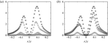
Figure 11. Plots of
 $({\it\Xi}/V_{t}^{2})\times 1000$
for the first POD mode (a) using
$({\it\Xi}/V_{t}^{2})\times 1000$
for the first POD mode (a) using
 $m=0$
(○), 1 (▫) and 2 (♢), and (b) using
$m=0$
(○), 1 (▫) and 2 (♢), and (b) using
 $m=0$
(○),
$m=0$
(○),
 $0+1$
(▫) and
$0+1$
(▫) and
 $0+1+2$
(♢) on a vortex slice at
$0+1+2$
(♢) on a vortex slice at
 ${\it\psi}=180^{\circ }$
. The original
${\it\psi}=180^{\circ }$
. The original
 $(\text{TKE}/V_{t}^{2})\times 1000$
(
$(\text{TKE}/V_{t}^{2})\times 1000$
(
6. Conclusions
The velocity fluctuations residing within two core radii from the centre of a vortex filament emanating from a single-bladed rotor were investigated using POD during hovering conditions. Upwards 75 % of the resolved energy from these turbulent motions was captured in the first (
 $n=1$
) POD mode alone for all the vortex ages studied. Within the first POD mode, the helical mode (
$n=1$
) POD mode alone for all the vortex ages studied. Within the first POD mode, the helical mode (
 $m=1$
) was found to dominate the energy spectrum, at all the vortex ages except at
$m=1$
) was found to dominate the energy spectrum, at all the vortex ages except at
 ${\it\psi}=45^{\circ }$
, followed by the axisymmetric (
${\it\psi}=45^{\circ }$
, followed by the axisymmetric (
 $m=0$
) and then the double helical (
$m=0$
) and then the double helical (
 $m=2$
) modes, where the azimuthal modes
$m=2$
) modes, where the azimuthal modes
 $m=1,2$
were shown to be associated with the elliptic instability. Near the blade tip at
$m=1,2$
were shown to be associated with the elliptic instability. Near the blade tip at
 ${\it\psi}=45^{\circ }$
, the axisymmetric mode was found to be as equally significant in energy as the helical mode due to the vortex roll-up process that occurs at inception. At higher vortex ages, the axisymmetric mode was found to manifest features similar to those of an axisymmetric swirling jet, which further enhances flow entrainment and diffusion mechanisms. Together, all the above large-scale motions were found to be responsible for the distinguishable asymmetries in the TKE inside the tip vortex.
${\it\psi}=45^{\circ }$
, the axisymmetric mode was found to be as equally significant in energy as the helical mode due to the vortex roll-up process that occurs at inception. At higher vortex ages, the axisymmetric mode was found to manifest features similar to those of an axisymmetric swirling jet, which further enhances flow entrainment and diffusion mechanisms. Together, all the above large-scale motions were found to be responsible for the distinguishable asymmetries in the TKE inside the tip vortex.
Acknowledgements
This work was supported by the Army/Navy/NASA Vertical Lift Research Center of Excellence (VLRCOE) led by the University of Maryland; Grant No. W911W6-11-2-0012. The authors also wish to acknowledge Christopher G. Cameron for his assistance with the PIV measurements.
Appendix A. Effects of vortex centring on the spatial modes
An important question that we seek to address is the effect of vortex centring on the spatial modes obtained by way of POD or harmonic decomposition. To address this matter, two approaches are considered. The first is evaluated in the main body of this paper, whereby the
 ${\it\Gamma}_{1}$
method is exercised. Because
${\it\Gamma}_{1}$
method is exercised. Because
 ${\it\Gamma}_{1}$
is an integral-based approach, it bypasses concerns regarding divergence-based schemes (such as the
${\it\Gamma}_{1}$
is an integral-based approach, it bypasses concerns regarding divergence-based schemes (such as the
 $Q$
,
$Q$
,
 ${\it\lambda}$
, vorticity, etc.), which might otherwise elevate noise. The condition that we wish to satisfy is that the in-plane turbulence goes to zero at the vortex centre. The
${\it\lambda}$
, vorticity, etc.), which might otherwise elevate noise. The condition that we wish to satisfy is that the in-plane turbulence goes to zero at the vortex centre. The
 ${\it\Gamma}_{1}$
approach achieves this, as is illustrated in figures 3 and 4. The issue however is whether having aligned the inner core region with the
${\it\Gamma}_{1}$
approach achieves this, as is illustrated in figures 3 and 4. The issue however is whether having aligned the inner core region with the
 ${\it\Gamma}_{1}$
approach causes the outer intermittent and turbulent regions to be smeared; it is postulated that the asymmetries in the TKE profiles are partially attributed to the misalignment of the outer turbulent structures. Therefore, a second approach is examined, which aims to align the outer turbulent structures by biasing the vortex centring technique with features associated with the outer portions of the vortex core. This is accomplished by aligning each vortex by way of its geometric centre. This geometric centre (hereafter referred to as GC) is determined based on the location of peak swirl velocity. Details of this technique are well documented by Mula et al. (Reference Mula, Stephenson, Tinney and Sirohi2013). The effect of using this kind of approach on the average vorticity and TKE is shown in figure 12 for the vortex filament at
${\it\Gamma}_{1}$
approach causes the outer intermittent and turbulent regions to be smeared; it is postulated that the asymmetries in the TKE profiles are partially attributed to the misalignment of the outer turbulent structures. Therefore, a second approach is examined, which aims to align the outer turbulent structures by biasing the vortex centring technique with features associated with the outer portions of the vortex core. This is accomplished by aligning each vortex by way of its geometric centre. This geometric centre (hereafter referred to as GC) is determined based on the location of peak swirl velocity. Details of this technique are well documented by Mula et al. (Reference Mula, Stephenson, Tinney and Sirohi2013). The effect of using this kind of approach on the average vorticity and TKE is shown in figure 12 for the vortex filament at
 ${\it\psi}=180^{\circ }$
vortex age. A cross-examination of figure 3(a,c) with figure 12(a,b) shows how the geometric centring approach has a minor effect on the mean vorticity field, while the TKE is characterized by a top-hat profile that is fairly uniform in azimuth. The values registered along the line
${\it\psi}=180^{\circ }$
vortex age. A cross-examination of figure 3(a,c) with figure 12(a,b) shows how the geometric centring approach has a minor effect on the mean vorticity field, while the TKE is characterized by a top-hat profile that is fairly uniform in azimuth. The values registered along the line
 ${\it\xi}$
in figure 12(b) are shown in figure 12(c) to further demonstrate the elevated turbulence levels at the vortex centre. So, while we have shown the differences in the statistical properties of the vortex due to the centring technique employed, the question that we will now focus on is the degree to which the centring technique affects the various modes associated with the inner, intermittently transitional and turbulent regions of the vortex.
${\it\xi}$
in figure 12(b) are shown in figure 12(c) to further demonstrate the elevated turbulence levels at the vortex centre. So, while we have shown the differences in the statistical properties of the vortex due to the centring technique employed, the question that we will now focus on is the degree to which the centring technique affects the various modes associated with the inner, intermittently transitional and turbulent regions of the vortex.

Figure 12. (a) Mean axial vorticity,
 ${\it\omega}_{z}/{\it\Omega}\times (-0.1)$
and (b)
${\it\omega}_{z}/{\it\Omega}\times (-0.1)$
and (b)
 $(\text{TKE}/V_{t}^{2})\times 10^{3}$
at
$(\text{TKE}/V_{t}^{2})\times 10^{3}$
at
 ${\it\psi}=180^{\circ }$
. (c) Swirl velocity,
${\it\psi}=180^{\circ }$
. (c) Swirl velocity,
 $(V_{{\it\Theta}}/V_{t})\times 10$
(▿), and
$(V_{{\it\Theta}}/V_{t})\times 10$
(▿), and
 $(\text{TKE}/V_{t}^{2})\times 10^{3}$
(
$(\text{TKE}/V_{t}^{2})\times 10^{3}$
(
 ${\it\xi}$
at
${\it\xi}$
at
 ${\it\psi}=180^{\circ }$
.
${\it\psi}=180^{\circ }$
.

Figure 13. Radial profile of the normalized energy of the Fourier-azimuthal modes of the TKE at
 ${\it\psi}=180^{\circ }$
using (a)
${\it\psi}=180^{\circ }$
using (a)
 ${\it\Gamma}_{1}$
and (b) GC methods for aligning the PIV snapshots. Locations of peak TKE (♢) and peak swirl velocity (○) are shown.
${\it\Gamma}_{1}$
and (b) GC methods for aligning the PIV snapshots. Locations of peak TKE (♢) and peak swirl velocity (○) are shown.

Figure 14. Radial profile of the normalized energy of the first three Fourier-azimuthal modes at (a)
 ${\it\psi}=180^{\circ }$
and (b)
${\it\psi}=180^{\circ }$
and (b)
 ${\it\psi}=495^{\circ }$
using the
${\it\psi}=495^{\circ }$
using the
 ${\it\Gamma}_{1}$
(filled symbols) and GC (open symbols) methods. The mean core radius using the
${\it\Gamma}_{1}$
(filled symbols) and GC (open symbols) methods. The mean core radius using the
 ${\it\Gamma}_{1}$
(solid line) and GC (dashed line) methods are also identified.
${\it\Gamma}_{1}$
(solid line) and GC (dashed line) methods are also identified.
In figure 13(a,b), the ensemble-averaged normalized Fourier-azimuthal mode spectrum (from (4.2)) associated with the
 ${\it\psi}=180^{\circ }$
vortex is shown for each radial position emanating from the vortex centre using the
${\it\psi}=180^{\circ }$
vortex is shown for each radial position emanating from the vortex centre using the
 ${\it\Gamma}_{1}$
and GC approach, respectively. This is being performed prior to decomposing the radial structure using POD. Thus, for a given Fourier-azimuthal mode, we wish to determine the radial position where its maximum energy resides, which is achieved by simply dividing
${\it\Gamma}_{1}$
and GC approach, respectively. This is being performed prior to decomposing the radial structure using POD. Thus, for a given Fourier-azimuthal mode, we wish to determine the radial position where its maximum energy resides, which is achieved by simply dividing
 $B_{ii}(r,{\it\psi};m)$
(in the Einstein notation) by its maximum value for a particular vortex age and mode number
$B_{ii}(r,{\it\psi};m)$
(in the Einstein notation) by its maximum value for a particular vortex age and mode number
 $m$
. While appreciable differences are observed in the statistical properties of the vortex (by comparing figures 3
a,c and 12
a,b), the higher Fourier-azimuthal modes illustrated in figure 13(a,b) appear to be unaffected by the centring technique chosen; the differences in the topographies between figure 13(a) and 13(b) are quite subtle. Additional lines have been added to this illustration identifying the location of peak swirl velocity and peak TKE. The only significant differences reside in the first few modes, which are re-illustrated for closer inspection in figure 14(a,b) for the
$m$
. While appreciable differences are observed in the statistical properties of the vortex (by comparing figures 3
a,c and 12
a,b), the higher Fourier-azimuthal modes illustrated in figure 13(a,b) appear to be unaffected by the centring technique chosen; the differences in the topographies between figure 13(a) and 13(b) are quite subtle. Additional lines have been added to this illustration identifying the location of peak swirl velocity and peak TKE. The only significant differences reside in the first few modes, which are re-illustrated for closer inspection in figure 14(a,b) for the
 $m=0,1$
and 2 modes. Here it is clearly shown how the geometric centring approach significantly changes the helical mode, which contributes predominantly to artificially elevated turbulence levels near the vortex centre. Subtle differences in the axisymmetric and double helical modes also appear, but only near or outside the vortex core radius. Hence, only the most unstable mode (
$m=0,1$
and 2 modes. Here it is clearly shown how the geometric centring approach significantly changes the helical mode, which contributes predominantly to artificially elevated turbulence levels near the vortex centre. Subtle differences in the axisymmetric and double helical modes also appear, but only near or outside the vortex core radius. Hence, only the most unstable mode (
 $m=1$
) associated with elliptic instabilities is significantly affected by the centring technique employed. Similar effects were observed for all other vortex ages.
$m=1$
) associated with elliptic instabilities is significantly affected by the centring technique employed. Similar effects were observed for all other vortex ages.
As for the radial structure of the vortex filament (using POD), the convergence of the Fourier-azimuthal modes in figure 15(a) for the first (
 $n=1$
) POD mode demonstrates how the geometric centring approach produces exactly the opposite behaviour from the
$n=1$
) POD mode demonstrates how the geometric centring approach produces exactly the opposite behaviour from the
 ${\it\Gamma}_{1}$
method where the axisymmetric mode and helical mode contributions are concerned. At early vortex ages (
${\it\Gamma}_{1}$
method where the axisymmetric mode and helical mode contributions are concerned. At early vortex ages (
 ${\it\psi}=45^{\circ }$
) the turbulent kinetic energy is governed almost entirely by the axisymmetric mode, which immediately changes to equal levels of contribution from the axisymmetric and helical modes at all other vortex ages. These findings are further studied in figure 15(b), where both the POD modes (integrated over all Fourier-azimuthal modes) and the Fourier-azimuthal modes (of the first POD mode) reflect similar overall rates of convergence, aside from the effects induced by the reshuffling of energy in the first few Fourier-azimuthal modes. In particular, the POD functional basis for the vortex turbulence is shown to be compatible with the
${\it\psi}=45^{\circ }$
) the turbulent kinetic energy is governed almost entirely by the axisymmetric mode, which immediately changes to equal levels of contribution from the axisymmetric and helical modes at all other vortex ages. These findings are further studied in figure 15(b), where both the POD modes (integrated over all Fourier-azimuthal modes) and the Fourier-azimuthal modes (of the first POD mode) reflect similar overall rates of convergence, aside from the effects induced by the reshuffling of energy in the first few Fourier-azimuthal modes. In particular, the POD functional basis for the vortex turbulence is shown to be compatible with the
 $k^{-5/3}$
inertial range spectrum that is expected even of inhomogeneous turbulence (Moser Reference Moser1994).
$k^{-5/3}$
inertial range spectrum that is expected even of inhomogeneous turbulence (Moser Reference Moser1994).

Figure 15. (a) Fourier mode energy spectra of the first (
 $n=1$
) POD mode for
$n=1$
) POD mode for
 $m=0$
(○), 1 (
$m=0$
(○), 1 (
 ${\it\psi}=180^{\circ }$
.
${\it\psi}=180^{\circ }$
.
Where the POD spatial structure is concerned (effectively
 ${\it\Phi}_{i}^{(n)}(r,{\it\psi};m)$
), figure 16 shows how the first six (
${\it\Phi}_{i}^{(n)}(r,{\it\psi};m)$
), figure 16 shows how the first six (
 $m=0{-}5$
) Fourier-azimuthal modes associated with the first POD mode contribute to the resolved TKE along the radial coordinate at
$m=0{-}5$
) Fourier-azimuthal modes associated with the first POD mode contribute to the resolved TKE along the radial coordinate at
 ${\it\psi}=180^{\circ }$
. These profiles, normalized by their maximum values, are computed using the standard expression
${\it\psi}=180^{\circ }$
. These profiles, normalized by their maximum values, are computed using the standard expression
 $$\begin{eqnarray}\mathfrak{B}_{ii}^{(1)}(r,{\it\psi};m)={\it\Lambda}^{1}({\it\psi};m)\,{\it\Phi}_{i}^{(1)}(r,{\it\psi};m)\,{\it\Phi}_{i}^{(1)\ast }(r,{\it\psi};m),\end{eqnarray}$$
with subscripts written in the Einstein notation. Contrary to figure 14, the axisymmetric and double helical modes associated with the first POD mode are shown in figure 16 to be significantly affected by the choice of the centring technique. That is, the
 $m=0$
and
$m=0$
and
 $m=2$
spatial structures are located further outwards radially from the vortex centre using the
$m=2$
spatial structures are located further outwards radially from the vortex centre using the
 ${\it\Gamma}_{1}$
method relative to the GC method. It is also interesting to see how Fourier-azimuthal mode numbers
${\it\Gamma}_{1}$
method relative to the GC method. It is also interesting to see how Fourier-azimuthal mode numbers
 $m=3$
, 4 and 5 peak at further distances, where the turbulent eddies are expected to mix and eventually diffuse their energy to the outer mean flow. This illustrates the exchange of energy between the larger scales (residing near the vortex core) and the smaller scales (residing further away in the outer peripheries of the vortex), and is complementary to the findings displayed in figure 13.
$m=3$
, 4 and 5 peak at further distances, where the turbulent eddies are expected to mix and eventually diffuse their energy to the outer mean flow. This illustrates the exchange of energy between the larger scales (residing near the vortex core) and the smaller scales (residing further away in the outer peripheries of the vortex), and is complementary to the findings displayed in figure 13.

Figure 16. Radial profile of the normalized energy at
 ${\it\psi}=180^{\circ }$
for the first six Fourier-azimuthal modes associated with the first POD mode using the
${\it\psi}=180^{\circ }$
for the first six Fourier-azimuthal modes associated with the first POD mode using the
 ${\it\Gamma}_{1}$
(filled symbols) and GC (open symbols) methods.
${\it\Gamma}_{1}$
(filled symbols) and GC (open symbols) methods.


