


1. Introduction
Surfactant-stabilized oil–water emulsions are ubiquitous, and have been studied for many decades (Prosser & Franses Reference Prosser and Franses2001). More recently, interest has turned to nano-emulsions, for which the oil droplet size is  ${\sim } 100\text {--}600$ nm (Bouchemal et al. Reference Bouchemal, Briancon, Perrier and Fessi2004). The large surface-to-volume ratio is advantageous for purifying and releasing oil-soluble drugs (Gupta et al. Reference Gupta, Eral, Hatton and Doyle2016; Hashemnejad et al. Reference Hashemnejad, Badruddoza, Zarket, Ricardo Castaneda and Doyle2019), and there has been a resurgence in efforts to understand the interfacial surface charge, which plays a pivotal role in maintaining a small drop size: by providing an electro-steric barrier to the thermodynamic tendency for coalescence (Hunter Reference Hunter2001). Whereas surface-charge density has conventionally been ‘measured’ using microelectrophoresis (i.e. the drop velocity induced by a steady electric field), such measurements have provoked controversy. This is because the conversion of a velocity to surface charge requires a model, and such models are especially complex when the surface charge is high (Russel, Saville & Showalter Reference Russel, Saville and Showalter1989)– as seems to be the case for charged surfactants, such as sodium dodecyl sulphate (SDS) (Borwankar & Wasan Reference Borwankar and Wasan1988; Hunter & O'Brien Reference Hunter and O'Brien1997). Another indirect means of assessing the surface-charge density is to measure the interfacial surface tension, and convert this to a surface-charge density by invoking an adsorption isotherm. While this seems to furnish a robust interpretation of the surface tension (Borwankar & Wasan Reference Borwankar and Wasan1988), the accompanying surface charge densities are very high (compact monolayer coverage), thus casting doubt on the isotherms (Kralchevsky et al. Reference Kralchevsky, Danov, Broze and Mehreteab1999) or the validity of electrokinetic models (Yang et al. Reference Yang, Wu, Chen and Gan2017).
To help circumvent the challenges of interpreting electrophoresis with electrokinetic theory, de Aguiar et al. (Reference de Aguiar, de Beer, Strader and Roke2010) developed a novel vibrational sum frequency scattering experiment to determine the surface charge density. In this study, and others that follow it (Zdrali et al. Reference Zdrali, Chen, Okur, Wilkins and Roke2017, Reference Zdrali, Etienne, Smolentsev, Amstad and Roke2019), the experiments suggest that the interfacial charge of nano-drops is anomalously low as compared to their macro-scale counterparts. One explanation hinges on a weakly charged oil phase promoting strong repulsive electrostatic interactions between adsorbed surfactant ions (Zdrali et al. Reference Zdrali, Chen, Okur, Wilkins and Roke2017). On the other hand, earlier electrokinetic studies of similar emulsions suggest much higher surface charge densities (Barchini & Saville Reference Barchini and Saville1996; Hunter & O'Brien Reference Hunter and O'Brien1997; Djerdjev & Beattie Reference Djerdjev and Beattie2008; Kong, Beattie & Hunter Reference Kong, Beattie and Hunter2001), but no studies have unified the electrokinetic and adsorption-isotherm derived interfacial charges.
Upon closer inspection, questions emerge regarding the electrokinetic ‘validation’ of the vibrational sum frequency scattering undertaken by de Aguiar et al. (Reference de Aguiar, de Beer, Strader and Roke2010). These authors reported the  $\zeta$-potential furnished by a commercial electrophoretic light-scattering instrument, also reporting (from dynamic light scattering undertaken on the same instrument) a number-averaged drop radius
  $a \approx 83 \pm 10$ nm, implicitly inferring that the scaled drop radius
  $\kappa a \gg 1$ (radius
  $a$ and Debye length
  $\kappa ^{-1}$). Under these conditions, the measured mobility is often considered independent of the size, so the authors implicitly reported a ‘Smoluchowski’
  $\zeta$-potential:
  $\zeta _S \approx - 116$ mV.
However, if we estimate the ionic strength based on the SDS concentration  ${\approx }8$ mM (there was no added salt), then we find
  $\kappa ^{-1} \approx 3.4$ nm, furnishing
  $\kappa a \approx 24$. Thus, the diffuse layer is indeed thin, but is it thin enough? The dimensionless mobility from the reported
  $\zeta$-potential is
  $M^* = -3 \zeta _S e / (2 k_B T) \approx - 7.0$ (
 $k_B T / e \approx 25$ mV is the thermal energy divided by the fundamental charge, k B is Boltzmann's constant, and T is the absolute temperature). Therefore, if we check the Smoluchowski interpretation, by comparing it with the standard electrokinetic model (O'Brien & White Reference O'Brien and White1978), then we discover that there is no value of
  $\kappa a \lesssim 140$ that can furnish such a high mobility. If, instead, we attempt to evaluate the
  $\zeta$-potential at
  $\kappa a \approx 140$ (e.g. allowing for a much larger mobility-averaged drop radius), then the standard electrokinetic model infers a considerably larger surface potential:
  $\zeta \approx - 7 k_B T / e \approx -175$ mV, and, therefore, a much higher surface-charge density than suggested by de Aguiar et al. (Reference de Aguiar, de Beer, Strader and Roke2010). Thus, while the conclusions drawn by de Aguiar et al. (Reference de Aguiar, de Beer, Strader and Roke2010) from their Smoluchowski
  $\zeta$-potential seem reasonable, the validity of the Smoluchowski formula, which is an approximation of the standard-electrokinetic model, is questionable; and the averaged drop size and mobility are incompatible with the standard electrokinetic model.
Note that the foregoing electrokinetic models are for rigid spheres, which drops are not (Wuzhang et al. Reference Wuzhang, Song, Sun, Pan and Li2015). Nevertheless, Marangoni forces can be invoked to justify an immobile/rigid interface, at least at low/zero frequency (Baygents & Saville Reference Baygents and Saville1991). Moreover, according to
Hunter (Reference Hunter2001, equation (8.8.12)), the Dukhin numbers  $\lambda \approx \exp {[|z e \zeta | / (k_B T)] / \kappa a}$ that accompany the Smoluchowski interpretations above are not much less than one, whereas scaling analysis requires
  $\lambda \ll 1$ to justify the underlying Smoluchowski-slip velocity model. For the drops in the electrophoresis experiments of de Aguiar et al. (Reference de Aguiar, de Beer, Strader and Roke2010),
  $\lambda \approx 0.42$ when
  $(|\zeta |, \kappa a) = (116\ \mbox {mV}, 24)$, whereas
  $\lambda \approx 0.24$ when
  $(|\zeta |,\kappa a) = (175\ \mbox {mV}, 140)$. Accordingly, charge-density perturbations inside the diffuse layer may cause the fluid dynamics to depart from the Smoluchowski-slip model (Hunter Reference Hunter2001).
To address the high surface charge (and accompanying high surface conductivity) and fluid characteristics of nano-drops in dynamic electrophoretic mobility experiments (O'Brien Reference O'Brien1988, Reference O'Brien1990), Hill & Afuwape (Reference Hill and Afuwape2020) recently proposed a thin-double-layer model for the dynamic mobility, valid at high frequencies for which there is no time for diffusive ion transport. They assumed that the adsorbed surfactant is bound to the interface while the drop is subjected to an oscillatory electric field. Electroosmotic flow in the diffuse layer was assumed to be driven by an electrical body force that is equal to the product of the equilibrium charge density in the diffuse layer and an electric field that is calculated without any perturbation to the equilibrium charge density (Smoluchowski-slip approximation at vanishing Dukhin number). Moreover, the region outside the diffuse layer was assumed to remain uncharged, thus neglecting charge transfer between the interface, diffuse layer and bulk (pseudo-binary) electrolyte. These simplifications furnished a closed-form solution for when the diffuse layer is occupied solely by ( $\textrm {Na}^+$) counterions of the adsorbed (
 $\textrm {DS}^-$) surfactant, thus limiting the accuracy to highly charged interfaces, but subject to a small Dukhin number. The model revealed fluid-like interfacial characteristics at the MHz frequencies at which dynamic electrophoretic mobility experiments are undertaken (via the electrokinetic sonic amplitude, ESA) (O'Brien, Cannon & Rowlands Reference O'Brien, Cannon and Rowlands1995).
The ESA is an acoustic pressure arising from electric-field-induced particle motion (dynamic electrophoresis) in a dispersion. Experiments are undertaken in at frequencies  $\omega / (2 {\rm \pi}) = 1\text {--}20$ MHz so that the sound wavelength is large compared to the particle size, and small compared to the sample. Momentum transfer arising from the finite particle velocity
  $\boldsymbol {V} = M(\omega ) \boldsymbol {E}$ (
 $M(\omega )$ is the dynamic mobility,
  $\boldsymbol {E}$ is the applied electric field) generates the pressure, even though the particle displacement
  $\boldsymbol {X} \sim \boldsymbol {V} / \omega$ (and deformation) is vanishingly small at such frequencies (O'Brien Reference O'Brien1988, Reference O'Brien1990).
Combining their electrokinetic model with an isotherm from surface-tension measurements on macro-scale (pendent) drops, the ‘unified’ model of Hill & Afuwape (Reference Hill and Afuwape2020) provided a compelling (but incomplete) interpretation of dynamic mobility spectra (magnitude and phase angle): owing to the high surface-charge densities, the Dukhin numbers are readily greater than one, again casting doubt on the Smoluchowski-slip approximation.
The present computational study removes all the foregoing simplifying approximations. This provides a theoretical interpretation for (non-conducting) drops of all sizes and charge, in electrolytes with multiple (fully ionized) electrolyte ions (charged surfactant and added salt), also providing guidance on how low  $\kappa a \gg 1$ must be to apply the thin-double-layer, high
  $\zeta$-potential model of Hill & Afuwape (Reference Hill and Afuwape2020). Without limits on the drop size, the model enables rigorous averaging for emulsions that are, in practice, polydisperse. This may help to resolve ambiguities arising from complementary diagnostic characterizations based on number, area or volume averaging. For example, drop sizes from dynamic light scattering may be reported as intensity-, volume- or number-weighted averages, whereas dynamic electrophoretic mobilities from the ESA are expected to reflect a volume/mass averaging (O'Brien et al. Reference O'Brien, Cannon and Rowlands1995). Moreover, electrical conductivity measurements on dispersions (Hollingsworth & Saville Reference Hollingsworth and Saville2003) may reflect an area averaging (charge density proportional to interfacial area) and volume averaging (dipole polarization proportional to volume), perhaps depending on the frequency. It is therefore important to quantify how the dynamic mobility and polarizability depend on drop size. The model presented here furnishes the dynamic mobility (magnitude and phase spectra), as well as the dynamic polarizability, which is readily converted to a complex-conductivity increment (Delacey & White Reference Delacey and White1981).
As detailed in the next § 2, the model seeks to capture interfacial dynamics arising from exchange of surfactant between the interface and the immediately adjacent electrolyte, and Marangoni stresses arising from interfacial surfactant concentration gradients; with full account of nonlinear electrostatics, and ion transport by electro-migration, diffusion and advection – albeit in the so-called weak-field limit where the dynamic fields are linear perturbations to an equilibrium base state. Although the model is developed with SDS-stabilized oil-in-water emulsions as an example, it may be applied to bubbles (Booth Reference Booth1951; Baygents & Saville Reference Baygents and Saville1991) for which there has been recent interest in electrophoresis beyond the weak-field limit (Schnitzer, Frankel & Yariv Reference Schnitzer, Frankel and Yariv2014). Although not undertaken here, the present model can, in principle, be extended to emulsions in which a conducting (e.g. aqueous) phase is dispersed in a non-conducting (e.g. oil) phase. Such systems are more challenging to study from an experimental perspective, since the continuous phase is typically required to have a sufficient electrical conductivity (achieved by the addition of electrolyte).
In the present study, special consideration is given to the interface (§ 2.2), coupling its dynamics (surfactant transport, and electrical, Marangoni and hydrodynamic stresses) to that of the internal fluid (§ 2.1) and external electrolyte (§ 2.3) when subjected to a weak, oscillatory electric field. After detailing how the internal and interfacial dynamics is coupled to the external electrolyte (§ 3), the results are presented (§ 4), using parameters for SDS-stabilized oil-in-water emulsions. These establish a lower limit on the drop radius for the thin-double-layer model of Hill & Afuwape (Reference Hill and Afuwape2020), also explicitly addressing the drop size and mobilities reported by de Aguiar et al. (Reference de Aguiar, de Beer, Strader and Roke2010). Next, more general aspects of the model are explored (§ 5), varying parameters (e.g. viscosity ratio, Marangoni parameter, kinetic-exchange coefficients) that influence the interfacial mobility and surfactant exchange. Particular attention is given to understanding the electrical polarization, its dependence on particle size and interfacial mobility, and how it couples to electroosmotic flow.
2. Theory
A single drop (or bubble) in an unbounded electrolyte is assumed to be spherical and non-conducting. Drops and bubbles are distinguished by their internal viscosity and density with respect to the outer, surfactant-containing electrolyte. The spherical shape is a consequence of the equilibrium surface tension dominating the radial interfacial momentum balance (Taylor & Acrivos Reference Taylor and Acrivos1964). Although the internal viscosity and density are arbitrary, the vanishing conductivity implicitly requires this fluid to be a non-ionized gas (e.g. air) or non-polar liquid (e.g. oil). The absence of charge enables the internal flow and electric field to be prescribed by tractable analytical formulas, for which unknown integration constants are prescribed by coupling the interior flow to an intricate numerical solution for the exterior domain. The external electrolyte contains an ionic (assumed completely dissociated) surfactant, which adsorbs to the interface, and added salt; thus forming an equilibrium diffuse double layer with an accompanying surface-charge density  $\sigma ^0$ and surface potential
  $\zeta$ (Russel et al. Reference Russel, Saville and Showalter1989; Hunter Reference Hunter2001). Then, with the application of a uniform, oscillatory electric field
  $\boldsymbol {E} \,\textrm {e}^{- \textrm {i} \omega t}$ (real part thereof), electrical forces due to charge at the interface and in the diffuse layer induce an oscillatory particle velocity
  $\boldsymbol {V} \,\textrm {e}^{- \textrm {i} \omega t}$.
Mathematically, fluctuations in the internal, interface and external fluid velocities, ion and surfactant concentrations and electro-static potential are coupled to the particle motion by the linear superposition of two simpler problems: the application of an electric field to a stationary drop in a stationary electrolyte ( $E$-problem), and the application of a uniform flow (velocity
  $\boldsymbol {U} \,\textrm {e}^{- \textrm {i} \omega t}$, in the absence of an electric field) to a stationary drop (
 $U$-problem). The forces on the drop for these two problems are then superposed to satisfy the particle equation of motion, thus furnishing the complex-valued coefficient of proportionality between the particle velocity and electric field, which is customarily termed the dynamic electrophoretic mobility,
  $M(\omega )$ with
  $\boldsymbol {V} = M(\omega ) \boldsymbol {E}$.
Note that the  $U$- and
  $E$-problems will be drawn upon to help elucidate pertinent details of the highly coupled physical processes taking place. Section 2.1 recapitulates the internal dynamics (velocity and electric field) as set out by Hill & Afuwape (Reference Hill and Afuwape2020). Section 2.2 details the interface, including its equilibrium thermodynamics and dynamics. Section 2.3 presents essential features of the external thermodynamics and dynamics, avoiding details, since the model is the same as addressed in earlier well-known computational studies, e.g. as pioneered for rigid spheres by Delacey & White (Reference Delacey and White1981) (dielectric response) and Mangelsdorf & White (Reference Mangelsdorf and White1992) (dynamic mobility). Section 3 (and appendix A) details how the internal, interfacial, and external regions are coupled in an efficient numerical method that solves this notoriously stiff numerical problem over a wide range of the parameter space (Hill, Saville & Russel Reference Hill, Saville and Russel2003). This section also sets out notation (and non-dimensionalization), including the superposition of the
  $U$- and
  $E$-problems. Readers who are not concerned with theoretical and computation details may skip to the results § 4, perhaps referring back to §§ 2.1–3 for relevant notation.
2.1. Inside the drop
Inside the drop, which is assumed to be a Newtonian, non-conducting, dielectric fluid, we have mass conservation, momentum conservation and Laplace equations
 \begin{equation} - \textrm{i} \omega \rho_i \boldsymbol{u} = -\boldsymbol{\nabla}{p} + \eta_i \nabla^2 \boldsymbol{u}\quad \mbox{with}\ \boldsymbol{\nabla} \boldsymbol{\cdot} \boldsymbol{u} = 0 \end{equation}
and
 \begin{equation} \nabla^2 \psi = 0, \end{equation}
where  $\rho _i$ and
  $\eta _i$ are the density and shear viscosity for ‘inside’ the drop. The velocity
  $\boldsymbol {u}$, pressure
  $p$ and electrostatic potential
  $\psi$ (and all other independent variables) will be taken to have harmonic time dependence via
  $\textrm {e}^{-\textrm {i} \omega t}$, where
  $\omega$ is the angular frequency. Note that the nonlinear inertial term is neglected, requiring a small Reynolds number
  ${Re} = u_c a \rho _i / \eta _i$, where
  $a$ is the drop radius and the characteristic electrophoretic velocity
  $u_c = (k_B T / e) \epsilon _o \epsilon _0 / (\eta _o a)$ (Russel et al. Reference Russel, Saville and Showalter1989) with
  $k_B T / e \sim 25$ mV the thermal potential and
  $\epsilon _o \epsilon _0$ the dielectric permittivity of the external solution.
For a drop that is taken to be spherical, the radial velocity (in the frame moving with the drop) of the interface vanishes. Hill & Afuwape (Reference Hill and Afuwape2020) have shown that the tangential velocity and traction at the interface (with inward unit normal  $- \boldsymbol {e}_r$) can be written
 \begin{equation} \boldsymbol{u}_\theta(r = a_-) = c_1 a V_i(\varOmega_i a^2)\,\textrm{e}^{-\textrm{i} \omega t} \boldsymbol{X} \boldsymbol{\cdot} \boldsymbol{e}_\theta \boldsymbol{e}_\theta, \end{equation}
and
 \begin{equation} \boldsymbol{t}_\theta(r = a_-) = - \eta_i c_1 T_i(\varOmega_i a^2) \,\textrm{e}^{-\textrm{i} \omega t} \boldsymbol{X} \boldsymbol{\cdot} \boldsymbol{e}_\theta \boldsymbol{e}_\theta, \end{equation}
where
 \begin{align} \varOmega_i^2 a^4 V_i(\varOmega_i a^2) &= \left(3-\textrm{i} \varOmega_i a^2\right) \sin \left[(1+\textrm{i}) \sqrt{\varOmega_i/2} a\right]\nonumber\\ &\quad -3 (1+\textrm{i}) \sqrt{\varOmega_i /2} a \cos \left[(1+\textrm{i}) \sqrt{\varOmega_i /2 } a\right] \end{align}
and
 \begin{align} \varOmega_i^2 a^4 T_i(\varOmega_i a^2) &= \left[6 (1+\textrm{i}) \sqrt{\varOmega_i/2} a - (i-\textrm{1}) 2^{-1/2} \varOmega_i^{3/2} a^3\right] \cos \left[(1+\textrm{i}) \sqrt{\varOmega_i/2} a\right] \nonumber\\ &\quad + \left(3 \textrm{i} \varOmega_i a^2 - 6\right) \sin \left[(1+\textrm{i}) \sqrt{\varOmega_i/2} a\right] \end{align}
with  $\varOmega _i = \omega \rho _i / \eta _i$ (square of the reciprocal viscous penetration depth). Moreover, the electrostatic potential
 \begin{equation} \psi(\boldsymbol{x}, t) = \psi^0 + \psi'(\boldsymbol{x}) \,\textrm{e}^{-\textrm{i} \omega t} = \psi^0 + [\hat{\psi}(r = a) (r/a) - r (E/X)] \,\textrm{e}^{-\textrm{i} \omega t} \boldsymbol{X} \boldsymbol{\cdot} \boldsymbol{e}_r \quad\mbox{for}\ r < a, \end{equation}
where  $\psi ^0$ and
  $\hat {\psi }(r = a)$ are constants. Thus, the dynamics inside the drop is determined to two unknown scalar integration constants:
  $c_1$ and
  $\hat {\psi }(r = a)$, which will be determined by coupling the internal dynamics to the interface and external electrolyte.
2.2. Interface
Taking the interface to be infinitesimally thin, a conservation equation for any adsorbed species with surface number density
 \begin{equation} c(\boldsymbol{x}, t) = c^0 + \textrm{e}^{-\textrm{i} \omega t} c'(\boldsymbol{x}) \end{equation}
may be written
 \begin{equation} - \textrm{i} \omega c' = -\boldsymbol{\nabla}_s \boldsymbol{\cdot} \left( - D \boldsymbol{\nabla}_s c' - \boldsymbol{\nabla}_s {\psi'} z e c^0 \frac{D}{k_B T} + \boldsymbol{u}_\theta c^0 \right) + k_a n'(r= a) - k_d c' , \end{equation}
where  $\boldsymbol {\nabla }_s$ is the surface gradient operator and
  $\boldsymbol {u}_\theta$ is the interfacial (tangential) velocity. The tangential flux comprises lateral diffusion (diffusivity
  $D$), electro-migration (charge
  $z e$), and advection terms. Note that the flux is linearized for perturbations (primed quantities) about the equilibrium state (superscripts ‘0’). The ‘source’ terms with adsorption and desorption coefficients
  $k_a$ and
  $k_d$ capture exchange between the interface and the immediately adjacent external fluid where the concentration is
 \begin{equation} n(\boldsymbol{x},t) = n^0(r) + \textrm{e}^{- \textrm{i} \omega t}n'(\boldsymbol{x}) \end{equation}
with
 \begin{equation} n^0(r) = n^\infty \exp({-\psi^0(r) z e / (k_B T)}) \end{equation}
the equilibrium concentration. Note that  $n^\infty$ is the bulk concentration of the adsorbing species, and
  $\psi ^0(r)$ is the equilibrium electrostatic potential.
At equilibrium,
 \begin{equation} k_a n^0(r = a) = k_d c^0 = k_a n^\infty \exp({-\psi^0(r=a) z e / (k_B T)}), \end{equation}
so the ratio of the exchange coefficients is related to the equilibrium adsorption isotherm  $c^0 = \hat {\varGamma }(n^\infty ,\ldots .)$. Thus, with knowledge of the equilibrium isotherm, there is only one independent kinetic-exchange coefficient. Their ratio
 \begin{equation} \frac{k_a}{k_d} = \frac{\hat{\varGamma}(n^\infty,\ldots.)}{n^\infty \exp({- \psi^0(r=a) z e / (k_B T)})} \end{equation}
has the dimension of length:  $k_a$ has dimensions of velocity, whereas
  $k_d$ has the dimension of reciprocal time, interpreted as the frequency at which adsorbed molecules transfer from the interface to the immediately adjacent (external) fluid. For example, for SDS with
  $\hat {\varGamma } = c^0 \sim 1\ \textrm {nm}^{-2}$,
  $n^\infty \sim 1\ \mbox {mM} \sim 10^{-3}\ \mbox {nm}^{-3}$ and
  $\exp ({- \psi ^0(r=a) z e / (k_B T)}) \sim \textrm {e}^{-8}$, we find
  $k_a / k_d \sim 10^6$ nm. Thus, if we estimate
  $k_a$ based on the diffusion velocity
  $k_a \sim \kappa D_1 \sim 0.01\ \textrm {m}\,\textrm {s}^{-1}$, where
  $\kappa ^{-1}$ is the Debye length and
  $D_1 \sim 10^{-10}\ \textrm {m}^2\,\textrm {s}^{-1}$ is the surfactant diffusivity in the aqueous electrolyte, then
 \begin{equation} k_d \sim 10\ \mbox{Hz}. \end{equation}
This is significantly smaller than an estimate based on the product of a frequency factor  $A = k_B T / h$ (Planck's constant
  $h \approx 6.6 \times 10^{-34}\ \textrm {J}\,\textrm {s}$) and a Boltzmann desorption probability
  $\exp ({{\rm \Delta} \epsilon / (k_B T)})$, where the adsorption enthalpy
  ${\rm \Delta} \epsilon \approx -19 k_B T$ from the isotherm of Hill & Afuwape (Reference Hill and Afuwape2020), which furnishes
 \begin{equation} k_d \sim \frac{k_B T}{h} \exp({{\rm \Delta} \epsilon / (k_B T)}) \sim 10\ \mbox{kHz}. \end{equation}
Nevertheless, both estimates suggest that, at the MHz forcing of an electroacoustic experiment, the adsorbed  $\textrm {DS}^{-}$ is expected to behave as if it is irreversibly bound to the interface, as assumed by Hill & Afuwape (Reference Hill and Afuwape2020) who implicitly set
  $k_a = k_d = 0$ based on ‘kinetic rates’ being much smaller than
  ${\sim }1$ MHz. Here, the kinetic rate implied by Hill & Afuwape (Reference Hill and Afuwape2020) is more precisely
 \begin{equation} k_d \sim \kappa D_1 \frac{n^\infty \exp({- \psi^0(r=a) z e / (k_B T)})}{\hat{\varGamma}(n^\infty,\ldots.)}. \end{equation}
Table 1 provides a summary of data calculated from the isotherm of Hill & Afuwape (Reference Hill and Afuwape2020) for SDS adsorbing at an oil–water interface with the concentration of added NaCl in the aqueous phase fixed at  $I_s = 1$ mM. As suggested by the scaling analysis above, the dimensionless group
  $\kappa k_a / k_d$ is very large, spanning in the range
  $10^5\text {--}10^6$. Similar calculations show that other added-salt concentrations do not significantly change this ratio. As expected, its large value reflects the strong binding of
  $\textrm {DS}^{-}$ ions to the oil phase (smallness of
  $k_d$). Nevertheless, by developing the present electrokinetic model to handle kinetic- and diffusion-limited exchange dynamics (i.e. finite
  $k_d$ and
  $k_a$), it bridges the diffusion-limited regime of Baygents & Saville (Reference Baygents and Saville1991), and the kinetic-exchange-limited range of Hill & Afuwape (Reference Hill and Afuwape2020). The model may therefore be applied to other adsorbing species, or to SDS-like systems at much lower frequencies, e.g. for emulsion synthesis and mixing processes.
Table 1. Isotherm calculations for SDS (below the critical micelle concentration) at the hexadecane–water interface: added-salt (NaCl) concentration  $I_s = 1$ mM, oil–water surface tension (without surfactant)
  $\gamma (0,0) = 47\ \textrm {mN}\,\textrm {m}^{-1}$. Bulk SDS concentration
  $c_\infty$, equilibrium
  $\textrm {DS}^-$ surface concentration
  $c^0$.

In addition to the forgoing adsorbed-species conservation equation, we have an interfacial tangential momentum conservation equation (with zero interfacial inertia)
 \begin{equation} \boldsymbol{t}_\theta(r = a_-) + \boldsymbol{t}_\theta(r = a_+) - \gamma^0 \beta \boldsymbol{\nabla}_s{c'} - c^0 z e \boldsymbol{\nabla}_s{\psi'} = 0, \end{equation}
where  $\boldsymbol {t}_\theta (r = a_-)$ and
  $\boldsymbol {t}_\theta (r = a_+)$ are the (tangential) viscous tractions acting on the inside and outside of the interface (outward unit normals
  $-\boldsymbol {e}_r$ and
  $\boldsymbol {e}_r$), e.g.
 \begin{equation} \boldsymbol{t}_\theta(r = a_+) = \{- p \boldsymbol{I} + \eta_o [\boldsymbol{\nabla}{\boldsymbol{u}} + (\boldsymbol{\nabla}{\boldsymbol{u}})^\textrm{T}\} \boldsymbol{\cdot} \boldsymbol{e}_r \boldsymbol{\cdot} \boldsymbol{e}_\theta \boldsymbol{e}_\theta. \end{equation}
Moreover,  $- \gamma ^0 \beta \boldsymbol {\nabla }_s{c'}$ is the resultant interfacial tension/Marangoni stress (
 $\gamma ^0 \beta = \partial \gamma ^0 / \partial c^0|_{c^0}$ with
  $\gamma ^0$ the equilibrium interfacial tension), and
  $- c^0 z e \boldsymbol {\nabla }_s{\psi '}$ is the resultant (tangential) electrical/Maxwell stress.
Finally, we have Gauss's law at the interface
 \begin{equation} \epsilon_i \epsilon_0 \boldsymbol{\nabla} \psi' \boldsymbol{\cdot} \boldsymbol{e}_r | _{r = a_-} - \epsilon_o \epsilon_0 \boldsymbol{\nabla} \psi' \boldsymbol{\cdot} \boldsymbol{e}_r | _{r = a_+} = \sigma' = z e c', \end{equation}
where the interfacial-charge density is
 \begin{equation} \sigma(\boldsymbol{x},t) = \sigma^0 + \textrm{e}^{-\textrm{i} \omega t} \sigma'(\boldsymbol{x}) = \sigma^0 + z e \,\textrm{e}^{-\textrm{i} \omega t} c'(\boldsymbol{x}), \end{equation}
with
 \begin{equation} \sigma^0 = - \epsilon_o \epsilon_0 \left. \frac{\partial \psi^0}{\partial r} \right|_{r = a_+} \end{equation}
the equilibrium interfacial-charge density ( $\sigma ^0 = z e c^0$ for a single adsorbing species), e.g. as furnished by an equilibrium adsorption isotherm or equilibrium surface potential
  $\zeta = \psi ^0(r = a)$.
2.3. Outside the drop
Outside the drop we have differential conservation equations for  $N$ ionic species, and fluid mass and momentum. With Gauss's law, these are termed the standard electrokinetic model, and need not be reproduced here. Note, however, that these equations are solved (for
  $r > a$) in terms of the following independent variables (ion concentrations, electrostatic potential and fluid velocity):
 \begin{gather} n_i(\boldsymbol{x},t) = n^0_i(r) + \hat{n}_i(r) \,\textrm{e}^{-\textrm{i} \omega t} \boldsymbol{X} \boldsymbol{\cdot} \boldsymbol{e}_r \quad (i = 1,\ldots, N), \end{gather}
 \begin{gather}\psi(\boldsymbol{x},t) = \psi^0(r) - r \,\textrm{e}^{-\textrm{i} \omega t} \boldsymbol{E} \boldsymbol{\cdot} \boldsymbol{e}_r + \hat{\psi}(r) \,\textrm{e}^{-\textrm{i} \omega t} \boldsymbol{X} \boldsymbol{\cdot} \boldsymbol{e}_r , \end{gather}
and (Hill et al. Reference Hill, Saville and Russel2003)
 \begin{equation} \boldsymbol{u}(\boldsymbol{x},t) = \textrm{e}^{-\textrm{i} \omega t} \boldsymbol{U} + \boldsymbol{\nabla} \times \boldsymbol{\nabla} \times [h(r) \, \textrm{e}^{-\textrm{i}\omega t} \boldsymbol{X} \boldsymbol{\cdot} \boldsymbol{e}_{r}]. \end{equation}
One may also write (Hill & Afuwape Reference Hill and Afuwape2020)
 \begin{align} \boldsymbol{u}(\boldsymbol{x},t) &= \boldsymbol{\nabla} \times [\,f(r) \,\textrm{e}^{-\textrm{i} \omega t} \boldsymbol{X} \times \boldsymbol{e}_{r}] \nonumber\\ &= (\,f_{r} +f r^{-1}) \,\textrm{e}^{-\textrm{i} \omega t} \boldsymbol{X} +(-f_{r} + f r^{-1})\, \textrm{e}^{-\textrm{i} \omega t} \boldsymbol{X} \boldsymbol{\cdot} \boldsymbol{e}_{r} \boldsymbol{e}_{r}, \end{align}
so
 \begin{equation} f = r U / (2 X) - h_r, \quad f_{r} = U / (2 X) - h_{rr},\quad \mbox{and}\quad f_{rr} = - h_{r,rr} = - g, \end{equation}
where  $g \equiv h_{r,rr}$ is an auxiliary variable to avoid derivatives in the numerical solution that are higher than second order.
To couple the  $N$ ion-conservation equations in the standard electrokinetic model to the interface, their (Nernst–Planck) fluxes at the interface must satisfy
 \begin{equation} \left(- D_i \boldsymbol{\nabla} n'_i - \boldsymbol{\nabla} {\psi'} z_i e n_i^0 \frac{D_i}{k_B T} + n_i^0 \boldsymbol{u} \right) \boldsymbol{\cdot} \boldsymbol{e}_r |_{r = a} = \begin{cases} k_d c_i' - k_a n_i'(r = a), & i = 1\\ 0, & i = 2,\ldots, N \end{cases}, \end{equation}
where  $i = 1$ identifies the (single) adsorbing species. Of course, this may be generalized to multiple adsorbing species, albeit by introducing additional kinetic-exchange coefficients for each adsorbing species. Note that
  $D_i$ are the ion diffusivities, which are generally prescribed as
  $D_i = k_B T / \gamma _i$ with
  $\gamma _i$ the friction coefficient calculated from the limiting molar conductivity.
3. Solution and dynamic mobility
For the interface, linearity and symmetry require an interfacial concentration perturbation that has the form
 \begin{equation} c'(\boldsymbol{x}) = d_c \boldsymbol{X} \boldsymbol{\cdot} \boldsymbol{e}_r, \end{equation}
where  $d_c$ is a constant that measures the interfacial concentration polarization. Substituting this and all the other independent variables into the foregoing conservation equations and boundary conditions furnishes the following
  $N + 5$ independent (algebraic and differential) relationships (boundary conditions) evaluated at
  $r = a$:
(i) Zero radial velocity
(3.2) \begin{equation} h_r = a U / (2 X). \end{equation}
(ii) Interfacial (tangential) momentum conservation
(3.3)\begin{equation} - (\eta_i / \eta_o) c_1 T_i(\varOmega_i a^2) - g = [\gamma^0 \beta d_c + \sigma^0 (\hat{\psi} - a E / X)] /(a \eta_o). \end{equation}(iii) Continuous tangential velocity
(3.4)\begin{equation} h_{rr} = U / (2 X) - c_1 a V_i(\varOmega_i a^2). \end{equation}(iv) Interfacial Gauss condition
(3.5)\begin{equation} \epsilon _i \epsilon_0 (\hat{\psi} - a E / X) a^{-1} - \epsilon_o \epsilon_0 (\hat{\psi}_r - E / X) = z d_c e. \end{equation}(v) Interfacial species conservation (for the adsorbing ion species,
$i = 1$)
(3.6)\begin{equation} (\textrm{i} \omega a^2 / 2 - D - k_d a^2 / 2) d_c + k_a \hat{n}_1 a^2 / 2 - (\hat{\psi} - a E / X) z e c^0 \frac{D}{k_B T} = - c^0 c_1 a^2 V_i(\varOmega_i a^2). \end{equation}(vi)
$N$ radial ion fluxes
(3.7)\begin{align} \left.\begin{array}{cc@{}} - k_d d_c + k_a \hat{n}_i = D_i \hat{n}_{i,r} + \psi^0_r z_i e \hat{n}_i \dfrac{D_i}{k_B T} + (\hat{\psi}_r - E/X) z_i e n_i^0 \dfrac{D_i}{k_B T}, & i = 1, \\ 0 = D_i \hat{n}_{i,r} + \psi^0_r z_i e \hat{n}_i \dfrac{D_i}{k_B T} + (\hat{\psi}_r - E/X) z_i e n_i^0 \dfrac{D_i}{k_B T}, & i = 2,\ldots, N. \end{array}\right\} \end{align}


These are coupled to  $N + 3$ independent differential relationships (ordinary differential equations) for the region outside the drop (
 $r > a$). Technical details of the numerical solution are provided in appendix A.
When the interfacial model above is transformed to a dimensionless form that is compatible with the non-dimensionalization of the electrokinetic conservation equations for the electrolyte ( $r > a$), there emerge several additional independent dimensionless parameters. In addition to the customary
  $\kappa a$,
  $\zeta e / (k_B T)$,
  $\rho _i / \rho _o$,
  $\epsilon _i / \epsilon _o$,
  ${Pe}_i = u_c / (\kappa D_i)$ and
  $\varOmega _o a^2 = \omega a^2 / \nu _o$ for the electrokinetic dynamics of a rigid sphere, we have
  $\eta _i / \eta _o$,
  $k_d a^2 / D$,
  $k_a / D$,
  $\nu _o / D$,
 \begin{equation} {Ma} = \gamma^0 \beta / (k_B T) = {Ma}_c \eta_o D / (k_B T c^0 a) \end{equation}
and
 \begin{equation} {Pe} = u_c a / D = \epsilon_o \epsilon_0 (k_B T / e)^2 / (\eta_o D) \end{equation}
to capture the internal fluid dynamics, interfacial Marangoni effects (surface tension and lateral transport) and exchange kinetics. The concentration Marangoni number (Hill & Afuwape Reference Hill and Afuwape2020)
 \begin{equation} {Ma}_c = \gamma^0 \beta c^0 a / (\eta_o D) \gtrsim 1 \end{equation}
compares interfacial diffusion and surface-tension relaxation times, whereas  ${Ma} \sim 1$ is a dimensionless combination of intrinsic interfacial properties (comparing interfacial and thermal energy).
The dynamic electrophoretic mobility is computed by solving the equations for a stationary drop with  $U = 1$ and
  $E = 0$ (
 $U$-problem), and
  $E = 1$ and
  $U =0$ (
 $E$-problem), from which the far-field decay of the velocity field furnishes ‘asymptotic coefficients’ (Hill et al. Reference Hill, Saville and Russel2003)
 \begin{equation} C^X = \lim_{r \rightarrow \infty} h^X_r r^2. \end{equation}
From these, a dimensionless (non-dimensionalization detailed in appendix B) dynamic mobility (dimensional  $V / E$ scaled with
  $u_c / E_c$, where
  $E_c = k_B T / (e \kappa ^{-1})$ and
  $u_c = \epsilon _o \epsilon _0 (k_B T / e)^2 / (\eta _o a)$) is
 \begin{equation} M = \frac{3 C^E / (\kappa a)^3}{3 C^U / (\kappa a)^3 + \rho_i / \rho_o - 1}. \end{equation}
Note that the linear superposition invoked to satisfy the particle/drop equation of motion may be used to construct the fluid velocity, perturbed electrostatic potential, and ion-concentration perturbations, etc. under (dynamic) electrophoresis
 \begin{equation} \boldsymbol{u} = \boldsymbol{u}^E - M \boldsymbol{u}^U, \quad \psi' = \psi'^E - M \psi'^U, \quad n'_i = n'^E_i - M n'^U_i,\ \mbox{etc.} \end{equation}
As is customary, the dimensionless mobility
 \begin{equation} M^* = \frac{3 M}{2 \kappa a} \end{equation}
reported below is the (dimensional) mobility scaled with  $2 k_B T \epsilon _o \epsilon _0 / (3 \eta _o e)$ (Russel et al. Reference Russel, Saville and Showalter1989). Also reported is a dimensionless drag coefficient (force exerted on a stationary drop subject to an oscillatory flow, scaled with the steady Stokes drag force
  $6 {\rm \pi}\eta _o a U$) (Hill et al. Reference Hill, Saville and Russel2003; Hill & Afuwape Reference Hill and Afuwape2020)
 \begin{equation} F^* = - \frac{2 C^U \textrm{i} \varOmega_o a^2}{3 (\kappa a)^3}, \end{equation}
where  $\varOmega _o = \omega \rho _o / \eta _o$ (square of the reciprocal viscous penetration depth). Note that the phase angle of these complex-valued functions is reported
  $\angle (\cdot ) = -\mbox {atan}{[\textrm {Im}(\cdot )/\textrm {Re}(\cdot )]}$, for which a positive (negative) value indicates a phase lead (lag) with respect to the applied forcing, e.g. electric field
  $\textrm {e}^{-\textrm {i} \omega t}\boldsymbol {E}$. Since the drops bear an exclusively negative charge, if
  $\textrm {Re}{(M^*)} > 0$, then
  $\angle (\cdot ) \rightarrow \angle (\cdot ) + 180^\circ$.
4. Results
We begin by examining electrokinetic spectra with parameters according to the emulsion thermodynamics of Hill & Afuwape (Reference Hill and Afuwape2020) for SDS-stabilized hexadecane. Here, the oil (hexadecane) volume fraction  $\phi = 0.05$, and the total surfactant (SDS) concentration
  $c_{\infty ,0} = 5$ mM, as prescribed in table 2. With these, and for concentrations of added salt (NaCl) in the aqueous phase,
  $I_s = 1$,
  $5$ and
  $20$ mM, the equilibrium concentration of DS
 $^-$ adsorbed at the oil–water interface
  $c^0$, and the concentration of DS
 $^-$ in the bulk aqueous phase
  $c_\infty$ are calculated. Note that the calculations are undertaken with
  $N = 4$ ionic species (two salts, NaDS and NaCl), DS
 $^-$,
$^-$,  $\textrm {Na}^+$,
  $\textrm {Cl}^-$ and
  $\textrm {Na}^+$, not the pseudo-binary
  $1$-
$1$- $1$ electrolyte in the model of Hill & Afuwape (Reference Hill and Afuwape2020), i.e. a binary electrolyte for which the
  $\textrm {Cl}^-$ concentration is set equal to the sum of the
  $\textrm {Cl}^-$ and
  $\textrm {DS}^-$ concentrations in the 4-component electrolyte, with the mobility of
  $\textrm {Cl}^-$ adjusted to the mole-fraction-weighted mobility of the
  $\textrm {Cl}^-$ and
  $\textrm {DS}^-$ mobilities in the 4-component electrolyte. These furnish the bulk ionic strength
  $I$, equilibrium surface potential
  $\zeta$, equilibrium surface charge density
  $\sigma ^0 = c^0 z e$, and Debye length
  $\kappa ^{-1}$ for each
  $I_s$. Then, from knowledge of how the equilibrium interfacial surface tension
  $\gamma ^0$ varies with the equilibrium surface excess
  $c^0$, the Marangoni parameter
  $\beta c^0$ is calculated. These are all summarized in table 2. To enable direct comparisons with the thin-double-layer theory of Hill & Afuwape (Reference Hill and Afuwape2020), the kinetic-exchange coefficients
  $k_d$ and
  $k_a$ are set to zero here, so there is no exchange of
  $\textrm {DS}^-$ between the interface and the electrolyte. Moreover, interfacial mobility/diffusivity of
  $\textrm {DS}^-$ is set to a value that is a factor
  $\eta _o / \eta _i \approx 0.89 / 3.5$ smaller than in the aqueous phase, thus assuming, for simplicity, that the interfacial mobility is dominated by hydrodynamic friction in the oil phase (e.g. assuming the same hydrodynamic size as in the aqueous phase, neglecting steric hinderance, etc.).
Table 2. Parameters ( $T = 25\,^\circ \textrm {C}$) for the spectra in figure 1: oil volume fraction
  $\phi$, drop radius
  $a$, total surfactant concentration
  $c_{\infty ,0}$, added-salt concentration
  $c_-^\infty$. Here,
  $I_s = c_-^\infty$ is the ionic strength of the added salt (NaCl) with
  $I$ the total ionic strength (SDS and NaCl). Here,
  $\lambda = \sigma _s / (\sigma _\infty a)$ (Dukhin number) is according to O'Brien (Reference O'Brien1986, equation (A.6)) and the isotherm of Hill & Afuwape (Reference Hill and Afuwape2020).

Calculations analogous to those presented in figure 1 were undertaken with drop radii  $a = 400$ and
  $100$ nm, again with a finite drop volume fraction (
 $\phi = 0.05$) and bulk surfactant concentration (
 $c_s = 5$ mM). Accordingly, changing the drop radius changes the available surface area for surfactant adsorption, thus adjusting the equilibrium surface-charge density, interfacial tension and Marangoni parameter, etc. Note also that, as will be demonstrated below, changing the drop radius with all other variables fixed furnishes a non-monotonic relationship between mobility magnitude and size. These pose new challenges for interpreting experiments on emulsions that are inherently polydisperse: whereas surfactant adsorption is controlled by the available interfacial surface area, and therefore weighted toward smaller drops, the ESA/mobility measurement is weighted by droplet volume, and therefore dominated by larger drops. It may therefore be necessary to compute the surface charge based on a small (area-averaged) drop size, and the mobility based on a larger (volume-averaged) size.

Figure 1. Dynamic electrophoretic mobility (a, magnitude and phase) and dielectric relaxation (b, conductivity and dielectric-constant increments) spectra for (non-conducting) spherical drops subject to a uniform electric field: drop radius  $a = 325$ nm and bulk added-salt concentrations
  $I_s = 1$ (blue),
  $5$ (red) and
  $20$ (yellow) mM. Solid lines: computations for fluid spheres. Dash-dotted lines: theory of Hill & Afuwape (Reference Hill and Afuwape2020) (two-component electrolyte, high surface-charge density, high frequency, thin double layer). Dashed lines: standard electrokinetic model for rigid spheres (with immobile surface charge). Parameters are listed in table 2.
The dynamic mobility spectra for these three cases are plotted in figure 1 (solid lines) with their conductivity and dielectric-constant increments, which are calculated from the (dimensionless) electrostatic dipole strength  $D^* = \lim _{r \rightarrow \infty } \hat {\psi } r^2$ (dimensionless
  $\hat {\psi }$ and
  $r$, as set out in appendix B) as
 \begin{equation} {\rm \Delta} \sigma = (\sigma / \sigma_\infty - 1) / \phi = 3\left[ \textrm{Re}{(P^*)} + \textrm{Im}{(P^*)} \omega \epsilon_o \epsilon_0 / \sigma_\infty \right] \end{equation}
and
 \begin{equation} {\rm \Delta} \epsilon = (\epsilon / \epsilon_o - 1) / \phi = 3\left[ \textrm{Re}{(P^*)} - \textrm{Im}{(P^*)} \sigma_\infty / (\omega \epsilon_o \epsilon_0)\right], \end{equation}
where  $P^* = D^* / (\kappa a)^3$ is the (dimensional) dipole strength scaled with
  $a^3$ (Hill et al. Reference Hill, Saville and Russel2003). Note that
  $\sigma$ and
  $\epsilon$ are the conductivity and dielectric constant (measurable using dielectric spectroscopy) of a dilute emulsion (
 $\phi \ll 1$) and
 \begin{equation} \sigma_\infty = \sum_{i = 1}^N n_i^\infty (z_i e)^2 \frac{D_i}{k_B T} \end{equation}
is the bulk electrolyte conductivity (when  $\phi = 0$).
The fluid model is also compared with the standard electrokinetic model (rigid spheres, dashed lines), and with the thin-double-layer fluid model of Hill & Afuwape (Reference Hill and Afuwape2020) (dash-dotted lines). As cautioned by Hill & Afuwape (Reference Hill and Afuwape2020), based on more detailed arguments set out by Hunter (Reference Hunter2001), the accuracy of thin-double-layer models can be limited by a breakdown of the Smoluchowski-slip approximation if the surface charge density is sufficiently high (see also Schnitzer & Yariv (Reference Schnitzer and Yariv2014), for a detailed, rigorous analysis of rigid dielectric spheres under steady electrophoresis), as is the case here. Nevertheless, the thin-double-layer model and the full (numerical) model are mostly closer than the computations comparing drops and rigid spheres. Interestingly, the differences between drops and rigid spheres, from the perspective of dielectric relaxation (measuring  ${\rm \Delta} \sigma$ and
  ${\rm \Delta} \epsilon$), are suggested to be experimentally indiscernible, at least under these conditions (e.g.
  $\kappa a \gg 1$).
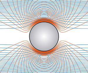
Figure 2 shows the radial variations of the dynamic perturbations to the tangential velocity, electrostatic potential and concentrations of the added  $\textrm {Na}^+$ and
  $\textrm {Cl}^-$ (the concentrations of
  $\textrm {DS}^-$ and its coion
  $\textrm {Na}^+$ are an order of magnitude smaller, so not shown) at
  $\omega / (2 {\rm \pi}) = 1$ MHz. Note that the electrolyte is the one in table 1 with a bulk surfactant concentration
  $c_\infty = 0.1$ mM (with
  $I_s = 1$ mM). To expedite a more rigorous test of the full model (blue lines), by comparison with the thin-double-layer model of Hill & Afuwape (Reference Hill and Afuwape2020) (red lines), the drop radius
  $a = 1\ \mathrm {\mu }\textrm {m}$, furnishing
  $\kappa a \approx 110$ with
  $\zeta e / (k_B T) = -7.08$. As expected, the velocity disturbances outside the diffuse layer (with scaled
  $r - \kappa a \gtrsim 1$) are in excellent agreement. Of course, the thin-double-layer model only captures the interfacial and electroosmotic slip, which manifest in the
  $E$-problem (on the right) when
  $r - \kappa a \sim 1$. Note also that the tangential velocity does not vanish as
  $r - \kappa a \rightarrow 0$, since the oil phase at the interface is mobile.

Figure 2. Tangential velocity (a, projection onto  $\boldsymbol {X} \in \{\boldsymbol {U}, \boldsymbol {E}\}$ for
  $\theta = {\rm \pi}/ 2$), electrostatic potential perturbation (b,
  $\theta = 0$) and added-salt ion-concentration perturbations (c,
  $\textrm {Cl}^-$ (blue) and
  $\textrm {Na}^+$ (red),
  $\theta = 0$) for the
  $U$- (left) and
  $E$- (right) problems:
  $\zeta e / (k_B T) = -7.08$,
  $a = 1\ \mathrm {\mu }\textrm {m}$,
  $\kappa ^{-1} = 9.18$ nm (
 $\kappa a \approx 110$),
  $\omega / (2 {\rm \pi}) = 10^6$ Hz. In (a and b), red lines are the theory of Hill & Afuwape (Reference Hill and Afuwape2020). Note that
  $u_\theta ^U$ and
  $u_\theta ^E$ are the velocity scaled with
  $U$ and the Smoluchowski-slip velocity, respectively.
  $\hat {\psi }^X$ and
  $\hat {n}^X_i$ are perturbations scaled according to Hill et al. (Reference Hill, Saville and Russel2003) with solid and dashed lines denoting the real and imaginary parts.
With respect to the fluctuating electrostatic potential, the numerical solution predicts  $O(10^{-4})$ (scaled) values within the diffuse layer for the
  $U$-problem, whereas the perturbation is zero according to the thin-double-layer model. For the
  $E$-problem, the numerical and approximate models agree only with respect to the imaginary part (dashed lines). This suggests that the real part of the electrostatic potential perturbation arises from diffusive charge transport that is not captured by the thin-double-layer model. Finally, note that ion-concentration perturbations oscillate with radial position, reaching large (scaled) electric-field-induced values within the diffuse layer. Again, the thin-double-layer approximation has zero ion-concentration perturbations (red and blue distinguish the two ions in these figures).
Figure 3 shows the same data as described above for figure 2, but with a drop radius  $a = 100$ nm giving
  $\kappa a \approx 11$. Although
  $\kappa a \gg 1$, the thin-double-layer model reveals that the real part of the electric-field-induced velocity disturbance now departs significantly from the numerical calculation. Clearly, the interfacial slip is much weaker, as is the electro-osmotic slip. Interestingly, the real part of the electric-field-induced electrostatic potential perturbation agrees with the thin-double-layer model. Under these conditions, the signs of the ion-concentration perturbations do not change within the diffuse layer.

Figure 3. The same as figure 2 but with  $a = 100$ nm (
 $\kappa a \approx 11$).
To examine in more detail the role of the drop radius on the dynamic mobility, figure 4 shows the magnitude and phase versus the scaled drop radius for three bulk surfactant concentrations  $c_\infty$, all with the same added-salt concentration
  $I_s = 1$ mM. Note that changing the surfactant concentration from
  $0.001$ to
  $8$ mM significantly changes the equilibrium surface charge and potential, whereas the Debye length is principally controlled by the fixed concentration of added salt. Other interfacial parameters are available in table 1. The figures compare the dynamic mobility at three frequencies spanning two decades. The numerical calculations (solid lines) are compared with the thin-double-layer theory for values of
  $\kappa a > 10$. Note that the lowest surface potential (
 $|\zeta | \approx 2.64 k_B T / e$) is large enough to ensure that the diffuse layer is predominantly occupied by counterions (
 $\textrm {Na}^+$), but not so large for the Smoluchowski-slip approximation to break down. Thus, the numerical calculations and thin-double-layer model are in excellent agreement at all three frequencies (spanning two decades). Further increasing the surface charge density generally places increasingly stringent demands on
  $\kappa a$ to maintain accuracy. Thus, based on these data, the thin-double-layer model demands
  $\kappa a \gtrsim 100$ when the surfactant concentration
  $c_\infty \gtrsim 0.1$ mM.

Figure 4. Dynamic electrophoretic mobility (magnitude and phase) spectra versus scaled drop radius: bulk added-salt concentrations  $I_s = 1$ mM, SDS concentrations
  $c_\infty = 0.001$ (a),
  $0.1$ (b) and
  $8$ (c) mM; frequencies
  $\omega / (2 {\rm \pi}) = 10^5$ (blue),
  $10^6$ (red) and
  $10^7$ (yellow) Hz. Solid lines: computations for fluid spheres. Dashed lines: theory of Hill & Afuwape (Reference Hill and Afuwape2020) (two-component electrolyte, high surface-charge density, high frequency, thin double layer). (a)
  $\zeta e/(k_BT) = -2.64$,
  $\kappa ^{-1} = 9.61\ \textrm {nm}$. (b)
  $\zeta e/(k_BT) = -7.08$,
  $\kappa ^{-1} = 9.18\ \textrm {nm}$. (c)
  $\zeta e/(k_BT) = -8.68$,
  $\kappa ^{-1} = 3.21\ \textrm {nm}$.
It is pertinent to briefly address the droplet mobility as reported by de Aguiar et al. (Reference de Aguiar, de Beer, Strader and Roke2010), as discussed in § 1. Recall, these experiments were conducted using an electrophoretic light-scattering apparatus for which the frequency of the electric field considered low enough to induce a quasi-steady dynamics. With negligible added salt, the isotherm of Hill & Afuwape (Reference Hill and Afuwape2020) furnishes the interfacial characteristics summarized in table 3. It is shown that the surface potential  $|\zeta |\gtrsim 8.5 k_B T / e \approx 213$ mV at SDS concentrations greater than
  $1$ mM. Based on the Smoluchowski mobility formula (rigid spheres with
  $\kappa a \gg 1$), we would expect dimensionless mobilities
  $|M^*| \gtrsim 13$, almost twice as large as registered by de Aguiar et al. (Reference de Aguiar, de Beer, Strader and Roke2010) when
  $c_s = 8$ mM.
Table 3. Isotherm calculations for SDS (below the critical micelle concentration) at the hexadecane–water interface: added-salt (NaCl) concentration  $I_s = 1\ \mathrm {\mu }\textrm {M}$, oil–water surface tension (without surfactant)
  $\gamma (0,0) = 47\ \textrm {mN}\,\textrm {m}^{-1}$. Bulk SDS concentration
  $c_\infty$, equilibrium
  $\textrm {DS}^-$ surface concentration
  $c^0$.

Mobilities predicted by the present model for fluid drops are plotted in figure 5. Note that these are calculated at a frequency  $\omega / (2 {\rm \pi}) = 0.01$ MHz, since the numerical solution breaks down at lower frequencies (the far-field fluid boundary conditions apply further and further from the interface as
  $\omega \rightarrow 0$). Nevertheless the small phase angle suggests that the dynamics is quasi-steady. Thus, to register the mobility
  $M^* \approx -7$ reported by de Aguiar et al. (Reference de Aguiar, de Beer, Strader and Roke2010), the drop radius
  $a \approx 790$ nm, as also predicted by the standard electrokinetic model for rigid spheres (O'Brien & White Reference O'Brien and White1978).

Figure 5. Dimensionless mobility magnitude  $|M^*|$ for SDS-stabilized hexadecane droplets (
 $\omega / (2 {\rm \pi}) = 10$ kHz for which
  $|\angle M^*| \lesssim 6^\circ$) versus drop radius
  $a$ for bulk surfactant concentrations
  $c_s = 8$ (blue),
  $1.0$ (red) and
  $0.01$ (yellow) mM (added salt concentration
  $I_s = 1\ \mathrm {\mu }\textrm {M}$). Horizontal lines are the mobilities reported (as Smoluchowski
  $\zeta$-potentials) in figure S1 of de Aguiar et al. (Reference de Aguiar, de Beer, Strader and Roke2010); these suggest (light-scattering, intensity weighted) drop radii
  ${\sim }800\text {--}2000$ nm, increasing with decreasing surfactant concentration.
Calculations with lower SDS concentrations suggest a radius and increases with decreasing SDS concentration, reaching  $a \gtrsim 2\ \mathrm {\mu }\textrm {m}$ when
  $c_s = 0.01$ mM. These are significantly larger than ascertained by the (number-weighted) radius (
 $83$ nm) that de Aguiar et al. (Reference de Aguiar, de Beer, Strader and Roke2010) reported from dynamic light scattering. Note that electrophoretic mobilities from light-scattering electrophoresis are averaged according to the light-scattering intensity (with units of kcps), thus weighted according to
  $a^6$ (Russel et al. Reference Russel, Saville and Showalter1989). Therefore, if the number-averaged distribution of de Aguiar et al. could be recalculated with a weighting proportional to
  $a^6$, then the resulting average may indeed be closer to the size inferred by the average mobility/
 $\zeta$-potential. Volume-weighted size should fall between number- and intensity-weighted values. For example, percentiles for a log-normal distribution (by volume) of SDS-stabilized hexadecane drops in water containing NaCl (
 $\phi = 0.05$,
  $c_s = 5$ mM,
  $I_s = 1$ mM) have been reported (from acoustic attenuation)
  $(d_{15}, d_{50}, d_{80}) = (170, 314, 580)$ nm (Djerdjev & Beattie Reference Djerdjev and Beattie2008). As expected, these fall between the foregoing number (
 $a \approx 83$ nm) and intensity (predicted
  $a \sim 790$ nm) averages for similar SDS-stabilized hexadecane emulsions.
Figure 6 shows the dynamic drag coefficient accompanying the dynamic mobilities in figure 4. As might be expected from the  $U$-problem perturbations in figure 3, the thin-double-layer model provides an excellent approximation of the dynamic drag, since this problem is dominated by hydrodynamics (viscous and temporal fluid inertia) with weak electro-viscous effects. It follows that acoustic-attenuation determinations of emulsion drop size, which hinge on hydrodynamic drag – among many other significant dissipative mechanisms in emulsions (Temkin Reference Temkin2005) – is less susceptible to Marangoni effects than the dynamic mobility (Hill & Afuwape Reference Hill and Afuwape2020).

Figure 6. The dynamic drag coefficient accompanying the mobilities in figure 4. (a)  $\zeta e/(k_BT) = -2.64$,
  $\kappa ^{-1} = 9.61\ \textrm {nm}$. (b)
  $\zeta e/(k_BT) = -7.08$,
  $\kappa ^{-1} = 9.18\ \textrm {nm}$. (c)
  $\zeta e/(k_BT) = -8.68$,
  $\kappa ^{-1} = 3.21\ \textrm {nm}$.
5. Discussion
Here, we examine the role of model parameters when they are outside the range above for SDS-stabilized hexadecane–water emulsions. Calculations for rigid spheres having the same interfacial characteristics as the drops in figures 4 and 6, but with  $\eta _i / \eta _o \gtrsim 10^2$, are available in appendix C. Baygents & Saville (Reference Baygents and Saville1991) showed that the zero-frequency mobility of spherical drops becomes independent of
  $\eta _i / \eta _o$ when
  $\kappa a \lesssim 1$, otherwise increasing with
  $\eta _i / \eta _o$. This also seems to be the case for the dynamic mobility. However, the differences are rather subtle for the hexadecane–water couple with
  $\eta _i / \eta _o \approx 3.9$, thus motivating the following more detailed examination of how the internal viscosity affects the dynamic mobility.
5.1. Internal viscosity contrast
Figure 7 shows how the dynamic mobility transits from the fluid- to rigid-sphere limits when varying the internal viscosity (scaled with  $\eta _o$) at
  $\omega / (2 {\rm \pi}) = 1$ and
  $10$ MHz, for drops with four radii spanning the range
  $a = 10\text {--}10^4$ nm. Note that the thin-double-layer model (dashed lines) is shown only for the two radii with
  $\kappa a > 100$. Increasing the drop viscosity suppresses the Marangoni effects, so only the mobilities with
  $\eta _i / \eta _o \rightarrow 0$ are expected to reflect Marangoni effects. Note also that the interfacial mobility of DS
 $^-$ has been allowed to vary with
  $\eta _i$. Here, this is accomplished – for illustrative purposes – by adopting an interfacial DS
 $^-$ friction coefficient (proportional to the reciprocal interfacial diffusivity) that is weighted so the effective viscosity is
  $0.1 \eta _o + 0.9 \eta _i$; thus, crudely assuming that 10 % of the chain-like molecule resides in the inner fluid, and that its partitioning/conformation is independent of the change in internal viscosity.

Figure 7. Dynamic mobility (magnitude and phase) versus the internal viscosity (scaled with the external viscosity):  $(a, \kappa a) = (10 , 1.1)$ (blue),
  $(100, 11)$ (red),
  $(10^3, 110)$ (yellow) and
  $(10^4, 1100)$ (violet) (nm, -). Here, the interfacial diffusivity of
  $\textrm {DS}^-$ varies as
  $D = D_1 / (0.1 + 0.9 \eta _i / \eta _o)$ with
  $D_1 = 3.9 \times 10^{-9}\ \textrm {m}^2\,\textrm {s}^{-1}$. Here,
  $\zeta e / (k_B T) = -7.08$,
  $I_s = 1$ mM,
  $c_\infty = 0.1$ mM (other parameters derived from the isotherm are available in table 1). Solid lines: computations for fluid spheres. Dashed lines: theory of Hill & Afuwape (Reference Hill and Afuwape2020) (
 $\kappa a \gg 1$) for
  $(a, \kappa a) = (10^3, 110)$ (yellow) and
  $(10^4, 1100)$ (violet) (nm, -). (a)
  $\omega /(2{\rm \pi} )=1\ \textrm {MHz}$. (b)
  $\omega /(2{\rm \pi} ) = 10\ \textrm {MHz}$.
When  $\kappa a \lesssim 1$ (blue lines in figure 7,
  $\kappa a \approx 1.1$), the mobility is independent of
  $\eta _i / \eta _o$, as expected from the zero-frequency mobilities of (Baygents & Saville Reference Baygents and Saville1991). Interestingly, the thin-double-layer model captures the mobility well at all viscosity ratios when
  $\kappa a$ is large enough. However, even for
  $\kappa a \approx 110$ (yellow lines in figure 7), it breaks down when the drop viscosity is very low (and the DS
 $^-$ mobility is high). Under these conditions, the mobility is especially sensitive to the frequency, taking a very large magnitude at
  $1$ MHz, and a very small magnitude (with large, negative phase angle) at
  $10$ MHz. Note that, with the prevailing
  $\kappa ^{-1} \approx 10$ nm, we find
  $\omega \kappa ^{-2} / D_1 \sim 1$ when
  $\omega / (2 {\rm \pi}) = 1$ MHz. As highlighted by
Hill & Afuwape (Reference Hill and Afuwape2020), the large- $\kappa a$ limit furnishes a mobility that increases with the internal viscosity (e.g. violet lines (
 $\kappa a \approx 1100$) in figures 7(a) and 7(b), and the yellow lines (
 $\kappa a \approx 110$) in figure 7(b)), as also revealed by the steady (zero frequency) electrophoretic mobility of drops with low, uniform surface charge (and therefore no Marangoni effects) (Booth Reference Booth1951). Thus, the increasing mobility magnitude with decreasing internal viscosity when
  $\eta _i / \eta _o \lesssim 1$ seems to be a dynamic effect, which is captured – only in a suggestive, qualitative manner – by the thin-double-layer model when
  $\kappa a$ is large, but not too large.
It is therefore not clear why the mobility magnitude increases (with decreasing  $\eta _i / \eta _o$ when
  $\eta _i / \eta _o \lesssim 1$) to such an extent that it exceeds the rigid-sphere value (e.g. solid yellow lines (
 $\kappa a \approx 110$) in figure 7a, and the solid red line (
 $\kappa a \approx 11$) in figure 7b). Also puzzling is that the mobility magnitude when
  $\kappa a \approx 110$ at
  $\omega / (2 {\rm \pi}) = 10$ MHz (yellow solid line in figure 7b) is very close to the thin-double-layer model, but the accompanying phase angle (which is not captured by the thin-double-layer model when
  $\eta _i / \eta _o \ll 1$) is so large (
 $< - 90^\circ$) that the effective drop charge (as deduced by the sign of
  $\textrm {Re}{(M^*)}$) changes sign.
5.2. Electrostatic and interfacial concentration polarization
The foregoing suggest a mode of electrical polarization that is not completely captured by the thin-double-layer model, even when  $\kappa a \gg 1$ and
  $\omega a^2 / D \gg 1$. To help identify this polarization, figure 8 shows the real and imaginary parts of the electrostatic polarizability (scalar measure of the net electrostatic dipole strength, elaborated upon below) that accompany the mobilities in figure 7 at
  $\omega / (2 {\rm \pi}) = 1$ MHz. A careful inspection reveals that the real part (solid lines) scales in a much more systematic and significant manner with
  $\kappa a$. When
  $\kappa a \approx 110$ and
  $\eta _i / \eta _o \ll 1$,
  $\textrm {Re}{(P^*)}$ becomes especially large and positive, which is characteristic of drops for which
  $\kappa a$ is much smaller (e.g. figure 8 with
  $\kappa a \approx 11$ (red) and
  $1.1$).

Figure 8. Dimensionless electrostatic polarizability versus the internal viscosity (scaled with the external viscosity):  $(a, \kappa a) \approx (10 , 1.1)$ (blue),
  $(100, 11)$ (red),
  $(10^3, 110)$ (yellow) and
  $(10^4, 1100)$ (violet) (nm, -) with
  $\omega / (2 {\rm \pi}) = 1$ MHz. Here, the interfacial tension
  $\gamma ^0 \approx 0$, but the results are practically the same as with
  $\gamma ^0 = 0.892 \times 47\ \textrm {mN}\,\textrm {m}^{-1}$. Similarly to figure 7, the interfacial diffusivity of
  $\textrm {DS}^-$ varies as
  $D = D_1 / (0.1 + 0.9 \eta _i / \eta _o)$ with
  $D_1 = 3.9 \times 10^{-9}\ \textrm {m}^2\,\textrm {s}^{-1}$.
  $\zeta e / (k_B T) = -7.08$,
  $I_s = 1$ mM,
  $c_\infty = 0.1$ mM (other parameters derived from the isotherm are available in table 1). Solid and dashed lines denote real and imaginary parts. For
  $(a, \kappa a) \approx (10\ \mbox {nm}, 1.1)$ (blue),
  $\textrm {Re}{(P^*)} \sim 6$ and is therefore outside the range shown.
To help identify the origin of the large positive polarization, consider the thin-double-layer model of Hill & Afuwape (Reference Hill and Afuwape2020), for which the dipole strength (dimensional  $\hat {d}^E_\psi$, defined by
  $\psi ' = r (- 1 + \hat {d}^E_\psi r^{-3}) \boldsymbol {E} \boldsymbol{\cdot} \boldsymbol {e}_r$ for
  $r > a$) is
 \begin{equation} \hat{d}^E_\psi a^{-3} = \dfrac{\textrm{i} \omega \epsilon_o \epsilon_0 - \textrm{i} \omega \epsilon_i \epsilon_0 + 2 \sigma_s / a - \sigma_\infty + \dfrac{2 (z e)^2 c^0 D \,\textrm{i} \omega a^2 / (2 D)}{a k_B T (\textrm{i} \omega a^2 / (2 D) - 1)}}{- 2\,\textrm{i} \omega \epsilon_o \epsilon_0 - \textrm{i} \omega \epsilon_i \epsilon_0 + 2 \sigma_s / a + 2 \sigma_\infty + \dfrac{2 (z e)^2 c^0 D \,\textrm{i} \omega a^2 / (2 D)}{a k_B T (\textrm{i} \omega a^2 / (2 D) - 1)}}, \end{equation}
where  $\sigma _s$ is the surface conductivity arising from the diffuse-layer charge (O'Brien Reference O'Brien1986), and the terms proportional to
  $(z e)^2 c^0 = z e \sigma ^0$ capture interfacial diffusion and electro-migration of the adsorbed charge (adding these furnishes an effective surface conductivity
  $\sigma '_s$). Note that the dimensionless
  $\hat {d}^E_\psi a^{-3} \equiv P^*$,
  $\hat {d}^E_\psi \kappa ^{3} \equiv D^*$, and dimensionless
  $\lambda ' = \sigma '_s / (\sigma _\infty a)$ (also termed the Dukhin number).
If we now focus on frequencies ( ${\sim }1$ MHz) and emulsions for which
  $\omega a^2 / D \gg 1$,
  $\omega \epsilon _i \epsilon _0 / \sigma _\infty \ll 1$,
  $\omega \epsilon _o \epsilon _0 a / \sigma '_s \ll 1$ and
  $\epsilon _i / \epsilon _o \ll 1$ (e.g.
  $\sigma _\infty / (\epsilon _o \epsilon _0) \sim 53$ MHz for an NaCl, SDS electrolyte with ionic strength
  $I = 4.6$ mM (Hill & Afuwape Reference Hill and Afuwape2020)), then
 \begin{equation} P^* \approx \frac{2 \lambda' - 1}{2 \lambda' + 2}\quad \mbox{with}\ \lambda' \approx \frac{\sigma_s + (z e)^2 c^0 D / (k_B T)}{\sigma_\infty a}. \end{equation}
Thus,  $P^* \rightarrow -1/2$ and
  $1$ for
  $\lambda ' \rightarrow 0$ and
  $\infty$, respectively; these correspond to limits in which the polarization is dominated by dielectric polarization (
 $\lambda ' \ll 1$, negative dipole) and tangential free-charge migration (
 $\lambda ' \gg 1$, positive dipole). Figure 9 shows isocontours of the electrostatic potential satisfying Laplace's equation inside and outside a sphere with three representative dipole strengths. Note that electrical current (in the external electrolyte) flows along the electric field lines, i.e. perpendicular to the isocontours. Thus, when
  $P^* = -1/2$, this current is directed around the drop. However, when
  $P^* > 0$, current is directed into and out of the interfacial region, thus requiring an interfacial space-charge perturbation.

Figure 9. Isocontours of the perturbed electrostatic potential  $\psi '$ satisfying Laplace's equation for three values of the dimensionless dipole strength. The applied field
  $\boldsymbol {E}$ is directed from left to right. Blue (red) at the interface denotes (schematically) an excess of negative (positive) interfacial charge. See figure 10 for (complex-valued) counterparts calculated from the full model. (a)
  $P^{\ast} = -1/2$, (b)
  $P^{\ast}=1$, (c)
  $P^{\ast}=2$.
As acknowledged by Hill & Afuwape (Reference Hill and Afuwape2020), Hunter (Reference Hunter2001, § 8.9.1) has pointed out that thin-double-layer approximations founded on the Smoluchowski-slip analysis should break down when the ‘back field’ from the tangential migration of charge in the diffuse layer is not small compared to the applied field. Hunter shows that the ratio of the back field to the applied field is  ${\sim }\lambda '$, so increasing the surface charge density (increasing
  $|\zeta |$) with
  $\kappa a \ll 1$ (thin double layer) places increasingly stringent demands on
  $\kappa a \gg 1$ to maintain
  $\lambda ' \ll 1$. A comparison of the full model with the thin-double-layer approximation of Hill & Afuwape (Reference Hill and Afuwape2020) will therefore identify how large
  $\kappa a$ must be at the high surface-charge densities expected for SDS-stabilized emulsion drops. According to thin-double-layer calculations summarized in table 2 for drops with
  $a = 325$ nm,
  $\lambda \gtrsim 1$ (based on the diffuse-layer conductivity according to O'Brien (Reference O'Brien1986)), so variations in the drop size
  $a$ and the adsorbed-charge (
 $\textrm {DS}^-$) mobility
  $D / (k_B T)$ are expected to significantly influence the sign and magnitude of the polarization.
Figure 10 shows isocontours of the perturbed electrostatic potential  $\psi '$ at
  $\omega / (2 {\rm \pi}) = 1$ MHz, as furnished by the full model, for values of
  $\kappa a$ spanning the range
  ${\approx }1\text {--}10^3$. This sequence highlights the significant influence that drop size has on the electrical polarization. The smallest particle, with the largest (positive) dipole strength (figure 10a), produces a field that drives current (perpendicular to the iso-potential contours) radially at the oil–water interface; this necessitates diffusion to satisfy a no-flux boundary condition. For the largest particle (figure 10d), the (negative) dielectric polarization of the drop enables the tangential current in the (very thin) diffuse layer to balance the radial current, without inducing a space-charge perturbation. With
  $\kappa a \sim 100$ (figure 10c), however, the electric-field perturbation is very weak (vanishing dipole strength), suggesting a balancing of the dielectric polarization with the dynamic space-charge polarization. The fluctuating space charge is not accounted for in the thin-double-layer model, and so this seems to explain the breakdown of the Smoluchowski electroosmotic-slip formula, for which the electrical body force in the diffuse layer arises from the induced electric field acting on the equilibrium space charge.

Figure 10. Isocontours of the perturbed electrostatic potential  $[\hat {\psi }^E(r) - r] \cos {\theta }$ (dimensionless) with the model parameters in figure 7(a) for
  $\eta _i / \eta _o \approx 3.93$ (hexadecane in water) at
  $\omega / (2 {\rm \pi}) = 1$ MHz. The applied field
  $\boldsymbol {E}$ is directed from left to right. Blue and red lines denote the real and imaginary parts. (a)
  $\kappa a \approx 1.09$,
  $P^*\approx 5.3-0.25\textrm {i}$. (b)
  $\kappa a\approx 10.9$,
  $P^{*}\approx 0.90-0.065\textrm {i}$. (c)
  $\kappa a \approx 109$,
  $P^*\approx -0.052 + 0.097\textrm {i}$. (d)
  $\kappa a\approx 1090$,
  $P^*\approx -0.44 + 0.014\textrm {i}$.
5.3. Profiles for high- and low-viscosity drops
Figures 11 and 12 (with figures 18 and 19 in appendix D) show profiles of the velocity, electrostatic potential, and ion-concentration perturbations (as described in the caption of figure 2), but now with vary large and small values of the internal viscosity, for values of  $\kappa a \approx 10^2$ and
  $10^3$. Note that the ion-concentration perturbations (bottom panels) are plotted with a linearly scaled ordinate. While obscuring oscillations in the far field (e.g. figure 2), this helps to identify the sign and phase of the ion-concentration perturbations, particularly within the diffuse layer, where the electric-field-induced perturbations are especially large.


Figure 12. The same as figure 11, but with  $\eta _i / \eta _o = 100$.
In figure 11, the electric-field-induced (right panels) ion-concentration perturbations inside the diffuse layer are large and negative. Moreover, there is a larger depletion of  $\textrm {Na}^+$ counterions (red lines), suggesting that the net charge perturbation in the diffuse layer is negative, and, therefore, that the interfacial charge perturbation is positive, thus necessitating a negative interfacial concentration perturbation. The positive sign of the accompanying electrostatic potential perturbation suggests that the net electrostatic polarization principally reflects the interfacial-charge distribution that comes from the negative interfacial concentration perturbation.
In figure 12, where the interfacial charge is now tightly coupled to the interface by virtue of a high internal viscosity ( $\eta _i / \eta _o = 100$), the ion-concentration perturbations are very weak, with a net charge that changes sign within the diffuse layer. While the imaginary part of the electrostatic potential perturbation is similar to the case above (figure 11), the real part has changed sign, taking a large negative value. Moreover, while the imaginary part of the electrostatic potential perturbation agrees with the thin-double-layer model, the real part has a significantly larger magnitude. Contrary to figure 11, the velocity perturbations are in good agreement with the thin-double-layer model, as expected from the comparable magnitude and phase of the mobility in figure 7 when
  $\eta _i / \eta _o = 100$.
5.4. Interfacial-charge mobility
Figure 18 (appendix D) shows the profiles for a larger drop,  $(a, \kappa a) \approx (10^4\ \mbox {nm}, 1100)$, with a fluid-behaving interface. Recall, we have already established that the mobility under these conditions is consistent with the thin-double-layer model, as the velocity and electrostatic potential perturbation profiles confirm. However, in contrast to figure 11 with
  $(a, \kappa a) \approx (10^3\ \mbox {nm}, 110)$, the electrostatic potential perturbation has a large, negatively signed real part. This suggests that the underlying interfacial concentration (charge) perturbation is positive (negative), as one might expect if an advection-dominated interfacial charge migration were hydrodynamically coupled to electro-osmotic flow in the diffuse layer. As expected, tightly coupling the interfacial charge to the interface by virtue of a very high internal viscosity (
 $\eta _i / \eta _o = 100$), as seen in figure 19 (appendix D), attenuates the ion-concentration perturbations in the diffuse layer, but has no significant impact on the large, negatively signed real part of the electrostatic potential perturbation. Thus, the interpretation of the profiles in figures 11 and 12 (also appendix D) points to the thin-double-layer model breaking down due to the interfacial charge perturbation being coupled to the diffuse-layer charge perturbation rather than to the diffuse-layer flow.
The data in figure 13 have no Marangoni effects, but the interfacial mobility has been set– again for illustrative purposes – to a very large (and physically unacceptable) value. This makes the interfacial Péclet number for  $\textrm {DS}^{-}$ vanishingly small. Comparing to figure 7(a), setting
  ${Ma}_c \ll 1$ and
  ${Pe} \ll 1$ significantly impacts the mobility, particularly when
  $\kappa a \gg 1$. Most noteworthy is that the mobility decreases with increasing
  $\eta _i / \eta _o$, and that, even for the largest values of
  $\kappa a$, there is no correspondence with the thin-double-layer model of (Hill & Afuwape Reference Hill and Afuwape2020). When
  $\kappa a \approx 110$ (yellow lines in figure 13), the mobility is dominated by its large, negative imaginary part (dashed lines in figure 13b), with an electrical polarization that is dominated by a positive real part
  $\textrm {Re}{(P^*)} \approx 1$ (figure 13c). This suggests that the polarization is dominated by the interfacial concentration/charge polarization. If this is rapid, as evidenced by
  $\textrm {Re}{(P^*)} \approx 1$ being largely in phase with the electric field, then it would induce an electric field in the diffuse layer that opposes the applied field. The resulting electroosmotic flow would therefore be in the same direction as the force on the interfacial charge, as suggested by the large negatively signed mobility under these conditions.

Figure 13. The same as figure 7(a), but with  $\gamma ^0 \approx 0$ (
 ${Ma}_c \approx 0$) and
  $D = 10^6 D_1 / (0.1 + 0.9 \eta _i / \eta _o)$ (
 ${Pe} \ll 1$). Under these conditions, the dynamic polarizability
  $P^* = D^* / (\kappa a)^3 \approx 1$ for
  $\kappa a \gg 1$; such strong (positive) polarization drives electroosmotic flow in the opposite direction to that of the applied electric field.
Figure 14 is the same as figure 13, but the interfacial mobility is set to make the interfacial Péclet number very large, so the interfacial charge is strongly coupled to the interfacial velocity (again without Marangoni effects). Now the mobility and polarization are closer to the base case (figures 7 and 8), with a notably smaller mobility when  $\kappa a \approx 110$ and
  $\eta _i / \eta _o \ll 1$ (yellow lines). Thus, while the interfacial mobility is hindered by its vanishingly small diffusion coefficient, the charge is now immobilized on a mobile/fluid interface. The weaker electrical polarization (
 $\textrm {Re}{(P^*)} < 0$) drives a weaker reverse-acting electroosmotic flow.

Figure 14. The same as figure 7(a), but with  $\gamma ^0 \approx 0$ (
 ${Ma}_c \approx 0$) and
  $D = 10^{-6} D_1 / (0.1 + 0.9 \eta _i / \eta _o)$ (
 ${Pe} \gg 1$).
5.5. Kinetic exchange
Lastly, figure 15 explores the role of the kinetic-exchange coefficients. Recall, all the previous calculations are with  $k_d = k_a = 0$, ensuring that there is no exchange of surfactant between the interface and electrolyte. Here, the mobility and polarizability are plotted versus the scaled desorption kinetic coefficient
  $k_d / \omega$ with
  $\omega / (2 {\rm \pi}) = 1$ MHz. Note that the adsorption kinetic coefficient
  $k_a$ has been set so that
  $k_d / (\kappa k_a) = 1.1$, whereas, as discussed in the theory section, this ratio is required by the adsorption isotherm for
  $\textrm {DS}^-$ to be very small. Here, the electrokinetic response is confirmed to transit from a kinetic-rate-limited regime to a diffusion-limited regime when
  $k_d / \omega \sim 1$. This transition is significant only for the smallest drops with
  $\kappa a \sim 1$, otherwise the diffusion-limited regime is maintained by the high frequency, i.e.
  $\omega a^2 / D_1 \gg 1$ (
 $D_1$ is the
  $\textrm {DS}^-$ diffusivity in the electrolyte) for all but the smallest drops.

Figure 15. Dynamic mobility ( $M^*$, magnitude and phase, and real and imaginary) and polarizability (
 $P^* = D^* / (\kappa a)^3$, real and imaginary) versus the scaled desorption kinetic coefficient
  $k_d / \omega$ with
  $k_d / (\kappa k_a) \approx 1.1$:
  $(a, \kappa a) \approx (10 , 1.1)$ (blue),
  $(100, 11)$ (red),
  $(10^3, 110)$ (yellow) and
  $(10^4, 1100)$ (violet) (nm, -) with
  $\omega / (2 {\rm \pi}) = 1$ MHz. Other parameters:
  $\eta _i / \eta _o = 3.5 / 0.89$,
  $D = 1.08 \times 10^{-10}$ m
 $^2$ s
 $^{-1}$,
  $\zeta e / (k_B T) = -7.08$,
  $I_s = 1$ mM,
  $c_\infty = 0.1$ mM (other parameters derived from the isotherm are available in table 1). Solid and dashed lines denote real and imaginary parts. Note the transition from kinetic- to diffusion-limited exchange kinetics; however,
  $k_a$ is set (for illustrative purposes only) to a value that is
  $6$ orders of magnitude smaller than prescribed by the adsorption isotherm.
6. Summary
A computational model has been developed for the electrokinetic response of spherical drops to oscillatory forcing, accounting for interfacial dynamics (Marangoni, electrical and hydrodynamic stresses, coupled to ion electro-migration, diffusion and advection in the weak-field limit). The focus was on the dynamic electrophoretic mobility spectrum, which provides a theoretical foundation for interpreting electrokinetic sonic amplitude experiments. However, the model also furnishes the electro-static polarizability as a theoretical foundation for dielectric relaxation spectroscopy.
The calculations undertaken in this study centred about the charged drops encountered in SDS-stabilized oil-in-water emulsions. While these have served as electro-sterically stabilized emulsion models for many decades, they are still not well understood (as discussed in § 1). Here, computations established practical limits on the parameters for which a recent thin-double-layer model was derived by Hill & Afuwape (Reference Hill and Afuwape2020).
Owing to the very high surface-charge density (and accompanying surface conductivity), unusually stringent conditions are imposed on  $\kappa a$, with the Smoluchowski-slip approximation requiring
  $\kappa a \gtrsim 10^2$; otherwise, numerical solutions of the model are necessary, since there is no analytical-approximate theory available for
  $\kappa a\lesssim 1$.
The model was used to explore the significant role of electrical polarization and how it is influenced by interfacial-charge mobility. Unifying the interfacial thermodynamics (via an adsorption isotherm) and electrokinetic dynamics, over a wide range of frequencies, provides a framework for probing emulsion drops that have more complex interfacial dynamics; for example, as arising from self-assembled (e.g. Pickering) layers (Ortiz et al. Reference Ortiz, Pochat-Bohatier, Cambedouzou, Bechelany and Miele2020) with interfacial visco-elasticity (Kim et al. Reference Kim, Choi, Zasadzinski and Squires2011).
The present study was limited to weak electric fields, so it may be pertinent to advance the model to account for finite electric-field strengths. The case for which  $\kappa a \gg 1$, but the Dukhin number is not small, might be handled using the so-called small Dukhin number approximation, which has been applied to the steady electrophoretic mobility of dielectric particles in the thin-double-layer limit (Schnitzer & Yariv Reference Schnitzer and Yariv2014). The more general case seems to require a computational approach to handle broken fore–aft symmetry, and, possibly, shape perturbations.
Applying the present model to interpret experimental data may benefit from specific attention to the droplet size distribution. Having prescribed the interfacial properties from an adsorption isotherm, the mobility magnitude and phase were demonstrated here to be a sensitive and complex (e.g. non-monotonic magnitude) function of the drop size. The (number-weighted) dynamic light-scattering size distribution of de Aguiar et al. (Reference de Aguiar, de Beer, Strader and Roke2010) indicates a large number density of small ( $a \approx 83$ nm) drops, much smaller than reported from acoustic attenuation (e.g.
  $a \approx 85\text {--}290$ nm, Djerdjev & Beattie (Reference Djerdjev and Beattie2008)) and intensity-averaged light scattering (e.g.
  $a \approx 276\text {--}576$ nm, Barchini & Saville (Reference Barchini and Saville1996)). Note that Barchini and Saville also performed centrifugal fractionation steps (on silicone–oil emulsions), thus narrowing the size distribution.
Note that the electrophoretic mobility from electrophoretic light scattering is weighted toward scattering from the largest drops. On the other hand, the dynamic mobility, as measured by electro-acoustic instrumentation, is weighted by particle volume. The recommendation here is to adopt consistent determinations of particle size and mobility from light scattering, i.e. interpret the intensity-averaged mobility with an accompanying intensity-average size.
The present model suggests that electro-sterically stabilized bubble mobilities may be unusually high due to a high interfacial charge mobility. However, these conclusions were drawn from a crude analysis in which the interfacial-charge mobility is dominated by the (low) viscosity of the dispersed phase. In practice, the mobility of the interfacial charge is expected to depend on the geometry and thermodynamic affinity of the adsorbing species at a specific interface. This highlights, once again, the importance of complementing electrokinetic measurements with a specific adsorption isotherm.
Finally, the present model provides a quantitative theoretical framework for studying kinetic exchange of the adsorbing charge. For strongly adsorbing surfactants, this dynamics seems to be so slow (under MHz forcing of an ESA experiment) that it can be neglected. This might not be the case for much smaller adsorbing ions, such as  $\textrm {OH}^-$, which are also known to charge oil–water interfaces (Marinova et al. Reference Marinova, Alargova, Denkov, Velev, Petsev, Ivanov and Borwankar1996). The present model may provide new opportunities for interpreting interfacial charging dynamics, perhaps in micro-fluidic as well as electrokinetic diagnostic settings.
Acknowledgements
This work was supported by an NSERC Discovery Grant and sabbatical leave from McGill University. The author gratefully acknowledges NSERC Engage and Imperial Oil University Research Awards with Dr S. Mercer (Imperial Oil Limited), and the Fields Institute for funding to present an early part of this work at their workshops on ion transport (2017, 2019).
Declaration of interests
The author reports no conflict of interest.
Appendix A. Numerical solution
The interfacial model has two unknown constants  $d_c$ and
  $c_1$, which, recall, measure the interfacial concentration perturbation and interfacial velocity. Moreover, the functions with superscript ‘0’ come from a numerical solution of the equilibrium problem, furnishing
  $\psi ^0(r)$ and
  $n^0_i(r)$ from the spherical nonlinear Poisson–Boltzmann problem. The ‘hatted’ functions come from solving
  $N$ ion conservation equations, the Poisson equation, one scalar momentum/vorticity equation and the auxiliary relationship (
 $g = h_{r,rr}$), thus furnishing
  $\hat {n}_i(r)$,
  $\hat {\psi }(r)$,
  $h_r(r)$ and
  $g(r)$. These complex-valued functions can vary on multiple, widely separated length scales, so the solution is very challenging. The method adopted here is the one developed by Hill et al. (Reference Hill, Saville and Russel2003) by which the first- and second-order partial derivatives are approximated using centred finite differences on a non-uniform grid that adapts to the curvatures of the
  $N + 3$ functions. Typically
  ${\sim } 10^4$ grid points are required on a domain that may extend
  ${\sim } 10^2 \kappa ^{-1}$ from the interface. Boundary conditions on the outer-boundary respect the far-field asymptotic form for each function. The solution is accomplished in an efficient manner by adopting a single mesh on which all the functions are solved. This enables the algebraic finite-difference relationships for each equation at each grid point to be solved as a block-diagonal system. To preserve the block-diagonal form, the next section details how to implement the interfacial relationships above as boundary conditions.
At the interface, a ‘ghost’ grid point with index  $i = -1$ is positioned at radial position
  $r = a - \delta$ (see figure 16), so the centred difference approximations of the first and second derivatives of a function
  $\phi (r)$ at
  $r = a$ are
 \begin{equation} \phi_r = \frac{\phi_1 - \phi_{-1}}{2 \delta}\quad \mbox{and}\quad \phi_{rr} = \frac{\phi_{-1} + \phi_{1} - 2 \phi_0}{\delta^2}. \end{equation}
The interfacial equations above then take the linear form
 \begin{equation} \boldsymbol{a}_{-1} \boldsymbol{\cdot} \boldsymbol{\phi}_{-1} + \boldsymbol{a}_{0} \boldsymbol{\cdot} \boldsymbol{\phi}_{0} + \boldsymbol{a}_{1} \boldsymbol{\cdot} \boldsymbol{\phi}_{1} + \boldsymbol{b}\boldsymbol{\cdot} \boldsymbol{x} = \boldsymbol{c}, \end{equation}
where  $\boldsymbol {x} = [d_c, c_1]^\textrm {T}$, and
  $\boldsymbol {\phi }_i = [\hat {n}_1,\ldots ., \hat {n}_N, \hat {\psi }, g, h]_i^T$. Here, the subscripts distinguish the grid points at the interface.

Figure 16. Finite-difference coupling the interfacial and bulk conservation relationships. (a) Finite-difference grid at the drop–electrolyte interface. The grid point with index  $i = 0$ resides at the interface. (b) Global block-diagonal system.
The vectors  $\boldsymbol {x}$ and
  $\boldsymbol {\phi }_{-1}$ (variables peripheral to the global block-diagonal system) can now be expressed in terms of
  $\boldsymbol {\phi }_{0}$ and
  $\boldsymbol {\phi }_{1}$ (variables in the global block-diagonal system) as
 \begin{equation} \boldsymbol{x} = \bar{\boldsymbol{c}} - \bar{\boldsymbol{a}}_0 \boldsymbol{\cdot} \boldsymbol{\phi}_{0} - \bar{\boldsymbol{a}}_1 \boldsymbol{\cdot} \boldsymbol{\phi}_{1}, \end{equation}
and
 \begin{equation} \boldsymbol{\phi}_{-1} = \hat{\boldsymbol{c}} - \hat{\boldsymbol{a}}_0 \boldsymbol{\cdot} \boldsymbol{\phi}_{0} - \hat{\boldsymbol{a}}_1 \boldsymbol{\cdot} \boldsymbol{\phi}_{1}, \end{equation}
where
 \begin{equation} [\boldsymbol{x}, \boldsymbol{\phi}_{-1}]^\textrm{T} = [\boldsymbol{b}, \boldsymbol{a}_{-1} ]^{-1} \boldsymbol{\cdot} [\boldsymbol{c} - \boldsymbol{a}_{0} \boldsymbol{\cdot} \boldsymbol{\phi}_{0} - \boldsymbol{a}_{1} \boldsymbol{\cdot} \boldsymbol{\phi}_{1}]. \end{equation}
Next, with  $\boldsymbol {\phi }_{-1}$ expressed in terms of
  $\boldsymbol {\phi }_{0}$ and
  $\boldsymbol {\phi }_{1}$, the global system of equations for the grid point at the interface (index
  $i = 0$),
 \begin{equation} \boldsymbol{A}_{-1} \boldsymbol{\phi}_{-1} + \boldsymbol{A}_{0} \boldsymbol{\phi}_{0} + \boldsymbol{A}_{1} \boldsymbol{\phi}_{1} = \boldsymbol{B}_0, \end{equation}
is transformed to
 \begin{equation} \hat{\boldsymbol{A}}_{0} \boldsymbol{\cdot} \boldsymbol{\phi}_{0} + \hat{\boldsymbol{A}}_{1} \boldsymbol{\cdot} \boldsymbol{\phi}_{1} = \hat{\boldsymbol{B}}_0, \end{equation}
where
 \begin{equation} \hat{\boldsymbol{A}}_0 = \boldsymbol{A}_{0} - \boldsymbol{A}_{-1} \boldsymbol{\cdot} \hat{\boldsymbol{a}}_0, \quad \hat{\boldsymbol{A}}_1 = \boldsymbol{A}_{1} - \boldsymbol{A}_{-1} \boldsymbol{\cdot} \hat{\boldsymbol{a}}_1, \quad \hat{\boldsymbol{B}}_0 = \boldsymbol{B}_0 - \boldsymbol{A}_{-1} \boldsymbol{\cdot} \hat{\boldsymbol{c}}. \end{equation}
A conceptually similar approach is adopted for the outer (far-field) boundary, but the boundary conditions are sufficiently simple so as to avoid a formal matrix methodology. The global system reduces to a block-diagonal square matrix with global vector of unknowns  $[\boldsymbol {\phi }_0; \boldsymbol {\phi }_1; \ldots ]$.
To implement the foregoing methodology, the following details must be addresses, since the full matrix  $[\boldsymbol {b}, \boldsymbol {a}_{-1}]$ turns out to be singular. Firstly, the independent variable
  $g = h_{r,rr}$ is expressed as the finite-difference second derivative of
  $h_r$:
 \begin{equation} g_0 = \frac{h_{r,-1} + h_{r,1} - 2 h_{r,0}}{\delta^2}, \end{equation}
thus eliminating  $g$ from the interfacial system (it appears only in the interfacial momentum balance). Next, dropping the zero radial velocity condition furnishes a square
  $(N +4) \times (N+4)$ non-singular matrix
  $[\boldsymbol {b}, \boldsymbol {a}_{-1}]$ with
  $\boldsymbol {x} = [d_c, c_1]^\textrm {T}$ and
  $\boldsymbol {\phi }_i = [\hat {n}_1,\ldots , \hat {n}_N, \hat {\psi }, h_r ]^T_i$ (
 $i = -1, 0, 1$). The matrix inversion then provides
  $\boldsymbol {x}$ and
  $\boldsymbol {\phi }_{-1}$, from which (A 9) can be used to eliminate
  $h_{r,-1}$, thus enabling
  $g_0$ to be expressed in terms of all the other variables in
  $\boldsymbol {\phi }_0$ and
  $\boldsymbol {\phi }_1$:
 \begin{equation} g_0 \delta^2 + \sum_{j=1}^{N+2} \hat{a}_0(k,j) \phi_0(j) + \sum_{j=1}^{N+2} \hat{a}_1(k,j) \phi_1(j) - h_{r,1} + 2 h_{r,0} = \hat{c}(k). \end{equation}
Here, the index  $k$ identifies the row of the ‘hatted’ matrices furnishing
  $h_{r,-1}$. With (A 10), there are
  $N + 3$ independent relationships with which to eliminate the peripheral
  $\boldsymbol {A}_{-1}$ from the global system (see figure 16). Note that
  $\boldsymbol {a}_i$ are
  $(N+4) \times (N+2)$ matrices,
  $\hat {\boldsymbol {a}}_i$ are
  $(N+2) \times (N+2)$ and
  $\bar {\boldsymbol {a}}_i$ are
  $2 \times (N+2)$. Moreover,
  $\boldsymbol {c}$ is an
  $(N+4) \times 1$ vector,
  $\hat {\boldsymbol {c}}$ is
  $(N+2) \times 1$, and
  $\bar {\boldsymbol {c}}$ is
  $2 \times 1$. The momentum equation in the global system is coupled to
  $g_{-1}$, which is not provided by the foregoing interfacial model and matrix inversion. Nevertheless, this is remedied by simply replacing the momentum equation in the global system (for the grid point at the interface with
  $i = 0$) with the previously discarded zero radial velocity condition. With this prescription, the electrokinetic model faithfully reproduced computations for rigid spheres, and, as will be demonstrated below, provided accurate numerical validations of the analytical model of Hill & Afuwape (Reference Hill and Afuwape2020) for highly charged drops with Marangoni effects when
  $\kappa a \gg 1$.
The matrix inversion was accomplished using Gauss–Jordon operations with full pivoting (Press et al. Reference Press, Teukolsky, Vetterling and Flannery1988), adapted for complex arithmetic. Note that computing  $[\boldsymbol {b}, \boldsymbol {a}_{-1}]^{-1}$ and then performing matrix multiplications proved to be inaccurate (e.g.
  $[\boldsymbol {b}, \boldsymbol {a}_{-1}]^{-1} \boldsymbol {\cdot } [\boldsymbol {b}, \boldsymbol {a}_{-1}] \ne \boldsymbol {I}$). Accordingly, the inversion and subsequent matrix–vector multiplications were accomplished by simultaneously row reducing an augmented matrix of ‘right-hand’ vectors (e.g.
  $[\boldsymbol {c}, \boldsymbol {a}_0, \boldsymbol {a}_1]$) accompanying the row and column operations to invert
  $[\boldsymbol {b}, \boldsymbol {a}_{-1}]$.
Appendix B. Non-dimensionalization
The numerical solution is undertaken with variables scaled according to Hill et al. (Reference Hill, Saville and Russel2003), summarized as follows. Characteristic scales (subscript ‘ $c$’) for time, radial position, electrostatic potential, electric field, velocity, ion bulk concentration, and ion surface concentration are, respectively
 \begin{equation} \left.\begin{array}{c@{}} t_c = \omega^{-1}, \quad r_c = \kappa^{-1}, \quad \psi_c = k_B T / e, \quad E_c = \kappa k_B T / e \\ u_c = \epsilon_o \epsilon_0 (k_B T / e)^2 / (\eta_o a), \quad n_c = 2 I, \quad c_c = 2 I \kappa^{-1}. \end{array}\right\} \end{equation}
It follows that the dimensional groups  $[\cdot ]$ used to scale each variable/function
  $(\cdot )$ are
 \begin{equation} [\hat{n}^X_i] = 2 I / X, \quad [\hat{\psi}^X] = k_B T / (e X) , \quad [\,f^X] = [h_r^X] = u_c \kappa^{-1} / X, \quad [g^X]= u_c \kappa / X, \end{equation}
and
 \begin{equation} [d^X_c] = 2 I \kappa^{-1} / X, \quad [c^X_1] = \kappa u_c / X. \end{equation}
Note that we also have (dimensional  $\psi ^0_r$,
  $\sigma ^0$,
  $c^0$)
 \begin{equation} \psi^0_r = - \frac{\sigma^0}{\kappa \epsilon_o \epsilon_0 k_B T / e}, \quad \sigma^0 = z e c^0, \end{equation}
so (dimensionless  $\psi ^0_r$,
  $c^0$)
 \begin{equation} \psi^0_r = - \frac{z c^0 2 I e^2}{\kappa^2 \epsilon_o \epsilon_0 k_B T} = -z c^0. \end{equation}
For example, in dimensionless variables, the electrostatic potential is
 \begin{align} \psi(\boldsymbol{x},t) = \psi^0(r) + [\hat{\psi}^E(r) - M \hat{\psi}^U(r) - r] \,\textrm{e}^{-\textrm{i} t}\boldsymbol{E} \boldsymbol{\cdot} \boldsymbol{e}_r \rightarrow D^* r^{-2} \boldsymbol{E} \boldsymbol{\cdot} \boldsymbol{e}_r\quad \mbox{as}\ r \rightarrow \infty, \end{align}
and the ion-concentration perturbations are
 \begin{equation} n_i(\boldsymbol{x},t) = n_i^0(r) + [\hat{n}_i^E(r) - M \hat{n}_i^U(r)]\,\textrm{e}^{-\textrm{i} t} \boldsymbol{E} \boldsymbol{\cdot} \boldsymbol{e}_r \rightarrow 0\quad \mbox{as}\ r \rightarrow \infty. \end{equation}
Now the scaled/dimensionless interface and boundary conditions (compatible with the MPEK software package (Hill et al. Reference Hill, Saville and Russel2003) solution of the standard electrokinetic model) can be written as follows:
(i) Zero radial velocity
(B 8)\begin{equation} h_r = \kappa a U / (2 X). \end{equation}(ii) Interfacial (tangential) momentum conservation
(B 9)where\begin{equation} - \frac{\eta_i }{\eta_o}T_i(\varOmega_i a^2) c_1 - g = {Ma}\, d_c + (\hat{\psi} - \kappa a E / X) c^0 z, \end{equation}${Ma} = \gamma ^0 \beta / (k_B T) = {Ma}_c \eta _o D / (k_B T c^0 a)$ with concentration Marangoni number ${Ma}_c = \gamma ^0 \beta c^0 a / (\eta _o D)$ (Hill & Afuwape Reference Hill and Afuwape2020). Note that ${Ma} \sim 1$ is a dimensionless number of intrinsic interfacial properties (comparing interfacial and thermal energy), whereas the concentration Marangoni number ${Ma}_c \gtrsim 1$ compares interfacial diffusion and surface-tension relaxation times.(iii) Continuous tangential velocity
(B 10)\begin{equation} h_{rr} = U / (2 X) - c_1 \kappa a V_i(\varOmega_i a^2). \end{equation}(iv) Interfacial Gauss condition
(B 11)\begin{equation} \frac{\epsilon _i }{\epsilon_o} (\hat{\psi} / (\kappa a) - E / X) - (\hat{\psi}_r - E / X) = z d_c. \end{equation}(v) Interfacial species conservation (for the adsorbing species,
$i = 1$)
(B 12)where the interfacial Péclet number\begin{equation} \left( \frac{\textrm{i} \omega a^2}{2 D} - 1 - \frac{k_d a^2}{2D} \right) d_c + \frac{ k_a \kappa a^2}{2 D} \hat{n}_1 - (\hat{\psi} - \kappa a E / X) c^0 z = - c^0 \kappa a \,{Pe} \,V_i(\varOmega_i a^2) c_1, \end{equation}${Pe} = u_c a / D$.(vi)
$N$ radial ion fluxes
(B 13)\begin{equation} \left.\begin{array}{cc@{}} 0 = \hat{n}_{i,r} + \psi^0_r z_i \hat{n}_i + (\hat{\psi}_r - E/X) z_i n_i^0, & i=1 \\ - \dfrac{k_d}{D_i \kappa^2} d_c + \dfrac{k_a}{D_i \kappa} \hat{n}_i = \hat{n}_{i,r} + \psi^0_r z_i \hat{n}_i + (\hat{\psi}_r - E/X) z_i n_i^0, & i = 2,\ldots, N. \end{array}\right\} \end{equation}


With finite-difference approximations of the radial derivatives, these furnish (for demonstrative simplicity with  $N = 1$)
 \begin{equation} \boldsymbol{a}_{-1} \boldsymbol{\cdot} \boldsymbol{\phi}_{-1} = \left(\begin{matrix} 0 & 0 & 0 \\ 0 & 0 & 1 / (\delta^2)\\ 0 & 0 & -1 / (2 \delta)\\ 0 & 1 / (2 \delta) & 0 \\ -1 / (2 \delta) & -z_i n_i^0 / (2 \delta) & 0 \end{matrix}\right) \left(\begin{matrix} \hat{n}_{i,-1} \\ \hat{\psi}_{-1} \\ h_{r,-1} \end{matrix}\right), \end{equation}
 \begin{equation} \boldsymbol{a}_{0} \boldsymbol{\cdot} \boldsymbol{\phi}_{0} = \left(\begin{matrix} k_a \kappa a^2 / (2 D) & - c^0 z & 0\\ 0 & c^0 z & -2 / \delta^2 \\ 0 & 0 & 0 \\ 0 & (\epsilon_i / \epsilon_o) / (\kappa a) & 0\\ \psi_r^0 z_i - k_a /(D_i \kappa) & 0 & 0 \end{matrix}\right) \left(\begin{matrix} \hat{n}_{i,0} \\ \hat{\psi}_0 \\ h_{r,0} \end{matrix}\right), \end{equation}
 \begin{equation} \boldsymbol{a}_{1} \boldsymbol{\cdot} \boldsymbol{\phi}_{1} = \left( \begin{matrix} 0 & 0 & 0\\ 0 & 0 & 1 / \delta^2\\ 0 & 0 & 1 / (2 \delta)\\ 0 & -1 / (2 \delta) & 0\\ 1 / (2 \delta) & z_i n_i^0 /(2 \delta) & 0 \end{matrix} \right) \left( \begin{matrix} \hat{n}_{i,1} \\ \hat{\psi}_1 \\ h_{r,1} \end{matrix}\right), \end{equation}
 \begin{equation} \boldsymbol{b} \boldsymbol{\cdot} \boldsymbol{x} = \left( \begin{matrix} \textrm{i} \omega a^2 / (2 D) - 1 - k_d a^2 / (2D) & c^0 \kappa a \,{Pe} \,V_i(\varOmega_i a^2) \\ {Ma} & (\eta_i / \eta_o) T_i(\varOmega_i a^2) \\ 0 & \kappa a V_i(\varOmega_i a^2) \\ -z & 0 \\ k_d / (D_i \kappa^2) & 0 \end{matrix}\right) \left(\begin{matrix} d_c \\ c_1 \end{matrix}\right), \end{equation}
 \begin{equation} \boldsymbol{c} = \left(\begin{matrix} - \kappa a c^0 z E/X\\ \kappa a c^0 z E / X \\ U/(2X) \\ ( \epsilon_i / \epsilon_o - 1) E / X \\ z_i n_i^0 E / X \end{matrix} \right), \end{equation}
where the rows are ordered (top to bottom): interfacial species conservation, interfacial (tangential) momentum conservation, continuous tangential velocity, interfacial Gauss condition and interfacial species conservation (for the adsorbing species,  $i = 1$).
Appendix C. Rigid-sphere calculations

Figure 17. The same as figure 4 in the main text, but for rigid drops (achieved by setting  $\eta _i / \eta _o \gtrsim 10^2$ with
  $D \approx 10^{-12}\ \textrm {m}^2\,\textrm {s}^{-1}$). (a)
  $\zeta e/(k_BT) = -2.64$,
  $\kappa ^{-1} = 9.61\ \textrm {nm}$. (b)
  $\zeta e/(k_BT) =-7.08$,
  $\kappa ^{-1} = 9.18\ \textrm {nm}$. (c)
  $\zeta e/(k_BT) = -8.68$,
  $\kappa ^{-1} = 3.21\ \textrm {nm}$.
Appendix D. Profiles for large drops

Figure 18. The same as figure 11 in the main text (low-viscosity drop without Marangoni effects), but with larger  $(a, \kappa a) \approx (10^4\ \mbox {nm}, 1100)$.

Figure 19. The same as figure 11 in the main text (low-viscosity drop without Marangoni effects), but with larger  $(a, \kappa a) \approx (10^4\ \mbox {nm}, 1100)$ and
  $\eta _i / \eta _o = 100$.


