


1. Introduction
Particle dynamics plays a central role in living and non-living confined colloidal suspensions, with broad impact on biological engineering, the industrial and agricultural industries and pharmaceuticals. For example, diffusive transport of biomolecules plays a central role in life-essential processes in biological cells (Maheshwari et al. Reference Maheshwari, Sunol, Gonzalez, Endy and Zia2019). One recently demonstrated example is protein synthesis in Escherichia coli (E. coli), where changes in the relative abundances of biomolecules of different sizes drives changes in packing fraction and diffusivity of the biomolecules that, in consequence, play a key role in the transport latency associated with protein synthesis rates (Maheshwari et al. Reference Maheshwari, Gonzalez, Sunol, Endy and Zia2021). Confined dynamics plays an important role in the functionality of many industrial suspensions as well, for example the application and curing of particle-laden droplets such as pesticides, coatings and paints, which is a complex function of particle concentration, size polydispersity and confinement (Galliker et al. Reference Galliker, Schneider, Eghlidi, Kress, Sandoghdar and Poulikakos2012; Gilet & Bourouiba Reference Gilet and Bourouiba2014; Bansal, Basu & Chakraborty Reference Bansal, Basu and Chakraborty2017). In the pharmaceutical industry and research, some drug delivery mechanisms rely on enclosing a therapeutic suspension within vesicles, where stability inside the vesicle can be affected by polydispersity (Grenha et al. Reference Grenha, Remu nán-López, Carvalho and Seijo2008; Wilhelm et al. Reference Wilhelm, Lavialle, Péchoux, Tatischeff and Gazeau2008). The impact of size polydispersity on the colloidal dynamics has been studied to some extent in unconfined suspensions, providing a baseline for understanding these effects in confined systems.
For unconfined suspensions it is well known that the presence of size polydispersity modifies suspension structure and dynamics and can fundamentally change phase and flow behaviour. For example, size polydispersity changes the maximum packing fraction well beyond that of a monodisperse suspension, which is widely used in industry as a strategy to prevent cracking during drying, to reduce the number of coating steps or to repair antiquities without generating drying stress (Santiso & M’uller Reference Santiso and M’uller2002; Miltiadou-Fezans et al. Reference Miltiadou-Fezans, Kalagri, Kakkinou, Ziagou, Delinikolas, Zarogianni and Chorafa2008; Farr & Groot Reference Farr and Groot2009). Polydispersity can also alter phase behaviour, for example by delaying crystallization or suppressing it altogether, leading to vitrification (Pusey & van Megen Reference Pusey and van Megen1986; Van Megen & Underwood Reference Van Megen and Underwood1994; Brambilla et al. Reference Brambilla, El Masri, Pierno, Berthier, Cipelletti, Petekidis and Schofield2009; Zaccarelli, Liddle & Poon Reference Zaccarelli, Liddle and Poon2015) – a problem that has plagued the industrial coatings industry for decades but also was recently shown to underlie survival strategies in bacteria (Parry et al. Reference Parry, Surovtsev, Cabeen, O'Hern, Dufresne and Jacobs-Wagner2014). Polydispersity also modifies the flow rheology of a suspension, for example by imparting a qualitative and sometimes dramatic influence on viscosity (Chong, Christiansen & Baer Reference Chong, Christiansen and Baer1971; Poslinski et al. Reference Poslinski, Ryan, Gupta, Seshadri and Frechette1988; Rodriguez, Kaler & Wolfe Reference Rodriguez, Kaler and Wolfe1992), and can lead to the formation of channels (Allen & Uhlherr Reference Allen and Uhlherr1989; Daugan et al. Reference Daugan, Talini, Herzhaft, Peysson and Allain2004) or margination (Semwogerere & Weeks Reference Semwogerere and Weeks2008; Qi & Shaqfeh Reference Qi and Shaqfeh2018). Entropic and hydrodynamic effects underlie these rich behaviours: size intermixing reduces free energy to permit higher packing fractions; non-continuum colloidal interactions lead to vitrification rather than crystallization; and hydrodynamic asymmetry effects and depletion forces lead to margination and viscosity changes. Given the recently demonstrated interplay between spherical confinement and these microscopic forces (Aponte-Rivera, Su & Zia Reference Aponte-Rivera, Su and Zia2018), it is likely that new behaviours resulting from a coupling between confinement and polydispersity will affect the particle dynamics. The study of particle dynamics in confinement presents some of the same challenges as in the study of particle dynamics in unconfined suspensions, and presents new challenges as well.
The current experimental exploration of colloidal dynamics inside biological cells and particle-laden droplets contends with the competing demands of spatial and temporal resolution, which sometimes forces a tradeoff. Single-particle tracking techniques (Mattheyses, Simon & Rappoport Reference Mattheyses, Simon and Rappoport2010; Xiao et al. Reference Xiao, Wei, Cheng, He and Yeung2011; Sun et al. Reference Sun, Gu, Wang and Fang2012; Willets et al. Reference Willets, Wilson, Sundaresan and Joshi2017; Kim et al. Reference Kim, Nam, Lim and Suh2019; Kovari et al. Reference Kovari, Dunlap, Weeks and Finzi2019) aim to provide the sizes and dynamics of target colloidal objects. However, current experimental techniques for the study of highly mobile, dense and polydisperse suspensions face two primary challenges: the need for a uniform background and high frame-rate to particle-velocity ratio (Chenouard et al. Reference Chenouard2014; Ma et al. Reference Ma, Wang, Liu, Wei and Xiao2019). These challenges become more pronounced for confined systems, where capturing images of the interactions with the confining boundary requires high contrast (difference in refractive index) between the suspended particles and the wall (Ma et al. Reference Ma, Wang, Liu, Wei and Xiao2019). Such complications can in principle be avoided via numerical modelling, where positions and velocities of particles ranging from nanometres to microns can be monitored over macroscopic distances, and with fine temporal resolution over intervals much longer than those of microscopic transport or reaction processes. However, faithful numerical modelling of microscopic physics of colloidal hydrodynamics requires accurate modelling of Brownian motion, many-body hydrodynamic interactions, confinement and crowding. Most prior models neglect one or more of these effects, which can be appropriate approximations in some contexts (Ando & Skolnick Reference Ando and Skolnick2010; McGuffee & Elcock Reference McGuffee and Elcock2010; Chow & Skolnick Reference Chow and Skolnick2015; Li et al. Reference Li, Jiang, Singh, Heinonen, Hernández-Ortiz and de Pablo2020), but the problem being studied here requires all three. Our confined Stokesian dynamics algorithm models Brownian motion, many-body hydrodynamic interactions, confinement and crowding, but thus far could not represent polydisperse particle size (Aponte-Rivera & Zia Reference Aponte-Rivera and Zia2016; Aponte-Rivera et al. Reference Aponte-Rivera, Su and Zia2018). Size polydispersity is a non-trivial extension of both the hydrodynamics theoretical framework and the computational algorithm.
It is the objective of this work to study the impact of confinement and size polydispersity on the dynamics of confined colloidal suspensions by expanding our confined Stokesian dynamics framework. Our model expands the fundamental Stokesian dynamics algorithm developed by Brady and co-workers (Durlofsky, Brady & Bossis Reference Durlofsky, Brady and Bossis1987; Bossis & Brady Reference Bossis and Brady1989; Sierou & Brady Reference Sierou and Brady2001; Banchio & Brady Reference Banchio and Brady2003), which provides high accuracy and efficiency by effectively bypassing the details of fluid motion and focusing computational power on particle motion. Fluid motion and its effect on particle motion are incorporated by combining Ladyzhenskaya's integral expression (Ladyzhenskaya Reference Ladyzhenskaya1963) for fluid velocity with Faxén formulae (Faxén Reference Faxén1922) to give particle motion. A key element in this framework is the separation of hydrodynamic couplings into far-field many-body interactions, accomplished by developing analytical couplings known as resistance and mobility tensors, with near-field lubrication theory and pair-hydrodynamics functions (Jeffrey & Onishi Reference Jeffrey and Onishi1984; Jeffrey Reference Jeffrey1992; Jones Reference Jones2009). In our previous work we constructed an entirely new version of this framework for confinement (Aponte-Rivera & Zia Reference Aponte-Rivera and Zia2016; Aponte-Rivera et al. Reference Aponte-Rivera, Su and Zia2018). However, none of the many-body couplings were explicitly worked out for polydisperse particle size. Here, we expand our computational algorithm to model different particle sizes, for any degree of size polydispersity. To do so, we incorporated explicitly the difference in size in both the multipole expansion that describes disturbance flows generated by the particles, and in the Faxén laws that relate those flows to particle motion, all with finite confinement. Our prior work leveraged a crucial simplification of mobility matrices based on symmetry relations that are valid only for same-size particles; this symmetry is lost for polydisperse size. While the symmetry of the total grand mobility tensor remains, each diagonal and off-diagonal entry requires different algebraic expressions reflecting the different particle sizes that are coupled hydrodynamically. We carried out the same careful accounting of different particles sizes for the lubrication interactions between interacting pairs – particle–particle and particle–cavity, generating a model that rigorously accounts for many-body hydrodynamic and lubrication interactions in a confined colloidal dispersion of arbitrary particle-size distribution, cavity size and volume fraction (from dilute to maximum packing). Here, we employ the model to study the dynamics of confined, polydisperse suspensions, for a wide range of concentrations, particle-size ratios and particle-to-cavity size ratios, as well as various volume compositions, focusing on a bidisperse suspension to establish the basic interplay between confinement, hydrodynamics, entropic forces and particle-size differences on structure and dynamics.
The rest of this paper is organized as follows. In § 2, we describe the theoretical aspects of the polydisperse confined Stokesian dynamics framework as well as the methods utilized to calculate the short- and long-time self-dynamics of the confined particles. An in-depth analysis of the changes induced in the structure and particle dynamics by coupling polydispersity and confinement is given in § 3. Finally, § 4 offers conclusions and a discussion of the broader impact of our results on the understanding of biological and non-living confined suspensions.
2. Methods
The confined Stokesian dynamics algorithm developed by Zia and coworkers (Aponte-Rivera & Zia Reference Aponte-Rivera and Zia2016; Aponte-Rivera et al. Reference Aponte-Rivera, Su and Zia2018) is expanded in this work to describe the dynamics of unequal-sized hard spheres confined by a spherical cavity. A brief outline of the methods follows.
2.1. Model system
We consider a system of  $N$ hard spheres of different hydrodynamic sizes suspended in a Newtonian fluid of constant viscosity
  $\eta$ and density
  $\rho$, all confined inside a hard spherical cavity of radius
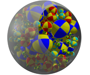
  $R$ (figure 1a). The suspended spheres are of
  $K$ different sizes
  $a_K> a_{K-1} > \ldots > a_i > \ldots > a_1$, with
  $N_i$ particles each of radius
  $a_i$, and
  $N = \sum _i^{K} N_i$. The size of one species of colloids relative to another is
  $\lambda _{p(i)}$ and is set without loss of generality with respect to the radius of the smallest colloid, such that the particle-to-particle size ratio is always greater than unity,
  $\lambda _{p(i)}\equiv a_i/a_1>1$. The total volume fraction of particles
  $\phi$ is a simple sum over the volume fractions of the different size populations,
  $\phi = \sum _i^{K} \phi _i$, where
  $\phi _i = 4/3 {\rm \pi}a_i^{3}n_i$, and
  $n_i$ is the number density of particles with radius
  $a_i$ inside of the cavity. The degree of confinement is set by the ratio of the radius of a particle to the radius of the enclosing cavity,
  $\lambda _{c(i)}\equiv a_i/R<1$. Together, a set of
  $K$ values from
  $\lambda _{c(i)}\cup \lambda _{p(i)}$, and a set of
  $K$ values from
  $\phi _i\cup \phi$ fully specify the suspension composition of the model system.

Figure 1. (a) Conceptual sketch of model system for a spherically confined bidisperse ( $K=2$) suspension with (b) particle labelling based on size.
2.2. Modelling particle displacements in dense spherically confined colloidal suspensions
Modelling the motion of the suspended particles enables the computation of transport properties, and reveals how confinement, crowding and size polydispersity affect the particle dynamics and suspension rheology. All of the particles are colloidal and therefore their dynamics is described by the N-body Langevin equation
 \begin{equation} \boldsymbol{m}\boldsymbol{\cdot}\frac{\textrm{d}{\boldsymbol{U}}}{\textrm{d}t}= \boldsymbol{{F}}^{P} + \boldsymbol{{F}}^{{{Ext}}} + \boldsymbol{{F}}^{B} + \boldsymbol{{F}}^{H}. \end{equation}
Here,  $\boldsymbol {m}$ is the mass (or moment of inertia) matrix and
  ${\boldsymbol {U}}$ is the vector containing both translational and rotational particle velocities. This motion arises from forces and torques acting on the particles, shown on the right-hand side. The interparticle force
  $\boldsymbol {{F}}^{P}$ arises from a spherically symmetric potential,
  $\boldsymbol {{F}}^{P} = - \boldsymbol {\nabla } V(r)$. An external force
  $\boldsymbol {{F}}^{{{Ext}}}$ can act on one or all of the particles, e.g. owing to an electromagnetic or gravitational field. The Brownian force
  $\boldsymbol {{F}}^{B}$ arises from collisions with solvent molecules as the fluid fluctuates thermally, and obeys Gaussian statistics
 \begin{equation} \overline{\boldsymbol{{F}}^{B}} = 0 \quad \text{and}\quad \overline{\boldsymbol{{F}}^{B}(0)\boldsymbol{{F}}^{B}(t)} = 2kT\boldsymbol{\mathbf{R}}^{FU}\delta(t), \end{equation}
where  $k$ is Boltzmann's constant,
  $T$ is the absolute temperature and
  $\delta (t)$ is the Dirac delta distribution. The overbar indicates an average over times long compared to the solvent molecule time scale. The Brownian force de-correlates instantaneously over particle momentum-relaxation time scale
  $m/6{\rm \pi} \eta a$, and has an amplitude
  $\boldsymbol{\mathbf{R}}^{FU}$ set by the fluctuation-dissipation theorem, where colloid motion due to thermal fluctuations are dissipated viscously back into the solvent. Finally, the hydrodynamic force
  $\boldsymbol {{F}}^{H}$ is the configuration-dependent solvent drag on each particle, arising from the surface traction exerted by the fluid on a particle and includes the influence of many-body interactions from surrounding particles.
For a Newtonian suspending liquid, fluid motion is governed by the Stokes equations because for colloids the Reynolds number is vanishingly small. Considering the linearity of Stokes equations, Brenner and co-workers (Brenner Reference Brenner1963, Reference Brenner1964a,Reference Brennerb; Brenner & O'Neill Reference Brenner and O'Neill1972) showed that the hydrodynamic force/torque on the particles in a bulk linear flow is given by
 \begin{equation} \boldsymbol{{F}}^{H}={-}\boldsymbol{\mathbf{R}}^{FU}\boldsymbol{\cdot}\left( {\boldsymbol{U}} -{\boldsymbol{u}}^{\infty} \right)+\boldsymbol{\mathbf{R}}^{FE}:{\boldsymbol{E}}^{\infty}. \end{equation}
Here,  ${\boldsymbol {u}}^{\infty }$ is the imposed translational/rotational velocity of the fluid evaluated at the particle centre,
  ${\boldsymbol {E}}^{\infty }$ is the imposed rate of strain tensor of the fluid and
  $\boldsymbol{\mathbf{R}}^{FU}$ and
  $\boldsymbol{\mathbf{R}}^{FE}$ are the so-called resistance matrices that couple particles’ forces and torques to their motion relative to the fluid and to the imposed straining flow, respectively. For a fluid with constant viscosity, the resistance matrix depends only on the geometry of the system (boundaries, as well as positions and sizes of particles). All forces on the right-hand side of (2.1) depend on the spatial configuration of all particles, as well as their sizes relative to other colloids and the enclosing cavity. In our previous work (Aponte-Rivera Reference Aponte-Rivera2017) we showed that hydrodynamic interactions between spherically confined colloids are long range and influenced qualitatively by confinement. The compounding effect of polydispersity has not been studied.
In this study, the focus is on equilibrium suspensions, i.e. no imposed flow ( ${\boldsymbol {u}}^{\infty }= {\boldsymbol {E}}^{\infty } =0$) or external force (
 $\boldsymbol {{F}}^{{{Ext}}}=0$), and on time intervals
  $\Delta t$ large enough for a colloid to have received many uncorrelated solvent molecule impacts and to have relaxed colloidal particle momentum – the so-called over-damped limit. Integrating twice (2.1) under these conditions yields the particle displacement equation (Ermak & McCammon Reference Ermak and McCammon1978)
 \begin{equation} \Delta \boldsymbol{{x}}=(\boldsymbol{\mathbf{R}}_{FU}^{{-}1}\boldsymbol{\cdot}\boldsymbol{F}^{P} +kT\boldsymbol{\nabla} \boldsymbol{\cdot}\boldsymbol{\mathbf{R}}_{FU}^{{-}1}) \Delta t + \boldsymbol{{X}}(\Delta t) . \end{equation}
The terms on the right-hand side of (2.4) correspond to the displacements due to interparticle forces, Brownian drift and Brownian motion. The last of these is given by
 \begin{equation} \bar{\boldsymbol{X}}=0\quad \text{and}\quad \overline{\boldsymbol{X}(t)\boldsymbol{X}(t)}=2kT\boldsymbol{\mathbf{R}}_{FU}^{{-}1}\Delta t. \end{equation}
This stochastic displacement  $\boldsymbol {X}$ obeys Gaussian statistics with zero mean and variance proportional to the hydrodynamic drag. It is evident from (2.4) and (2.5a,b) that the hydrodynamic coupling
  $\boldsymbol{\mathbf{R}}_{FU}^{-1}$ is at the heart of the calculation of particle displacements.
2.3. Obtaining the many-body hydrodynamic couplings for polydisperse confined Stokesian dynamics
As described in (2.1), there are two types of forces that influence particle motion: those that are purely hydrodynamic in origin ( $\boldsymbol {F}^{H}$) and those that are not (
 $\boldsymbol {F}^{P}$,
  $\boldsymbol {F}^{{{Ext}}}$ and
  $\boldsymbol {F}^{B}$). In this section we briefly describe the approach for computing many-body hydrodynamic forces. While analytical solution of the Stokes equations is sufficient to obtain velocity disturbances arising from pair-level hydrodynamic interactions (Happel & Brenner Reference Happel and Brenner1983; Jeffrey & Onishi Reference Jeffrey and Onishi1984; Kim & Karrila Reference Kim and Karrila1991; Jeffrey Reference Jeffrey1992; Jones Reference Jones2009), that approach becomes intractable for three or more particles. An alternative approach was developed by Ladyzhenskaya (Reference Ladyzhenskaya1963) to describe the velocity disturbance arising from the interactions between many particles,
  $\boldsymbol {u}'(\boldsymbol {x})=\boldsymbol {u}(\boldsymbol {x})-\boldsymbol {u}^{\infty }(\boldsymbol {x})$, where
  $\boldsymbol {u}(\boldsymbol {x})$ is the total fluid motion,
  $\boldsymbol {u}^{\infty }(\boldsymbol {x})$ is the imposed flow, and
  $\boldsymbol {x}$ is any field point in the fluid. In this approach, the surface of each particle perturbs the fluid with a force density
  $\boldsymbol {f}(\boldsymbol {y})$ distributed over its surface points
  $\boldsymbol {y}$, and that disturbance propagates throughout the suspension via the Green's function
  $\boldsymbol {G}(\boldsymbol {x},\boldsymbol {y})$, the fundamental solution to the Stokes equations. This is written compactly in a form known as the integral representation of Stokes flow
 \begin{equation} \boldsymbol{u}'(\boldsymbol{x})=\boldsymbol{u}(\boldsymbol{x})-\boldsymbol{u}^{\infty}(\boldsymbol{x}) ={-} \sum_{i=1}^{K}\sum_{j=1}^{N_i} \int_{S_{{{y}}(i,j)}} \boldsymbol{f}(\boldsymbol{y})\boldsymbol{\cdot} \boldsymbol{G}(\boldsymbol{x},\boldsymbol{y}) \,\textrm{d}S, \end{equation}
summing interactions between all particles  $N_i$ whilst keeping track of particle sizes
  $K$. The force density (the hydrodynamic traction) is given by the Cauchy relation,
  $\boldsymbol {f}(\boldsymbol {y})=\boldsymbol {\sigma }(\boldsymbol {x},\boldsymbol {y})\boldsymbol {\cdot }\boldsymbol {n}(\boldsymbol {y})$, where
  $\boldsymbol {\sigma }(\boldsymbol {x},\boldsymbol {y})$ is the stress exerted by the fluid on the particle and
  $\boldsymbol {n}(\boldsymbol {y})$ is the unit surface normal pointing out of the particle surface into the fluid. Equation (2.6) is an integro-differential equation implicit in the desired quantity, the fluid velocity
  $\boldsymbol {u}(\boldsymbol {x})$, and thus cannot be solved directly. This difficulty was circumvented by Brady and co-workers in the Stokesian dynamics algorithm (Bossis & Brady Reference Bossis and Brady1984) by Taylor expanding the Green's function
  $\boldsymbol {G}(\boldsymbol {x},\boldsymbol {y})$ with respect to the particle centre
  $\boldsymbol {y}_{i,j}$ (Durlofsky et al. Reference Durlofsky, Brady and Bossis1987). This produced a multipole expansion
 $$\begin{gather} \boldsymbol{u}'(\boldsymbol{x})=\boldsymbol{u}(\boldsymbol{x})-\boldsymbol{u}^{\infty}(\boldsymbol{x}) ={-}\sum_{i=1}^{K}\sum_{j=1}^{N_i} \left[ \left(1+\frac{a_i^{2}}{6}\nabla^{2}_y \right) \boldsymbol{G}(\boldsymbol{x},\boldsymbol{y})\boldsymbol{\cdot}\boldsymbol{F}_{i,j}^{H} +\frac{1}{2}\boldsymbol{\nabla}_y\times\boldsymbol{G}(\boldsymbol{x}, \boldsymbol{y})\boldsymbol{\cdot}\boldsymbol{L}_{i,j}^{H}\right. \nonumber\\ \left.\left.+\left(1+\frac{a_i^{2}}{10}\nabla^{2}_y\right)\boldsymbol{K}(\boldsymbol{x},\boldsymbol{y}): \boldsymbol{S}_{i,j}^{H}+\cdots \right] \right|_{{\boldsymbol{y}=\boldsymbol{y}_{i,j}}}, \end{gather}$$
where the hydrodynamic torque  $\boldsymbol {L}_{i,j}^{H}$ and stresslet
  $\boldsymbol {S}_{i,j}^{H}$ are the anti-symmetric and symmetric parts of the first moment of the traction, and
  $\boldsymbol {K}(\boldsymbol {x},\boldsymbol {y})=\boldsymbol {\nabla }_y\boldsymbol {G}(\boldsymbol {x},\boldsymbol {y})+(\boldsymbol {\nabla }_y\boldsymbol {G}(\boldsymbol {x},\boldsymbol {y}))^\textrm {T}$. This disturbance velocity is related to the translation
  $\boldsymbol {U}_{i,j}$ and rotation
  $\boldsymbol {\varOmega }_{i,j}$ of a particle via Faxén formulae
 \begin{gather} \boldsymbol{U}_{i,j}-\boldsymbol{u}^{\infty} \left(\boldsymbol{x}\right)=\left.\frac{-\boldsymbol{F}_{i,j}^{H}}{6{\rm \pi}\eta a_i} + \left(1+\frac{a_i^{2} }{6}\boldsymbol{\nabla}_x^{2}\right)\boldsymbol{u}'(\boldsymbol{x}) \right|_{{\boldsymbol{x}=\boldsymbol{y}_{i,j}}}, \end{gather}
 \begin{gather}\boldsymbol{\varOmega}_{i,j}-\boldsymbol{\omega}^{\infty} \left(\boldsymbol{x}\right)=\left.\frac{-\boldsymbol{L}_{i,j}^{H}}{8{\rm \pi}\eta a_i^{3}} + \frac{1}{2}\boldsymbol{\nabla}_x^{2}\boldsymbol{u}'(\boldsymbol{x}) \right|_{{\boldsymbol{x}=\boldsymbol{y}_{i,j}}}, \end{gather}
 \begin{gather}-\boldsymbol{E}^{\infty} =\left.\frac{-\boldsymbol{S}_{i,j}^{H}}{\frac{20}{3}{\rm \pi}\eta a_i^{3}} +\left(1+\frac{a_i^{2}}{10}\boldsymbol{\nabla}_x^{2}\right)\boldsymbol{E} ' (\boldsymbol{x}) \right|_{{\boldsymbol{x}=\boldsymbol{y}_{i,j}}}, \end{gather}
where  $\boldsymbol {E} ' (\boldsymbol {x}) =\{\boldsymbol {\nabla }_x\boldsymbol {u}' (\boldsymbol {x})-[\boldsymbol {\nabla }_x\boldsymbol {u}' (\boldsymbol {x})]^\textrm {T}\}/2$. In (2.8), the velocity disturbance
  $\boldsymbol {u}'(\boldsymbol {x})$ felt by a particle at field point
  $\boldsymbol {x}$ is generated by the remaining particles in the suspension. Equations (2.8) thus give a linear relation between particle relative motion and hydrodynamic traction moments, expressed compactly as
 \begin{equation} \left( \begin{array}{c} \boldsymbol{U}-\boldsymbol{u}^{\infty} \\ \boldsymbol{\varOmega}-\boldsymbol{\omega}^{\infty} \\ -\boldsymbol{E}^{\infty} \\ \vdots \end{array} \right)={-}\mathscr{M} \boldsymbol{\cdot} \left( \begin{array}{c} \boldsymbol{F}^{H} \\ \boldsymbol{L}^{H} \\ \boldsymbol{S}^{H} \\ \vdots \end{array} \right), \end{equation}
where  $\mathscr {M}$ is the coupling tensor known as the grand mobility matrix. In this compact expression,
  $\boldsymbol {U}-\boldsymbol {u}^{\infty }$ is a
  $3N$-dimensional vector of all
  $N$-particle relative translational motions. Similarly, all other traction moments and fluid velocity derivatives pertain to all
  $N$ particles. The grand mobility matrix comprises submatrices that describe couplings between each of the velocity derivatives and traction moments, which are superimposable owing to the linearity of Stokes flow
 \begin{equation} \mathscr{M}= \left( \begin{array}{cccc} \boldsymbol{M}^{UF} & \boldsymbol{M}^{U L} & \boldsymbol{M}^{US} & \cdots \\ \boldsymbol{M}^{\varOmega F} & \boldsymbol{M}^{\varOmega L} & \boldsymbol{M}^{\varOmega S} & \cdots \\ \boldsymbol{M}^{EF} & \boldsymbol{M}^{EL} & \boldsymbol{M}^{ES} & \cdots\\ \vdots & \vdots & \vdots & \ddots \end{array} \right). \end{equation}
The grand mobility matrix is the inverse of the similarly defined grand resistance matrix,  $\mathscr {R}= \mathscr {M}^{-1}$, but the inverse does not generally hold block-wise. Inversion of this matrix automatically couples all
  $N$ particles to one another, and captures an infinitude of reflected interactions between them to give a true many-body hydrodynamic interaction matrix (Durlofsky et al. Reference Durlofsky, Brady and Bossis1987). In linear flows, truncation at the stresslet renders the inversion finite without loss of accuracy except in the near field. The result is a many-body far-field matrix
  $\mathscr {M}_{ff}^{-1}$. The near field is easily represented by well-established analytical expressions (Jeffrey & Onishi Reference Jeffrey and Onishi1984; Jeffrey Reference Jeffrey1992). Superposition of the near- and far-field resistance tensors yields a complete grand resistance matrix that gives many-body far-field as well as near-field and lubrication interactions (Durlofsky et al. Reference Durlofsky, Brady and Bossis1987)
 \begin{equation} \mathscr{R} = \mathscr{M}_{ff}^{{-}1} + \mathscr{R}_{nf}. \end{equation}
In this many-body grand resistance matrix, the component  $\boldsymbol{\mathbf{R}}_{FU}$ containing force and torque couplings is used to model the particle dynamics according to (2.4). This foundational framework for Stokesian dynamics has been utilized extensively to model unconfined suspensions (Phillips, Brady & Bossis Reference Phillips, Brady and Bossis1988; Sierou & Brady Reference Sierou and Brady2001; Banchio & Brady Reference Banchio and Brady2003; Wang & Brady Reference Wang and Brady2015, Reference Wang and Brady2016).
However, for enclosing boundaries, the hydrodynamic functions in both the near and far fields were not included, and were only recently developed to account for spherical confinement. To that end, we recently expanded the Stokesian dynamics framework to model spherically confined monodisperse suspensions (Aponte-Rivera & Zia Reference Aponte-Rivera and Zia2016; Aponte-Rivera et al. Reference Aponte-Rivera, Su and Zia2018). This required development of new far-field  $\mathscr {M}_{ff}$ and near-field
  $\mathscr {R}_{nf}$ hydrodynamic functions. For
  $\mathscr {M}_{ff}$, the function
  $\boldsymbol {G}$ inserted into Ladyzhenskaya's integral equation becomes the Green's function inside a sphere (Oseen Reference Oseen1927), expressed as a superposition of two Green's functions
  $\boldsymbol {G}(\boldsymbol {x}, \boldsymbol {y})=\boldsymbol {J}^{u}(\boldsymbol {x}, \boldsymbol {y})+\boldsymbol {J}^{c}(\boldsymbol {x}, \boldsymbol {y})$. The function
  $\boldsymbol {J}^{u}(\boldsymbol {x}, \boldsymbol {y})$ is the well-known Stokeslet for an unbound domain, and
  $\boldsymbol {J}^{c}(\boldsymbol {x}, \boldsymbol {y})$ is a cavity image function that enforces the conditions at the boundary. Here, we select a no-flux and a no-slip condition at the particle and cavity surfaces. An image particle placed outside the cavity at a position
  $\boldsymbol {y}'(\boldsymbol {y})$ produces this behaviour (a detailed discussion can be found in Aponte-Rivera & Zia Reference Aponte-Rivera and Zia2016).
In the present work we take into account the effect of size polydispersity in  $\mathscr {M}_{ff}$, a feature built, in principle, into the previous theory of Aponte-Rivera & Zia (Reference Aponte-Rivera and Zia2016); Aponte-Rivera et al. (Reference Aponte-Rivera, Su and Zia2018), but not explicitly incorporated into the mathematical expressions, or implemented in the computational model or explored in simulations. The difference in particle sizes is incorporated here in both the multipole expansion (2.7) and the Faxén formulae (2.8) during the generation of each of the components in
  $\mathscr {M}_{ff}$. The algebraic expressions for the hydrodynamic couplings in
  $\mathscr {M}_{ff}$ that reflect the interaction with the wall for particles of different sizes is given in the supplementary material available at https://doi.org/10.1017/jfm.2021.563. Because there is both a near field for cavity–particle interactions and a near field for particle–particle interactions, the total near-field grand resistance matrix
  $\mathscr {R}_{nf}$ requires new expressions for each. For the cavity, we built this from the existing series solution and lubrication theory (Jones Reference Jones2009). The effect of size polydispersity for arbitrary particle–particle size ratios
  $\lambda _{p(i)}$ was generated in the present work; for particle–cavity interactions, expressions for various degrees of confinement
  $\lambda _{c(i)}$ were also generated.
2.4. Calculating the short- and long-time dynamics
We utilize a stochastic sampling technique reported in Sierou & Brady (Reference Sierou and Brady2001) and in Zia, Swan & Su (Reference Zia, Swan and Su2015), expanded to particles under spherical confinement by Aponte-Rivera et al. (Reference Aponte-Rivera, Su and Zia2018), to compute the short-time self-diffusion tensor, which reflects the average hydrodynamic mobility in a suspension. A brief description of this sampling technique is as follows. The fluctuation-dissipation theorem connects the short-time self-diffusion in a concentrated suspension,  $\boldsymbol {D}_{0,i}^{s}(\phi )$ of particle i, to its self-mobility
  $\boldsymbol {M}_{ii}^{UF}$,
 \begin{equation} \boldsymbol{D}_{0,i}^{s}(\phi) = kT\langle\boldsymbol{M}_{ii}^{UF}\rangle(\phi), \end{equation}
where the repeated indices indicate self-diffusion, the angle brackets denote an ensemble average over many statistically equivalent particle configurations and  $\phi$ is the volume fraction of particles. Physically, the averaging of the self-mobility over all particles in a large suspension is the same as placing a tracer particle in every permissible position in the suspension, computing its mobility at each position and then averaging over all of the resulting mobility values. This can be done efficiently and fast in accelerated Stokesian dynamics following Sierou & Brady (Reference Sierou and Brady2001), which computes the velocity of particle i as
  $\boldsymbol {U}_i =\boldsymbol {M}_{ii}^{UF} \boldsymbol {\cdot } \boldsymbol {F}_i$. In this approach, the force applied is a stochastic test force
  $\boldsymbol {F}_i$ of zero mean and identity covariance. The mobility of the test particle within one configuration is obtained by applying the test force many times, where the decorrelation of the stochastic forces ensures that an average of the product
  $\boldsymbol {U}_i\boldsymbol {F}_i$ over many forces
  $\boldsymbol {F}_i$ gives the configuration-dependent mobility
  $\boldsymbol {M}_{ii}^{UF}(\boldsymbol {y})$ (times the identity tensor). The same procedure is applied simultaneously to all particles in the suspension and the resulting values averaged together to give a configuration-independent, averaged self-mobility
  $\langle \boldsymbol {M}_{ii}^{UF}\rangle$ and thence
  $\boldsymbol {D}_{0,i}^{s}$. Historically, there are no angle brackets around the self-diffusion coefficient, even though it is an average quantity that contains no position dependence.
However, spherical confinement produces a position-dependent and anisotropic diffusion tensor (Aponte-Rivera et al. Reference Aponte-Rivera, Su and Zia2018), where both characteristics arise from the mobility tensor. Physically, the hydrodynamic coupling of particles with the cavity depends on distance to the cavity wall; thus, particles with nominally the same radial distance from the wall,  ${y}$, will experience a similar hydrodynamic coupling. To capture this position dependence of the diffusion coefficient across the cavity, we discretize the domain into
  $m=100$ concentric bins of uniform width (figure 2). The bin with the smallest volume surrounds the cavity centre (
 $m=0$); each subsequent bin is located at a position
  ${y}_m$ and each has progressively larger volume. The anisotropy of
  $\boldsymbol {D}_{0,i}^{s}$ indicates that the force required to move a particle toward the cavity wall, along the radial direction, is different from the force required to move it transverse to that direction, even at the same position
  $\boldsymbol {y}=\boldsymbol {y}_m$ in the cavity, when averaged over all positions where
  ${y}={y}_m$, i.e. all particles within a bin. This is captured by projecting the tensor
  $\boldsymbol {D}_{0,i}^{s}$ onto two orthogonal bases, along and transverse to the line of centres connecting a particle and the cavity
 \begin{equation} \boldsymbol{D}_{0,i}^{s}(\mathcal{C}) = D_{0,i}^{s_\parallel}(\mathcal{C})\hat{\boldsymbol{y}}\hat{\boldsymbol{y}} + D_{0,i}^{s_\perp}(\mathcal{C})\left[\boldsymbol{I} - \hat{\boldsymbol{y}}\hat{\boldsymbol{y}}\right]. \end{equation}
Here,  $\mathcal {C}=(\phi , \phi _i/\phi , \lambda _{c(i)}, \lambda _{p(i)},\boldsymbol {y})$ is compact notation indicating the dependence of the self-diffusion (mobility) tensor on total volume fraction, volume composition, cavity size, particle-size ratio and position relative to the centre of the cavity. The unit vector
  $\hat {\boldsymbol {y}}$ points from the cavity centre toward the particle centre, and
  $D_{0,i}^{s_\parallel }$ and
  $D_{0,i}^{s_\perp }$ give the magnitude of the short-time self-diffusivity in the parallel and perpendicular directions, respectively. Each particle-size group
  $i\in [1,K]$ has its own value of
  $\boldsymbol {D}_{0,i}^{s}(\mathcal {C})$. We will report both the diffusion coefficient for a specific particle size as well as an average over all particle-size groups.

Figure 2. Conceptual sketch of binning scheme. The spherical cavity volume is radially divided into 100 bins of constant width  $\Delta y$ (thus, each of varying volume). The bins span the entire cavity, from centre to just inside the cavity wall, with the centre of the bin,
  $y_m$, defining its location. The final (in this case, 100th) bin is located at the closest permissible position of the centre of the smallest particle relative to the cavity wall.
Beyond the short-time limit, Brownian motion allows particles to explore the suspension throughout the cavity. As a result, particle motion arises from both entropic and hydrodynamic effects. The mean-square displacement  $\langle \boldsymbol {rr} \rangle _i$ of spherically confined particles is anisotropic (Aponte-Rivera et al. Reference Aponte-Rivera, Su and Zia2018), where
  $\boldsymbol {r}$ is the vector displacement of a particle over some time interval
  $\Delta t$. The mean-square displacement can be orthogonally decomposed with respect to the cavity-to-particle line of centres
  $\hat {\boldsymbol {y}}$, as
 \begin{equation} \langle \boldsymbol{rr} \rangle_i (\Delta t, \hat{\boldsymbol{y}} ) = \langle r^{2}_{\|} \rangle_i(\Delta t )\hat{\boldsymbol{y}}\hat{\boldsymbol{y}}+ \langle r^{2}_{{\perp}}\rangle_i\left(\Delta t )(\boldsymbol{I}- \hat{\boldsymbol{y}}\hat{\boldsymbol{y}}\right). \end{equation}
Here,  $\langle r^{2}_{\|} \rangle _i$ and
  $\langle r^{2}_{\perp }\rangle _i$ are projections of the mean-square displacement onto radial and transverse motions, respectively. The scalar values of the mean-square displacement
  $\langle r^{2}_{\|} \rangle$ and
  $\langle r^{2}_{\perp }\rangle$ are averaged over all particle sizes. A plot of mean-square displacement over time can reveal whether motion is diffusive, sub-diffusive or super-diffusive, depending on whether the slope is linear or nonlinear.
3. Results
The framework described in the methods section is valid for any degree of polydispersity, but as a case study we focus on bidisperse systems,  $K=2$, see (2.6), a good starting point for understanding the combined effects of confinement, polydispersity, Brownian motion and hydrodynamic interactions. As indicated in § 2.1, the suspension composition is fully specified by
  $\lambda _{p_2}=a_2/a_1$,
  $\lambda _{c_2}=a_2/R$,
  $\phi = \phi _1+\phi _2$ and
  $\phi _2/\phi$. We will vary the volume composition
  $\phi _2/\phi$ from zero to unity,
  $0\leq \phi _2/\phi \leq 1$, to study changes induced by sequentially moving from all small particles to a mixture of both to all large particles.
3.1. Equilibrium structure in spherically confined bidisperse suspensions
The structure of a monodisperse suspension of hydrodynamically interacting colloids inside a spherical cavity was described by Aponte-Rivera et al. (Reference Aponte-Rivera, Su and Zia2018) via a cavity-centred radial distribution function,  $g({y})$, which gives the distribution of particle positions,
  ${y}$, relative to the cavity centre. The correlation function
  $g({y})$ gives the likelihood of finding a particle centre at some distance
  $y$ from the centre of the cavity, normalized by a homogeneous distribution of particle centres. In simulation, the domain is discretized into 100 concentric bins of uniform width as described in § 2.4, each identified by its position
  ${y}_m$, as illustrated in figure 2. Following this programme, the likelihood of finding a particle of size
  $a_i$ in the
  $m$th bin is
 \begin{equation} g_i({y}_m) = \frac{V_{T_i}}{N_i} \left\langle \frac{N_{i,m}}{V_m} \right\rangle. \end{equation}
Here,  $N_i$ is the total number of particles of size
  $a_i$,
  $V_{T_i}$ is the total volume accessible to those particles centres,
  $N_{i,m}$ is the number of those particles located in the
  $m$th bin and
  $V_m$ is the volume of the
  $m$th bin. In (3.1), the angle brackets
  $\langle \boldsymbol {\cdot } \rangle$ denote an ensemble average over many realizations. In this normalized distribution,
  $g>1$ (
 $g<1$) indicates an accumulation (depletion) of particle centres with respect to a homogeneous distribution, establishing the cavity itself as the reference particle.
The equilibrium structure of a colloidal suspension is independent of the hydrodynamics, and for the suspensions studied in this section, equilibrium structure depends only in the hard-sphere interaction potential and the suspension composition (particle-size ratio  $\lambda _{p_2}$, level of confinement
  $\lambda _{c_2}$, volume fraction
  $\phi$ and volume composition
  $\phi _2/\phi$). As has been shown elsewhere (Bossis & Brady Reference Bossis and Brady1984), in the Stokesian dynamics framework, the equilibrium distribution resulting from hard-sphere exclusion is recovered when lubrication interactions prevent contact – that is, a hard-sphere repulsion need not be explicitly represented. This is confirmed here: the particle correlation peaks of the suspensions studied in this section are separated by distances corresponding precisely to the entropic exclusion between particles and with the cavity wall (as discussed below).
We measured in simulations in the present study the cavity-centred radial distribution function for monodisperse and bidisperse suspensions, plotted in figure 3 as a function of a normalized position in the cavity  $y/R$ for a total volume fraction
  $\phi = 0.40$, particle size ratio
  $\lambda _{p_2} = 2$, confinement
  $\lambda _{c_2}=0.2$ and for different volume compositions
  $\phi _2/\phi$. For clarity, the curves are separated from one another by the addition of multiple vertical axes, with
  $\phi _2/\phi =0$,
  $\phi _2/\phi =1$ on the left, and all other
  $\phi _2/\phi$ on the right. The two monodisperse suspensions (top and bottom curves) display clear peaks and troughs that are characteristic of liquid-like structure; the correlations are strongest at the cavity wall and propagate inward, as previously reported for crowded monodisperse confined suspensions (Aponte-Rivera et al. Reference Aponte-Rivera, Su and Zia2018). The distance between neighbouring peaks is approximately one particle size, in this case
  $\lambda _{c_2} = 0.2$ and
  $\lambda _{c_1}=0.1$ for large and small particles, respectively. New in this study is the structure of bidisperse confined suspensions, shown by the remaining curves. The correlation is averaged over all particles in the cavity, large and small. To move from all large particles to all small particles, we first replaced
  $5\,\%$ of the monodisperse large-particle suspension with the same volume fraction of small particles (second curve from bottom). We then systematically replaced greater volumes of large particles with equivalent volumes of small particles until the entire suspension was composed of small particles (top curve). The well-known action of polydispersity to destroy correlation (Van Beurten & Vrij Reference Van Beurten and Vrij1981) is easily recognized here in the case of equal volume compositions of small and large particles (
 $\phi _2/\phi = 0.5$): the structure is nearly uniform,
  $g\sim 1$, throughout most of the cavity. Physically, bidispersity generates many more permissible configurations such that the probability of finding particle centres is nearly uniform throughout the cavity, smearing out correlations everywhere – except two pronounced peaks near the cavity wall (discussed below). Evidently, there is a competition between the strong correlation imparted by the immobile cavity and the strong de-correlation enabled by polydispersity.

Figure 3. Cavity-centred radial distribution function  $g(y)$ for monodisperse and bidisperse suspensions confined in a spherical cavity. Particle-size ratio is
  $\lambda _{p_2} = 2$, total volume fraction is
  $\phi =0.40$ and the size of large particles relative to the cavity is
  $\lambda _{c_2} = 0.2$. Several volume compositions are shown, plotted in terms of the volume fraction of large particles relative to the total volume fraction,
  $0.0 \leq \phi _2/\phi \leq 1.0$.
The tendency of the cavity to preserve correlations and counteract the smoothing effect of polydispersity is most visible near contact with the cavity wall ( ${y/R} = 0.9$ and
  ${y/R} = 0.8$, for small and large particles, respectively); this correlation propagates into the cavity. Confinement so strongly preserves correlations that polydispersity cannot fully wipe out these correlations. For all large particles, there is one clear peak at
  ${y/R}= 0.4$; replacement of just
  $5\,\%$ with small particles softens the peak but it is still pronounced. As the ratio of large particles is further decreased, this peak does eventually vanish, because there are fewer configurations that permit an accumulation of large particles there. However, two new peaks emerge on either side, at positions
  ${y/R}\sim 0.3$ and
  ${y/R}\sim 0.5$, corresponding to an accumulation of small particles at those positions. This shows that size and relative abundance, which are coupled, determine which configurations are most probable. Overall, polydispersity drives the decaying strength and shifting position of correlation peaks, whereas confinement sets the absolute location of these peaks and resists structural homogenization.
Mechanistically, polydispersity and confinement drive distinctly different shifts in particle distribution, each acting to maximize the number of permissible configurations. Polydispersity intermixes particles of different sizes with one another to achieve more homogeneous distributions, while the cavity gathers particles near the wall to allow for more available space (hence configurations) in the interior of the cavity. Confinement wins the competition near the wall: the peaks at  ${y/R} = 0.9$ and
  ${y/R} = 0.8$ persist for all degrees of bidispersity, and are never smeared out. While the peak at
  ${y/R} = 0.8$ contains both sizes of particles, the peak nearest the wall only ever includes small particles, enabling greater accumulation of both sizes of particle centres when there is any degree of bidispersity. Overall, particles are located preferentially near the wall, regardless of size, as evidenced by the strong peaks in
  $g(y)$ near the wall (figure 3), with the peak at y/
 $R=0.8$ representing the closest large particles can get to the wall but also representing the presence of small particles; and the peak at
  $y/R=0.9$ representing only small-particle centres. This preferential packing can be understood as follows. As large particles are replaced with small ones at fixed volume fraction (going from right to left in figure 12 in Appendix B), four things happen. First, the total number of particles increases, even at fixed volume fraction (figure 12a). The total number of large particles near the wall decreases, which tends to cause a loss in configurational entropy in the interior of the cavity. However, small particles increase packing density along the wall, which allows the total number of particles close to the wall to increase at fixed volume fraction, causing a gain in configurational entropy near the wall. Evidently the increase in configurational entropy near the wall outweighs the loss of bulk configurational entropy. Second, the number of small particles near the wall increases (at fixed total
  $\phi$), simply because there are more small particles everywhere. Third, the fraction of small particles
  $N_{1,{wall}}/N_{1,{total}}$ near the wall (rather than the bulk) increases. However, this fraction is less than unity regardless of volume composition, showing that small particles still populate the entire cavity (figure 12b). Finally, the excluded volume gained in the bulk by packing particles near the wall is greater for a large particle compared with a small particle; as the suspension becomes more abundant in small particles the fraction of large particles placed near the wall increases (figure 12b). This terminates in a finite number greater than zero at 100 % large particles, showing that large particles will populate both the bulk and wall regions.
The seeming discontinuity at  $y/R=0.8$ (figure 3) simply reflects the fact that, when the surface of a large particle is in contact with the wall, its centre is located at
  $y/R=0.8$ (for a particle 20 % the size of the cavity). However, when the surface of a small particle contacts the cavity wall, its centre is at
  $y/R=0.9$ (for particle-size ratio
  $\lambda _{p_2} = 2$). Together these produce a rapid drop in the structural peak at
  $y/R=0.8$. Beyond that value,
  $g({y}/R)$ grows again, reflecting the entropic advantage of particles located near the wall, but in this region, for small particles only. Overall, the peak at
  $y/R=0.8$ includes both particle sizes, but
  $g({y}/R>0.8)$ includes only small particles. Overall, confinement sets the behaviour everywhere by accumulating particles at the wall. The cavity then imparts this strong correlation to all enclosed particles; that is, the cavity itself can be viewed as a large, immobile particle with which the suspension interacts. Meanwhile, polydispersity utilizes the ‘extra’ interior space generated by wall accumulation to generate additional configurations, producing more homogeneous structure.
The tandem influence of confinement and polydispersity at moderate to high volume fraction holds for all cavity sizes (see figure 13 in Appendix B) and particle-size ratios (see figure 14 in Appendix B).
Overall, there are two ways to smear out these correlations: polydispersity, which quantitatively weakens correlations, and diluteness, which smears them everywhere except at the wall. At lower volume fractions, there is so much accessible space that even a monodisperse suspension is nearly structureless, whether the suspension is unconfined (Van Beurten & Vrij Reference Van Beurten and Vrij1981) or confined (Aponte-Rivera et al. Reference Aponte-Rivera, Su and Zia2018). Polydispersity at low volume fractions therefore exerts negligible influence on structure throughout most of the cavity, although confinement still produces measurable correlations near wall contact (figure 15 in Appendix B).
The dominance of the influence of the cavity in resisting homogenization can be understood by recognizing that the cavity serves as the reference particle ‘around’ (within) which the rest of the suspension is arranged, and by comparing correlations in confinement to those without confinement. Typically in the study of bidisperse unconfined suspensions, the goal is to understand how correlations between one species (of size  $a_1$) is affected by the introduction of a second species (of size
  $a_2$). In support of that goal, the radial distribution function is typically computed for correlations between same-size particles, with one particle selected as a reference particle – one that provides radial symmetry. In a confined suspension we are likewise interested in how small–small and large–large correlations are affected by the other species, but here, the reference particle must be the cavity, because it is the only one that can provide radial symmetry. The radial distribution functions
  $g(d)$ are plotted in figure 4, where we focus on correlations among the small particles in figure 4(a) and among the large particles in figure 4(b). We compare them to the same correlations among particles in an unbound suspension by plotting
  $g(d)$ as a function of surface-to-surface separation,
  $d$. In both cases, the distribution function
  $g(d)$ measures correlations between two particles interacting across a crowded milieu (all of arbitrary size ratio). The figures show data for monodisperse and bidisperse suspensions at the same total volume fraction,
  $\phi =0.40$, particle-size ratio
  $\lambda _{p_2}=2$ and several volume compositions (relative volume fractions), both from the perspective of small particles in figure 4(a) and of large particles in figure 4(b). The sketches next to the horizontal axis in figure 4 illustrate the two interacting test particles (coloured black) and the intervening suspension (coloured grey) for the unbound and confined scenarios. For the unconfined monodisperse suspension (lowest solid curve), the nearest-neighbour peaks smooth out as the interparticle separation increases. Replacing 30 % volume of small particles by the same volume of large particles smooths the particle correlations over all distances – all peaks are less pronounced. Further replacement of small particles by large particles (
 $\phi _1/\phi =5\,\%$) suppresses entirely the likelihood of finding two small particles separated by a third small particle; instead, there is now a much higher probability of finding a large particle between the two small test particles. Next, we focus on the effect of confinement.

Figure 4. Confinement preserves correlations, even with pronounced polydispersity. The cavity-centred radial distribution function of colloidal spheres inside a cavity (symbols) computed in the present study via dynamic simulation is shown alongside the pair distribution function of the same size particles in an unconfined suspension (curves) obtained from the Percus–Yevick closure relation (Smith et al. Reference Smith, Henderson, Leonard, Barker and Grundke2008), at the same volume compositions. All are plotted as a function of the separation between hard-sphere surfaces, i.e. particle-to-cavity (confined data) and particle-to-particle surface separation (unconfined data). Total volume fraction is  $\phi =0.40$, particle-size ratio is
  $\lambda _{p_2} = 2$; for the confined data, the cavity size is specified based on the large particle-to-cavity size ratio
  $\lambda _{c_2} = 0.2$. (a) Correlations between small particles as large particles become more numerous in the suspension. Three volume compositions
  $\phi _1/\phi$ are shown. (b) Correlations between large particles as small particles become more numerous in the suspension. Three volume compositions
  $\phi _2/\phi$ are shown.
Confinement does not appreciably change the position of the correlation peaks compared to the unconfined system: small particles are still preferentially located at the same distances from the test particle in both the confined and unconfined suspensions. However, there is a substantial increase in the height of the peaks, showing that confinement drives up the strength of correlations throughout the cavity. Physically, the entropic penalty of confinement is a pronounced decrease in the number of available configurations a particle can explore when confined. That is, the cavity itself excludes volume – it acts as a very large particle, much larger than any other particle in either the confined or the unconfined system. Owing to this reduction in available volume inherent to confinement, particle configurations that ameliorate the loss of available volume are highly favoured: configurations with particles located close to the wall and configurations comprising contiguous neighbours of either small–small or small–large particles. The more pronounced correlations in confined suspensions compared to unconfined ones similarly affect other volume compositions (Appendix B, figure 13a,b). Altogether, polydispersity either weakens nearest-neighbour correlations or redistributes nearest neighbours but, in contrast, confinement induces pronounced long-range order throughout the cavity. Parsing out the individual species reveals that cavity-induced correlations are quite pronounced and strongly preserved by the cavity even as bidispersity is introduced.
Overall, we have expanded the equilibrium thermodynamics literature that predicts the structure of unconfined suspensions to now include the entropic effects of confinement. Although the equilibrium configuration is independent of the hydrodynamics, it is well known that the particle dynamics is not, viz. the reduction of equilibrium self-diffusion in the presence of hydrodynamics (Batchelor Reference Batchelor1976). This difference owes its origin to the dependence of diffusion on the average configuration of an unbound suspension, as illustrated by the familiar relation  $\boldsymbol {D}=kT\boldsymbol {M}$. In the presence of confinement, the tensorial form of the hydrodynamic mobility tensor is inherently position dependent; the dependence of the hydrodynamic functions (§ 2.3) on particle configuration makes the dynamics a function of both microstructure and hydrodynamics. This interrelation is explored in the following section.
3.2. Dynamics of spherically confined bidisperse suspensions
The presence of a spherical cavity imposes entropic exclusion on the space accessible for dynamic exploration, and produces additional hydrodynamic coupling not present in unconfined systems. These entropic and hydrodynamic effects alter particle self-motion. The most obvious consequence is that self-diffusion becomes anisotropic, as shown by Zia and co-workers (Aponte-Rivera & Zia Reference Aponte-Rivera and Zia2016; Aponte-Rivera et al. Reference Aponte-Rivera, Su and Zia2018). In addition, while there are two well-separated regimes of short-time self-diffusion and long-time dynamics connected by the typical ‘cage-escape’ correlated regime, the long-time limit is not diffusive owing to entropic exclusion by the cavity. The finite enclosure limits particle exploration to a finite volume and produces a long-time plateau in the mean-square displacement (MSD) that is invariant with confinement. Monodisperse suspensions produce monotonically decreasing short- and intermediate-time MSD as a function of both increasing volume fraction and decreasing cavity size. Here we explore the impact of polydispersity on entropic and hydrodynamic effects in confinement.
3.2.1. Short-time self-diffusion in spherically confined bidisperse suspensions
A confined test particle experiences, at all positions, a hydrodynamic coupling with the enclosure, making the short-time self-diffusion tensor anisotropic (Aponte-Rivera et al. Reference Aponte-Rivera, Su and Zia2018) (an overview of diffusive regimes relevant to this work is given in Appendix A). The short-time self-diffusion tensor of a confined particle can be orthogonally decomposed into diffusion parallel and perpendicular to the line of centres connecting a test particle with the cavity, the same decomposition applied to an unconfined pair of particles interacting with each other. In the present work, we computed the self-diffusion coefficients along the radial direction from the cavity centre to the wall,  $D_{0}^{s_\parallel }(\phi ,\phi _2/\phi ,\lambda _{c_2},\lambda _{p_2})$ and transverse to that, the angular diffusion,
  $D_{0}^{s_\perp }(\phi ,\phi _2/\phi ,\lambda _{c_2},\lambda _{p_2})$. We computed these for a range of total volume fraction, size composition, cavity size and particle-size ratio, for bidisperse confined suspensions following the procedure we described in section § 2.4.
We start with the semi-dilute regime. The self-diffusion along the radius of the cavity,  $D_{0}^{s_\parallel }$, is shown in figure 5 as a function of position in the cavity
  $y/R$ for various combinations of large and small particles,
  $0.0 \leq \phi _2/\phi \leq 1.0$, at fixed total volume fraction
  $\phi = 10\,\%$, particle-size ratio
  $\lambda _{p_2} = 2$ and confinement
  $\lambda _{c_2}=0.2$. In the limit of all-small or all-large particles (uppermost and lowermost curves), radial diffusion is fastest near the centre of the cavity and decreases radially outward until it approaches zero near the wall. The expected monodisperse case is recovered: small particles diffuse faster than large ones. Starting with all large particles, the gradual replacement of volume fraction with small particles drives diffusivity up everywhere in the cavity (except at the wall where it must decay to zero). Thus, at the dilute condition shown in figure 5, polydispersity plays only a quantitative role. A common discontinuity at
  $y/R=0.8$ corresponds to the closest a large-particle centre can get to the wall. Beyond that position, only small particles directly contribute to average calculation of the radial diffusion coefficient. In fact, all the curves overlap onto the small-particle monodisperse curve, showing that, in the region near the wall, bidispersity does not affect the diffusivity of small particles, at least in this semi-dilute regime.

Figure 5. The radial component of the short-time self-diffusivity obtained here utilizing our new confined mobility functions (see supplementary material, equation (S3)), implemented in polydisperse confined Stokesian dynamics simulations. Plotted as a function of the normalized particle positions in the cavity, for volume compositions of the large particles (symbols)  $0.0 \leq \phi _2/\phi \leq 1.0$ with particle-size ratio
  $\lambda _{p_2} = 2$, volume fraction
  $\phi =0.10$ and large particle-to-cavity relative size
  $\lambda _{c_2} = 0.2$. Dashed lines are the proposed ‘colloidal Dalton's law’ where a simple number average of the two monodisperse curves is used to predict the bidisperse
  $D_{0}^{s_\parallel }/D_{0,1}$.
We captured the quantitative effect of semi-dilute bidispersity at  $\phi =0.1$ using a simple mixing rule – a ‘colloidal Dalton's law’ – based on the number of particles, indicated by the dashed lines in figure 5. The linear additivity of the monodisperse curves reflects the rarity of particle–particle interactions in semi-dilute suspensions, even rarer for encounters between different species. The same behaviours are observed for the perpendicular
  $D_{0}^{s_\perp }$ self-diffusivity (Appendix B, figure 16), and whether the dynamics monitored is that of the small
  $D_{0,1}^{s_\parallel }$ or large particles
  $D_{0,2}^{s_\parallel }$ (Appendix B, figure 17).
Crowding changes this picture substantially, as shown in figure 6 for  $\phi =0.40$, where we have plotted the diffusivity averaged over all particles at various positions in the cavity for various size compositions. In the two monodisperse limits, peaks and troughs in the diffusivity curves correlate with liquid-like microstructure, i.e. high (low) density of particle centres corresponds to zones of low (high) mobility, as expected (Aponte-Rivera et al. Reference Aponte-Rivera, Su and Zia2018). But polydispersity gives a new result: a non-monotonic change in radial diffusivity with volume composition at some positions in the cavity. This non-monotonic behaviour indicates that at high volume fraction, pair- and higher-order interactions change substantially with size composition. A direct consequence of such interactions is that replacement of even one large particle with small particles drives average diffusivity up everywhere in the cavity; that is, bidispersity increases mobility from the viewpoint of an all-large particle confined suspension. The origin of this behaviour is the disruption of ordered structure: replacing even 5 % volume with small particles destroys the structure (see Appendix B, figure 19), which increases the mobility of the suspension-averaged diffusivity (figure 6).

Figure 6. The radial component of the short-time self-diffusivity obtained here utilizing polydisperse confined Stokesian dynamics simulations, plotted as a function of the normalized particle positions in the cavity. Volume compositions of the large particles are  $0.0 \leq \phi _2/\phi \leq 1.0$; particle-size ratio is
  $\lambda _{p_2} = 2$, total volume fraction is
  $\phi =0.40$ and large particle-to-cavity size ratio is
  $\lambda _{c_2} = 0.2$. Transverse short-time self-diffusivity data can be found in Appendix B, figure 18.
Surprisingly, the average radial diffusivity in bidisperse suspensions can exceed that of the seemingly ‘fastest’ scenario of all-small particles, where individual particles have the highest mobility owing to small size. This increment is seen in figure 6 at several positions in the cavity and is most pronounced near the cavity wall,  $y/R> 0.8$, where only small particle centres reside. Although mobility vanishes at contact, small-particle diffusivity first increases markedly close to the wall. To understand this counterintuitive result, we recognize that the annular volume is semi-dilute in small-particle volume fraction for
  $\phi _2/\phi =0.95$, and becomes more concentrated as
  $\phi _2/\phi$ decreases, which allows small particles to increasingly populate it. Even though the centres of large particles do not reside within the wall annulus, the volume of large particles do occupy it; that is, the annulus is never dilute in total volume fraction. Thus, the increased mobility of small particles near the wall (as the total volume composition of large particles increases) arises not from the emergence of a depleted layer, but from a decrease in the number of hydrodynamic couplings. More specifically, the near-field two-body couplings underlie this near-wall behaviour. This can be understood as follows. Although many-body far-field and two-body near-field interactions are present everywhere in the cavity, the former dominate qualitative dynamical behaviour throughout the bulk, and the latter dominate qualitative dynamical behaviour near the wall. To illustrate, we extract the far-field contributions to the short-time self-diffusion (
 $D_{0}^{s,ff,_\parallel }$) from the total diffusion coefficient
  $D_{0}^{s_\parallel }$ and plot both everywhere in the cavity (figure 20 in Appendix B), which confirms that many-body interactions are sufficient to describe the qualitative behaviour in the bulk but not near the wall, and that two-body interactions are necessary to capture the qualitative behaviour near the wall (and are also required to produce quantitative accuracy in the bulk). Having established that near-field pair interactions set the particle dynamics near the wall, we return to the observation that small-particle mobility increases as the total volume composition of large particles increases. Recall from § 3.1 that the number of neighbours near a small particle in the annulus near the wall decreases with increased large-particle fraction (cf. figure 12a in Appendix B). Obviously, the pair interactions with the wall do not change with volume composition, so we conclude that changes in the number of nearest neighbours of a tracer near the wall drives the change in the near-wall particle dynamics. Overall, for a small particle near the wall, as the annulus becomes bidisperse, the number of lubrication neighbours decreases, and this decrease in the number of near-field interactions drives up self-mobility and reliably predicts the dynamics near the wall (but this simple predictive connection does not hold in the bulk of the cavity where many-body interactions dominate). To see if the small-particle mobility is faster also elsewhere in the cavity, we compute the average diffusivity within each population: diffusion of either small or large particles in a bidisperse suspension. This analysis is plotted in figure 7(a), which shows the radial self-diffusion averaged over only the small particles
  $D_{0,1}^{s_\parallel }$ in bidisperse suspensions, made dimensionless on the Stokes–Einstein diffusivity of small particles,
  $D_{0,1}=kT/6{\rm \pi} \eta a_1$. It is evident that small particles in a confined bidisperse suspension are more mobile everywhere in the cavity than small particles in a monodisperse confined suspension. This speedup becomes more pronounced as volume composition shifts to higher and higher fraction of large particles. Small-particle diffusion is faster for almost all positions in the cavity – except at
  $y/R=0.5$: small particles get faster monotonically as the composition shifts to more large particles, but around
  $95\,\%$ large particles, there is a high probability that small particles have a large particle nearby, which is close to contact with the cavity and thus slow. Counterintuitively, the more a suspension comprises large (less mobile) particles (at fixed total volume fraction), the faster its smaller particles diffuse. This surprising result can be understood as emerging from a decrease in the number of which, as mentioned above, comprise both far-field many-body and near-field two-body couplings. The former scales as the number of particles in the suspension. Thus, a bidisperse suspension will always have fewer many-body couplings than a monodisperse small-particle suspension; having fewer many-body hydrodynamic couplings increases the mobility of small particles everywhere in the cavity. Overall, small-particle dynamics is found to be faster everywhere in the cavity in a bidisperse suspension, owing to a decrease in the number of many-body couplings. Near the wall, however, the effect of reduction in many-body couplings adds to the effect of the decrease in the number of lubrication interactions with bidispersity to produce a dynamical zone near the wall in which small-particle diffusivity is fastest in bidisperse suspensions.

Figure 7. Species-specific contributions to the radial component of the short-time self-diffusivity, plotted as a function of distance from the cavity centre, for the same conditions as figure 6. (a) Diffusivity of small particles in a suspension at fixed total volume fraction  $\phi =0.40$, as large particles become more numerous. (b) Diffusivity of large particles in a suspension at fixed total volume fraction
  $\phi =0.40$, as small particles become more numerous.
A similar examination of the radial self-diffusivity of large particles,  $D_{0,2}^{s_\parallel }$, given in figure 7(b), reveals similarities and differences to the small-particle behaviour. The monodisperse case exhibits the expected vanishing mobility at the wall, and a trough half-way between that point and the centre, where there is a high density of particle centres. Accordingly, there are two prominent peaks of high mobility (
 $y/R\approx 0.6$ and
  $y/R\approx 0.2$) in the regions where there is a low density of particle centres. As large particles are replaced by an equal volume of small particles, the structure is disrupted (see Appendix B, figure 13a). Now the interstitial space is populated by small particles, displacing large particles from the previously packed regions. This structural change smooths the dynamical heterogeneity: troughs in the large-particle diffusivity in the radial direction are shallower, and the peaks in mobility are lower. There are new peaks in
  $D_{0,2}$, because large particles now sample a greater range of positions. Although structural changes explain the smoothing, hydrodynamics drives the pronounced decrease at
  $y/R\approx 0.6$ and
  $y/R\approx 0.2$: bidisperse suspensions have more particles than a monodisperse large-particle suspension, which increases the number of many-body hydrodynamic couplings experienced by large particles, in turn decreasing their mobility. Overall, large-particle short-time self-diffusion is made more spatially uniform by bidispersity.
Finally, the separate contributions of the small and large particles now explain the highly non-monotonic behaviour in figure 6 – the inhomogeneities (peaks and troughs) change as a function of volume composition reflecting the structural changes of the suspension – which is a consequence of the change in structure induced by polydispersity (see Appendix B, microstructure plots  $g_1(y)$ and
  $g_2(y)$ in figure 13a,b) and the change in hydrodynamic couplings (far-field many body and near-field two body). At short times, the self-diffusion of a particle is always influenced by many-body couplings no matter its location in the cavity, and even though it describes motion within a nearest-neighbour cage and reflects the coupling with those nearest neighbours, those nearest neighbours are hydrodynamically coupled to every other particle in the suspension and thus so is the caged particle. At longer times, further spatial exploration driven by Brownian motion will lead to not only hydrodynamic but also entropic interactions with other suspended particles and with the cavity. In the next section, we study this self-motion as the particles move throughout the entire cavity.
3.2.2. Long-time behaviour: mean-square displacement
Here, we measure the MSD as a function of time, as described in § 2.4. The slope of these data indicates whether motion is diffusive, giving confirmation of the short-time self-diffusivity calculation from hydrodynamic theory in § 3.2.1, and also exposes the long-time dynamics. We will examine vertical shifts in MSD curves that arise from changes in volume composition and lag time.
The radial MSD,  $\langle r^{2}_{\|} \rangle$, for monodisperse and bidisperse suspensions, is plotted in figure 8(a) for a moderately concentrated, confined suspension at total volume fraction
  $\phi = 0.25$ and several volume compositions
  $\phi _2/\phi$. The two monodisperse limits recover behaviour observed previously: a linear (diffusive) growth at short times, followed by transition regions of sublinear (subdiffusive) growth at intermediate times and lastly a long-time plateau. Unsurprisingly, the smaller particles reach the plateau earlier and have a slightly higher terminal displacement plateau, both owing to their smaller size. Bidisperse suspensions display a smooth quantitative transition from one monodisperse limit to the other, as smaller particles replace larger ones; in fact, this progressive growth at moderate concentration is a simple linear combination of the confined monodisperse MSD data. This is made obvious by extracting the average over small particles at each of the six compositions and plotting them in figure 8(b), where the curves overlay the monodisperse average, showing that the absolute value and the temporal evolution of MSD of small particles is the same regardless of their relative abundance. The same procedure is followed for the large-particle population, where the average MSD of large particles within the suspension at the six volume compositions all fall together on the monodisperse curve for large particles (figure 8c). This linear-superposition effect reflects the structural observations that polydispersity does not significantly change structure in the semi-dilute regime (Appendix B, figure 15). We conclude that, in semi-dilute to moderately concentrated regimes, particles that sample the entire confined suspension behave as though they are in a monodisperse suspension at the same volume fraction. One can thus know the average MSD at any volume composition by knowing only the total volume fraction – provided that
  $\phi \le 0.25$. Therefore, at low and moderate volume fractions, hydrodynamic and entropic interactions between particles produce an effective or mean-field viscosity. However, recalling figure 7, we expect more qualitative effects at higher concentrations, which we examine next.

Figure 8. The MSD  $\langle r^{2}_{\parallel } \rangle /a_1^{2}$ as a function of time at moderate volume fraction (
 $\phi =0.25$) for particle-size ratio
  $\lambda _{p_2} = 4/3$ and confinement
  $\lambda _{c_2} = 0.2$. Volume composition
  $\phi _2/\phi$ varies from one monodisperse limit to the other as shown in legend. (a) The MSD is averaged over all particles, giving a measure of how polydispersity affects the entire suspension-averaged dynamics. The average dynamics of (a) small and (b) large particles in a surrounding suspension, as they change in the presence of more (a) large or (b) small particles, at fixed total volume fraction. (a) Averaged over all particles. (b) Small-particle contribution. (c) Large-particle contribution.
For more concentrated suspensions, figure 9(a), radial packing leads to a more pronounced caging plateau at intermediate times, followed by a superdiffusive regime not seen at lower volume fractions but observed previously for confined monodisperse suspensions (Aponte-Rivera et al. Reference Aponte-Rivera, Su and Zia2018). More importantly, at higher volume fractions, volume composition plays a qualitative role in the radial MSD. At short times, the transition from all-small to all-large particles is monotonic, but some of the MSD curves shift toward the large-particle limit and the others toward the small-particle limit – the dynamics is dominated by the most numerous species,  $N_i/N$, as shown in the legend. At intermediate times, bidispersity lengthens and prolongs the correlation plateaus beyond those in the monodisperse limits. While the all-large-particle system has a pronounced plateau and ostensibly the slowest particles, we find the surprising result that having even slight bidispersity produces a flatter and more prolonged caging plateau. Similarly, replacing small particles with some large ones also produces flatter and more prolonged caging plateaus. In fact, the changes in caging behaviour induced by polydispersity is present in the radial MSD curves for each particle size in bidisperse suspensions, as shown in figure 9(b,c) for small
  $\langle r^{2}_{\|} \rangle _1$ and large
  $\langle r^{2}_{\|} \rangle _2$ particles, respectively. Also, in both (b) and (c), the strength of caging follows the same non-monotonic behaviour with volume composition as observed in figure 9(a), where the radial MSD of either small or large particles at
  $\phi _2/\phi = 90\,\%$ exhibits the strongest caging. This leads to a more complex influence of volume composition on the long-time dynamics. This behaviour is analysed next.

Figure 9. The MSD  $\langle r^{2}_{\parallel } \rangle /a_1^{2}$ for (a) monodisperse and bidisperse suspensions at total volume fraction
  $\phi =0.40$, with particle size ratio
  $\lambda _{p_2} = 4/3$, confinement
  $\lambda _{c_2} = 0.2$, for several volume compositions of large particles
  $\phi _2/\phi$. The MSD of either (b) small
  $\langle r^{2}_{\parallel } \rangle _1/a_1^{2}$ or (c) large
  $\langle r^{2}_{\parallel } \rangle _2/a_1^{2}$ particles at the same suspension compositions. (a) Averaged over all particles. (b) Small-particle contribution. (c) Large-particle contribution.
At long times, the volume-composition effect in figure 9(a) is not monotonic: the polydisperse curves move downward from all-small particles until  $\phi _2/\phi =70\,\%$, but suddenly jump below the all-large particles at
  $\phi _2/\phi =90\,\%$, then move upward. In figure 9(b), we observe that small particles in bidisperse suspensions shift from a more to a less mobile behaviour than those in monodisperse suspensions around
  $t/(a^{2}_1/D_{0,1}) \sim O(1)$. This behaviour arises because a small particle can explore its immediate (polydisperse) surroundings faster than it could in a monodisperse suspension, owing to a decrease in the number of many-body hydrodynamic couplings. An inset is provided, figure 9(b), to show this speedup more clearly. However, at longer times its motion is suppressed – it is more difficult for small particles to explore longer distances when it must exchange places with particles larger than itself. Physically, small particles get radially trapped between less mobile large particles, which ultimately decides their long-time fate. This behaviour is reversed for large particles: figure 9(c) shows that large particles in bidisperse suspensions are less mobile than they are in monodisperse suspensions for short to intermediate times
  $t/(a^{2}_1/D_{0,1}) \lesssim O(10)$, while at longer times
  $t/(a^{2}_1/D_{0,1}) \sim O(100)$, more mobile behaviour than in monodisperse suspensions is only possible for large particles in suspensions with a high relative number of small particles
  $N_2/N=0.30$ and
  $0.15$. Physically, large particles in bidisperse suspensions are slower to explore their immediate surroundings (in-cage diffusion) than in monodisperse suspensions (inset figure 9c), owing to an increase in the number of many-body hydrodynamic couplings. As large particles try to break out of their initial cages, they encounter small, very mobile particles, but these are densely packed around them, overall creating more durable cages than an all-large-particle cage. Overall, parsing the MSD into the separate contributions of the two species reveals that polydispersity increases cage durability; this reverses the early-time polydispersity trend of small particles but reinforces the early-time trend of large particles; and size polydispersity slows down long-time motion, regardless of size: both small and large particles diffuse slower when placed in a polydisperse confined suspension (cf. figure 9), indicating a mechanism for polydisperse diffusion that is independent of particle size. The next step is to understand the extent to which this polydisperse cage dynamics is influenced by confinement (figure 9a).
The result that bidispersity suppresses the long-time radial MSD of each species relative to the monodisperse limit can be understood by connecting cavity-length-scale structural fluctuations to the dynamics. The plots of the radial distribution function  $g(y)$ in figure 3 in § 3.1 and figure 21 in Appendix B showed that polydispersity to some extent homogenizes cavity-induced layering, but not to the extent that polydispersity smears out structure in unbound suspensions. Evidently, this structural smoothing slows MSD, starting with either all-small or all-large particles. The suppression of MSD arising from smoother structural variations can be understood by recognizing that structural homogeneity suppresses velocity fluctuations, where we recall that MSD is the autocorrelation of velocity fluctuations
 \begin{equation} \langle r^{2} (t) \rangle = 2t\int^{\infty}_0 \langle \boldsymbol{u}(\tau)\boldsymbol{\cdot}\boldsymbol{u}(0) \rangle\,\mathrm{d}\tau. \end{equation}
The angle brackets signify an inner product or average with weighting set by the particle distribution. A mobile particle moving through a more heterogeneous structure – encountering densely packed regions alternating with solvent pores, or large particles alternating with small particles – will experience pronounced fluctuations in its velocity (Einstein Reference Einstein1906; Batchelor Reference Batchelor1970; Batchelor & Green Reference Batchelor and Green1972; Batchelor Reference Batchelor1976; Ermak & McCammon Reference Ermak and McCammon1978; Russel & Glendinning Reference Russel and Glendinning1981; Batchelor Reference Batchelor1983; Rallison & Hinch Reference Rallison and Hinch1986; Davis & Hill Reference Davis and Hill1992). Conversely, a more homogeneous structure will induce fewer such fluctuations and hence reduce Brownian MSD. The plots for the structure  $g({y})$ confirm this view and produce the same trends with added polydispersity: as one moves from all-small or all-large particles (from one curve to another) to a more balanced mixture, the structure becomes more homogeneous. As a probe travels radially outward (left to right along one
  $g(y)$ curve), it encounters the heterogeneity that produces velocity fluctuations, which becomes less and less pronounced with added polydispersity, weakening fluctuations. At low volume fractions, the structure is nearly uniform, explaining the absence of this effect in figure 8. This analysis of
  $g({y})$ explains the reduction in the magnitude of the MSD, including the seemingly non-monotonic dependence on volume composition. The correlations induced by the cavity also explain the long-time dynamics, as follows. As a particle traverses the cavity, it will get caged between zones of high particle density. Thus, the width between peaks in
  $g({y})$ (see figure 21 in Appendix B) establishes cavity-length-scale caging, and such width increases for bidisperse suspensions, setting the onset and length of the caging plateau. Parsing the two contributions to
  $g(y)$ from the two particle sizes gives two curves with separate but very closely spaced correlation peaks – because the peaks coincide, this generates wider zones between the double peaks, producing stronger caging, as shown in figure 3 in § 3.1 and figure 21 in Appendix B.
Now we turn our attention to transverse MSD in in the concentrated regime. In contrast to the rich radial dynamics discussed above, the angular motion in figure 10(a) shows a simple monotonic and progressive growth of MSD between the two monodisperse limits as the relative abundance of small particles is increased. This behaviour can be understood by examining the MSD computed for only large or only small particles (figure 10b,c), which shows almost no volume-composition dependence, leading to a simple weighted-average behaviour. This behaviour is quite similar to both the radial and angular MSD in semi-dilute suspensions in figure 8, and has a similar explanation here for concentrated transverse MSD: there is very high likelihood that a particle will encounter only particles of its same size when exploring in the transverse direction.

Figure 10. The MSD  $\langle r^{2}_{\perp } \rangle /a_1^{2}$ for (a) monodisperse and bidisperse suspensions at total volume fraction
  $\phi =0.40$, particle-size ratio
  $\lambda _{p_2} = 4/3$ and confinement
  $\lambda _{c_2} = 0.2$, for several volume compositions of large particles
  $\phi _2/\phi$. The MSD of either (b) small
  $\langle r^{2}_{\perp } \rangle _1/a_1^{2}$ or (c) large
  $\langle r^{2}_{\perp } \rangle _2/a_1^{2}$ particles at the same suspension compositions. (a) Averaged over all particles. (b) Small-particle contribution. (c) Large-particle contribution.
To further illustrate this idea, we constructed contour plots of the average distribution of particle types (small or large) in our dynamic simulations at high concentration (figure 11). The cavity-induced layering is clear, as is the impact of polydispersity and volume composition: together they lead to distinct radial domains that vary with the degree of polydispersity. Small and large particles are effectively segregated from one another; as a result, a particle moving transversely through the cavity at fixed radius will encounter mostly other particles of its own size and thus experience much weaker fluctuations than one moving radially across the layered microstructure. The particle ordering shown in figure 10 explains why, in contrast to the angular MSD, the radial MSD of small and large particles in bidisperse suspensions is noticeably distinct from their respective monodisperse radial MSD, i.e. the volume-composition-dependent de-mixing explains the non-monotonicity in figure 9. Suspensions with a high volume composition of large particles have wider radial domains, which correlate with stronger caging; as large particles are replaced with small ones, the radial domains shrink, producing weaker caging. While this in turn leads to radial long-time MSD that changes qualitatively with volume composition, the caging effect leaves the angular dynamics insensitive to polydispersity.

Figure 11. Confinement-induced layering convolves with polydispersity to induce de-mixing into size-segregated radial layers that change with volume composition. Contour plots of the average distribution of particle types, calculated by monitoring the occupants in each of the radial bins as particles diffuse over a time  $1200 \ a^{2}_1/D_{0,1}$, the average time required for particles to explore the length of the cavity. Occupants were identified only based on size, with a value 1 assigned to small particles and a value 2 assigned to large particles. Seven plots are shown, corresponding to different volume compositions. Colour scheme shown in legend.
Overall, in the concentrated regime, many-body interactions produce a new effect: polydispersity and confinement combine to induce radial de-mixing into size-segregated populations. The cavity becomes the most influential ‘nearest neighbour’, setting the length scale of and dynamics within intermediate-length-scale radial domains or cages.
4. Conclusions
We have presented a new theoretical framework to model size–polydisperse confined colloidal suspensions via an expansion of the confined Stokesian dynamics algorithm, in order to explore the dual effects of confinement and particle-size polydispersity on the equilibrium dynamics of hydrodynamically interacting Brownian spheres. Our previous work established that hydrodynamic interactions produce qualitative effects on the dynamics of confined suspensions that persist up to very high volume fraction. Here, we explored how bidisperse particle size further impacts these effects. The framework rigorously accounts for many-body hydrodynamic interactions and confinement, and is applicable to any degree of polydispersity, enclosure size, and crowding. We focused our studies here on bidisperse suspensions at different volume fractions, volume compositions, degrees of confinement and particle-size ratios, measuring their impact on particle configuration as well as the short- and long-time dynamics.
We first studied structural effects. Our model recovers previously reported cavity-centred radial distribution function (RDF) data for monodisperse confined suspensions. At low volume fraction, confinement induces structural effects only at the walls; polydispersity effects are negligible. At high volume fraction, the cavity-centred RDF shows that changing volume composition away from a monodisperse system acts to homogenize structure – a well-known effect induced by polydispersity. Confinement, however, resists this homogenization, starting with a very strong correlation peak near the wall that propagates into the cavity. Away from the wall, the strength of the correlation peaks is set by bidispersity, while the specific location of the peaks is set by confinement – similar to how a reference particle sets the location of nearest-neighbour peaks in unconfined suspensions. We analysed the structural correlations within each size species as these correlations changed with surrounding volume composition. Doing so revealed that cavity-induced correlations (within a size species) are quite pronounced and strongly preserved by the cavity even as bidispersity is introduced. Although seemingly opposite, these two effects – the tendency of the cavity to induce strong correlations and the tendency of polydispersity to smear them out – have a common driver, which is to maximize configurational entropy of particles in the cavity interior. The interplay between confinement and polydispersity in setting structure remains strong regardless of cavity size or volume composition.
The configuration-dependent short-time self-diffusion tensor encodes these structural effects and expresses them as hydrodynamic effects. We first examined the short-time self-diffusion (STSD), calculating it via a stochastic sampling method to extract the hydrodynamic mobility in simulation. The STSD in a confined suspension is anisotropic (Aponte-Rivera et al. Reference Aponte-Rivera, Su and Zia2018) and here we find that this anisotropy varies with volume composition, relative particle size and particle-to-cavity size ratio. In the semi-dilute to moderately concentrated regime, polydispersity plays only a quantitative role in STSD: it is a linear superposition of the two monodisperse limits weighted by volume composition. This owes its origin to the rarity of inter-species particle–particle interactions, which obviates the effect of polydispersity on STSD.
In contrast, at higher concentrations, bidispersity exerts a qualitative impact on confined STSD, because interactions between the different species are frequent and because crowding promotes higher-order hydrodynamic interactions, which themselves are altered by difference in particle sizes. Even very weak polydispersity makes particles on average diffuse faster at short times, compared to a monodisperse suspension of all large particles. Surprisingly, the average radial diffusivity in bidisperse suspensions can exceed that of the seemingly ‘fastest’ scenario of all-small particles. Size bidispersity makes small particles diffuse faster throughout the cavity. This effect is most pronounced near the wall, owing to the combined effects of lubrication interactions and confinement. Meanwhile, large-particle STSD is made more spatially uniform by bidispersity. These individual changes in concentrated short-time self-diffusion led to volume composition-driven non-monotonicity of the STSD.
We next examined the dynamics over longer time scales by measuring the MSD as a function of time, confirming the short-time self-diffusivity calculated from our hydrodynamic theory framework, and exposing the long-time dynamics. In the semi-dilute to moderately concentrated regime, inter-species particle encounters are infrequent enough that polydispersity makes only a quantitative contribution to the particle dynamics over all time scales. However, in the concentrated regime, many-body interactions produce a new effect: polydispersity and confinement together induce radial de-mixing into size-segregated populations. The cavity becomes the most influential ‘nearest neighbour’, setting the length scale of and dynamics within these intermediate-length-scale radial domains or cages. The volume composition (degree of bidispersity) changes the structure of the radial domains, amplifying the anisotropy of the MSD tensor. Because radial displacements involve frequent inter-species encounters as a particle travels across the secondary cages, this de-mixing effect drives non-monotonic dependence of radial MSD on volume composition. In contrast, the angular or transverse MSD displays little of the rich behaviour seen in the radial MSD because angular displacements do not require a particle to migrate out of the secondary cages; instead, a particle can migrate through a band of same-size particles, encountering little to no polydispersity effect. These effects on MSD are both entropic and many-body hydrodynamic in origin.
While the theoretical framework and computational algorithm developed here is general for any degree of polydispersity and volume fraction, we have presented results for only binary mixtures. More general size polydispersity could change the strength of some of the effects reported here (structural homogenization, particle-size segregation, size specific mobility changes, strength of caging), as well as introduce entirely new effects. However, the present work sets a foundation for how confinement and polydispersity interact to change the suspension dynamics.
The results presented here hold promise for explaining colloidal-scale physics implicated in the function of biological cells. For example, most intracellular binary reactions involve differently sized particles, such as protein synthesis in bacteria, which involves enzymatic reactions between macromolecules (‘mRNA translation’) with well-known size polydispersity in the crowded, confined cytoplasm. In E. coli, most of the translation molecules are localized near the cell membrane; our findings regarding enhancement of STSD of small particles and suppression of long-time MSD may be key to explaining how these protein factories remain localized near the cell wall. There are many other examples of colloidal-scale physics implicated in life-essential processes that may benefit from our results; see our recent review (Maheshwari et al. Reference Maheshwari, Sunol, Gonzalez, Endy and Zia2019). In terms of non-living systems, the de-mixing behaviour we discovered could be useful in the design of encapsulated micro-reactors and therapeutic vesicles, where spatial segregation can be used to control reactions or delivery. Future enhancements of our model (including particle softness, interaction potentials and ellipticity) can support such exploration, such as modelling the impact on reactions and binding or self-assembly. Also, it would be interesting to investigate the effects that incommensurate particle-size ratios and levels of confinement (Németh & Löwen Reference Németh and Löwen1999; Desmond & Weeks Reference Desmond and Weeks2009; Schrack et al. Reference Schrack, Petersen, Jung, Caraglio and Franosch2020) have on the demixing, diffusivity, and, more interestingly, the promotion of glassy-like states of confined polydisperse colloidal suspensions.
Supplementary material
Supplementary material is available at https://doi.org/10.1017/jfm.2021.563.
Funding
This work was supported in part by a Stanford Bio-X Bowes Graduate Research Fellowship.
Declaration of interests
The authors report no conflict of interest.
Appendix A. Diffusive regimes
At infinite dilution, a spherical particle undergoes translational diffusion that is given at all times (beyond the solvent time scale) by the Stokes–Einstein relation. As soon as there is even one additional particle, the added length scale produces new relaxation times and, in turn, new diffusive regimes emerge, each arising from a distinct rate process. A tracer particle moving hardly a fraction of its size senses the no-slip surfaces of other particles via hydrodynamic interactions; it can diffuse without disturbing the arrangement of surrounding particles. This STSD  $\boldsymbol {D}_0^{S}(\phi )$ is a purely hydrodynamic quantity, and is slower than self-diffusion in pure solvent,
  $\boldsymbol {D}_0=kT\boldsymbol {I}/6{\rm \pi} \eta a$, because the presence of other no-slip surfaces make the surrounding medium more viscous. At longer times, the tracer will wander out of its nearest-neighbour cage, eventually migrating from cage to cage, undergoing a random walk through the suspension. This long-time self-diffusion
  $\boldsymbol {D}_\infty ^{S}(\phi )$ is slower than STSD because it requires distortion of the surrounding particle configuration, and thus has both hydrodynamic and entropic contributions. The long-time limit of self-diffusion is well defined in unbound suspensions, where a particle can wander far (in an absolute sense) from its original starting point. The collective diffusion,
  $\boldsymbol {D}_C(\phi ,\boldsymbol {\nabla }\phi )$, is entirely distinct from self-diffusion, and arises when particles migrate down a bulk concentration gradient. We focus our studies on self-diffusion.
The self-diffusion coefficient in suspensions can be measured in both the short- and long-time limits in experiments or simulations by monitoring absolute particle displacement over time and computing the slope of the ensemble-averaged MSD. Analytical theory relating STSD to hydrodynamic mobility can also be utilized to predict the diffusion tensor via the Einstein–Smoluchowski relation for dilute suspensions of spheres (Batchelor Reference Batchelor1976) and has been recently expanded to concentrated, unbound suspensions (Sierou & Brady Reference Sierou and Brady2001; Zia et al. Reference Zia, Swan and Su2015). Theoretical prediction of the STSD thus rests on obtaining the hydrodynamic mobility tensor, which is a function only of the geometry of the system. The long-time self-diffusion tensor is modelled analytically in dilute suspensions and is proportional to the STSD(Batchelor Reference Batchelor1983) with a correction for pair interactions; in concentrated suspensions, this correction is adjusted for many-body interactions (Brady Reference Brady1994). Overall the rate processes involved in short-time and long-time self-diffusion in unbound suspensions are well-known to depend on hydrodynamic coupling and entropic exclusion, both of which are strongly influenced by geometry. In particular, spherical confinement was recently shown to produce qualitative changes in self-diffusion of colloids (Aponte-Rivera & Zia Reference Aponte-Rivera and Zia2016; Aponte-Rivera et al. Reference Aponte-Rivera, Su and Zia2018).
Appendix B. Supplemental figures
Discussion of figure 12: as large particles are replaced with small ones at fixed volume fraction (going from right to left in figure 12), four things happen. First, the total number of particles increases, even at fixed volume fraction (figure 12a). The total number of large particles near the wall decreases, which tends to cause a loss in configurational entropy in the interior of the cavity. However, small particles increase packing density along the wall, which allows the total number of particles close to the wall to increase at fixed volume fraction, causing a gain in configurational entropy near the wall. Evidently the increase in configurational entropy near the wall outweighs the loss of bulk configurational entropy. Second, the number of small particles near the wall increases (at fixed total  $\phi$), simply because there are more small particles everywhere. Third, the fraction of small particles
  $N_{1,{wall}}/N_{1,{total}}$ near the wall (rather than the bulk) increases. However, this fraction is less than unity regardless of volume composition, showing that small particles still populate the entire cavity (figure 12b). Finally, the excluded volume gained in the bulk by packing particles near the wall is greater for a large particle compared to a small particle; as the suspension becomes more abundant in small particles the fraction of large particles placed near the wall increases (figure 12b). This terminates in a finite number greater than zero at 100 % large particles, showing that large particles will populate both the bulk and wall regions.

Figure 12. (a) Per cent increment in the total number of particles at wall contact with respect to a monodisperse (all-large) suspension,  $100\,\%\times [(N_{tot}-N_{{mono, 2}})/N_{{mono, 2}}]_{{wall}}$, as it changes with bidispersity. (b) Fraction of large (left axis) and small (right axis) particles at wall contact.
Discussion of figure 13: at high volume fraction, the cavity-centred RDF shows that changing volume composition away from a monodisperse system acts to homogenize structure – a well-known effect induced by polydispersity. Confinement, however, resists this homogenization, starting with a very strong correlation peak near the wall that propagates into the cavity. Away from the wall, the strength of the correlation peaks is set by bidispersity, while the specific location of the peaks is set by confinement – similar to how a reference particle sets the location of nearest-neighbour peaks in unconfined suspensions. Although seemingly opposite, these two effects – the tendency of the cavity to induce strong correlations and the tendency of polydispersity to smear them out – have a common driver, which is to maximize configurational entropy of particles in the cavity interior. The interplay between confinement and polydispersity in setting structure remains strong regardless of cavity size, volume composition, or particle size ratios (figures 3 and 13).

Figure 13. Cavity-centred RDF  $g(y)$ for monodisperse and bidisperse suspensions confined in a spherical cavity. The total volume fraction is
  $\phi =0.40$, the particle size ratio
  $\lambda _{p_2}$ and the size of large particles relative to the cavity are
  $\lambda _{c_2}$ for (a)
  $\lambda _{p_2}=2.0$ and
  $\lambda _{c_2}=0.15$ and (b)
  $\lambda _{p_2}=4/3$ and
  $\lambda _{c_2}=0.2$. Several volume compositions are shown, plotted in terms of the volume fraction of large particles relative to the total volume fraction,
  $0.0 \leq \phi _2/\phi \leq 1.0$.
Discussion of figure 14: in figure 14, we analysed the structural correlations within each size species showing that these correlations change with surrounding volume composition. Doing so revealed that cavity-induced correlations (within a size species) are quite pronounced and strongly preserved by the cavity even as bidispersity is introduced irrespective of volume composition.

Figure 14. Cavity-centred RDF  $g(y)$ for (a) large and (b) small particles in monodisperse and bidisperse suspensions confined in a spherical cavity. Particle-size ratio is
  $\lambda_{p_2}=2$, total volume fraction is
  $\phi =0.40$. The size of large particles relative to the cavity is
  $\lambda_{c_2} = 0.2$ and that of the small particles is
  $\lambda_{c_1} = 0.1$. Several volume compositions are shown, plotted in terms of the volume fraction of large particles relative to the total volume fraction,
  $0.0 \leq \phi_2/\phi \leq 1.0.$
Discussion of figure 15: figure 15 shows that polydispersity at low volume fractions exerts negligible influence on structure throughout most of the cavity, although confinement still produces measurable correlations near-wall contact.

Figure 15. Cavity-centred RDF  $g(y)$ for monodisperse and bidisperse suspensions confined in a spherical cavity for two total volume fractions (a)
  $\phi =0.25$ and (b)
  $\phi =0.10$. The particle-size ratio is
  $\lambda _{p_2} = 2$ and the size of large particles relative to the cavity is
  $\lambda _{c_2} = 0.2$. Several volume compositions are shown, plotted in terms of the volume fraction of large particles relative to the total volume fraction,
  $0.0 \leq \phi _2/\phi \leq 1.0$.
Discussion of figure 16: as shown in figure 16, the proposed ‘colloidal Dalton's law’, § 3.2.1, is also valid for transversal diffusion of bidisperse confined colloidal suspensions in the semi-dilute regime  $\phi <10\,\%$.

Figure 16. The perpendicular component of the short-time self-diffusivity  $D^{s\perp }_{0}/D_{0,1}$ plotted as a function of the normalized particle position in the cavity, for several values of volume composition of large particles (symbols)
  $0.0 \leq \phi _2/\phi \leq 1.0$ with particle size ratio
  $\lambda _{p_2} = 2$, volume fraction
  $\phi =0.10$ and large particle-to-cavity relative size
  $\lambda _{c_2} = 0.2$. Dashed lines are the proposed ‘colloidal Dalton's law’ where a simple number average of the two monodisperse curves is used to predict of the bidisperse
  $D_{0}^{s_\perp }/D_{0,1}$.

Figure 17. The radial component of the short-time self-diffusivity averaged over (a) only large and (b) only small particles and plotted as a function of the normalized particle positions in the cavity, for volume compositions of the large particles  $0.0 \leq \phi _2/\phi \leq 1.0$ with particle-size ratio
  $\lambda _{p_2} = 2$, volume fraction
  $\phi =0.10$ and large particle-to-cavity relative size
  $\lambda _{c_2} = 0.2$.

Figure 18. The perpendicular component of the short-time self-diffusivity obtained here utilizing polydisperse confined Stokesian dynamics simulations, plotted as a function of the normalized particle positions in the cavity. Volume compositions of the large particles are  $0.0 \leq \phi _2/\phi \leq 1.0$; particle-size ratio is
  $\lambda _{p_2} = 2$, total volume fraction is
  $\phi =0.40$ and large particle-to-cavity size ratio is
  $\lambda _{c_2} = 0.2$.

Figure 19. Comparison of structure for large particles in monodisperse,  $\phi _{2}/\phi = 100\,\%$, and bidisperse suspensions,
  $\phi _{2}/\phi = 95\,\%$, with particle-size ratio
  $\lambda _{p_2} = 2$, volume fraction
  $\phi =0.40$ and large particle-to-cavity relative size
  $\lambda _{c_2} = 0.2$.

Figure 20. The STSD coefficient (filled symbols) and STSD coefficient considering only the many-body (far-field) coupling contribution (open symbols) for (a) small and (b) large particles in confined suspensions  $\lambda _{c2} = 0.2$ at a volume fraction
  $\phi =0.4$, particle-size ratio
  $\lambda _{p2} = 2.0$ and for several volume compositions
  $0\,\%\le \phi _2/\phi \le 100\,\%$.
Discussion of figure 20: although many-body far-field and two-body near-field interactions are present everywhere in the cavity, the former dominate qualitative dynamical behaviour throughout the bulk, and the latter dominate qualitative dynamical behaviour near the wall. To illustrate, we extract the far-field contributions to the STSD ( $D_{0}^{s,ff,_\parallel }$) from the total diffusion coefficient
  $D_{0}^{s_\parallel }$ and plot both everywhere in the cavity (figure 20), which confirms that many-body interactions are sufficient to describe the qualitative behaviour in the bulk but not near the wall, and that two-body interactions are necessary to capture the qualitative behaviour near the wall (and are also required to produce quantitative accuracy in the bulk).

Figure 21. Cavity-centred RDF g(y) for monodisperse and bidisperse suspensions confined in a spherical cavity (a) averaged over all the particles and (b) averaged over either small or large particles. Particle-size ratio is  $\lambda_{p_2} = 4/3$, total volume fraction is
  $\phi=0.40$ and the size of large particles relative to the cavity is
  $\lambda_{c_2} = 0.2$. Several volume compositions are shown, plotted in terms of the volume fraction of large particles relative to the total volume fraction,
  $0.0 \leq \phi_2/\phi \leq 1.0$.
Discussion of figure 21: in regard to figure 21, the contour plots in figure 11 give similar information because they too map the position of particle centres in the cavity. Indeed, the signature of particle segregation is visible here in the plots of  $g_1(y)$ and
  $g_2(y)$ for the two particle sizes, where each plot reflects cavity zones of higher and lower correlation of particle centres of a given particle size. For example, according to
  $g_1(y)$ at
  $\phi 2/\phi =30\,\%$, there are three zones in the cavity where small particles are more likely to reside (
 $y/R\sim 0.25,0.55,0.85$). These peaks match the locations of the three main ‘halos’ observed in corresponding contour plot in figure 11. However, the combined (contour) plots combine the signals of both particle sizes, similar to a colour-coded superposition of
  $g_1(y)$ and
  $g_2(y)$, with the additional display of the angular distribution. The contour plots also give clear visual information about the composition of the suspension, which is evident in the shift from blue-like to red-like contours. Such clear visual illustration of the composition effect is lost in the separate plots of
  $g_1(y)$ and
  $g_2(y)$ owing to the normalization with respect to the number density of each particle kind. As a final point, the contour plots in figure 11 show whether a position in the cavity is mostly occupied by either small or large particles, neglecting the frequency with which each bin is occupied. In contrast, the frequency of occupation is captured in
  $g_1(y)$ and
  $g_2(y)$ owing to the difference in size of the correlation peaks and troughs.


