1. INTRODUCTION
Integrated positioning and navigation systems using Global Positioning System (GPS) receivers and Inertial Navigation System (INS) sensors have demonstrated great utility for real-time navigation, mobile mapping, location based services, and many other applications. Besides providing a full solution for position and attitude, the other benefits of integrating GPS and INS include the long term stable positioning accuracy, the high data updating rate, the robustness to GPS signal jitter and interference, and the continuous calibration of INS errors. Despite various integration architectures, the central challenge of implementing such integrated systems is how well the GPS and INS measurement data can be fused together to generate the optimal solution.
The Kalman filter (KF) is the most common technique for carrying out this task. The operation of the KF relies on the proper definition of the dynamic and the stochastic models (Brown and Hwang, Reference Brown and Hwang1997). The dynamic model describes the propagation of system states over time. The stochastic model describes the stochastic properties of the system process noise and observation errors.
The uncertainty in the covariance parameters of the process noise (Q) and the observation errors (R) has a significant impact on Kalman filtering performance (Grewal and Andrews, Reference Grewal and Andrews1993; Grewal and Weil, Reference Grewal and Weil2001; Salychev, Reference Salychev2004). Q and R influence the weight that the filter applies between the existing process information and the latest measurements. Errors in any of them may result in the filter being suboptimal or even cause it to diverge.
The conventional way of determining Q and R requires good a priori knowledge of the process noise and measurement errors, which typically comes from intensive empirical analysis. In practice, the values are generally fixed and applied during the whole application segment. The performance of the integrated systems suffers in two respects due to this inflexibility. First, process noise and measurement errors are dependent on the application environment and process dynamics. For generic applications, the settings of the stochastic parameters have to be conservative in order to stabilise the filter for the worst case scenario, which leads to performance degradation. Second, the so-called KF “tuning” process is complicated, often left to a few “experts”, and thus hampers its successful application across a wider range of fields.
Over the past few decades, adaptive KF algorithms have been intensively investigated to reduce the influence of the Q and R definition errors. Popular adaptive methods used in GPS/INS integration can be classified into several groups, such as covariance scaling, multi-model adaptive estimation, and adaptive stochastic modelling (Hide et al., Reference Hide, Michaud and Smith2004a). The covariance scaling method improves the filter stability and convergent performance by introducing a multiplication factor to the state covariance matrix. The calculation of the scaling factor can either be fully empirical or based on certain criteria derived from filter innovations (Hu et al., Reference Hu, Chen, Chen and Liu2003; Yang, Reference Yang2005; Yang and Gao, Reference Yang and Gao2006; Yang and Xu, Reference Yang and Xu2003). The multi-model adaptive estimation method requires a bank of simultaneously operating Kalman filters in which slightly different models and/or parameters are employed. The output of multi-model adaptive estimation is the weighted sum of each individual filter's output. The weighting factors can be calculated using the residual probability function (Brown and Hwang, Reference Brown and Hwang1997; Hide et al., Reference Hide, Moore and Smith2004b). Adaptive stochastic modelling includes innovation-based adaptive modelling (Mohamed and Schwarz, Reference Mohamed and Schwarz1999) and residual-based adaptive modelling (Wang, Reference Wang2000; Wang et al., Reference Wang, Stewart and Tsakiri1999). By online monitoring of the innovation and residual covariances, the adaptive stochastic modelling algorithm estimates directly the covariance matrices of process noise and measurement errors, and “tunes” them in real-time.
In this paper the online stochastic modelling method is investigated for GPS/INS integration. Besides its successful implementation, one observed limitation is that the estimation algorithm is very sensitive to coloured noises and changes in the observed satellites. Theoretically, this sensitivity is mainly due to two reasons. First, the covariance estimation of the innovation and residual sequences is very noisy due to the short data sets, the coloured noises, and the non-stationary noise property during a short time span. On the other hand, smoothing covariance estimation by increasing the estimation window size would degrade the dynamic response of the adaptive mechanism, and may cause violation of the stationarity assumption. Second, with a limited number of “rough” covariance observations it is difficult to derive precise process noise and observation error estimates. Considering the large matrix dimension of process noise when the INS Psi model is used, a full estimation of the Q and R matrices is very challenging.
Hence, an adaptive algorithm with fewer estimable parameters is desirable. It is well known that the innovation and residual sequences of the KF are a reliable indicator of KF filtering performance. For an optimal filter, the innovation and residual sequences should be white Gaussian noise sequences with zero mean (Brown and Hwang, Reference Brown and Hwang1997; Mehra, Reference Mehra1970). By comparing the covariance estimates of innovation and residual series with their theoretical values computed by the filter, the status of the filter operation can be monitored. In this paper a new covariance matching based process noise scaling algorithm is proposed. Without using artificial or empirical parameters, the proposed adaptive mechanism has the capability of autonomously tuning the Q matrix to the optimal magnitude. This proposed algorithm has been analysed using road test data. Significant improvements on the filtering performance have been achieved.
In Section 2, the Kalman filter and the online stochastic modelling algorithm are introduced. Then a new covariance based process noise scaling method is derived. The test results and analyses are presented in Section 3.
2. Adaptive Kalman filtering
2.1. Conventional Kalman filter
Considering a multivariable linear discrete system for the integrated GPS/INS system:
where xk is (n×1) state vector, Φk is (n×n) transition matrix, zk is (r×1) observation vector, Hk is (r×n) observation matrix. Variable wk and vk are uncorrelated white Gaussian noise sequences with means and covariances:
where E{·} denotes the expectation function. The Qk and Rk are the covariance matrix of process noise and observation errors, respectively. The KF state prediction and state covariance prediction are:
where ○k denotes the KF estimated state vector; ○k the predicted state vector for the next epoch;  k the estimated state covariance matrix; and k− the predicted state covariance matrix. The Kalman measurement update algorithms are:
where Kk is the Kalman gain, which defines the updating weight between new measurements and predictions from the system dynamic model.
The innovation sequence is defined as:
and the residual sequence as:
2.2. Online stochastic modelling
The adaptive stochastic modelling algorithm can be derived with the covariance matching principles. Substituting the measurement model (2) into (6) gives:
As pointed out earlier, the innovation sequences dk are white Gaussian noise sequences with zero mean when the filter is in optimal mode. Taking variances (same as autocorrelation here) on both sides of (8), and considering (3) and the orthogonality between observation error and state estimation error:
When the innovation covariance E{dkdkT} is available, the covariance of the observation error Rk can be estimated directly from equation (9). Calculation of the innovation covariance E{dkdkT} is normally carried out using a limited number of innovation samples:
where m is the ‘estimation window size’. For (10) to be valid, the innovation sequence has to be ergodic and stationary over the m steps.
Details of the derivation of Q can be found in Mohamed and Schwarz (Reference Mohamed and Schwarz1999) ; Wang et al. (Reference Wang, Stewart and Tsakiri1999). Adaptive estimation of R is linked with the Q due to the fact that the derivation is based on the Kalman filtering process. This can be seen from (9), that in order to estimate R, the calculation of the predicted state covariance k− has used the Q. The normal practice is to fix one, say Q as defined by the INS error characteristics given by the manufacturers, and estimate the other one.
2.3. Scaling of process noise
To improve the robustness of the adaptive filtering algorithm, a new process noise scaling method is proposed here.
For an optimal filter, the predicted innovation covariance should be equal to the one directly calculated from the innovation sequence, as illustrated by (10). Any deviation between them can be ascribed to the wrong definition of k− and/or Rk in (9). Considering that the Kalman gain Kk is dependent on the relative magnitudes of k− and Rk, and Rk has several other ways to be assessed for GPS/INS integration performance, Rk is assumed to be perfectly known for adaptation purposes. So,
where k− denotes the estimation of the process noise prediction. Since attempting to directly resolve the k− from (11) is not practical (although a partial adaptation might be possible), to simplify, a scaling factor is defined as:
where the scaling factor α implies a rough ratio between the calculated innovation covariance and the predicted one, since
By substituting (13) into (12), α can be expressed as:
From (12) and (14), an intuitive adaptation rule is defined as:
The square root in equation (15) is used to contribute a smoothing effect, which is not essential. Directly tuning k− based on equation (12) is not considered viable due to the concerns of filtering smoothness and parameter consistency.
Compared with the existing covariance scaling methods, the distinct features of this proposed algorithm are:
● the adaptive algorithm is not applied to tuning the state covariance matrix
 k−;
k−;● the factor α can be a scaling factor either larger than one or smaller than one, which provides a full range of options to tune
k. Only when the predicted innovation covariance and the calculated innovation covariance are consistently equal, α is then stabilised at the value of one.
The innovation covariance still needs to be estimated using equation (10). When compared with the adaptive stochastic modelling method, the process noise scaling method is more robust to covariance estimation bias due to fewer parameters being involved in the tuning, and the tuning process is a smooth feedback. However, since only the overall magnitude of k is tuned rather than individual elements, optimal allocation of noise to each individual source cannot be achieved. This is one fundamental difference between the adaptive stochastic modelling methods and the covariance scaling methods.
3. Testing
3.1. Test Configuration
The tests employed two sets of Leica System 530 GPS receivers and one BEI C-MIGITS II (DQI-NP) INS unit. One of the GPS receivers was set up as static reference, and the other one placed on top of the test vehicle together with the INS unit. The data were recorded for post processing. The BEI's C-MIGITS II has its own GPS receiver (the MicroTracker) to synchronize the INS data to GPS time. Table 1 shows the DQI-NP's technical data for reference. The specified parameters were used in setting up the Q estimation in the standard Kalman filtering process. Figure 1 shows the ground track of the test vehicle.

Figure 1. Ground track of the test vehicle.
Table 1. DQI-NP's technical specifications.
3.2. Evaluation of adaptive stochastic modelling algorithm
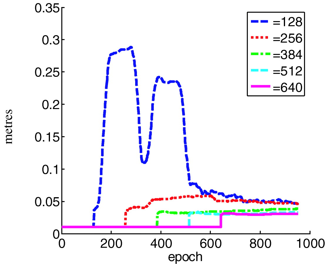
The covariance of observation error R is estimated using different window sizes, as illustrated in Figure 2. All estimates converged to a value of about 0·05 m. The estimation oscillation becomes obvious when shorter window sizes are used, such as 128. This confirms the earlier analysis that a short window size may lead to unstable estimation. The step jumps of the estimation are due to the switch over from the initial settings to the online estimation.

Figure 2. Influence of different window sizes on R estimation.
Assuming precise a priori knowledge is not available, the initial values of R can be defined approximately. Figure 3 shows that different initial values of Q and R have only impacts on the transition period of the estimations. The initial deviations are damped out quickly and the estimation converges with time. The stringent requirements on precise a priori knowledge of the stochastic model have thus been alleviated.

Figure 3. Influence of biased initial values on R estimation (Top left) SQRT of R(1,1) (Top right) SQRT of R(2,2) (Bottom) SQRT of R(3,3).
Since the errors are estimated by the Kalman filter in a GPS/INS integrated system, if the whole system was perfectly modelled and the estimation was optimal and stable, the series of state estimations should be zero-mean white noise series with the minimum covariance. The state estimation STDs have been plotted in Figure 4 against the window sizes used for estimation. Window size zero indicates the conventional KF solution. The STDs are generally smaller when the adaptive estimation method has been used.

Figure 4. Comparison of filtering performance with different window sizes (Top left) position (Top right) velocity (Bottom) attitude.
3.3. Evaluation of the proposed adaptive algorithm
Figure 5 shows the RMSs of the adaptive Kalman filter's states derived from the covariance matrix k. Only the RMS values of the first three diagonal elements have been shown. The trends for the remaining states are similar. It is clear that the overall filter operation is stable and converged. The “bump” at about 100 epochs is caused by the switch to the adaptive algorithm. The window size used for the innovation covariance calculation is 64.

Figure 5. RMS of the adaptively estimated Kalman filter states.
Figure 6 shows the histogram of the estimated scaling factor with time. As expected, after the transition period the scaling factor quickly settles to a value of about one.

Figure 6. The estimated scaling factor sequence.
For the optimal Kalman filter, both innovation and residual magnitudes should be minimised. Figure 7(Left) shows that the magnitude of the innovations is within 0·1 m. After measurement update, the magnitude of the residuals is within 0·02 m, as illustrated in Figure 7(Right). Since the necessary and sufficient condition for the optimality of a Kalman filter is that the innovation sequence should be white, the autocorrelation of the innovation sequence is plotted in Figure 8, which clearly shows white noise features. A further check of the whiteness can be carried out using the method introduced by Mehra (Reference Mehra1970).

Figure 7. (Left) Innovation sequence (Right) Residual sequence.

Figure 8. Autocorrelation of innovation sequence (unbiased).
Figures 9 and 10 show two groups of accelerometer bias and gyro bias estimates for comparison purposes. The process noise parameters used by the conventional extended Kalman filter are calculated according to the manufacturer's technical specification. It can be seen that all three configurations have generated similar estimates. The conventional extended Kalman filter provides the smoothest estimation. The estimates using the process scaling method are much noisier, which may be due to its quick response to signal changes. The estimates on the Z axis have the worst consistency. This may be due to its weak observability, since during the ground vehicle tests the Z axis has the least dynamics. Another reason could be that gravity uncertainties were not properly scaled. They may behave differently from the INS noises.

Figure 9. Estimates of accelerometer bias using different methods: (Top left) Standard Extended KF (Top right) Extended KF with online stochastic modelling (bottom) Extended KF with the proposed process scaling algorithm.

Figure 10. Estimates of gyro bias using different methods: (Top left) Standard Extended KF (Top right) Extended KF with online stochastic modelling (Bottom) Extended KF with the proposed process scaling algorithm.
4. Conclusion
Over the past few decades adaptive KF algorithms have been intensively investigated with a view to reducing the influence of the uncertainty of the covariance matrices of the process noise (Q) and the observation errors (R). The covariance matching method is one of the most promising techniques.
The online adaptive stochastic modelling method provides estimates of individual Q and R elements. However, practical implementation of an online stochastic modelling algorithm faces many challenges. One critical factor influencing the stochastic modelling accuracy is ensuring precise and smooth estimation of the innovation and residual covariances from data sets with limited length. Furthermore, the stochastic parameters are closely correlated with each other when using current estimation algorithms, which make correct estimation more difficult. The online adaptive stochastic modelling method is not scalable for the estimation of a large number of parameters.
In this paper, a new covariance-based adaptive process noise scaling method has been proposed and tested. This method is reliable, robust, and suitable for practical implementations. Initial tests have demonstrated significant improvements of the filtering performance. However, the optimal allocation of noise to each individual source is not possible using scaling factor methods. This is a topic for further investigation.
ACKNOWLEDGEMENT
This research is supported by the Australian Cooperative Research Centre for Spatial Information (CRC-SI) under project 1·3 ‘Integrated positioning and geo-referencing platform’.