2.1. Problem formulation

The subsequent analysis is based on data of highly resolved DNSs of temporally evolving planar jet flows at different Reynolds numbers. The DNS solves the incompressible Navier–Stokes equations in non-dimensional form, given by

(2.1)\begin{equation} \left.\begin{gathered} \frac{\partial U_k}{\partial x_k}=0 , \\ \frac{\partial U_j}{\partial t}+U_k\frac{\partial U_j}{\partial x_k} ={-}\frac{\partial P}{\partial x_j}+ \frac{1}{\mathit{Re}_0} \frac{\partial^2 U_j}{\partial x_k \partial x_k}, \quad j=1,2,3, \end{gathered}\right\} \end{equation}

where $\boldsymbol {U}$ denotes the velocity vector with components $(U_1,U_2,U_3)^\intercal$ in the streamwise, spanwise and cross-wise directions, respectively, and $P$ is the pressure. The corresponding fluctuating fields will be denoted by $\boldsymbol {u} = (u_1,u_2,u_3)^\intercal$ and $p$. The dependent variables are functions of space $\boldsymbol {x}=(x_1,x_2,x_3)^\intercal$ and time $t$. Further, Einstein's summation convention is used, which implies summation over indices appearing twice. All quantities are non-dimensionalized by the initial centreplane mean velocity $U_0$ and the initial jet thickness $H_0$. The jet thickness $H_0$ is defined as the distance over which the mean velocity profile decreases to half of its centreplane value. Without loss of generality, $H_0$ and $U_0$ are set to unity. The initial Reynolds number is defined as

(2.2)\begin{equation} \mathit{Re}_0 = \frac{U_0 H_0}{\nu}, \end{equation}

with $\nu$ being the kinematic viscosity. Four different jet flows with $\mathit {Re}_0$ chosen as 1000, 2000, 5000 and 10 000 are studied in this paper.

The DNS was carried out on the supercomputer JUQUEEN (Stephan & Docter Reference Stephan and Docter2015) with the in-house solver psOpen (Gauding et al. Reference Gauding, Wick, Pitsch and Peters2014, Reference Gauding, Wang, Goebbert, Bode, Danaila and Varea2019; Hunger, Gauding & Hasse Reference Hunger, Gauding and Hasse2016; Sadeghi et al. Reference Sadeghi, Oberlack and Gauding2018). In order to obtain a high accuracy, spatial derivatives are computed by a sixth-order Padé scheme with spectral-like accuracy (Lele Reference Lele1992). Temporal integration is performed by a low storage, stability-preserving fourth-order Runge–Kutta scheme. The Poisson equation is efficiently solved in spectral space by employing a Helmholtz equation (Mellado et al. Reference Mellado, Stevens, Schmidt and Peters2010; Mellado & Ansorge Reference Mellado and Ansorge2012). To reduce aliasing errors, the nonlinear terms are formulated in skew-symmetric form (Erlebacher et al. Reference Erlebacher, Hussaini, Kreiss and Sarkar1990), and additionally, a sixth-order compact filter is applied.

The rectangular computational domain has periodic boundary conditions in the streamwise and spanwise directions (denoted by $x_1$ and $x_2$), and free-slip boundary conditions in cross-wise direction (denoted by $x_3$). The jet flow is statistically homogeneous in the $(x_1,x_2)$-planes, and the jet grows with time $t$ in the cross-wise direction $x_3$. Statistics are computed over $(x_1,x_2)$-planes and depend only on time and the cross-wise coordinate $x_3$. Furthermore, statistical symmetry with respect to the midplane is exploited to improve the quality of statistical quantities. Ensemble averages computed over these planes are denoted by angular brackets. The statistical quality of ensemble averages is discussed in Appendix A.

The governing equations are solved in a computational domain of size $L_{1}/H_0 = 20$, $L_{2}/H_0 = 20$ and $L_{3}/H_0 = 12$, discretized on a mesh with up to $5376 \times 5376 \times 2688$ grid points. The size of the computational domain is sufficiently large compared with the integral scales, firstly, to avoid confinement effects when the thickness of the jet increases with time, and secondly, to improve the quality of statistical quantities. A uniform equidistant mesh is used for the inner part of the domain, while the outer part is increasingly coarsened toward the boundaries. The grid width is chosen such that it is everywhere smaller than the Kolmogorov length scale. This feature of the DNS is especially important for the accurate evaluation of higher-order statistics in the dissipative range (Watanabe & Gotoh Reference Watanabe and Gotoh2007).

An appropriate initialization of the DNS is necessary. Following da Silva & Pereira (Reference da Silva and Pereira2008), the initial velocity profile is composed of two mirrored hyperbolic-tangent mean profiles and perturbed by broadband random Gaussian fluctuations that follow a prescribed energy spectrum. The turbulent intensity $u'/U_0$, with $u'$ being the root mean square of the velocity, equals approximately 2 % to facilitate a rapid transition to fully developed turbulence.

2.2. Characteristic properties of the DNS

The turbulent jet flows used in this study are now briefly characterized. The analysis is carried out for four different jet Reynolds numbers between 1000 and 10 000 (denoted by cases A to D). The case D with the highest Reynolds number is taken as reference case, which is additionally studied at five different times (denoted by D1 to D5). The analysis is conducted in the far field of the jet for $t$ between $t=13.2$ and $t=23.3$. Characteristic parameters of the DNS are summarized in tables 1 and 2.

Table 1. Characteristic properties of four different jet flows (denoted by cases A–D) at time $t=23.3$ with Reynolds numbers $\mathit {Re}_0$ between 1000 and 10 000. Here, $\mathit {Re}_\lambda$ refers to the Taylor-based Reynolds number at the centreplane.

Table 2. Characteristic properties of case D ($\mathit {Re}_0=10\,000$) at the centreplane at five different times (denoted by D1–D5) displayed in figure 1.

In the remainder of this section, we present the temporal evolution of different statistics at the centreplane. Figure 1 displays for case D the evolution of the mean kinetic energy $\langle {k}\rangle =\langle {u_i^2}\rangle /2$ and the mean dissipation rate $\langle {\varepsilon }\rangle =2 \nu \langle {S_{ij} ^2}\rangle$, with

(2.3)\begin{equation} S_{ij} = \frac{1}{2} \left( \dfrac{\partial u_i}{\partial x_j} + \dfrac{\partial u_j}{\partial x_i}\right) \end{equation}

being the strain-rate tensor. It can be observed that $\langle {k}\rangle$ and $\langle {\varepsilon }\rangle$ reveal a power-law decay with scaling exponents close to $-$1 and $-$2, respectively, which is consistent with analytical solutions for complete self-similarity (Gonzalez & Fall Reference Gonzalez and Fall1998; Sadeghi et al. Reference Sadeghi, Oberlack and Gauding2018). To proceed further, let $u_k=(\nu \langle {\varepsilon }\rangle )^{1/4}$ denote the Kolmogorov velocity and $u'=(2 \langle {k}\rangle /3)^{1/2}$ the root mean square of the velocity. From these velocity scales, the Taylor-scale Reynolds number

(2.4)\begin{equation} \mathit{Re}_\lambda = \sqrt{15} \frac{u'^2}{u_k^2} \end{equation}

can be built. The Taylor-scale Reynolds number approaches approximately a constant value, which is between 35 and 107 for the four different simulations considered. In Appendix B, we demonstrate that a constant Reynolds number is a necessary condition for the self-similarity of jet flows.

Figure 1. (a) Temporal evolution of the mean turbulent kinetic energy $\langle {k}\rangle$ as well as the mean energy dissipation rate $\langle {\varepsilon }\rangle$ at the centreplane for case D. The black dashed lines indicate a power-law decay with $t^{-1}$ and $t^{-2}$, respectively. (b) Temporal evolution of the Taylor micro-scale-based Reynolds number $\mathit {Re}_\lambda$ for cases A–D. The circles specify different times (D1–D5) that are used for the self-preservation analysis. The squares represented additional data used to study the variation of the jet Reynolds number $\mathit {Re}_0$.

With a constant Reynolds number, all length and velocity scales follow exactly the same scaling during the decay. Figure 2 shows the temporal evolution of the jet half-width $h_{1/2}$ (defined as the distance from the centreplane over which the mean streamwise velocity decreases to the half of the centreplane value $U_c$), the Taylor micro-scale $\lambda =(15\nu u'^2/\langle {\varepsilon }\rangle )^{1/2}$, the Kolmogorov length scale $\eta =(\nu ^3/\langle {\varepsilon }\rangle )^{1/4}$ as well as the velocity scales $U_{c}$, $u'$ and $u_k$. It can be observed that the length scales increase as $t^{1/2}$, and at the same time, the velocity scales decrease as $t^{-1/2}$. Also, the outer scales $h_{1/2}$ and $U_{c}$ follow the same scaling laws, see Appendix B for the derivation.

Figure 2. (a) Temporal evolution of the length scales $h_{1/2}$, $\lambda$ and $\eta$ (a), where the dashed lines indicate the self-similarity solution with $t^{1/2}$, and (b) temporal evolution of the velocity scales $U_{c}$, $u'$ and $u_k$, where the dashed lines represent the self-similarity solution with $t^{-1/2}$. The circles indicate different times that are used for the further analysis. Data presented for case D.

3.1. Analytical similarity solutions of structure functions

Analytical solutions of structure functions exist in the asymptotic small-scale and large-scale limits and can be used to derive conditions for self-similarity and self-preservation. In the small-scale limit, a Taylor series expansion of $\langle {\Delta u_1^{2n}}\rangle$ gives

(3.3)\begin{equation} \langle{\Delta u_1^{2n}}\rangle = \left\langle{\left( \dfrac{\partial u_1}{\partial x_1}\right)^{2n}}\right\rangle r^{2n} + {O} (r^{2n+2}) , \end{equation}

where the series is truncated after the first non-negative term. Normalizing (3.3) with the Kolmogorov scales gives the expression

(3.4)\begin{equation} \frac{\langle{\Delta u_1^{2n}}\rangle}{u_k^{2n}} = \frac{F^<_{2n} R_\varepsilon}{15^n} \left(\frac{r}{\eta} \right)^{2n}. \end{equation}

The right-hand side of (3.4) depends on two external parameters, $F^<_{2n}$ and $R_\varepsilon$, as well as the universal shape function $(r/\eta )^{2n}$. The first external parameter in (3.4) is the non-dimensional moment of the streamwise velocity gradient

(3.5)\begin{equation} F^<_{2n} = \frac{\left\langle{\left( \dfrac{\partial u_1}{\partial x_1} \right)^{2n}}\right\rangle}{\left\langle{\left( \dfrac{\partial u_1}{\partial x_1} \right)^2}\right\rangle^n} , \end{equation}

which quantifies intermittent fluctuations of the velocity gradient field (Frisch Reference Frisch1995; Sreenivasan & Antonia Reference Sreenivasan and Antonia1997). The second parameter

(3.6)\begin{equation} R_\varepsilon= \frac{15 \nu}{\langle{\varepsilon}\rangle} \left\langle{\left( \dfrac{\partial u_1}{\partial x_1}\right)^2}\right\rangle \end{equation}

quantifies the departure from small-scale isotropy and equals unity under local isotropy. Equation (3.4) is an exact generalization of Kolmogorov's first scaling hypothesis (Kolmogorov Reference Kolmogorov1941b) to anisotropic turbulence with internal intermittency (Boschung et al. Reference Boschung, Hennig, Gauding, Pitsch and Peters2016). Alternatively, structure functions can be normalized with the Taylor scales $u'$ and $\lambda$, which gives with (3.3) the expression

(3.7)\begin{equation} \frac{\langle{\Delta u_1^{2n}}\rangle}{u'^{2n}} = {F^<_{2n} R_\varepsilon} \left( \frac{r}{\lambda} \right)^{2n}. \end{equation}

Essentially, (3.4) and (3.7) are analytical solutions for $\langle {\Delta u_1^{2n}}\rangle$ in the dissipative range that account for both anisotropy and intermittency. Independent of the chosen set of length and velocity scales, self-preservation of structure functions at the small scales requires that the product of $F^<_{2n}$ and $R_\varepsilon$ is invariant with time (note that $F^<_2$ equals unity, and hence the constancy of $R_{\varepsilon }$ is sufficient for the second order).

Analytical solutions for structure functions also exist in the large-scale limit. In statistically homogeneous turbulence, structure functions become independent of the separation distance when $r$ is larger than the integral length scale. The limiting value can be obtained from the binomial theorem and equals

(3.8)\begin{equation} \langle{\Delta u_1^{2n}}\rangle = \sum_{k=0}^{2n} {{2n} \choose {k}} ({-}1)^k \langle{u_1^{2n-k}}\rangle\langle{u_1^k}\rangle. \end{equation}

To proceed, we exploit the fact that all odd moments of $u_1$ vanish at the centreplane due to symmetry. In that case, (3.8) simplifies to

(3.9)\begin{equation} \langle{\Delta u_1^{2n}}\rangle = \sum_{k=0}^n \frac{(2n)!}{(2k)! (2n-2k)!} \langle{u_1^{2n-2k}}\rangle \langle{u_1^{2k}}\rangle. \end{equation}

By introducing the non-dimensional moments of the velocity fluctuations

(3.10)\begin{equation} F^>_{2n} = \frac{\langle{u_1^{2n}}\rangle}{\langle{u_1^2}\rangle^n}. \end{equation}

Equation (3.9) can be rewritten as

(3.11)\begin{equation} \langle{\Delta u_1^{2n}}\rangle = \langle{u_1^2}\rangle^n \sum_{k=0}^n \frac{(2n)!}{(2k)! (2n-2k)!} F_{2n-2k}^> F_{2k}^>{=} \langle{u_1^2}\rangle^n C_{2n}, \end{equation}

where the prefactor $C_{2n}$ relates the large-scale limit of any order structure function to the variance $\langle {u_1^2}\rangle$. For instance, from (3.11) we find that $\langle {\Delta u_1^2}\rangle$ approaches $2 \langle {u_1^2}\rangle$, and $\langle {\Delta u_1^4}\rangle$ approaches $2(F_{4}^>+3) \langle {u_1^2}\rangle ^2$. Further, we introduce a large-scale anisotropy parameter $R_u$ as

(3.12)\begin{equation} \langle{u_1^2}\rangle = R_u u'^2 , \end{equation}

which equals unity for isotropic turbulence. With these definitions, the large-scale limit of $\langle {\Delta u_1^{2n}}\rangle$ becomes, after normalization with the Kolmogorov scales,

(3.13)\begin{equation} \frac{\langle{\Delta u_1^{2n}}\rangle}{u_k^{2n}} = 15^{{-}n/2} C_{2n} R_u^n \mathit{Re}_\lambda^n, \end{equation}

and after normalization with the Taylor scales

(3.14)\begin{equation} \frac{\langle{\Delta u_1^{2n}}\rangle}{u'^{2n}} = C_{2n} R_u^n. \end{equation}

Self-preservation of the structure functions at the large scales requires hence the constancy of the right-hand sides of (3.13) and (3.14).

The analysis presented provides certain constraints for self-preservation that structure functions of different order must satisfy. For second-order structure functions, the only requirement for self-preservation is the constancy of the anisotropy factors $R_u$ and $R_\varepsilon$ during the evolution of the jet as $F^<_2$ and $F^>_2$ equal unity by definition, see (3.4), (3.7), (3.13) and (3.14). An important consequence is that isotropy is not required for the validity of self-preservation and any anisotropy that is present in the flow must persist indefinitely. In other words, a return to isotropy is not consistent with self-preservation. The persistence of anisotropy has been also postulated in the context of self-similarity of turbulent wakes by Thiesset, Danaila & Antonia (Reference Thiesset, Danaila and Antonia2013b).

Knowing that the anisotropy factors $R_u$ and $R_\varepsilon$ must stay constant for self-preservation, the analysis provides additional constraints for higher-order structure functions. More specifically, (3.4), (3.7), (3.13) and (3.14) require that the non-dimensional moments $F^<_{2n}$ and $F^>_{2n}$ remain constant for self-preservation. This condition is valid for any even order. It should be noted that the constancy of the flatness factors can be also inferred from the constancy of the Reynolds number (Schumacher et al. Reference Schumacher, Scheel, Krasnov, Donzis, Yakhot and Sreenivasan2014) in completely self-preserving flows.

Table 3 lists for case D the aforementioned parameters at the centreplane during the evolution of the jet. The flatness factor $F^>_{4}$ is close to 2.9, which indicates that velocity fluctuations in the core of the jet follow approximately a Gaussian distribution. The flatness of the velocity gradients $F^<_4$ is close to 6, which reflects departures from Gaussianity due to intermittency. Table 3 shows that the anisotropy factors $R_u$ and $R_\varepsilon$ also stay nearly constant during the decay of the jet. Small-scale isotropy is fulfilled within less than two per cent deviation, while the departure from large-scale isotropy reaches approximately ten per cent. Furthermore, table 3 shows that the skewness of the velocity fluctuations, defined as $S_u=\langle {u_1^3}\rangle /\langle {u_1^2}\rangle ^{3/2}$, remains close to zero at the centreplane, as required by symmetry.

Table 3. Temporal evolution of different quantities at the centreplane of case D, i.e. the velocity gradient flatness $F^<_4$, the flatness of the velocity fluctuations $F^>_4$, the skewness of the velocity fluctuations $S_u=\langle {u_1^3}\rangle /\langle {u_1^2}\rangle ^{3/2}$ as well as the anisotropy coefficients $R_\varepsilon$ and $R_u$, characterizing the small- and large-scale anisotropy, respectively.

3.2. Self-preservation of structure functions at the centreplane

Let us now examine whether structure functions are self-preserving at the centreplane. The analysis is conducted for the even-order longitudinal structure functions up to the sixth order. Higher-order structure functions are of interest because they provide information about intermittency (Pearson & Antonia Reference Pearson and Antonia2001). The characteristic scales $u_{ref}$ and $L_{ref}$ are chosen as (1) the Kolmogorov scales $u_k$ and $\eta$, (2) the Taylor scales $u'$ and $\lambda$ and (3) the outer scales $U_{c}$ and $h_{1/2}$. Once the jet flow has reached a constant Reynolds number, the inner scales (Kolmogorov or Taylor scales) should be exchangeable with the outer scales ($U_{c}$ and $h_{1/2}$). This assertion is tested now using the DNS data.

Figure 3 shows $f_2(\hat r)$, $f_4(\hat r)$ and $f_6(\hat r)$ at the centreplane ($\hat x_3=0$) for $\mathit {Re}_0=10\,000$ at five different times (D1–D5). It can be seen that the normalized structure functions admit complete self-preservation, which means that the normalized structure functions collapse for any time $t$ over the entire $r$ space. Hence, complete self-preservation is valid regardless of the order and the chosen set of reference scales. It should be mentioned that complete self-preservation of second-order structure functions has also been reported by Tang et al. (Reference Tang, Antonia, Djenidi and Zhou2016) and Thiesset et al. (Reference Thiesset, Antonia and Djenidi2014a) at the centre of round jets.

Figure 3. Self-preservation of even-order structure functions up to the sixth order at the centre of the jet ($\hat x_3=0$). The structure functions are normalized by the Kolmogorov scales (1), the Taylor scales (2) and the outer scales (3) and presented at different times (D1–D5).

Complete self-preservation is a direct consequence of the constant centreplane Reynolds number. At a constant Reynolds number, the ratio between large-scale and small-scale quantities remains unchanged with time and any set of length and velocity scales can be chosen as reference scales. In that case, self-preservation of structure functions is not only valid for the second order but valid for any higher order.

3.3. Self-preservation of structure functions in the shear region

At the centre of the jet, turbulence statistics are close to those observed in homogeneous isotropic decaying turbulence (Antonia et al. Reference Antonia, Smalley, Zhou, Anselmet and Danaila2003; Sinhuber, Bodenschatz & Bewley Reference Sinhuber, Bodenschatz and Bewley2015). In this section, we examine whether structure functions still admit complete self-preservation away from the centre of the jet, where turbulence is affected by a mean shear or inhomogeneity and anisotropy effects (Casciola et al. Reference Casciola, Gualtieri, Benzi and Piva2003; Thiesset et al. Reference Thiesset, Schaeffer, Djenidi and Antonia2014b).

To this end, we examine the self-preservation of the normalized structure functions in the shear layer of the jet at the position $x_3=h_{1/2}$. At this position, the mean shear ${\partial \langle {U_1}\rangle }/{\partial x_3}$ is close to its maximum. Figure 4 presents for case D the corresponding structure functions up to the sixth order after normalization with the Kolmogorov scales (1), the Taylor scales (2) and the outer scales (3). Again, a perfect collapse can be observed over the entire range of scales for each order, regardless of the chosen set of scales for normalization. Hence, by comparison with figure 3, we can conclude that complete self-preservation of structure functions is not limited to the core of the jet, but also valid in the shear layer.

Figure 4. Self-preservation of even-order structure functions up to the sixth order at the edge of the jet at $x_3=h_{1/2}$. At this position, the mean shear ${\partial \langle {U_1}\rangle }/{ \partial x_3}$ is close to its maximum. The structure functions are normalized by the Kolmogorov scales (1), the Taylor scales (2) and the outer scales (3) and presented at different times (D1–D5).

3.4. Impact of the initial conditions on the self-similarity of structure functions

In the spirit of Kolmogorov's similarity theory, it is of interest to study the influence of a variation of the jet Reynolds number $\mathit {Re}_0$ on the self-similarity of the structure functions. To this end, we examine whether the normalized structure functions $S_n(\hat r;t,\hat x_3,\mathit {Re}_0)/u_{ref}^n(t,\hat x_3,\mathit {Re}_0)$ collapse over the entire $r$ space when the jet Reynolds number $\mathit {Re}_0$ is changed and the other parameters are kept constant. To answer this question, we examine different jet flows with variations of the Reynolds number $\mathit {Re}_0$ between 1000 and 10 000, cf. table 1.

Figure 5 presents the second-order structure functions for these different jet Reynolds numbers at the centreplane. As expected, the structure functions do not satisfy self-similarity over the entire range of scales, neither after normalization with the Kolmogorov scales nor with the Taylor scales. Instead, the collapse with the Kolmogorov scales is restricted to the dissipative range, while the Taylor scales lead to a collapse only in the dissipative range and at the large scales, but not at intermediate scales. This finding confirms the standard understanding of turbulence that, in general, and specifically at low to moderate Reynolds numbers, structure functions do not feature universality over the entire range of scales (Pearson & Antonia Reference Pearson and Antonia2001). Moreover, figure 5 supports the claim that a constant turbulent Reynolds number is a necessary condition for complete self-similarity or self-preservation of structure functions.

Figure 5. Normalized second-order structure functions at the centreplane for different Reynolds numbers between 1000 and 10 000. The structure functions are normalized by Kolmogorov scales (a) and Taylor scales (b).

It is important to note that by virtue of self-preservation, the results presented are invariant with time once the far field of the jet is reached.

4.1. The TNTI

External intermittency can be evaluated by the intermittency – or indicator – function $\varGamma$, defined as

(4.1)\begin{equation} \varGamma(\boldsymbol{x},t) = {H(\omega^2(\boldsymbol{x}, t)-\omega^2_0)} , \end{equation}

where $H$ is the Heaviside function, $\omega ^2$ is the enstrophy and $\omega ^2_0$ is a threshold value of the enstrophy that defines the position of the IB. The intermittency factor

(4.2)\begin{equation} \gamma(x_3,t) = \langle{\varGamma(\boldsymbol{x},t)}\rangle , \end{equation}

quantifies the probability that the flow at a certain cross-wise position $x_3$ is turbulent (Townsend Reference Townsend1949). Since the IB is a singular surface, the flow field can be partitioned into two states, either turbulent if $\omega ^2>\omega ^2_0$, or non-turbulent in any other case. With this definition, any conventionally averaged quantity $\langle {\varPsi }\rangle$ can be decomposed as

(4.3)\begin{equation} \langle{\varPsi}\rangle = \gamma \langle{\varPsi}\rangle_t + (1-\gamma) \langle{\varPsi}\rangle_{n}, \end{equation}

where $\langle {\varPsi }\rangle _t$ and $\langle {\varPsi }\rangle _n$ indicate conditional averages that consider either turbulent and non-turbulent events, respectively (Mellado, Wang & Peters Reference Mellado, Wang and Peters2009). With the binary indicator function $\varGamma$, the conditional averages are defined as

(4.4a,b)\begin{equation} \langle{\varPsi}\rangle_t = \langle{\varGamma \varPsi}\rangle \quad \text{and} \quad \langle{\varPsi}\rangle_n = \langle{(1-\varGamma) \varPsi}\rangle. \end{equation}

It is now widely accepted that the IB can be defined by an appropriate threshold of the enstrophy (Bisset, Hunt & Rogers Reference Bode, Gauding, Lian, Denker, Davidovic, Kleinheinz, Jitsev and PitschReference Bisset, Hunt and Rogers2002; Holzner et al. Reference Holzner, Liberzon, Nikitin, Lüthi, Kinzelbach and Tsinober2008; da Silva & Pereira Reference da Silva and Pereira2008; da Silva et al. Reference da Silva, Hunt, Eames and Westerweel2014; Silva et al. Reference Silva, Zecchetto and da Silva2018; Watanabe, da Silva & Nagata Reference Watanabe, da Silva and Nagata2019). The threshold value $\omega ^2_0$ is systematically obtained from the probability density function (p.d.f.) of $\log _{10}(\omega ^2/\hat \omega ^2)$. Following Krug et al. (Reference Krug, Chung, Philip and Marusic2017a), the local enstrophy field is normalized by $\hat \omega ^2$, defined as

(4.5)\begin{equation} \hat \omega^2 = \frac {\displaystyle\int_{-\infty}^{\infty} \langle{\omega^2}\rangle^2 \,\textrm{d} x_3 } {\displaystyle\int_{-\infty}^{\infty} \langle{\omega^2}\rangle \,\textrm{d}x_3} , \end{equation}

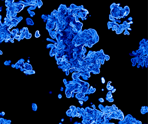
to remove the time dependence from the threshold criterion. Figure 6(a) displays the p.d.f. of $\log _{10}(\omega ^2/\hat \omega ^2)$ at different times. In flows exposed to external intermittency, the p.d.f. exhibits a bimodal shape, where the two peaks that represent turbulent and non-turbulent regions are clearly separated by several orders of magnitude. In this work, we chose a threshold $\log _{10}(\omega _0^2/\hat \omega ^2)=-3.4$ for all cases. The enstrophy sharply increases across the TNTI, which makes the position of the IB reasonably insensitive regarding the exact threshold value (Krug et al. Reference Krug, Holzner, Marusic and van Reeuwijk2017b; Elsinga & da Silva Reference Elsinga and da Silva2019). The visualization of the enstrophy field and the IB in figure 7 indicates that the threshold is suitably chosen to distinguish between turbulent and non-turbulent regions. Furthermore, the sensitivity of the reported results with respect to the value of the threshold is examined in Appendix A.

Figure 6. (a) The p.d.f. of $\log _{10}(\omega ^2/\hat \omega ^2)$ at different times for case D. The dashed vertical line indicates the threshold $\log _{10}(\omega _0^2/\hat \omega ^2)=-3.4$. (b) Variation of the intermittency factor $\gamma$ with the cross-wise coordinate $\hat x_3$ at different times (D1–D5) and jet Reynolds numbers $\mathit {Re}_0$ between 1000 and 10 000 (inset).

Figure 7. Visualization of the enstrophy field $\omega ^2/\hat \omega ^2$ for case D5 in a $(x_1,x_3)$-plane. The black contour line represents the IB defined by the enstrophy criterion $\log _{10}(\omega _0^2/\hat \omega ^2)=-3.4$.

Figure 6(b) shows the variation of the intermittency factor $\gamma$ with the cross-wise coordinate $\hat x_3$ for different time steps and Reynolds numbers. At the centre, there is an almost fully turbulent region with $\gamma$ close to unity that extends up to $\hat x_3 \approx 0.5$. At the edge of the flow, a steep decrease of $\gamma$ is visible. It originates from an alternating flow structure, when the outer fluid with low vorticity is mixed with highly turbulent fluid from the core region of the jet. A visualization of this flow structure is shown in Appendix C. It is also worth mentioning that $\gamma$ is approximately self-preserving and independent of the Reynolds number when plotted as a function of $\hat x_3$.

In the next section, the intermittency structure function is introduced to evaluate the morphology of the IB at different scales.

4.2. Intermittency structure function

In turbulent flows exposed to external intermittency, there are three different possibilities for the distribution of the ending points $\boldsymbol {x}$ and $\boldsymbol {x} + r \boldsymbol {e}_1$ of the velocity increments $\Delta u_1=u_1(\boldsymbol {x} + r \boldsymbol {e}_1,t) - u_1(\boldsymbol {x},t)$ along a straight line. More precisely, both points can be either located within the turbulent or within the non-turbulent regime or one point may be in the turbulent and the other point in the non-turbulent regime. Kuznetsov et al. (Reference Kuznetsov, Praskovsky and Sabelnikov1992) predicted the corresponding probabilities as $\gamma _{tt}=\gamma - \frac {1}{2} D_{\varGamma ,IB}$, $\gamma _{nn}= 1 - \gamma - \frac {1}{2} D_{\varGamma ,IB}$ and $\gamma _{nt}=D_{\varGamma ,IB}$, where

(4.6)\begin{equation} D_{\varGamma,IB}(r;x_3,t) = \langle{(\varGamma(\boldsymbol{x} + r \boldsymbol{e}_1,t) - \varGamma(\boldsymbol{x},t) )^2}\rangle \end{equation}

is the intermittency structure function. The probabilities satisfy the identity

(4.7)\begin{equation} \gamma_{tt} + \gamma_{nn} + \gamma_{nt} =1. \end{equation}

The ratio

(4.8)\begin{equation} \frac{\gamma_{tt}}{\gamma} = 1 - \frac{D_{\varGamma,IB}}{2 \gamma} \end{equation}

measures the conditional probability that one point of the increment

(4.9)\begin{equation} \Delta \varGamma =\varGamma(\boldsymbol{x} + r \boldsymbol{e}_1,t) - \varGamma(\boldsymbol{x},t) \end{equation}

is in the turbulent regime given that the other point is also in a turbulent regime. In other words, $D_{\varGamma ,IB}$ provides scale-sensitive information regarding the structure of the IB. Figure 8(a) shows $\gamma _{tt}/\gamma$ at different cross-wise positions $\hat x_3$ varying between the centreplane and $\hat x_3=1.59$ for case D5 as a representative case. It can be observed that in the proximity of the centreplane (i.e. for $0 \le \hat x_3 \le 0.58$), $\gamma _{tt}/\gamma$ is close to unity and nearly independent of the separation distance $r$, which reflects the fact that the core region of the jet is fully turbulent. Toward the edge of the jet, $\gamma _{tt}/\gamma$ equals unity only for $r\to 0$, and decreases quickly at larger separation distances. This decrease comes from the alternation between turbulent and non-turbulent fluid and represents external intermittency.

Figure 8. (a) Conditional probability $\gamma _{tt}/\gamma$ at different cross-wise positions $\hat x_3$ (as indicated in the legend, $\hat x_3=0$ represents the centreplane). (b) Comparison of the structure function $D_{\varGamma ,T}$ of a random telegraphic function (green dashed lines) with the intermittency structure function $D_{\varGamma ,IB}$, shown for two different cross-wise positions $\hat x_3$ (solid red and blue lines). The black dashed lines indicate the analytical small-scale and large-scale limits. Data for case D5.

To proceed further, we introduce the one-dimensional random telegraphic signal $\varGamma _T$ as a model for the intermittency function $\varGamma$. The telegraphic signal $\varGamma _T$ alternates randomly between 0 (non-turbulent) and 1 (turbulent) and the corresponding probabilities are defined as $p(\varGamma _T=0)=1-\gamma$ and $p(\varGamma _T=1)=\gamma$. Thiesset et al. (Reference Thiesset, Duret, Ménard, Dumouchel, Reveillon and Demoulin2020) showed that the random telegraphic signal has an analytical structure function, i.e.

(4.10)\begin{equation} D_{\varGamma,T}(r) = 2 \gamma ( 1-\gamma ) [ 1 - \textrm{e}^{{-}r/\mathcal{L}_T}] , \end{equation}

where $\mathcal {L}_T$ is a characteristics length scale

(4.11)\begin{equation} \mathcal{L}_T = 2 \gamma ( 1-\gamma ) \left[\lim_{r\to 0} \frac{D_{\varGamma,T}(r)}{r} \right]^{{-}1} , \end{equation}

which is related to the probability for a transition from 0 to 1 and vice versa (Fitzhugh Reference Fitzhugh1983). The small-scale limit of the random telegraphic signal equals

(4.12)\begin{equation} \lim_{r \to 0} D_{\varGamma,T}(r) = 2 \gamma ( 1-\gamma) \frac{r}{\mathcal{L}_T} + {O}(r^2) , \end{equation}

which signifies that $D_{\varGamma ,T}$ is proportional to $r$ when the separation distance is small compared with $\mathcal {L}_T$. It is important to note that (4.12) is fundamentally different from the small-scale limit of velocity structure functions where $\langle {\Delta u_1^2}\rangle \propto r^2$ applies. The different scaling is related to the fact that the velocity is a continuous field, while the intermittency function $\varGamma (\boldsymbol {x},t)$ possesses discontinuities.

It is of interest to compare the analytical structure function of the random telegraphic signal $D_{\varGamma ,T}$ with the intermittency structure function $D_{\varGamma ,IB}$ of the turbulent jet. The intermittency structure function $D_{\varGamma ,IB}$ is presented in figure 8(b) for two different cross-wise positions, normalized similar to (4.11) by the characteristic length scale

(4.13)\begin{equation} \mathcal{L}_{IB} = 2\gamma(1-\gamma) \left[ \lim_{r\to 0} \frac{D_{\varGamma,IB}(r;x_3)}{r} \right]^{{-}1} , \end{equation}

and the large-scale limit $2 \gamma (1-\gamma )$. Figure 8(b) reveals a perfect collapse between the DNS data and the random telegraphic function in the small-scale and large-scale limits. For intermediate scales, there is a growing discrepancy between $D_{\varGamma ,T}$ and $D_{\varGamma ,IB}$ with increasing distance from the centreplane. This difference is due to the fact that the morphology of the IB is not fully random, but instead determined by the dynamics of turbulence.

Let us now use the intermittency structure function to further examine the structure of the IB. Following Debye & Bueche (Reference Debye and Bueche1949) and Debye, Anderson & Brumberger (Reference Debye, Anderson and Brumberger1957), the small-scale limit of $D_{\varGamma ,IB}$ can be expressed as

(4.14)\begin{equation} \lim_{r \to 0} \frac{D_{\varGamma,IB}}{r} = \left\langle{ \left| \dfrac{\partial \varGamma}{\partial x_1}\right|}\right\rangle , \end{equation}

where the jump frequency

(4.15)\begin{equation} \varSigma = \left\langle{ \left| \dfrac{\partial \varGamma}{\partial x_1} \right|}\right\rangle = \frac{n_{IB}}{L_1} , \end{equation}

quantifies the number of alternations $n_{IB}$ between turbulent and non-turbulent fluid (and vice versa) per length $L_1$ along a straight line in the streamwise direction. Figure 9(a) shows the jump frequency $\varSigma$ as a function of the cross-wise coordinate $\hat x_3$ at different times. It can be observed that $\varSigma$ is characterized by a single distinct maximum, which identifies the position where the IB is most corrugated. With the spreading of the jet, the maximum decreases and moves outwards in cross-wise direction. After normalization with the half-width $h_{1/2}$, $\varSigma$ admits a self-preserving shape, see figure 9(b). The consequence of self-preservation is that

(4.16)\begin{equation} \frac{n_{IB}}{L_1} \propto h_{1/2}^{{-}1} , \end{equation}

which means that the surface of the IB is smoothed as the jet spreads. This observation is consistent with the growth of the characteristic length scales during the self-similar decay of the jet.

Figure 9. Jump frequency $\varSigma$ as a function of the cross-wise position $x_3$ at different times (a) and self-preservation of $\varSigma$ after normalization with the jet half-width $h_{1/2}$ (b). Data for case D.

Finally, the dependence of the jump frequency $\varSigma$ on the jet Reynolds $\mathit {Re}_0$ is of interest. As shown in figure 10, the location of the maximum of $\varSigma$ remains at approximately $x_3/h_{1/2}=1.4$ despite a variation of $\mathit {Re}_0$ by one decade between 1000 and 10 000. However, the value of the maximum clearly increases with the Reynolds number. This increase originates from smaller turbulent length scales that create a more contorted IB at higher Reynolds numbers. The shape of the jump frequency $\varSigma h_{1/2}$ becomes approximately Reynolds number independent when rescaled with the jet Reynolds number $\mathit {Re}_0^\alpha$, where $\alpha$ is found empirically to be close to $-$0.4.

Figure 10. Jump frequency $\varSigma$ as a function of the cross-wise position $x_3/h_{1/2}$ for different jet Reynolds numbers $\mathit {Re}_0$ between 1000 and 10 000 (a). The jump frequency becomes approximately independent of $\mathit {Re}_0$ when rescaled by $h_{1/2}$ and $\mathit {Re}_0^\alpha$, where $\alpha$ is found empirically to be close to $-$0.4 (b).

4.3. Self-similarity of structure functions along the cross-wise direction

The strong variation of the jump frequency $\varSigma$ along the cross-wise direction raises the question whether structure functions can admit self-similarity when varying the cross-wise location $\hat x_3$ while keeping $\mathit {Re}_0$ and $t$ constant. Figure 11 shows the normalized second, fourth- and sixth-order velocity structure functions $f_n(\hat r,\hat x_3)$ at different cross-wise positions between the centreplane and $\hat x_3=1.59$. The structure functions are normalized by the Kolmogorov scales $\eta$ and $u_k$. For the second order, there is reasonable support for self-similarity with respect to $\hat x_3$, since an adequate collapse of structure functions can be observed. As expected, the collapse is perfect for the smallest scales, where structure functions obey the classical Kolmogorov scaling $\langle {\Delta u_1^2}\rangle /u_k^2 \propto (r/\eta )^2$. At the largest scales, self-similarity still holds with good accuracy despite finite Reynolds number effects.

Figure 11. Normalized even-order velocity structure functions up to the sixth order at different cross-wise positions $\hat x_3$ from the centreplane (red) up to $\hat x_3=1.59$ (blue). The structure functions are normalized by the Kolmogorov scales $u_k$ and $\eta$. For clarity, the fourth-order structure functions and the sixth-order structure functions are shifted upwards by two and four decades, respectively. Data for case D5.

However, the situation is different for the self-similarity of higher-order structure functions. From figure 11, it is evident that the fourth-order and sixth-order structure functions reveal a non-collapsing and clearly non-self-similar arrangement over the entire range of scales. This finding is in line with the standard paradigm that higher-order statistics are non-universal and highly sensitive to different effects, such as intermittency but also finite Reynolds number effects and the associated coupling to the boundary conditions of the flow. But keeping in mind that higher-order structure functions admit complete self-preservation at the centreplane and in the shear layer at fixed $\hat x_3$ (cf. § 3), this finding requires further explanation. The objective of the remainder of the paper is to show that external intermittency plays an important role for the lack of self-similarity of higher-order structure functions.

To visualize the physical mechanism behind the break down of self-similarity, we present in figure 12 the intermittency function $\varGamma$ and the square of the longitudinal velocity gradient $(\partial u_1/\partial x_1)^2$ at different cross-wise positions $\hat x_3$ along a straight line in the streamwise direction $x_1$. At the centreplane, the jet is fully turbulent and large excursions from the mean value of $(\partial u_1/\partial x_1)^2$ occur, which is characteristic of a signal with internal intermittency. These excursions originate from thin, confined layers that are of the order of a few Kolmogorov length scales. Toward the edge of the jet flow, the nature of turbulence changes drastically when external intermittency comes into play. The principal feature of external intermittency is that it imposes external information on the signal. This external information can be quantified statistically at the large scales by the intermittency factor $\gamma$ (ratio between turbulent and non-turbulent regimes) and at the small scales by the jump frequency $\varSigma$ (frequency of the alternation between turbulent and non-turbulent regimes). Both quantities depend on the morphology of the IB with the consequence that turbulence is not self-similar along the $\hat x_3$ direction. This assertion is now supported by a statistical analysis.

Figure 12. Intermittency function $\varGamma$ (a) and the square of the longitudinal velocity gradient $(\partial u_1/\partial x_1)^2$ (b) at different cross-wise positions $x_3$ along a straight line in the streamwise direction $x_1$. The signals are shifted upwards for clarity. Data for case D5 at different cross-wise positions $\hat x_3$ equal to $0.0, 0.29, 0.58, 0.87, 1.15, 1.44$ and $1.59$ (from bottom to top).

Following Frisch (Reference Frisch1995), we define a turbulent signal to be intermittent when it features strong activity only during a fraction of time (or space). To quantify intermittency at different scales, we introduce the relation between structure functions and the p.d.f. of velocity increments $P(\Delta u_1;r,x_3)$,

(4.17)\begin{equation} \langle{\Delta u_1^{n}}\rangle = \int_{-\infty}^\infty \Delta u_1^n P(\Delta u_1;r,x_3)\, \textrm{d} (\Delta u_1). \end{equation}

Equation (4.17) highlights that higher-order moments provide information about the far tails of the p.d.f.  which makes them a suitable tool for the study of intermittency. The shape of the distribution $P(\Delta u_1;r,x_3)$ can be quantified by the flatness factors

(4.18)\begin{equation} F^<_4 = \frac{ \left\langle{\left( \dfrac{\partial u_1}{\partial x_1} \right)^4 }\right\rangle }{ \left\langle{\left( \dfrac{\partial u_1}{\partial x_1} \right)^2 }\right\rangle^2 }, \end{equation}

and

(4.19)\begin{equation} F^>_4 = \frac{ \langle{ u_1^4 }\rangle }{ \langle{u_1^2 }\rangle^2 }, \end{equation}

which represent intermittency at the small scales and large scales, respectively. From the dependence of the velocity gradient flatness $F^<_4$ on the external intermittency factor $\gamma$, the inter-scale coupling of turbulence can be analysed. Figure 13(a) shows that $F^<_4$ increases from a centreplane value close to 6 to a value close to 30 when $\gamma$ equals 0.2. This dependence clearly demonstrates that external intermittency can have a striking impact on the small scales (represented by $F^<_4$), and that the small scales do not decouple from the large scales (represented by $\gamma$). Internal intermittency can be ruled out as the reason for the increase of $F^<_4$ because the turbulent Reynolds number moderately decays toward the edge of the jet. Also, the velocity fluctuation flatness $F^>_4$ increases across the jet from approximately 3 at the centreplane to 10 at $\gamma =0.2$. This means that the assumption of Gaussianity for the velocity fluctuations is valid in the core but not at the edge of the flow. It is also worth noting that the dependence of the flatness factors $F^<_4$ and $F^>_4$ on $\gamma$ appears to be self-preserving.

Figure 13. Flatness factor of the velocity gradients $F^<_4$ and the velocity fluctuations $F^>_4$ as a function of the intermittency factor $\gamma$ at (a) different times (cases D1–D5) and (b) different jet Reynolds numbers (cases A–D). The black dashed line represents the flatness factor of a Gaussian distribution.

In figure 13(b), we present the effect of the jet Reynolds number $\mathit {Re}_0$ on the flatness factors. It can be seen that the flatness factor of the velocity gradients $F_4^<$ increases notably with Reynolds number, but its variation with $\gamma$ is approximately the same for all Reynolds numbers. Based on the concept of scale separation, $F^<_4$ should gradually become less sensitive to external intermittency as the Reynolds number increases. However, this trend is not supported by figure 13(b). An explanation for this observation could be the relatively low Reynolds numbers of the simulations at hand for which no sufficient decoupling between small and large scales exists (Mydlarski & Warhaft Reference Mydlarski and Warhaft1996). Moreover, figure 13(b) indicates that the flatness factor of the velocity fluctuations $F^>_4$ depends only weakly on the jet Reynolds number $\mathit {Re}_0$.

In order to further understand the impact of external intermittency on turbulence, we define conditional flatness factors

(4.20)\begin{equation} F^<_4|_t = \frac{\left\langle{ \varGamma \left( \dfrac{\partial u_1}{\partial x_1} \right)^4 }\right\rangle} {\left\langle{ \varGamma \left( \dfrac{\partial u_1}{\partial x_1} \right)^2 }\right\rangle^2}, \end{equation}

and

(4.21)\begin{equation} F^>_4|_t = \frac{\langle{ \varGamma u_1^4 }\rangle} {\langle{ \varGamma u_1^2 }\rangle^2}, \end{equation}

that consider only the turbulent portion of the jet. Turbulent and non-turbulent regions are distinguished by the intermittency function $\varGamma (\boldsymbol {x})$. Unlike the conventional flatness factors $F^<_4$ and $F^>_4$, figure 14 shows that the conditional flatness factors $F^<_4|_t$ and $F^>_4|_t$ are virtually constant and significantly less sensitive to variations of $\gamma$. This finding is valid independently of the jet Reynolds number and originates from strong turbulent transport that leads in a statistical sense to a rapid homogenization of fully turbulent regions. A rapid homogenization of turbulent regions in free shear flows was already speculated by Corrsin & Kistler (Reference Corrsin and Kistler1955) and later confirmed by Mellado et al. (Reference Mellado, Wang and Peters2009).

Figure 14. (a) Conditional flatness factors $F^<_4|_t$ and $F^>_4|_t$ (solid lines) are approximately independent of the intermittency factor $\gamma$. The flatness factors $F^<_4$ and $F^>_4$ (dashed lines) are shown for comparison. (b) Dependence of $F^<_4|_t$ on the jet Reynolds number. The black dashed line represents the flatness factor of a Gaussian distribution.

Thus far, we have not explained the mechanism behind the inter-scale coupling related to external intermittency. To do this, it is meaningful to study the p.d.f. of the velocity gradients at different cross-wise positions. When the p.d.f. of the velocity gradients is known, the flatness factor $F^<_4$ can be obtained by

(4.22)\begin{equation} F^<_4 = \int_{-\infty}^\infty z^4 \widetilde P(z) \,\textrm{d} z , \end{equation}

where $z=(\partial u_1/\partial x_1)/\sigma$, $\widetilde P(z)= \sigma P(z)$ is the normalized velocity gradient p.d.f., and $\sigma =\langle {(\partial u_1/\partial x_1)^2}\rangle ^{1/2}$ is the standard deviation. In figure 15(a), we present the evolution of $\widetilde P(z)$ along the $\hat x_3$ direction for case D5. At the centreplane, $\widetilde P(z)$ is non-Gaussian and has stretched exponential tails, but principally, the shape is very similar to p.d.f.s known for homogeneous isotropic turbulence (Gotoh, Fukayama & Nakano Reference Gotoh, Fukayama and Nakano2002). From the centreplane to the edge, the tails of $\widetilde P(z)$ become increasingly stretched, which is a characteristic footprint of increasing intermittency. In particular, the far tails represent very large velocity gradients that partly stem from the thin interfacial layer between turbulent and non-turbulent fluid (Elsinga & da Silva Reference Elsinga and da Silva2019). At the same time, a distinct peak emerges around $\partial u_1 /\partial x_1 =0$. This peak originates from non-turbulent regions outside of the turbulent envelope where velocity gradients are close to zero. The combination of these effects has two consequences: firstly, the self-similarity of $\widetilde P(z)$ is destroyed, and secondly, the flatness factor $F^<_4$ increases toward the edge of the jet. It is now of interest to compare the results with the conditional p.d.f. that accounts only for the turbulent portion of the flow. The normalized conditional p.d.f. is defined as $\widetilde P(z\,|\,\varGamma =1) = \sigma _t P(z\,|\,\varGamma =1)$, with $\sigma _t=\langle {(\varGamma \partial u_1/\partial x_1)^2}\rangle ^{1/2}$ being the conditional standard deviation. Figure 15(b) reveals that $\widetilde P(z|\varGamma =1)$ recovers self-similarity, with the exception of the very far tails. Based on this comparison, we can conclude that external intermittency is the relevant mechanism that destroys self-similarity along the cross-wise direction.

Figure 15. Conventional (a) and conditional (b) p.d.f. of the velocity gradients $\partial u_1/\partial x_1$ at different cross-wise positions $\hat x_3$ as indicated in the legend. The black dashed line indicates a normal distribution. The curves are normalized by the standard deviation $\sigma =\langle {(\partial u_1/\partial x_1)^2}\rangle ^{1/2}$ and the conditional standard deviation $\sigma _t=\langle {(\varGamma \partial u_1/\partial x_1)^2}\rangle ^{1/2}$, respectively. Data for case D5.

Finally, we revisit the self-similarity of velocity structure functions. Motivated by the previous discussion, a conditional structure function

(4.23)\begin{equation} S_{n,tt} = \langle{\varGamma(\boldsymbol{x} + \boldsymbol{e}_1 r) \varGamma(\boldsymbol{x}) ( u_1(\boldsymbol{x} + \boldsymbol{e}_1 r) - u_1(\boldsymbol{x}) )^n }\rangle \end{equation}

is defined for which both ending points are restricted to the turbulent portion of the jet. Sabelnikov et al. (Reference Sabelnikov, Lipatnikov, Nishiki and Hasegawa2019) defined structure functions in a similar fashion to distinguish in non-premixed flames between burnt and unburnt regions. Figure 16 presents the normalized conditional structure functions $S_{n,tt}$ up to the sixth order at different $\hat x_3$ positions. The structure functions are normalized by conditional Kolmogorov scales that account only the turbulent portion of the flow, i.e. $u_{k,t} = (\nu \langle {\varGamma \varepsilon }\rangle )^{1/4}$ and $\eta _t = (\nu ^3/\langle {\varGamma \varepsilon }\rangle )^{1/4}$. Compared with the conventional structure functions $S_n$ shown in figure 11, the conditional structure functions $S_{n,tt}$ reveal a significantly improved collapse up to a length scale of $r/\eta _t \approx 100$, which corresponds approximately to the middle of the inertial subrange. This observation signifies that turbulent regions smaller than this length scale homogenize rapidly across the jet.

Figure 16. Normalized conditional structure functions $S_{n,tt}$ up to the sixth order at different cross-wise positions $\hat x_3$, where both ending points are located inside the turbulent envelope, see (4.23). The structure functions are normalized by the conditional Kolmogorov scales $u_{k_,t}=(\nu \langle {\varGamma \varepsilon }\rangle )^{1/4}$ and $\eta _t=(\nu ^3/\langle {\varGamma \varepsilon }\rangle )^{1/4}$. Similar to figure 11, the fourth-order structure functions and the sixth-order structure functions are shifted upwards by two and four decades, respectively. Data for case D5.

4.4. Scaling exponents of structure functions

Let us now examine the connection between the inertial range scaling exponents of structure functions and external intermittency. Kolmogorov (Reference Kolmogorov1941b) introduced the idea of a scale separation, where under the condition of very large Reynolds numbers an inertial subrange exists, i.e. $\eta \ll r \ll l_t$, in which the $p$th-order velocity structure function obeys a scaling law, i.e.

(4.24)\begin{equation} S_p=\langle{|\Delta u_1|^p}\rangle \propto r^{\xi_p} , \end{equation}

with the scaling exponents $\xi _p$. Different from Kolmogorov's definition, the absolute value of the velocity increment in (4.24) permits the evaluation of even and uneven moments. The Kolmogorov K41 theory predicts the scaling exponents from dimensional grounds as

(4.25)\begin{equation} \xi_p=\frac{p}{3}. \end{equation}

However, numerous experimental and numerical studies have provided strong evidence for anomalous scaling, which refers to a departure from the analytical scaling law, i.e. $\xi _p < p/3$ for $p>2$ (Anselmet et al. Reference Anselmet, Gagne, Hopfinger and Antonia1984; Maurer, Tabeling & Zocchi Reference Maurer, Tabeling and Zocchi1994; Watanabe & Gotoh Reference Watanabe and Gotoh2007; Iyer, Sreenivasan & Yeung Reference Iyer, Sreenivasan and Yeung2020). This departure has been explained by internal intermittency, which arises from strong spatio-temporal fluctuations of the energy dissipation rate $\varepsilon$. There is now conclusive evidence that internal intermittency breaks the scale invariance and self-similarity of turbulence (see for example Kolmogorov (Reference Kolmogorov1962), Kraichnan (Reference Kraichnan1974) and Lawson et al. (Reference Lawson, Bodenschatz, Knutsen, Dawson and Worth2019)). However, an even more pronounced deviation from Kolmogorov's K41 prediction is expected for shear flows that are exposed to external intermittency. Therefore, the dependence of the inertial subrange scaling exponents $\xi _p$ on the cross-wise position $\hat x_3$ and the external intermittency factor $\gamma$ is of interest.

Due to the moderate Reynolds number of the jet flows on hand, a well-developed inertial subrange does not exist (Thiesset, Antonia & Danaila Reference Thiesset, Antonia and Danaila2013a). For this reason, the scaling exponents $\xi _p$ are determined by the so-called extended self-similarity (ESS) framework (Benzi et al. Reference Benzi, Ciliberto, Tripiccione, Baudet, Massaioli and Succi1993, Reference Benzi, Ciliberto, Baudet and Chavarria1995). Instead of evaluating the scaling exponents directly via (4.24), a relative scaling exponent, $\xi _p/\xi _2$, is obtained by plotting the $p$th-order structure function against the second-order structure function. Following this procedure, the relative scaling exponents are defined as

(4.26)\begin{equation} \frac{\xi_p}{\xi_2} = \frac{ \textrm{d} \log S_p(r;x_3)} { \textrm{d} \log S_2(r;x_3)}. \end{equation}

The practical effect of the ESS approach is the increase of the width of the so-called restricted scaling range, which makes it possible to obtain reliable scaling exponents in flows with moderate Reynolds numbers. In general, the scaling exponents of structure functions depend to some degree on the Reynolds number, unless the Reynolds number is very large (Pearson & Antonia Reference Pearson and Antonia2001; Tang et al. Reference Tang, Antonia, Djenidi, Danaila and Zhou2017). By defining the scaling exponents in (4.26) relative to $S_2$, this Reynolds number dependence is masked. Here, we take advantage of this feature, because the variation of the Reynolds number across the jet can be ruled out as the reason for variations of the relative scaling exponents.

The scaling exponents $\xi _p/\xi _2$ obtained by ESS are shown in figure 17(a) up to the sixth order for different cross-wise positions. For comparison, we display Kolmogorov's K41 prediction and the $p$-model developed by Meneveau & Sreenivasan (Reference Meneveau and Sreenivasan1991), i.e.

(4.27)\begin{equation} \xi_p= 1-\ln_2(0.7^{n/3} + 0.3^{n/3}). \end{equation}

The $p$-model is based on a multi-fractal approach and is known to be able to predict the inertial subrange scaling exponents of homogeneous isotropic turbulence with very good accuracy (Sreenivasan & Antonia Reference Sreenivasan and Antonia1997). Figure 17(a) shows that the relative scaling exponents at the centreplane depart increasingly from Kolmogorov's K41 prediction with increasing order, but are consistent with the prediction from the $p$-model. Hence, the relative scaling exponents at the centreplane reflect the effect of internal intermittency but are hardly affected by large-scale effects. However, the situation is very different toward the edge of the flow. Figure 17(a) shows that the relative scaling exponents $\xi _p/\xi _2$ fall below the centreplane scaling exponents with increasing distance from the centreplane. This effect becomes more pronounced with increasing order and eventually destroys the self-similarity of higher-order structure functions in the restricted scaling range.

Figure 17. (a) Relative scaling exponents $\xi _p/\xi _2$ obtained by ESS up to the sixth order for different cross-wise positions $\hat x_3$ as indicated in the legend for case D5. For comparison Kolmogorov's K41 solution (solid line) as well as the $p$-model (dashed line) are shown. (b) Dependence of the relative scaling exponents $\xi _p/\xi _2$ on the intermittency factor $\gamma$ at different times and for $p$ increasing from 3 to 6 (from the bottom to the top). The black dashed lines are obtained by a least-square fit and are shown as a visual guide.

In the next step, we provide evidence that the pronounced anomalous scaling of structure functions can be attributed to external intermittency. Figure 17(b) presents the relative scaling exponents $\xi _p/\xi _2$ as a function of the external intermittency factor $\gamma$ at different times. As anticipated, the relative scaling exponents decrease with decreasing $\gamma$, and the rate of this decrease increases with the order $p$. From these findings, we can conclude that external fluctuations amplify the break down of small-scale similarity, which in turn manifests itself in a pronounced departure from Kolmogorov's K41 prediction. Interestingly enough, the variation of the scaling exponents $\xi _p/\xi _2$ with $\gamma$ is approximately self-preserving.

These observations mandate a further explanation. Watanabe et al. (Reference Watanabe, da Silva and Nagata2019) showed that the dynamics of the energy cascade at the TNTI is very complex and demonstrated that turbulence at the TNTI is very far from equilibrium. The scale-by-scale budget analysis in the vicinity of the TNTI by Watanabe, da Silva & Nagata (Reference Watanabe, da Silva and Nagata2020) and Zhou & Vassilicos (Reference Zhou and Vassilicos2020) further revealed that the direction of the inter-scale transport depends on the local kinematics of the velocity field at the TNTI. In particular, Zhou & Vassilicos (Reference Zhou and Vassilicos2020) showed that the most intense inter-scale transport occurs when the TNTI is furthest away from the centre of the jet. These spatial variations of the inter-scale transport may contribute to the observed amplified departure of the scaling exponents from the K41 prediction.

4.5. The correlation of the dissipation rate

Since the famous remark by Landau & Lifshitz (Reference Landau and Lifshitz1963), it is known that the intermittent fluctuations of the dissipation rate play an important role in the failure of analytical scaling relations of higher-order structure functions. Following Landau's remark, Obukhov (Reference Obukhov1962) proposed to replace the mean dissipation in Kolmogorov's K41 scaling theory by a coarse-grained dissipation $\varepsilon _r$ that is spatially averaged over a sphere of radius $r$. In anisotropic turbulence, $\varepsilon _r$ is usually defined by a one-dimensional surrogate as

(4.28)\begin{equation} \varepsilon_r = \frac{1}{r} \int_{\boldsymbol{x}}^{\boldsymbol{x} + r \boldsymbol{e}_1} \varepsilon (\widetilde{\boldsymbol{x}}) \,\textrm{d} \widetilde{ \boldsymbol{x}}. \end{equation}

To address Landau's remark, Kolmogorov (Reference Kolmogorov1962) presented the so-called refined similarity hypothesis, which is a quantitative theory that accounts for intermittency. Provided that an inertial subrange exists, the central assumption of this theory is the scaling of $\langle {\varepsilon _r^2}\rangle$, i.e.

(4.29)\begin{equation} \langle{\varepsilon_r^2}\rangle \propto \langle{\varepsilon^2}\rangle ( r/l_t)^{-\mu} \end{equation}

that defines the intermittency exponent $\mu$. Most experiments reported values for $\mu$ between 0.15 and 0.25 (Nelkin Reference Nelkin1994). Note that in the absence of intermittency, the exponent $\mu$ tends to zero. By making the assumption that $\varepsilon _r$ obeys a log-normal distribution, Kolmogorov (Reference Kolmogorov1962) linked the scaling exponent of structure function to the intermittency exponent, i.e. $\xi _p = \mu p(3-p)/18$. For $p<10$, Kolmogorov's log-normal assumption provides satisfactory agreement with experiments (Frisch Reference Frisch1995).

Despite the relatively low Reynolds number of the flow at hand, it is instructive to study how $\langle {\varepsilon _r^2}\rangle$ depends on the cross-wise position $\hat x_3$. Nelkin (Reference Nelkin1994) showed that the two-point correlation of the dissipation rate is related to $\langle {\varepsilon _r^2}\rangle$, i.e.

(4.30)\begin{equation} \mathcal{R}_\varepsilon(r,x_3)= \langle{ \varepsilon(\boldsymbol{x}) \varepsilon(\boldsymbol{x} + r \boldsymbol{e}_1) }\rangle = \frac{1}{2} \dfrac{\textrm{d} ^2 \langle{\varepsilon_r^2}\rangle }{\textrm{d} r^2} , \end{equation}

which follows from (4.28) and homogeneity in the streamwise direction. In what follows, we focus on the two-point correlation function, because it allows us to define a conditional average similar to (4.23). The two-point correlation function $\mathcal {R}_\varepsilon$ is presented in figure 18(a) for different cross-wise positions $\hat x_3$ for case D5. Normalization with $\langle {\varepsilon ^2}\rangle$ yields a perfect collapse of the correlation functions in the dissipative range. For larger scales at approximately $r/\eta > 10$, the different correlation functions begin to depart and approach a plateau in the large-scale limit, whose value clearly depends on $\hat x_3$. The consequence of this observation is the fact that there is a range of scales between $10 < r/\eta < 100$, for which the slope of $\mathcal {R}_\varepsilon$ becomes significantly steeper from the centre to the edge. In other words, the intermittency exponent $\mu$ increases from the centre toward the edge of the jet. This observation is consistent with the amplified anomalous scaling of structure functions shown in figure 17.

Figure 18. Normalized correlation function of the dissipation $\mathcal {R}_\varepsilon = \langle { \varepsilon (\boldsymbol {x}) \varepsilon (\boldsymbol {x} + r \boldsymbol {e}_1) }\rangle$ (a) and normalized conditional correlation function $\mathcal {R}_{\varepsilon ,tt} = \langle { \varGamma (\boldsymbol {x}) \varGamma (\boldsymbol {x} + r \boldsymbol {e}_1) \varepsilon (\boldsymbol {x}) \varepsilon (\boldsymbol {x} + r \boldsymbol {e}_1)}\rangle$ (b) for different cross-wise positions $\hat x_3$. Data are shown for case D5.

In order to study the effect of external intermittency, we define the conditional correlation function of the dissipation rate as

(4.31)\begin{equation} \mathcal{R}_{\varepsilon,tt}(r,x_3) = \langle{ \varGamma(\boldsymbol{x}) \varGamma(\boldsymbol{x} + r \boldsymbol{e}_1) \varepsilon(\boldsymbol{x}) \varepsilon(\boldsymbol{x} + r \boldsymbol{e}_1) }\rangle , \end{equation}

where, similar to the conditional structure function defined by (4.23), both points $\boldsymbol {x} + r \boldsymbol {e}_1$ and $\boldsymbol {x}$ are restricted to the turbulent portion of the jet. The conditional correlation function $\mathcal {R}_{\varepsilon ,tt}$ is shown in figure 18(b) and reveals, compared with $\mathcal {R}_\varepsilon$, an improved collapse. In particular, the slope in the range $10 < r/\eta < 100$ hardly depends on the cross-wise position. This result is consistent with the collapse of the conditional structure function $S_{n,tt}/u_{k,t}^n$ shown in figure 16.