2. DNS database of the turbulent channel flows

We use the DNS database of turbulent channel flow from del Álamo & Jiménez (Reference del Álamo and Jiménez2003) and Lozano-Durán & Jiménez (Reference Lozano-Durán and Jiménez2014a). The flow is established between two parallel plates separated by $2h$, at Reynolds number, $Re_{\tau }=u_{\tau }h/\nu$, ranging from $547$ to $4179$. The friction velocity $u_{\tau }$ and the kinematic viscosity $\nu$ define wall units, denoted by a ‘+’ superscript. Quantities without explicit units are assumed to be normalised with the average bulk velocity, $U_m$, and with $h$. The streamwise, wall-normal and spanwise coordinates are $x$, $y$ and $z$, respectively, and the flow is assumed to be periodic in the streamwise and spanwise directions, with periods $L_x$ and $L_z$, respectively. The corresponding velocities are $u$, $v$ and $w$. The numerical code is Fourier-spectral in these wall-parallel directions, and either uses Tchebychev polynomials or high-order compact finite differences in the wall-normal direction. The main numerical parameters are listed in table 1, and the reader is directed to the original publications for further details.

Table 1. Computational parameters, as detailed in the text. Here $\varDelta_x$ and $\varDelta_z$ are the resolution in the wall parallel directions, expressed in terms of Fourier modes, and $\varDelta_y$ is the collocation resolution in the wall-normal direction. We use $T{U}_{m}/h$ to denote the sampling time period used in the statistics of § 3. The sampling time periods $T$ of the two numerical experiments in § 4 are $150h/{U}_{m}$ and $45h/{U}_{m}$, respectively.

The simulation in the last line in table 1 is used as a reference in the series of numerical experiments in § 4, and is discussed in more detail in that section.

3. Spanwise location and drift of the near-wall streaks

As explained in § 1, the Toh & Itano (Reference Toh and Itano2005) co-supporting cycle consists of bottom-up and top-down branches. See the sketch in figure 1. The current section is concerned with the top-down process, according to which the spanwise drift of the near-wall streaks is driven by the large-scale streamwise rollers of the outer flow. Streaks are driven away from regions of downwash, migrate sideways and concentrate in regions of upwash. Our first attempt at locating and defining streaks was to use the method in Toh & Itano (Reference Toh and Itano2005). The spanwise location $z=\zeta (t,x_r,y)$ of a meaningful low-speed streak is determined by

(3.1)\begin{gather} u^{(2D)}(t,x,y,z)|_{x=x_{r},z=\zeta}< U(y), \end{gather}

(3.2a,b)\begin{gather} \frac{\partial u^{(2D)}}{\partial z}(t,x,y,z)|_{x=x_{r},z=\zeta}=0, \quad \frac{\partial^{2}u^{(2D)}}{\partial z^{2}}(t,x,y,z)|_{x=x_{r},z=\zeta}>0, \end{gather}

where the locally averaged instantaneous streamwise velocity,

(3.3)\begin{equation} u^{(2D)}(t,x_{r},y,z)=\frac{1}{\Delta x}\int_{x_{r}-\Delta x/2}^{x_{r}+\Delta x/2}u(t,x,y,z)\,\mathrm{d}\kern0.7pt x, \end{equation}

is used instead of $u$ itself. Here $x_{r}$ is the midpoint of the streamwise averaging interval and its determination will be discussed in detail in the following. A similar definition is used elsewhere for other velocity components, $v^{(2D)}$ and $w^{(2D)}$. Condition (3.1) guarantees that $u^{(2D)}$ is slower than the mean velocity $U(y)$, and (3.2a,b) ensures that $\zeta$ is a spanwise minimum of $u^{(2D)}$.

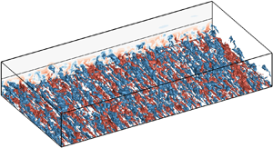
Figure 1. Sketch of the outer–inner interaction between large-scale streamwise rollers (blue circles) and the near-wall low-speed streaks (dashed curves), according to the co-supporting hypothesis in Toh & Itano (Reference Toh and Itano2005). The red and green lines denote the two wall-parallel observation windows, $y=y_{1}$ and $y_{2}$, respectively, used in §§ 3.1 and 3.2.

The choice of the averaging interval $(x_r-\Delta x/2, x_r+\Delta x/2)$ is important. Toh & Itano (Reference Toh and Itano2005), who analysed a streamwise-minimal channel with $L_{x}^{+}=384$, used the full streamwise period $\Delta x=L_x$ as their averaging length. This length is shorter than most streaks, which were thus treated as being infinitely long. Their evolution takes place in time rather than in space, and the same group later showed that the length of the near-wall streaks in a full channel can be substituted by their lifetime in a streamwise-minimal one (Abe, Antonia & Toh Reference Abe, Antonia and Toh2018).

We analyse in this section full-sized channels at substantially higher Reynolds numbers than in either of the two papers above, and some modifications are needed to (3.1)–(3.3). The typical streamwise length of the near-wall streaks, $\ell _{xu}$, is a few thousand wall units (Hoyas & Jiménez Reference Hoyas and Jiménez2006), and averaging over longer segments risks mixing streaks and hiding their spanwise meandering. We use in this paper $\Delta x^+\approx 380$–450, which is short enough to retain structural information, but long enough to differentiate the near-wall streaks from velocity fluctuations of smaller scale. A posteriori tests show that the results below are robust in the range $\Delta x^+ \approx 300$–500.

When $\Delta x=L_x$, the streamwise origin, $x_r$, of the observation box becomes irrelevant, and the near-wall streaks in the streamwise-minimal flow in Toh & Itano (Reference Toh and Itano2005) form branching structures that tend to merge beneath large-scale low-speed regions, supporting their assumed relation between LSMs and the spanwise drift of the streaks. In larger channels, the position of the observation window is crucial. Kim & Hussain (Reference Kim and Hussain1993) and del Álamo & Jiménez (Reference del Álamo and Jiménez2009) showed that the streamwise advection velocity of most quantities in the buffer layer is $u_{ad}^+\approx 10$, and Lozano-Durán & Jiménez (Reference Lozano-Durán and Jiménez2014b) later showed that $u_{ad}^+\approx 8$ for the ejections associated with the low-speed streaks. Farther from the wall, the small scales move approximately with the mean flow velocity, with ejections also moving slightly more slowly than the flow (Lozano-Durán & Jiménez Reference Lozano-Durán and Jiménez2014b). For example, ejections at $y^+=200$ move at $u_{ad}^+=16.7$ while $U(y)^+=18.2$. Centring on the buffer layer, we show that the spanwise drift velocity of the streaks is of the order of $u_\tau$, so that, if the observation window were fixed to the wall, streaks would only be observed over times of the order of $\Delta t^+\approx \ell _{xu}^+/8\approx 100$, during which they would drift at most by $\delta z^+\approx 100$. This is too little to characterise the interactions in which we are interested, which involve VLSMs whose width is $\Delta z\approx h$. Therefore, we track individual streaks by moving the window with their average advection velocity, $x_r=x_{r0} +u_{ad} t$, where $x_{r0}$ is the initial window position.

A typical time history of the spanwise location of low-speed streaks at $y^{+}=5$ is displayed in figure 2(a), using $u_{ad}^+=8$ as representative of the near-wall region. Each line in the figure represents the trajectory of a single low-speed streak, and it is clear from the figure that they substantially drift spanwise. Their mean spanwise spacing, approximately $100$ wall units, agrees well with the known streak spacing near the wall (Smith & Metzler Reference Smith and Metzler1983). Toh & Itano (Reference Toh and Itano2005) classify the trajectories that they observe in streamwise-minimal channels into dominant branches with long lifetimes (of the order of 1000–3000 wall units), and subordinate ones with shorter lifetimes that tend to merge into the dominant ones. The lifetime of such a fragile object as a near-wall streak is hard to define, but Lagrangian scales of 300–1000 temporal wall units were obtained in the buffer layer by Jiménez et al. (Reference Jiménez, Kawahara, Simens, Nagata and Shiba2005), Flores & Jiménez (Reference Flores and Jiménez2010) and Abe et al. (Reference Abe, Antonia and Toh2018). The lifetime of the branches in figure 2(a) is of the same order, 200–800 wall units, and few of them last beyond 1000 viscous time units. They thus correspond to the subordinate branches in Toh & Itano (Reference Toh and Itano2005).

Figure 2. Time history of the spanwise locations of low-speed streaks in a full-sized channel (M950). Locations of the low-speed streaks are determined by the condition (3.1)–(3.3): (a) $y^{+}=5$ and (b) $y^{+}=200$. The red dashed line denotes the averaged location of a large-scale streak.

Figure 2(b) is drawn at $y^{+}=200$, using $u_{ad}^+=16.7$, and represents the logarithmic region. The trajectories cluster in a wide band around $z/h=1.7$, marked by a red dashed line, which appears to be one of perhaps two large streaks that dominate the flow at that level. The interpretation of this figure needs some comment. Although it is known that outer-layer low-speed regions in channels contain more small-scale vortices than high-speed ones (Tanahashi et al. Reference Tanahashi, Kang, Miyamoto, Shiokawa and Miyauchi2004), which could be interpreted as supporting the gathering action hypothesised by Toh & Itano (Reference Toh and Itano2005), the clustering in figure 2(b) is probably an artefact of the detection criterion (3.1). Low-velocity streaks are only recognised as such when they ride on a deeper large streak that lowers their velocity below the mean profile, and what we see in the figure is probably the root of an attached streak centred farther from the wall.

The influence of criterion (3.1) should thus be further discussed. Figure 3 repeats figure 2 without using (3.1). At $y^{+}=5$, condition (3.1) discards part of the scattered dots, which reappear in figure 3, but there are also more coherent streaks in the new figure than in the old one. The spanwise drift of the streaks is present in both figures, but it is evident from comparing them that the streak density measured by (3.1)–(3.2a,b) may be influenced by (3.1). For the result at $y^{+}=200$ in figures 2(b) and 3(b), the condition (3.1) takes a dominant role, and rejects approximately half the local minima. When it is removed, the gathering action suggested by the co-supporting is still observed, although less clearly than before, but it is not reflected in the streak density. Figure 3 shows an almost uniform distribution of small streaks, instead of only the part riding on the larger outer streak. Only condition (3.2a,b) will be used to define the near-wall streaks in the quantitative analysis in the next two sections.

Figure 3. Time history of the spanwise locations of low-speed streaks in a full-sized channel (M950) without the criterion (3.1): (a) $y^{+}=5$ and (b) $y^{+}=200$.

3.1. Spanwise drift of the near-wall streaks versus the outer eddies

Although figures 2 and 3 clearly indicate that the streaks move spanwise, relating their drift to the outer large-scale circulations requires quantitative analysis. The premise of the top-down branch of the co-supporting cycle in Toh & Itano (Reference Toh and Itano2005) is that the near-wall streaks are scattered away from the down-washing regions of the large-scale circulations, and gather in the up-washing ones, as sketched in figure 1. This implies a positive correlation between the spanwise derivative, $\partial v/\partial z$, of the wall-normal velocity of the outer flow and the spanwise drift of the near-wall streaks. A positive spanwise streak velocity near the wall would correspond to a counter-clockwise large-scale circulation, in which $\partial v/\partial z>0$ near the $z$-positions of the roller centres, as depicted by the first and third rolls in figure 1. A negative streak drift velocity would be associated with $\partial v/\partial z<0$.

To quantify how streaks move as a function of their location, $(t,x_r,y_1,z_s)$, we track the evolution of patterns of $u^{(2D)}$, using a method similar to particle-image velocimetry (PIV). Consider a one-dimensional interrogation window, $z_{s}-\Delta \zeta /2< z< z_{s}+\Delta \zeta /2$, which is advected streamwise with the velocity discussed in the previous section. The streak displacement after $\Delta t$ is defined as the position, $\delta z_{max}$, of the maximum of the correlation

(3.4)\begin{align} R_{u^{(2D)}}(\delta z,\Delta t)&=\frac{1}{(I_{0}I_{1})^{{1}/{2}}}\int_{z_{s}-\Delta\zeta/2}^{z_{s}+\Delta\zeta/2}u^{(2D)}(t,x_r,y_1,z)u^{(2D)}(t+\Delta t,x_r\nonumber\\&\quad +u_{ad}\Delta t,y_1,z+\delta z)\,\mathrm{d}z, \end{align}

where $I_{0}$ and $I_{1}$ are, respectively, the mean squares of $u^{(2D)}(t,x_r,y_1,z)$ and $u^{(2D)}(t+\Delta t,x_r+u_{ad}\,\Delta t,y_1,z+\delta z)$, averaged over the same window as in (3.4). In addition, we only accept maxima for which $R_{u^{(2D)}}(\delta z_{max})>0.8$. The spanwise advection velocity is defined as $w_{s}=\delta z_{max}/\Delta t$, and is assigned to the window centre $(x_r, z_s)$. The following discussion focuses on the near-wall streaks at $y_1^+=13$. It uses $\Delta \zeta ^{+}\approx 50$, and an advection velocity of the interrogation window $u_{ad}^+=8$, as in figure 2(a). The results are robust in the range $\Delta \zeta ^{+}\in [30,70]$, and the effect of $\Delta t^+$ and $u_{ad}^+$ is discussed in Appendix A.

The probability density function (p.d.f.) of the drift velocity at different $Re_{\tau }$ shown in figure 4(a) is concentrated approximately in the range $w_s^+=[-2,2]$, independently of the Reynolds number. This is the same order of magnitude as the spanwise velocity fluctuations of the flow, and the two quantities are closely related. The joint p.d.f. of $w_{s}^{+}$ and $w^{+}$ at $y_{1}^{+}=13$ is displayed in figure 4(b) for case M950. It shows a clear correlation between the two variables, providing direct evidence that the drift of the streaks is not due to their internal dynamics, but to the ambient flow.

Figure 4. (a) Probability density function (p.d.f.) of $w_{s}^{+}$ at different $Re_{\tau }$ with $\Delta t^{+}\approx 20$, and $u_{ad}^+=8$: blue solid line, Case W535; black solid line, M950; red solid line, M2000. (b) Joint p.d.f. of the streak spanwise advection velocity, $w_{s}^{+}$, and the spanwise velocity fluctuations, $w^+$ at $y_{1}^{+}=13$. Case M950, and $\Delta t^{+}=20$. The white diagonal is $w^{+}=w_{s}^{+}$.

We next turn our attention to the correlation of the drift velocity with the structures of the outer flow, represented by the wall-normal velocity at $y_2>y_1$, smoothed with a top-hat filter to isolate the large-scale component,

(3.5)\begin{equation} \tilde{v}(x_0,y_2,z_0)=\frac{1}{\Delta z}\intop_{z_{0}-\Delta z/2}^{z_{0}+\Delta z/2} v^{(2D)}(x_0,y_{2},z)\,\mathrm{d}z, \end{equation}

where $v^{(2D)}$ is defined as in (3.3). A typical joint p.d.f. is shown in figure 5. The abscissae are $w_s$ at $y_1^+=13$, and the ordinates are the spanwise derivative of $\tilde {v}$ at $y_2^+=200$. It is evident that the p.d.f. is preferentially aligned to the first and third quadrants, i.e. that a positive spanwise drift of the streaks tends to occur beneath positive $\partial \tilde {v}/\partial z$, and vice versa, in agreement with the top-down model. To verify that the continuous velocity field obtained by the PIV method truly represent the drift of the streaks, the joint p.d.f., using $w_s^+$ collected at the points identified by (3.2a,b) as the streak centres, are also shown by the white contours in figure 5 for comparison. The differences with the PIV results are negligible.

Figure 5. Joint p.d.f. of the spanwise drift velocity $w_{s}^{+}$ at $y_1^+=13$ and $\partial \tilde {v}^{+}/\partial z^{+}$ at $y_2^+=200$: shaded, $w_{s}^{+}$ by PIV; white dashed lines, $w_{s}^{+}$ at the streak centres. Contour levels are $0.1 (0.2) 0.9$ of the maximum probability density. Case M950, $\Delta t^+\approx 20$ and $\Delta z^{+}= 214$.

The mutual dependence of the two quantities can be quantified by the correlation coefficient

(3.6)\begin{equation} R\left(w_s,\dfrac{\partial\tilde{v}}{\partial z}\right)=\dfrac{\sum w_{s}\dfrac{\partial\tilde{v}}{\partial z}} {\left[\sum w_s^2\sum \left(\dfrac{\partial\tilde{v}}{\partial z}\right)^{2}\right]^{{1}/{2}}}. \end{equation}

Appendix A shows that $R(w_s,{\partial \tilde {v}}/{\partial z})$ depends on the PIV parameters, and on the wall-normal positions $y_2$ of the outer-flow. For the case in figure 5, the correlation of the two quantities is $R_{w_s,\partial \tilde {v}/\partial z}\approx 0.2$, but it can be raised to the order of $0.4$ as $y_2$ changes. See Appendix A for the details.

In fact, one of the functions of the window used to define $w_s$ and $\tilde {v}$ is to highlight how the correlation depends on the spanwise wavelength and on the distance from the wall. The top-down correlations considered by Toh & Itano (Reference Toh and Itano2005) and Abe et al. (Reference Abe, Antonia and Toh2018) were restricted to outer scales with $\lambda _{z}\sim h$, but it makes sense to also consider interactions with intermediate scales presenting in the logarithmic layer, for which $100\lesssim \lambda _{z}^{+}$ and $\lambda _{z}\lesssim h$. Consider the inertia tensor of the joint p.d.f. of $w_s$ and the unfiltered $\partial v/\partial z$, defined as

(3.7)\begin{equation} \boldsymbol{I}\left(w_s, \tfrac{\partial v}{\partial z}\right) = \left(\begin{array}{@{}cc@{}} I_{w_{s}w_{s}} & I_{w_{s}(\partial v/\partial z)}\\ I_{({\partial v}/{\partial z})w_{s}} & I_{({\partial v}/{\partial z}) ({\partial v}/{\partial z})} \end{array}\right), \end{equation}

where

(3.8)\begin{equation} I_{ab} =\frac{1}{L_x L_z}\, \iint a(x,z) b(x,z) \,\mathrm{d}z \,\mathrm{d} x. \end{equation}

To isolate the spanwise scale, express each variable as its Fourier transform along $z$, using $\hat {\varphi }(t,x,y,k_{z})$ to represent the Fourier coefficient of $\varphi (t,x,y,z)$ at the spanwise wavenumber $k_{z}$. The different moments can be expressed as integrals over $k_{z}$,

(3.9)\begin{gather} I_{w_{s}w_{s}}=\intop\widehat{w_{s}}\widehat{w_{s}}^{*}\,\mathrm{d}k_{z}, \end{gather}

(3.10)\begin{gather} I_{({\partial v}/{\partial z})({\partial v}/{\partial z})}=\intop {\rm i}k_{z}\hat{v}({\rm i}k_{z}\hat{v})^{*}\,\mathrm{d}k_{z}=\intop k_{z}^{2}(\hat{v}\hat{v}^{*})\,\mathrm{d}k_{z}, \end{gather}

(3.11)\begin{gather} I_{w_{s}({\partial v}/{\partial z})}=I_{({\partial v}/{\partial z})w_{s}}=\intop\mathrm{Re}({\rm i}k_{z}\hat{v}\widehat{w_{s}}^{*})\,\mathrm{d}k_{z}=\intop\mathrm{Re}(\widehat{w_{s}}({\rm i}k_{z}\hat{v})^{*})\,\mathrm{d}k_{z}\nonumber\\ =\intop-k_{z}\mathrm{Im}(\hat{v}\widehat{w_{s}}^{*})\,\mathrm{d}k_{z}, \end{gather}

where the ‘$*$’ superscript denotes complex conjugation, and averaging over $x$ is implied everywhere. A spectral inertia tensor can then be defined for each $k_z$ as

(3.12)\begin{equation} \boldsymbol{I}\left(w_s, \frac{\partial v}{\partial z}; k_z\right) =\left(\begin{array}{@{}cc@{}} \widehat{w_{s}}\widehat{w_{s}}^{*} & -k_{z}\mathrm{Im}(\hat{v}\widehat{w_{s}}^{*})\\ -k_{z}\mathrm{Im}(\hat{v}\widehat{w_{s}}^{*}) & k_{z}^{2}(\hat{v}\hat{v}^{*}) \end{array}\right). \end{equation}

We are interested in the relation of $k_z$ with the height at which $\hat {v}(k_{z})$ has the strongest influence on $w_s$. The strength of this influence can be quantified by the inclination angle $\theta$ of the principal axes of the joint p.d.f. inertia ellipse, and $\theta =\arctan |a_2/a_1|$ can be calculated from the leading eigenvector $(a_{1},a_{2})$ of the inertia tensor. Here we can define a rescaled tensor that avoids derivatives by removing the $k_z$ factors from $\boldsymbol {I}$, for $k_z$ in (3.12) not only bring dimensional complications, but also has a scale-dependent influence on the principal axes:

(3.13)\begin{equation} \boldsymbol{I}\left(w_s, v; k_z\right) =\left(\begin{array}{@{}cc@{}} \widehat{w_{s}}\widehat{w_{s}}^{*} & -\mathrm{Im}(\hat{v}\widehat{w_{s}}^{*})\\ -\mathrm{Im}(\hat{v}\widehat{w_{s}}^{*}) & \hat{v}\hat{v}^{*} \end{array}\right). \end{equation}

This tensor directly relates the velocities at the two wall distances at scale $k_z$, and has the advantage of balancing their magnitudes and dimensions. Note that the imaginary part in the off-diagonal elements of (3.13) has the effect of translating spanwise one of the variables by a quarter wavelength with respect to the other, so that $\boldsymbol {I}(w_s, v; k_z)$ describes the correlation of the streak drift velocity with the shifted wall-normal velocity in the outer flow.

The inclination angle $\theta$ determined by the second and first components of the leading eigenvector of (3.13), with $0<\theta <{\rm \pi} /2$, quantifies the magnitude of the $v$ fluctuations at $y_2$, relative to the drift velocity of the near-wall streaks with which they correlate. The location, $y_2$ of the maximum for each wavelength, $\lambda _z=2{\rm \pi} /k_z$, can be taken to represent the distance from the wall of the centre of the rollers with that spanwise dimension. It is displayed in figure 6, which clearly shows that rollers are most effective at advecting streaks over distances similar to their own height (of the order of $\lambda _z\approx 4y_2$). For example, the maximum correlation in figure 17 in Appendix A is obtained when the wall-normal velocity is smoothed with a filter for which $\Delta z^+\approx 200$ at $y_2^+=100$. As the effect of the eddies responsible for this correlation reaches, by definition, the near-wall region, the self-similar dependence of their size is one more demonstration of the attached-eddy model of Townsend (Reference Townsend1961), and proves that the buffer-layer streaks are not controlled by eddies of a single size, but by the whole hierarchy of attached structures of the logarithmic layer.

Figure 6. Inclination angle, $\theta /{\theta }_{max}$, of the leading eigenvector of the correlation tensor (3.13), as function of $y_{2}$ and of the spanwise wavelength $\lambda _{z}$, where ${\theta }_{max}$ is the maximum of $\theta$ at the corresponding wavelength: (a) W535; (b) M950; (c) M2000.

3.2. Near-wall streak density and the outer region

Having established the influence of the outer structures on the spanwise drift of the streaks of the buffer layer, it remains to be shown whether this drift results in the modulation of the density of streaks. This assumption underlies the second, bottom-up, branch of the co-supporting hypothesis of Toh & Itano (Reference Toh and Itano2005), which proposes that the accumulation of low-speed streaks below an existing outer-flow ejection leads to some kind of collective instability that reinforces the ejection. At first sight, this conclusion is reasonable, because the streaks converge where $\tilde {v}(y_2)>0$ and diverge where $\tilde {v}(y_2)<0$. However, the density of streaks not only depends on their motion, but also on the rate at which they are born and disappear, and it should be clear from the discussion in § 3 that the longest reasonable lifetime of a streak is of the same order as the time required for it to drift across distances of order $h$. In fact, a cursory inspection of figure 3 shows that most streaks do not live long enough to cross spanwise distances of the order of the width of the largest VLSMs, but, because we saw at the end of § 3.1 that streaks also interact with narrower structures closer to the wall, we need to determine whether the same conclusion applies to these structures. In this section we examine directly the correlation of the outer $\tilde {v}$ with the density of buffer-layer streaks.

To quantify this correlation, we again define two spanwise windows, one at $y_1^+=13$ in the buffer layer, and another at $y_2$ in the outer region. Both windows have the same width, $\Delta z$, and are centred at the same wall-parallel location $(x_0, z_0)$, but they serve different purposes. The inner window is used to compute the streak density by counting minima of $u^{(2D)}$, as in (3.2a,b). The outer window is used to compute the smoothed $\tilde {v}$, as in (3.5). The streamwise interval used to compute $u^{(2D)}$ and $v^{(2D)}$ is the same as in § 3, $\Delta x^+=400$, but several $\Delta z$ are used to test their effect on the results. A minimum value for $\Delta z$ can be estimated from physical arguments. As the spacing of the buffer-layer streaks is known to be approximately 100 wall units (Kline et al. Reference Kline, Reynolds, Schraub and Runstadler1967; Smith & Metzler Reference Smith and Metzler1983), and the hypothesis in Toh & Itano (Reference Toh and Itano2005) is that at least two streaks need to merge to generate a larger-scale ‘eruption’, it is reasonable to choose $\Delta z^+\gtrsim 200$. Statistics are compiled by scanning $x_0$, $z_0$ and time. The number of samples in each direction is summarised in table 2. The total number of samples used for each Reynolds number always exceeds $4\times 10^{6}$.

Table 2. Number of samples used for the streak statistics: $n_{x}$, $n_{z}$ and $n_{t}$ denote sample numbers in the $x$, $z$ and $t$ directions, and $N=n_{x} n_{z} n_{t}$ is the total number of samples.

The spanwise density of streaks $\rho _s$ is the inverse of their average spacing, and is simply determined from the number, $n_s$, of minima in the observation window, $\rho _s=n_s/\Delta z$. It follows from the classical estimates of streak spacing that we can expect $\rho _s^+\approx 0.01$.

Distributions of the streak spacing are given in figure 7, compared with the results of Smith & Metzler (Reference Smith and Metzler1983) in a turbulent boundary layer at $Re_{\tau }\approx 724$. Figure 7(a) shows the effect on the spacing of the size of the detection window. As expected, the distribution becomes more concentrated for wider windows, but the mode of the distribution, $\ell _{zu}^{+}\approx 70$, remains constant and is only slightly narrower than the result of Smith & Metzler (Reference Smith and Metzler1983), $\ell _{zu}^{+}\approx 85$. Considering that these authors detect streaks from the accumulation of hydrogen bubbles at $y^+=5$, and determine visually the distance among neighbouring streaks, the discrepancy can probably be attributed to the different definitions of what constitutes a streak. Even so, the p.d.f. obtained with our narrowest window, $\Delta z^+\approx 200$, is fairly close to that in Smith & Metzler (Reference Smith and Metzler1983), and this window is used in the following. Figure 7(b) shows that the density distribution is essentially independent of the Reynolds number, also in agreement with Smith & Metzler (Reference Smith and Metzler1983).

Figure 7. (a) Probability density function of the streak density at different $\Delta z$ in case M2000: black, ${\Delta z}^{+}=214$; red, ${\Delta z}^{+}=308$; blue, ${\Delta z}^{+}=411$; green, ${\Delta z}^{+}=510$; dashed, Smith & Metzler (Reference Smith and Metzler1983). (b) Probability density function of the streak density distributions at different $Re_{\tau }$ and $\Delta z^{+}\approx 200$: blue circles, L550; red circles, M950; black crosses, M2000; green circles, M4200; dashed line, Smith & Metzler (Reference Smith and Metzler1983); full line, the best-fitting curve.

The correlation coefficient between $\rho _{s}$ and $\tilde {v}$ is defined as

(3.14)\begin{equation} R(\rho_{s},\tilde{v})=\frac{\sum(\rho_{s}-\overline{\rho_{s}})\tilde{v}}{\left[\sum(\rho_{s}-\overline{\rho_{s}})^{2}\sum\tilde{v}^{2}\right]^{{1}/{2}}}, \end{equation}

where $\overline {\rho _{s}^{+}}\approx 0.01$ denotes the averaged streak density. The averaged wall-normal velocity vanishes from continuity, and the summation extends over all the samples in table 2. The streak density $\rho _{s}$ is a local quantity depending on the spanwise locations, whereas the correlations between the local $\rho _{s}$ and $\tilde {v}$ could capture the possible streak accumulation. If the streaks really accumulated in the up-washing regions of $\tilde {v}$ and drained away from the down-washing regions, the correlation $R(\rho _{s},\tilde {v})$ would be strongly positive. However, figure 8(a,b) show that the correlation is always smaller than $0.2$, and even turns negative at large $y_2$, contradicting the assumption of the top-down model of Toh & Itano (Reference Toh and Itano2005). This failure can be traced to our rejection of condition (3.1), which was used by Toh & Itano (Reference Toh and Itano2005) when identifying streaks. This criterion has very little influence on the drift statistics in § 3.1, but figure 8(c), as well as figure 3, shows that it strongly affects the results for the streak density. The density is clearly correlated with the outer large-scale circulations when using (3.1), because that condition tends to reject streaks underneath large-scale high-speed regions, and to retain the roots of the low-speed ones. However, when only the local minimum condition (3.2a,b) is used, the accumulation becomes weaker or negative.

Figure 8. (a) Correlation $R(\rho _{s},\tilde {v})$ at different $\Delta z$ in case M2000: black, ${\Delta z}^{+}=214$; red, ${\Delta z}^{+}=308$; blue, ${\Delta z}^{+}=411$; green, ${\Delta z}^{+}=510$. (b) As in (a) for different $Re_{\tau }$ and $\Delta z^{+}\approx 200$: blue, L550; red, M950; black, M2000; green, M4200. (c) Correlation for $\Delta z^{+}=214$ in case M2000: circles, with condition (3.1); crosses, without condition (3.1).

Another effect that may influence the correlation $R(\rho _{s},\tilde {v})$ is the modulation of the local wall shear by the outer LSMs. A negative $\tilde {v}$ brings high-speed fluid from the outer flow towards the wall, increasing the local shear and, in effect, decreasing the local viscous length. If the streak generation process is in equilibrium with this shear, the local streak spacing should decrease and the streak density should increase. This would tend to counteract the hypothesised local decrease in density due to divergence, and decrease the inner–outer correlation. If the modulation is strong enough, it may overcome the correlation completely, and even become negative. The effect is similar to the LSM-induced local wall-shear fluctuations in Abe et al. (Reference Abe, Kawamura and Choi2004) and the large-scale modulations in Mathis et al. (Reference Mathis, Hutchins and Marusic2009), which were also shown in Jiménez (Reference Jiménez2012) and Zhang & Chernyshenko (Reference Zhang and Chernyshenko2016) to be mostly reducible to scaling by the local friction velocity, $(u_\tau )_{local}=(\nu \, \partial \tilde {u}/\partial y)^{{1}/{2}}$.

Figure 9 shows that the effect is not trivial, and confirms that it is a consequence of the interaction with the outer flow. Figure 9(a) presents the p.d.f. of $(u_\tau )_{local}$ for three Reynolds numbers, computed over a spanwise averaging window whose size scales in wall units. The variation is of the order of $\pm 20\,\%$, and widens as the Reynolds number increases, in agreement with the increase in energy from the wider range of scales of the velocity fluctuations. If the effect were local to the near-wall layer, it would be difficult to explain this Reynolds number dependence. In fact, figure 9(b) shows that, when the averaging window is scaled in outer units, the variation of $(u_\tau )_{local}$ depends on the size of the window, but not on the Reynolds number.

Figure 9. Probability density function of $(u_\tau )_{local}/u_\tau$ at different $Re_{\tau }$, where $(u_\tau )_{local}$ is the local friction velocity computed over each window, and $u_\tau$ is its global average: (a) ${\Delta z}^{+}\approx 200$; blue solid line, L550; red solid line, M950; black solid line, M2000; (b) ${\Delta z}/h\approx 0.4$; blue solid line, L550; red dashed line, M950; ${\Delta z}/h\approx 0.2$, red solid line, M950; black dashed line, M2000.

Finally, figure 10 shows that, when both $\rho _{s}^{+}$ and $\tilde {v}^{+}$ are scaled in the local wall units, the effect of the averaging window on $R(\rho _{s}^{+},\tilde {v}^{+})$ largely disappears, but the correlation still decays with $y_2$. It becomes negligible above $y_2^+\approx 150$ but, in contrast to figures 8(a) and 8(b), it does not become negative at higher $y_2$. It is interesting that the limit for this decay scales in wall units, suggesting that the reason has more to do with the dynamics of the buffer layer than with the outer flow.

Figure 10. Correlation $R(\rho _{s}^{+},\tilde {v}^{+})$ scaled in local wall units. (a) At different window size in case M2000: black, ${\Delta z}^{+}\approx 214$; red, ${\Delta z}^{+}\approx 308$; blue, ${\Delta z}^{+}\approx 411$; green, ${\Delta z}^{+}\approx 510$. (b) At different $Re_{\tau }$ when $\Delta z^{+}\approx 200$: blue, L550; red, M950; black, M2000; green, M4200.

What needs to be explained is why streaks drift spanwise but do not accumulate, and the simplest explanation is their short lifetime, which is $t^{+}=O(500)$ instead of the $t^{+}=1000\text {--}3000$ in Toh & Itano (Reference Toh and Itano2005). As $w_s^+=O(1)$, their maximum drift is thus only $\delta z^+ =300\text {--}500$ (see figure 3a), and the outer structures can only couple with the streak density over widths of this order. It follows from figure 6 that this corresponds to $y_2^+\approx 100$, and that the accumulation hypothesised in Toh & Itano (Reference Toh and Itano2005) is a wall-layer effect that should become increasingly less relevant as the Reynolds number increases.

4. Bottom-up influence on the LSM generation and preservation

In order to examine the possibility of bottom-up influence during the LSM generation process, two further numerical experiments are performed. In the first, the flow in the channel is initialised with a laminar velocity profile near the upper wall and a turbulent velocity profile near the lower wall, as in Schoppa & Hussain (Reference Schoppa and Hussain2002). The initial perturbations, added below $y^{+}=50$ in the lower half of the channel, are constructed by filtering the flow in case W535 to retain the velocity fluctuations with $\lambda _{z}^{+}<230$. As experience shows that early flow adjustments kill part of these perturbations, they are amplified by a moderate factor (approximately 1.3) before being added to the flow, so that the near-wall Reynolds stress is similar to the fully developed one after the initial decay. This ensures that the channel transitions to turbulence, and is robust to amplification factors up to two. Part of the adjustment is the imposition of continuity by the first simulation step, which is not initially satisfied near the upper boundary of the added streaks $(y^{+}=50)$, but the effect is minor. The code and computational parameters are as in W535 (see table 1), with the Reynolds number fixed to $Re=U_{m}h/\nu =9800$, which corresponds to $Re_{\tau }\approx 535$ near the lower wall.

Before detailed quantitative analysis, it is helpful to have an overview of the development of the flow. Figure 11 shows the time history of the local $Re_{\tau }$ on the upper and lower walls. The lower-wall $Re_{\tau }$ initially decreases a bit, and then increases until $t=20$, gradually approaching its target value of $Re_{\tau }=535$. On the upper wall, the flow remains laminar until turbulent transition occurs around $t=60$. The upper $Re_{\tau }$ then quickly increases until $t=75$, after which it approaches its turbulent level, $Re_{\tau }=535$. The time evolution of the mean velocity profile is displayed in figure 12, non-dimensionalised by the local wall units at the corresponding time instants. In the lower side, shown in figure 12(a), the profile overlaps the fully developed one below $y^{+}=20$ for $t=10\text {--}50$, and the agreement gradually extends to higher positions as time develops. This suggests that turbulent structures are gradually being constructed at higher positions as the flow approaches equilibrium. After $t=50$, the mean velocity profile collapses to the fully developed flow. In the upper half-channel, shown in figure 12(b), the profile quickly changes from laminar to turbulent as that wall transitions at $t=60\text {--}70$, as also indicated by the abrupt increase of $Re_{\tau }$ in figure 11. The flow continues to adjusts after $t=80$, and the whole channel then evolves to a fully developed turbulent state.

Figure 11. Time history of the local $Re_{\tau }$ on the upper (blue solid line) and lower (red solid line) walls. The dashed vertical lines (1)–(6) mark the corresponding time instants in figures 13 and 18: (1) $t=5$, (2) $t=20$, (3) $t=30$, (4) $t=50$, (5) $t=60$ and (6) $t=68$.

Figure 12. Time evolution of the mean velocity profile, $U^{+}$, scaled in local wall units. (a) In the lower half-channel from $t=10$ to $t=50$: red solid line, $t=10$; pink solid line, $t=20$; green solid line, $t=30$; sky blue solid line, $t=40$; blue solid line, $t=50$. And (b) in the upper half-channel, from $t=50$ to $t=90$: red dashed line, $t=50$; pink dashed line, $t=60$; green dashed line, $t=70$; sky blue dashed line, $t=80$; blue dashed line, $t=90$. The black lines (black solid line) denote the profile in case W535. The arrows indicate increasing time.

Figure 13. Distributions of $u^{\prime }$ in the lower half-channel at (a) $t=5$, (b) $t=20$ and (c) $t=30$. Length in the $x$ direction is ${2{\rm \pi} }$ and in the $z$ direction is $4{\rm \pi}$. Red: ${u^{\prime }}^{+}=3$; blue: ${u^{\prime }}^{+}=-3$. Flow is from bottom right to top left.

We consider in this section the evolution of the flow structures near the lower wall, where the initial perturbations are added. The evolution of the upper half-channel is closer to classical bypass transition, and is discussed in Appendix B. The distribution of the streamwise velocity fluctuations in the lower half-channel is displayed in figure 13 at the three selected times indicated by the lines (1)–(3) in figure 11. At $t=5$, the perturbations are confined to the near-wall region, which is dominated by small-scale velocity streaks. Turbulent fluctuations gradually spread farther from the wall, in accordance with the evolution of the velocity profile in figure 12, and streaks of increasingly larger scales appear at $t=20$ and $30$. The approximate size of the largest streaks at $t=20$ is $\lambda _{z}\sim 0.7h$, and they grow to $\lambda _{z}\sim h$ at $t=30$. The turbulent fluctuations visually occupy the whole lower half-channel after that time.

The evolution of the streamwise velocity fluctuations towards larger scales can be quantified by the time-dependent spanwise energy spectrum, defined as

(4.1)\begin{equation} E_{uu}(t,y,k_{z})=\frac{1}{L_{x}}\intop_{0}^{L_{x}} (\left|\hat{u}(t,x,y,k_{z})\right|^{2}+\left|\hat{u}(t,x,y,-k_{z})\right|^{2})\,\mathrm{d} x. \end{equation}

The evolution of its integral over the lower half-channel, $E_{uu}^{\forall }(t,\lambda _{z})$, is shown in figure 14 as a function of $\lambda _{z}$ and of time. The energy is initially concentrated around $100<\lambda _{z}^{+}<230$, where the initial perturbations have been introduced, and spreads to wider wavelengths as LSMs are gradually generated. The final peak at $\lambda _{z}\sim h$ develops for $t\gtrsim 30$, in accordance with figure 13. The numerical experiment evolves to a fully developed turbulent state after $t=120$, with much lower fluctuations compared with the peaks before $t=100$.

Figure 14. Time evolution of ${k}_{z}E_{uu}^{\forall }(t,\lambda _{z})$ as a function of $\lambda _{z}$ in the lower half-channel. The vertical white lines mark the time instants $t=5$, $20$ and $30$.

After confirming that the flow is able to generate LSMs with the only input of initially imposed near-wall streaks, the question of whether streak accumulation is required for this generation is explored by means of the temporal evolution of the correlation (3.14) between the near-wall streak density, $\rho _{s}(y_1^+=13)$, and the wall-normal velocity $\tilde {v}(y_2)$. Figure 15(a) presents the time history of this correlation coefficient $R(t, y_2)$, with an averaging window $\Delta z^{+}\approx 200$.

Figure 15. (a) Time history of the correlation $R(\rho _{s},\tilde {v})$ with $\Delta z^{+}\approx 200$. Vertical white lines mark the time instants $t=5$, $20$ and $30$. (b) The correlation $R$ between $\tilde {v}(x,y_{2},z,t_{0})$ and $\rho _{s}(x-x_{ad},y_{1},z,t_{0}-\Delta t)$ as function of $\Delta t$. Here $\Delta z^{+}\approx 200$. The statistics are compiled by scanning $x$ and $z$; $t_{0}=30h/U_{m}$ and $x_{ad}=(u_{ad}(y_{2})-u_{ad}(y_{1}))\Delta t$ is the streamwise offset due to the different advection velocities.

The wall-normal locations for which $R>0.1$ are confined below $y_2^+=100$, implying only local interactions within the buffer layer, and no change can be observed before or after the LSMs appear at $t \approx 30$. Therefore, the conclusion reached in § 3.2 approximately the lack of correlation between the streak density and the outer velocity also applies to the LSM generation process.

The same lack of correlation holds when a delay is introduced in $R$. The correlation between $\tilde {v}(y_2, t_0)$ and $\rho _{s}(y_1,t_{0}-\Delta t)$ is shown in figure 15(b) as a function of $\Delta t$. If the outer LSMs were a result of streak accumulation, as assumed by the bottom-up hypothesis, this correlation should peak at some finite delay, but it is clear from the figure that the correlation maximum is at $\Delta t=0$, and that it never reaches above $y^+_2\approx 30$. This again argues against the hypothesis that the formation of outer scales is due to the previous accumulation of streaks in the near-wall region.

Although this numerical experiment shows that the generation of LSMs does not depend on the accumulation of the near-wall streaks, it could still be possible that the maintenance of the LSMs depends on the existence of large-scale non-uniformities near the wall. This is tested by a second numerical experiment, in which the LSMs below $y^{+}=50$ are artificially removed after the flow has become fully turbulent in the first experiment.

Fourier filtering is applied at $t=300$ to the lower side of the channel below $y^{+}=50$, to remove the fluctuations of the three velocity components with $\lambda _{z}>h/2$. The subsequent evolution of the streamwise turbulent kinetic energy at scales $\lambda _{z}>h$ is displayed in figure 16(a). The influence of the filtering gradually rises to $y^{+}\approx 100$, whereas new energy appears in the buffer layer at $t\approx 305$, with a local maximum near $t=308$, possibly reflecting the top-down influence of the LSMs remaining in the outer region. The adjustment of the buffer layer lasts until $t\thickapprox 315$, after which $E_{uu}$ recovers its equilibrium distribution. The time evolution of $k_{z}E_{uu}$ at $y^{+}=200$ during this recovery process is displayed in figure 16(b). The energy peak at $\lambda _{z}\approx 1.5h$ evolves smoothly with time, and the influence of the disturbed buffer layer can hardly be seen.

Figure 16. Time evolution of (a) $\sum _{\lambda _{z}>h}k_{z}E_{uu}(t,y^{+},\lambda _{z})$ and (b) $k_{z}E_{uu}$ at $y^{+}=200$ in the lower half-channel from $t=285$ to $t=330$. The vertical white lines are $t=300$ and $t=315$.

This result suggests that the removal of LSMs below $y^{+}=50$ has little impact on the preservation of LSMs in the outer region. Notably, the adjustment time of the buffer layer in response to the sudden filtering is approximately ${\Delta t}=15h/U_{m}$ ($\Delta t^{+}\thickapprox 440$), which is of the same order as the average lifetime of LSMs at the present Reynolds number (Lozano-Durán & Jiménez Reference Lozano-Durán and Jiménez2014b), and should thus be long enough for the LSMs to decay if their maintenance mechanism had been interrupted. Figure 16(b) shows that they do not.

In summary, the twin experiments in this section strongly suggest that the production and preservation of LSMs in the outer region do not rely on the existence of large-scale organisation in the near-wall region, in accordance with the results of Flores & Jiménez (Reference Flores and Jiménez2006) and others mentioned in the introduction. They all suggest that the possible bottom-up influence is not essential for the preservation of the outer structures.

5. Summary and conclusions

The inner–outer co-supporting model of Toh & Itano (Reference Toh and Itano2005), which had up to now only been studied in turbulent channels with short simulation boxes, has been examined in full-sized simulations at low to moderate Reynolds numbers. The model has three stages: the near-wall streaks drift in the spanwise direction under the influence of the outer LSMs; they accumulate in areas of large-scale velocity convergence; and areas of high streak density lead to the formation of new LSMs.

We have confirmed the first stage by tracking near-wall streaks by a method similar to PIV. The streaks drift spanwise with velocities of the order of $\pm u_\tau$, and this drift is correlated with the large-scale velocity of the outer structures. Moreover, the coupling not only happens between the wall and the largest LSMs. Structures centred at distance $y$ from the wall in the logarithmic layer couple most strongly with the drift of streaks over spanwise distances of $O(y)$, in agreement with the standard model of a hierarchy of wall-attached eddies (Townsend Reference Townsend1961).

The evidence for streak accumulation is less clear, and we have shown that most of the effect observed in Toh & Itano (Reference Toh and Itano2005) and Abe et al. (Reference Abe, Antonia and Toh2018) is due to their requirement that streaks should have a streamwise velocity lower than the mean profile. When this condition is removed, the streak density becomes fairly uniform, and its correlation with the outer structures mostly disappears. In fact, it even changes sign far enough from the wall. The latter also turns out to be due to the spurious modulating effect of the non-uniform wall shear induced by the large outer scales. When this is taken into account, the correlation between the outer flow and the streak density is uniformly positive, but mostly restricted to structures below $y^+\approx 150$, suggesting that the co-supporting cycle is a wall-layer effect that becomes less relevant as the Reynolds number increases. The reason is traced to the lifetime of the streaks, which is too short to couple to higher and wider structures, but which is probably artificially stabilised by the short simulation boxes in Toh & Itano (Reference Toh and Itano2005) (interestingly, this possibility was anticipated in that paper, but largely forgotten afterwards).

In addition to the examination and quantification of the top-down influence, the bottom-up branch of the cycle is investigated by means of two numerical experiments that facilitate the artificial isolation of the structures at different scales. The first focuses on the generation process of LSMs, starting from artificially assembled near-wall streaks in an otherwise fluctuation-less flow. The correlation between the streak density and the outer flow changes little before or after the LSM spontaneously appear and their size gradually grows. Moreover, the streak accumulation history hardly influences the appearance of large-scale components of the wall-normal velocity, implying that the streak merging does not have a strong relation with the generation of the LSMs.

A final experiment concentrates on the preservation of existing LSMs. The large-scale component of the velocity fluctuations in the near-wall region is filtered out once the flow is fully established, but the outer LSMs are essentially unaffected during the regeneration of the buffer region. Both experiments argue against the bottom-up branch of the co-supporting hypothesis of Toh & Itano (Reference Toh and Itano2005).