


1 Introduction
The flight of flapping-wing micro air vehicles (FWMAVs) is relatively costly compared to that of large gliders due to the increased viscous resistance at small scales. However, the high lift generated as a result of multiple unsteady mechanisms, such as the delayed stall and the clap-and-fling mechanisms, makes flapping essential for a stable flight at low Reynolds numbers (Sane Reference Sane2003). The flapping-wing mechanism in FWMAVs has been inspired by that of insects. A flapping stroke comprises the rotational translation (or sweep) during a half-stroke, followed by the flip motion (or pitch) towards the end of the half-stroke. Two such half-strokes, namely the upstroke and downstroke, make a single flapping stroke. The mean lift force generated as a result of various unsteady mechanisms depends on the flapping-motion pattern of the wing, which also affects the flight economy. Hence, in order to have a complete understanding of the kinematic efficiency of a flyer, it is important to study its flapping kinematics.
An insect wing is free to rotate around three orthogonal axes, allowing three degrees of freedom. The corresponding three Euler angles represent the phase angle ( $\unicode[STIX]{x1D719}$), the pitch angle (
 $\unicode[STIX]{x1D713}$) and the deviation angle (
 $\unicode[STIX]{x1D703}$). It has been established that during ‘normal hovering’, an insect wing is minimally deviated (i.e.
  $\unicode[STIX]{x1D703}\sim 0$) and the wing flaps symmetrically in upstroke and downstroke along nearly a single horizontal plane (Rayner Reference Rayner1979; Maxworthy Reference Maxworthy1981). Hence, the important angles in this mode are
  $\unicode[STIX]{x1D719}$ and
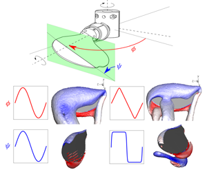
  $\unicode[STIX]{x1D6FC}$, which are shown in the schematic in figure 1. Following the convention from the literature (e.g. Chen & Skote Reference Chen and Skote2016), the angle of attack (
 $\unicode[STIX]{x1D6FC}$) is related to the pitch angle as
  $\unicode[STIX]{x1D6FC}=\unicode[STIX]{x03C0}/2-|\unicode[STIX]{x1D713}|$. It should be noted that the forces on an insect-style flapping wing are stabilised by the stable attachment of the leading-edge vortex (LEV) (see Ellington et al. Reference Ellington, van den Berg, Willmott and Thomas1996). The LEV is a peculiar feature of a rotating wing, which is stabilised on account of the strong spanwise flow driven by the Coriolis and centripetal accelerations (Lentink & Dickinson Reference Lentink and Dickinson2009), unlike its periodic shedding in the wake of a two-dimensional (2-D) heaving and pitching wing. Hence, a study of three-dimensional (3-D) flapping kinematics is different from that of 2-D kinematics and needs to be explored further.
Previous optimisation studies of wing kinematics can be broadly divided into three groups. The first group involves studies (e.g. Izraelevitz & Triantafyllou Reference Izraelevitz and Triantafyllou2014; Van Buren et al. Reference Van Buren, Floryan, Quinn and Smits2017) investigating the optimal waveforms of heaving and pitching of 2-D wings. The second group includes a number of studies (e.g. Altshuler et al. Reference Altshuler, Dickson, Vance, Roberts and Dickinson2005; Ansari, Knowles & Zbikowski Reference Ansari, Knowles and Zbikowski2008; Young, Lai & Germain Reference Young, Lai and Germain2008; Khan & Agrawal Reference Khan and Agrawal2011) investigating the optimised parameters, such as wing-sweep amplitude ( $\unicode[STIX]{x1D719}_{A}$), pitch amplitude (
 $\unicode[STIX]{x1D713}_{A}$), flapping frequency (
 $f$) and phase of flip rotation
  $(\unicode[STIX]{x1D6FF}_{\unicode[STIX]{x1D713}})$, in 3-D flapping. The third group involves studies (e.g. Sane & Dickinson Reference Sane and Dickinson2001; Berman & Wang Reference Berman and Wang2007; Ghommem et al. Reference Ghommem, Hajj, Mook, Stanford, Beran and Watson2013; Zheng, Hedrick & Mittal Reference Zheng, Hedrick and Mittal2013; Nakata, Liu & Bomphrey Reference Nakata, Liu and Bomphrey2015) investigating optimal 3-D flapping-motion waveforms. Studies from the first group have been primarily inspired by fish-like propulsion. However, the mechanism involved in the force generation on small-aspect-ratio 3-D flapping wings of insects is different (Garmann & Visbal Reference Garmann and Visbal2013). Studies from the second group have investigated optimised parameters with either a harmonic or a robofly-like trapezoidal waveform (similar to that used by Dickinson and co-workers). However, the flapping-motion waveforms of real insects have been observed to correspond to neither of those (see Ellington Reference Ellington1984; Fry, Sayaman & Dickinson Reference Fry, Sayaman and Dickinson2005). Finally, studies from the third group have investigated the effects of pitch duration and timing, which indeed determine the pitch waveform, but show contradictory results as discussed later in this section. However, the sweep waveform, which strongly influences the instantaneous lift coefficient and is a key factor of this paper, has not been varied in any of these studies, except in that by Berman & Wang (Reference Berman and Wang2007). In fact, the optimisation study by Berman & Wang (Reference Berman and Wang2007) is based on the quasi-steady model for force predictions, which does not involve the understanding of the flow physics responsible for the resulting optimised waveforms. Therefore, to our best knowledge, the systematic study of the individual and combined effects of both the sweep and pitch waveforms of an insect-like flapping wing has remained under-explored.

Figure 1. The schematics show (a) the flapping-wing set-up and (b) the alignment of the forces measured using an ATI-Nano17 F/T transducer attached to the wing root. The coordinates are shown in the wing’s reference frame, where the  $Y$ axis is aligned with the sweep axis and the
  $Z$ axis is aligned with the pitch axis along the wingspan.
Bos et al. (Reference Bos, Lentink, Van Oudheusden and Bijl2008) have compared the harmonic, robofly and real fruit-fly waveform models using a 2-D flapping wing and have shown that the real fruit-fly model results in maximum lift coefficient and lift-to-drag ratio. Interestingly, Berman & Wang (Reference Berman and Wang2007) have suggested the following parametric model to systematically vary both the sweep- and pitch-motion waveforms from harmonic to robofly-style motion:
 $$\begin{eqnarray}\left.\begin{array}{@{}c@{}}\displaystyle \unicode[STIX]{x1D719}(t)=\frac{\unicode[STIX]{x1D719}_{A}}{\sin ^{-1}K}\sin ^{-1}[K\sin (2\unicode[STIX]{x03C0}ft+\unicode[STIX]{x1D6FF}_{\unicode[STIX]{x1D713}})]\quad \text{and}\\ \displaystyle \unicode[STIX]{x1D713}(t)=\frac{\unicode[STIX]{x1D713}_{A}}{\tanh (C_{\unicode[STIX]{x1D713}})}\tanh [C_{\unicode[STIX]{x1D713}}\sin (2\unicode[STIX]{x03C0}ft)],\end{array}\right\}\end{eqnarray}$$
 where  $K$ is the sweep profile parameter,
  $C_{\unicode[STIX]{x1D713}}$ is the pitch profile parameter and
  $\unicode[STIX]{x1D6FF}_{\unicode[STIX]{x1D713}}$ is the pitching phase offset. Berman & Wang (Reference Berman and Wang2007) have varied
  $K$ from 0, for the sinusoidal waveform, to 1, for the robofly-like sweep waveform. For the pitch motion, they have varied
  $C_{\unicode[STIX]{x1D713}}$ from 0, for the sinusoidal waveform, to 10, for the robofly-like pitch waveform. Their optimisation study has shown that, for a lift just sufficient to support the insect mass, high
  $K$ (
$K$ ( ${>}0.7$) and low
  $C_{\unicode[STIX]{x1D713}}$ (
 ${<}2.5$) are desirable to achieve low flapping-power consumption. However, their optimisation study uses the forces and torques predicted using quasi-steady models, which do not explain the flow physics behind the minimum power consumption with the optimised parameters. Moreover, their force prediction model uses the lift and drag coefficients reported by Dickinson, Lehmann & Sane (Reference Dickinson, Lehmann and Sane1999), which have been obtained using only the robofly model. These coefficients differ strongly from those for other motion waveforms, as observed in the present study.
A computational study of pitch waveforms of a 2-D wing by Bluman & Kang (Reference Bluman and Kang2017) has shown results contradictory to those of Berman & Wang (Reference Berman and Wang2007). Bluman & Kang (Reference Bluman and Kang2017) have investigated the stability of the flapping system and showed that slow pitching, i.e. a low  $C_{\unicode[STIX]{x1D713}}$, makes the system more unstable than one with rapid pitching. Moreover, previous experiments by Sane & Dickinson (Reference Sane and Dickinson2001) of a 3-D flapping wing have predicted a high lift coefficient and lift/drag ratio with rapid pitching, suggesting that a high
  $C_{\unicode[STIX]{x1D713}}$ is desirable. Other 2-D computational studies (e.g. Khan & Agrawal Reference Khan and Agrawal2011; Ghommem et al. Reference Ghommem, Hajj, Mook, Stanford, Beran and Watson2013) have also varied the duration of pitch in a flapping cycle and showed that a slow pitching, i.e. a low
  $C_{\unicode[STIX]{x1D713}}$, is necessary for a minimum power consumption. However, their 2-D model of a flapping wing comprises linear translation and pitching. The LEV, as mentioned earlier, cannot be observed to be stable in a 2-D flapping-motion model. Hence, a change in the additional lift generated by the rotational accelerations, with a change in the sweep waveform, cannot be predicted well by 2-D models. In short, to achieve the best possible performance of a FWMAV, it is important to identify the optimal flapping waveforms for both the sweep and pitch motions. It is also necessary to observe the relation between the complex 3-D flow structure over the wing and the aerodynamic forces, which can reveal the influence of flapping waveforms on the flow instabilities.
In the present experimental study motivated by insect-scaled MAVs, a fruit-fly wing planform is made to flap at a span-based Reynolds number of  $Re_{b}=215$ using various motion waveforms for
  $\unicode[STIX]{x1D719}$ and
  $\unicode[STIX]{x1D713}$. The performance is computed from the direct measurements of forces and torques along the three Cartesian axes. The cycle-averaged lift and power economy, derived from the measurements, are observed to vary with changes in the values of
  $K$ and
  $C_{\unicode[STIX]{x1D713}}$. Computational simulations of the chosen flapping-wing cases reveal the detailed variations in flow structures with
  $K$ and
  $C_{\unicode[STIX]{x1D713}}$. Additionally, a comparison of a real fruit-fly-style flapping motion with the simplified parametric flapping model indicates that the flapping motion in nature is reasonably optimised for minimum power. The parametric model allows the optimisation of
  $K$ and
  $C_{\unicode[STIX]{x1D713}}$ values to achieve higher lifts. The lift coefficient and power economy mapped on the plane of
  $K$ and
  $C_{\unicode[STIX]{x1D713}}$ can help designers in selecting the optimum flapping-motion profile based on the desired output for their MAVs.
2 Method
This study was conducted using a wing flapping at a fixed Reynolds number, with varying flapping-motion waveforms. As mentioned earlier, the study was motivated by developments in insect-scaled MAVs. In this regard, fruit-fly wing kinematics has been widely explored in the past. Fruit flies are observed to flap their wings at Reynolds numbers in the range [120–170] based on the wing chord and the wing-tip velocity (Fry et al. Reference Fry, Sayaman and Dickinson2005). This range is scaled to, approximately, [200–280], based on the wingspan ( $b$) and the mean velocity at the radius of gyration (
 $R_{g}$). This span-based scaling of the Reynolds number (
 $Re_{b}$) has been shown to appropriately govern the large-scale flow structures over a wing in our recent studies (Harbig, Sheridan & Thompson Reference Harbig, Sheridan and Thompson2013; Bhat et al. Reference Bhat, Zhao, Sheridan, Hourigan and Thompson2019). In the case of flapping wings,
  $Re_{b}$ is defined as
 $$\begin{eqnarray}Re_{b}=\frac{\overline{U}_{g}b}{\unicode[STIX]{x1D708}},\end{eqnarray}$$
 where  $\overline{U}_{g}$ is the cycle-mean velocity at
  $R_{g}$ given by
  $\overline{U}_{g}=4n\unicode[STIX]{x1D719}_{A}R_{g}$,
  $n$ is the flapping frequency,
  $\unicode[STIX]{x1D719}_{A}$ is the stroke amplitude and
  $\unicode[STIX]{x1D708}$ is the kinematic viscosity of the medium. Throughout this study, the stroke amplitude and the frequency were maintained to be constant (
 $\unicode[STIX]{x1D719}_{A}=70^{\circ }$ and
  $n=0.55~\text{Hz}$), such that
  $Re_{b}=215$, which was within the fruit-fly range. The mean force and energy calculations for a wide range of flapping-motion waveforms were obtained from the direct experimental measurements. The detailed variations in vortical structures over the wing with the changes in the waveforms were obtained using 3-D computational simulations.
2.1 Flapping-wing experiments
The experiments were performed on a fruit-fly (Drosophila melanogaster) wing planform of wingspan  $b=0.12~\text{m}$ and aspect ratio
 ![]() , fabricated from a stiff 2 mm thick acrylic sheet. The wing was attached rigidly to an ATI-Nano17 IP68 transducer. The transducer could measure forces with an accuracy of 0.003 N and torques with an accuracy of 0.015 N mm. The transducer, along with the wing, was attached to a flapping mechanism allowing motion of two degrees of freedom. The flapping mechanism was driven using two servo motors (EC-max30, Maxon Motor). Motor-1 controlled the sweep motion via the main shaft. Motor-2 controlled the pitch motion via a timing belt-and-pulley mechanism placed inside the hollow main shaft. The parts of the flapping-wing assembly are shown in an exploded view in figure 2(a). The transducer and the attachments caused the wing to be offset from the sweep axis such that the offset ratio was
, fabricated from a stiff 2 mm thick acrylic sheet. The wing was attached rigidly to an ATI-Nano17 IP68 transducer. The transducer could measure forces with an accuracy of 0.003 N and torques with an accuracy of 0.015 N mm. The transducer, along with the wing, was attached to a flapping mechanism allowing motion of two degrees of freedom. The flapping mechanism was driven using two servo motors (EC-max30, Maxon Motor). Motor-1 controlled the sweep motion via the main shaft. Motor-2 controlled the pitch motion via a timing belt-and-pulley mechanism placed inside the hollow main shaft. The parts of the flapping-wing assembly are shown in an exploded view in figure 2(a). The transducer and the attachments caused the wing to be offset from the sweep axis such that the offset ratio was  $b_{0}/b=0.5$. From a previous study, for this offset ratio, the forces over the wing can be assumed to be minimally affected by the central body (Bhat et al. Reference Bhat, Zhao, Sheridan, Hourigan and Thompson2019). Other parameters, which were maintained to be constant, are the pitch amplitude (
 $\unicode[STIX]{x1D713}_{A}=45^{\circ }$) and the pitching phase offset (
 $\unicode[STIX]{x1D6FF}_{\unicode[STIX]{x1D713}}=90^{\circ }$).

Figure 2. (a) The parts of the flapping-wing rig assembly are shown in an exploded view. (b) A photograph of the assembled set-up of the flapping-motion rig.
As shown in the photograph in figure 2(b), the flapping-motion rig was mounted on a square tank of size  $0.5\times 0.5\times 0.6~\text{m}^{3}$ filled with Stella food-grade mineral oil of kinematic viscosity
  $\unicode[STIX]{x1D708}\sim 150~\text{mm}^{2}~\text{s}^{-1}$. This high viscosity helped to maintain sufficiently high signal-to-noise ratio of the force measurements, even at low Reynolds number. Mineral oil also helped to reduce the noise levels in the recorded signals by electrically and thermally isolating the transducer. The kinematic viscosity was found to vary with ambient temperature. Accordingly, the flapping frequency was adjusted before each experimental run such that
  $Re_{b}$ remained constant.
The ATI-Nano17 transducer was attached to the wing in such a way that it always measured the forces and torques along the axes fixed to the wing’s reference frame. As can be seen in figure 1(b), the transducer measured the forces along the wing chord ( $F_{c}$) and normal to the wing (
 $F_{n}$). The lift and drag over the wing were calculated as
 $$\begin{eqnarray}L=F_{c}\cos (\unicode[STIX]{x1D713})+F_{n}\sin (\unicode[STIX]{x1D713})\quad \text{and}\quad D=-F_{c}\sin (\unicode[STIX]{x1D713})+F_{n}\cos (\unicode[STIX]{x1D713}),\end{eqnarray}$$
respectively. The lift and drag coefficients of the wing were computed as
 $$\begin{eqnarray}C_{L}=\frac{2L}{\unicode[STIX]{x1D70C}\overline{U}_{g}^{2}S}\quad \text{and}\quad C_{D}=\frac{2D}{\unicode[STIX]{x1D70C}\overline{U}_{g}^{2}S},\end{eqnarray}$$
 where  $\unicode[STIX]{x1D70C}$ is the density of the mineral oil and
  $S$ is the wing area. The transducer also measured the torques about the axes along the chord and the normal, referred to as
  $\unicode[STIX]{x1D70F}_{c}$ and
  $\unicode[STIX]{x1D70F}_{n}$, respectively. Hence, the torques along the
  $X$ axis and
  $Y$ axis were computed as
 $$\begin{eqnarray}\unicode[STIX]{x1D70F}_{x}=-\unicode[STIX]{x1D70F}_{c}\sin (\unicode[STIX]{x1D713})+\unicode[STIX]{x1D70F}_{n}\cos (\unicode[STIX]{x1D713})+b_{ati}\times L\quad \text{and}\quad \unicode[STIX]{x1D70F}_{y}=\unicode[STIX]{x1D70F}_{c}\cos (\unicode[STIX]{x1D713})+\unicode[STIX]{x1D70F}_{n}\sin (\unicode[STIX]{x1D713})+b_{ati}\times D,\end{eqnarray}$$
 respectively. Note that the terms  $b_{ati}\times L$ and
  $b_{ati}\times D$ are added since the tool side of the ATI transducer is situated away from the origin by an offset
  $b_{ati}=48~\text{mm}$. The calculated moment coefficients, using this correction, show a close match with those from computational predictions, as shown in appendix A. Moreover, the force and torque measured along the wingspan (
 $Z$ axis) were referred to as
  $F_{z}$ and
  $\unicode[STIX]{x1D70F}_{z}$, respectively. The coefficients of moments along the
  $X$,
$X$,  $Y$ and
  $Z$ axes were computed as
 $$\begin{eqnarray}C_{m_{x}}=\frac{2\unicode[STIX]{x1D70F}_{x}}{\unicode[STIX]{x1D70C}\overline{U}_{g}^{2}Sb},\quad C_{m_{y}}=\frac{2\unicode[STIX]{x1D70F}_{y}}{\unicode[STIX]{x1D70C}\overline{U}_{g}^{2}Sb}\quad \text{and}\quad C_{m_{z}}=\frac{2\unicode[STIX]{x1D70F}_{z}}{\unicode[STIX]{x1D70C}\overline{U}_{g}^{2}Sb}.\end{eqnarray}$$
 The motors driving the flapping motion were equipped with encoders (ENC24 2RMHF, Maxon Motor) to measure the angular displacements  $\unicode[STIX]{x1D719}$ and
  $\unicode[STIX]{x1D713}$. Using the recorded data, the coefficient of aerodynamic power required for flapping the wing was computed as
 $$\begin{eqnarray}C_{P}=\frac{2\unicode[STIX]{x1D70F}_{y}\dot{\unicode[STIX]{x1D719}}+2\unicode[STIX]{x1D70F}_{z}\dot{\unicode[STIX]{x1D713}}}{\unicode[STIX]{x1D70C}\overline{U}_{g}^{3}S}=\frac{2b(C_{m_{y}}\dot{\unicode[STIX]{x1D719}}+C_{m_{z}}\dot{\unicode[STIX]{x1D713}})}{\overline{U}_{g}},\end{eqnarray}$$
 where  $\dot{\unicode[STIX]{x1D719}}$ and
  $\dot{\unicode[STIX]{x1D713}}$ are angular velocities in sweep and pitch, respectively. The F/T transducer, motors and encoders were connected to a Beckhoff EK1100 coupler in an EtherCAT-based real-time system controlled using TwinCAT 3.0 software. The forces, torques and angular displacements were sampled at 100 Hz and filtered using a 5 Hz low-pass filter.
In experiments, the wing was flapped with a chosen flapping-motion profile for 20 flapping cycles. Starting from a quiescent fluid, the wing experienced highly repeatable force–time traces after four cycles, as shown in appendix A. Hence, the phase-averaged data were obtained by averaging over 15 flapping cycles, starting from the fifth cycle. The power economy, which is a measure of the flight performance, was calculated as  $PE=\overline{C}_{L}/\overline{C}_{P}$, where
  $\overline{C}_{L}$ and
  $\overline{C}_{P}$ are the lift and power coefficients, respectively.
2.2 Numerical simulations
The flow around a flapping wing was computationally simulated to investigate the variations in the wing vortical structures and their influence on the mean and instantaneous forces on the wing. This computational approach had been adopted from a previous investigation by Harbig, Sheridan & Thompson (Reference Harbig, Sheridan and Thompson2014). In this method, the flow over a flapping wing was simulated by solving the Navier–Stokes equations cast in a non-inertial reference frame along with the continuity constraint. The Navier–Stokes equations were solved directly using the commercial code ANSYS CFX version 18.2. The spatial and temporal discretisations were performed using second-order-accurate schemes (see Harbig et al. Reference Harbig, Sheridan and Thompson2014).
The model rigid wing, having span  $b$, mean chord
  $c$ and thickness
  $0.01b$, was placed in a cubical domain of side
  $18\times (b+b_{0})$, where
  $b_{0}$ is the wing-root offset from the origin. The offset ratio was maintained to be
  $b_{0}/b=0.5$, to match that in experiments. The origin, about which the wing flapped, was coincident with the domain centre. The domain was split into outer ‘stationary’ domain and inner ‘rotating’ domain. The inner rotating spherical domain of diameter
  $7\times (b+b_{0})$, located at the centre of the stationary domain, was in a rotating frame of reference with angular velocity
  $\dot{\unicode[STIX]{x1D719}}$. A general grid interface connection was applied between the stationary and rotating domains, allowing the fluid to flow across the interface. The rotating domain was divided into two non-conformal mesh regions, where the smaller spherical region of diameter
  $3.5\times (b+b_{0})$ was located concentrically inside the outer spherical region. The mesh in the inner region was fixed with respect to the wing and was allowed to rotate about the wing’s spanwise (
 $Z$) axis with angular velocity
  $\dot{\unicode[STIX]{x1D713}}$. An additional general grid interface connection was applied at the interface between these two regions.
Both the stationary and rotating domains were meshed using an unstructured tetrahedral mesh, with triangular prism elements near the wing surface. The overall mesh consisted of approximately 8 million elements, with a grid spacing of  $0.0145c$ on the wing surface. Following the suggestions of Harbig et al. (Reference Harbig, Sheridan and Thompson2014) from their time-step validation, a time step of
  $[T/(4\unicode[STIX]{x1D719}_{A})]$ was chosen, where
  $T$ was the time period of flapping and
  $\unicode[STIX]{x1D719}_{A}$, in this case, was the sweep amplitude in degrees. A detailed description, resolution study and validation of this method have been given by Harbig et al. (Reference Harbig, Sheridan and Thompson2014).
In the computational model, the wing underwent three flapping cycles, starting from a quiescent fluid. Here, unlike experiments, the wing experienced highly repeatable force–time traces in only two cycles, as shown in appendix A. The time traces of the last flapping cycle were extracted for the analysis.
2.3 Wing kinematics
Typically, for a symmetric flip rotation with respect to the stroke reversal,  $\unicode[STIX]{x1D6FF}_{\unicode[STIX]{x1D713}}=\unicode[STIX]{x03C0}/2$. An advanced rotation, with
  $\unicode[STIX]{x1D6FF}_{\unicode[STIX]{x1D713}}<\unicode[STIX]{x03C0}/2$, was observed to have a positive lift peak compared to that for a delayed rotation, with
  $\unicode[STIX]{x1D6FF}_{\unicode[STIX]{x1D713}}>\unicode[STIX]{x03C0}/2$ (Dickinson et al. Reference Dickinson, Lehmann and Sane1999). In (1.1),
  $\unicode[STIX]{x1D719}(t)$ is a smoothed triangular waveform, which becomes sinusoidal as
  $K$ approaches 0. Similarly,
  $\unicode[STIX]{x1D713}(t)$ is a smoothed step waveform, which becomes sinusoidal as
  $C_{\unicode[STIX]{x1D713}}$ approaches 0. The smoothed triangular waveform of
  $\unicode[STIX]{x1D719}(t)$ and the smoothed trapezoidal waveform of
  $\unicode[STIX]{x1D713}(t)$ used for a robofly (their robotic insect) by Dickinson and co-workers can be approximated by
  $K=0.99$ and
  $C_{\unicode[STIX]{x1D713}}=10$. Waveforms for various values of
  $K$ and
  $C_{\unicode[STIX]{x1D713}}$ are shown in figure 3.

Figure 3. Flapping-motion waveforms for  $\unicode[STIX]{x1D719}$ (sweep) and
  $\unicode[STIX]{x1D713}$ (flip or pitch) obtained by varying the parameters
  $K$ and
  $C_{\unicode[STIX]{x1D713}}$, respectively. The kinematics of a real free-flying fruit fly, shown by the dashed black lines, has been obtained by Fry et al. (Reference Fry, Sayaman and Dickinson2005).
3 Results
The effects of the motion profiles on the wing aerodynamics were studied by systematically varying the values of  $K$ and
  $C_{\unicode[STIX]{x1D713}}$ that control the driven flapping waveforms. In order to observe the effect of these parameters individually, the values of the two are independently varied. As suggested, the resulting
  $C_{L}$ and the flow structures over the wing are observed to vary with these parameters.
3.1 Effect of the sweep-motion profile
As discussed in § 1, the effects of the sweep-motion profile on insect-wing aerodynamics have remained under-explored. Most optimisation studies of wing kinematics investigate the effects of either the flapping stroke amplitude, frequency, phase or pitch duration and timing. However, the study of the sweep-motion profile is important since it determines the instantaneous velocity, which in turn affects the instantaneous and the overall lift coefficient. Hence, to study those effects in our experiments, the sweep-motion profile was varied systematically by changing  $K$ values in the range [0.01–0.99]. The variation in the corresponding angular velocity normalised by the mean angular velocity in sweep (
 $\dot{\unicode[STIX]{x1D719}}^{\ast }=\dot{\unicode[STIX]{x1D719}}/\overline{\dot{\unicode[STIX]{x1D719}}}$), as shown in figure 4(a), results in the variation in time traces of the instantaneous Reynolds number (
 $Re_{b}^{i}=\dot{\unicode[STIX]{x1D719}}R_{g}b/\unicode[STIX]{x1D708}$). In these experiments, the pitching-motion profile was maintained to be sinusoidal with
  $C_{\unicode[STIX]{x1D713}}=0.01$. The resulting time traces of the lift coefficient are shown in figure 4(b). It should be noted that the slight difference in
  $C_{L}$ between the upstroke and downstroke might be due to errors introduced in the angle
  $\unicode[STIX]{x1D713}$ by the slight misalignment in the assembly and motor backlash; while not completely negligible, these differences are relatively small.
It can be seen that the time traces of the lift coefficient change with  $K$. At higher
  $K$ values, there is a peak at the start of the sweep motion in both half-strokes, followed by a second peak close to the mid-strokes. The magnitude of the first peak increases with an increase in
  $K$. This peak is associated with the jerk at the start of a half-stroke, whose effect is amplified by an increase in the sweep acceleration with
  $K$. On the contrary, the magnitude of the second peak decreases with
  $K$, which is related to the decrease
  $Re_{b}^{i}$ at the mid-stroke (e.g. at
  $t/T=0.75$). Moreover, the quasi-steady model of Sane & Dickinson (Reference Sane and Dickinson2002) predicts the time traces of
  $C_{L}$ close to only those for
  $K=0.99$. This might be due to the fact that the quasi-steady model of Sane & Dickinson (Reference Sane and Dickinson2002) has been based on the rotational translation with a constant angular velocity, similar to that during the sweep motion at high
  $K$. According to this model,
  $C_{L}$ during the rotational translation phase is predicted as
 $$\begin{eqnarray}C_{L}(\unicode[STIX]{x1D6FC})=0.225+1.58\sin (2.13\unicode[STIX]{x1D6FC}-7.2^{\circ }),\end{eqnarray}$$
 where  $\unicode[STIX]{x1D6FC}$ is the angle of attack in degrees. It should be noted that this model predicts the values of
  $C_{L}$ with the instantaneous velocity as the reference, whereas the present study uses the mean velocity.

Figure 4. The phase-averaged time traces of (a)  $\dot{\unicode[STIX]{x1D719}}^{\ast }$ and (b)
  $C_{L}$ with varying
  $K$. The dashed line in (b) indicates the predictions using the quasi-steady model of Sane & Dickinson (Reference Sane and Dickinson2002). The black dots in (b) represent the instantaneous values of
  $C_{L}$ at
  $t/T=0.75$, which (c) vary linearly with the instantaneous Reynolds number. The extreme cases, marked with open circles in (c), are discussed later in detail.
The relation between the instantaneous  $C_{L}$ at the mid-stroke and
  $Re_{b}^{i}$ is nearly linear, as can be seen in figure 4(c). Therefore, the change in the instantaneous
  $Re_{b}$ is expected to have a negligible influence on
  $C_{L}$ when normalised with the instantaneous velocity. However, it should be noted that, for a purely rotating wing,
  $C_{L}$ changes with
  $Re_{b}$. As can be seen from our recent work (Bhat et al. Reference Bhat, Zhao, Sheridan, Hourigan and Thompson2019),
  $C_{L}$ on a fruit-fly wing with an offset ratio
  $b_{0}/b=0.33$ (i.e.
  $R_{g}/c=2.51$), rotating at
  $Re_{b}$ in the range [150–600], varies in the range of approximately [1.15–1.45]. Moreover,
  $C_{L}$ on the wing with a higher offset ratio,
  $b_{0}/b=0.5$, is expected to be even lower. Interestingly, in the flapping-wing cases, the value of
  $C_{L}$, which is close to this range, occurs only for
  $K=0.99$. Perhaps not surprisingly, this is the case where the rotation rate is steady during the majority of the sweep. Hence, the instantaneous forces on a flapping wing match those on wings in pure rotation, only if the sweep motion mostly involves a constant angular velocity. Moreover, the cycle-averaged values (
 $\overline{C}_{L}$) for various
  $K$ are given in table 1. It is clear from these values that even
  $\overline{C}_{L}$ reduces with
  $K$, with the value at
  $K=0.99$ being closer to that obtained for a wing rotating at
  $Re_{b}\sim 215$.
Table 1. A comparison of the values of  $C_{L}$ and
  $C_{P}$ at
  $t/T=0.75$ and the cycle-averaged values of
  $\overline{C}_{L}$,
  $\overline{C}_{P}$ and
  $PE$ is shown for various values of
  $K$. In all cases,
  $C_{\unicode[STIX]{x1D713}}=0.01$.

It can be observed from table 1 that the power economy remains nearly unchanged at lower  $K$ and decreases at higher
  $K$. Thus, it can be concluded that the robofly-like model for the sweep motion results in a low aerodynamic performance, with the lowest
  $\overline{C}_{L}$ and
  $PE$. Although a high
  $K$ value results in a nearly stable lift coefficient in time during the sweep, it also adversely affects the initial peak, creating a jerk at the start of the sweep motion. Note that the magnitude of this peak might be amplified on account of the backlash during the stroke reversal in experiments. This peak increases, mainly, with
  $C_{\unicode[STIX]{x1D713}}$, as discussed in the following section, whereas in the numerical predictions,
  $C_{L}$ follows a relatively smooth time variation, even at high
  $K$, as shown in appendix A.
In order to observe the differences in the flow structures with  $K$, two extreme cases were chosen, as marked in figure 4(c). Supplementary movie 1 available at https://doi.org/10.1017/jfm.2019.929 shows a comparison of the evolution and shedding of the vortical structures over a wing flapping with
  $K=0.01$ and
  $K=0.99$ obtained using computational simulations. Figure 5(a,b) shows a comparison of the instantaneous vortical structures extracted at
  $t/T=0.75$ with
  $K=0.01$ and
  $K=0.99$. The vortical structures over the wing are identified using the constant
  $Q$ criterion. The higher instantaneous velocity at
  $K=0.01$ has fed higher circulation into the LEV, causing its size to be larger compared to that at
  $K=0.99$.

Figure 5. The instantaneous vortical structures at  $t/T=0.75$ over the flapping wing, identified by the constant
  $Q$ criterion and coloured with
  $\unicode[STIX]{x1D714}_{z}^{\ast }$, are shown for (a)
  $K=0.01$ and (b)
  $K=0.99$. Comparisons of the spanwise variations of (c)
  $\unicode[STIX]{x1D6E4}_{z}^{\ast }$, (d)
  $\overline{u}_{z}^{\ast }$ and (e)
  $\overline{\boldsymbol{u}\boldsymbol{\cdot }\unicode[STIX]{x1D74E}}_{z}^{\ast }$ of the LEVs for the two
  $K$ values.
The normalised spanwise circulation around the LEV section ( $\unicode[STIX]{x1D6E4}_{z}^{\ast }$) shows a significant difference between these two cases. As can be seen in figure 5(c),
  $\unicode[STIX]{x1D6E4}_{z}^{\ast }$ for
  $K=0.01$ is considerably higher than that for
  $K=0.99$ throughout the wingspan. Thus, the lift over the wing at
  $K=0.01$ is expected to be higher. Interestingly, figure 5(d) shows that the difference between the mean spanwise velocities through the LEV (
 $\overline{u}_{z}^{\ast }$) is relatively low. However, as a result of a higher vorticity, the mean spanwise vorticity flux through the LEV (
 $\overline{\boldsymbol{u}\boldsymbol{\cdot }\unicode[STIX]{x1D74E}}_{z}^{\ast }$), shown in figure 5(e), is also significantly high for
  $K=0.01$. Near the spanwise position of
  $r/b=0.6$, for
  $K=0.99$
 $\overline{\boldsymbol{u}\boldsymbol{\cdot }\unicode[STIX]{x1D74E}}_{z}^{\ast }$ is nearly zero. In addition to the low spanwise flux, the high streamwise velocity in the early stages of the LEV development shortly after the stroke reversal causes the LEV to undergo an early breakdown, not allowing the vorticity from the LEV to be transported up to the wing tip. Here, the vorticity is left in the wake via a vortex trail near the midspan, as can be seen in figure 5(b). This diversion of the vorticity into the wake might be responsible for a further loss in the overall lift in this case. During the sweep motion, the vorticity starts diverging at
  $t/T=0.2$ in the upstroke and at
  $t/T=0.7$ in the downstroke. Later in the sweep motion, the diversion point shifts towards the wing tip and the lift is observed to be slightly improved at approximately
  $t/T=0.4$ and 0.9, as can be seen in supplementary movie 1.
3.2 Effect of the pitch-motion profile
As mentioned in § 1, several researchers in the past have studied the timing and duration of stroke reversal. Throughout the present study, stroke reversal is maintained to be symmetric, i.e. the stroke-reversal duration is divided equally in two successive half-strokes. The duration is varied by changing the pitch-motion waveform with  $C_{\unicode[STIX]{x1D713}}$. The maximum duration is equal to half of the flapping period, which can be obtained with a sinusoidal motion for
  $C_{\unicode[STIX]{x1D713}}=0.01$. The minimum duration achieved in the present experiments is with
  $C_{\unicode[STIX]{x1D713}}=8$. Achieving a lower duration was limited by the high torque exerted by the motor in flipping the wing at a high angular acceleration (
 $\ddot{\unicode[STIX]{x1D713}}$).
The pitch-motion profile controls the velocities and accelerations during stroke reversal, which can influence the instantaneous as well as the cycle-averaged lift and power economy of the wing. In order to investigate these effects, the pitch-motion profile was varied by changing the values of  $C_{\unicode[STIX]{x1D713}}$, while
  $K$ was maintained to be 0.01. The time traces of the normalised pitch-rotation velocity (
 $\dot{\unicode[STIX]{x1D713}}^{\ast }=\dot{\unicode[STIX]{x1D713}}b/\overline{U}_{g}$) and
  $C_{L}$ are shown in figure 6(a,c). It can be seen that there is a minimal change in the overall time variation in
  $C_{L}$. However, at the start and end of the half-strokes, clear and distinct peaks are observed with their magnitudes increasing with
  $C_{\unicode[STIX]{x1D713}}$. These peaks can be associated with the jerks created by the rapid pitch accelerations (
 $\ddot{\unicode[STIX]{x1D713}}$), as can be observed in figure 6(b). The instantaneous values of
  $C_{L}$ and the normalised pitch acceleration (
 $\ddot{\unicode[STIX]{x1D713}}^{\ast }=\ddot{\unicode[STIX]{x1D713}}b/\overline{U}_{g}$) were extracted at
  $t/T=0.55$, where the first peak of the downstroke is observed. As shown in figure 6(d), the instantaneous
  $C_{L}$ varies approximately linearly with
  $\ddot{\unicode[STIX]{x1D713}}^{\ast }$.

Figure 6. The phase-averaged time traces of the (a) normalised pitch velocity ( $\dot{\unicode[STIX]{x1D713}}^{\ast }$), (b) normalised pitch acceleration (
 $\ddot{\unicode[STIX]{x1D713}}^{\ast }$) and (c)
  $C_{L}$ with varying
  $C_{\unicode[STIX]{x1D713}}$. The black dots in (c) represent the instantaneous values of
  $C_{L}$ at
  $t/T=0.54$, which (d) vary linearly with the instantaneous
  $\ddot{\unicode[STIX]{x1D713}}^{\ast }$.
Table 2. A comparison of the values of  $C_{L}$ and
  $C_{P}$ at
  $t/T=0.55$ and the cycle-averaged values of
  $\overline{C}_{L}$,
  $\overline{C}_{P}$ and
  $PE$ is shown for various values of
  $C_{\unicode[STIX]{x1D713}}$. In all cases,
  $K=0.01$.

It should be noted that the discontinuous time traces of  $\dot{\unicode[STIX]{x1D713}}^{\ast }$ for
  $C_{\unicode[STIX]{x1D713}}=0.01$ seen at the mid-stroke are due to the small backlash in the driving mechanism. With an increase in
  $C_{\unicode[STIX]{x1D713}}$, the duration of the backlash is decreased. The backlash creates an additional jerk responsible for an extra magnitude of the
  $C_{L}$ peak in experiments. Table 2 shows that
  $\overline{C}_{L}$ from experiments is slightly greater than the numerical predictions on account of this. However, overall it minimally affects the predictions of
  $PE$, where the difference between the experimental and computational fluid dynamics (CFD) values was found to be less than 5 %. The maximum
  $PE$ amongst these cases is observed for
  $C_{\unicode[STIX]{x1D713}}=3$. This suggests that increasing the pitch acceleration further is actually detrimental to the power economy. Moreover, with a high
  $C_{\unicode[STIX]{x1D713}}$, the flight may be relatively unstable (i.e. less smooth) compared to that at a low
  $C_{\unicode[STIX]{x1D713}}$, owing to the large-amplitude undulations in
  $C_{L}$ over a flapping stroke. Interestingly, Altshuler et al. (Reference Altshuler, Dickson, Vance, Roberts and Dickinson2005) have observed multiple
  $C_{L}$ peaks in a flapping stroke of a honey bee in contrast to the relatively smooth
  $C_{L}$ variation in fruit-fly wings. However, such multiple force peaks have been noted to exist typically in insects with shallow stroke (sweep) amplitudes and high flapping frequencies.

Figure 7. The temporal variations in the normalised spanwise vorticity contours ( $\unicode[STIX]{x1D714}_{z}^{\ast }=\unicode[STIX]{x1D714}_{z}b/\overline{U}_{g}$) on a plane at the midspan location, during stroke reversal, are shown for two different
  $C_{\unicode[STIX]{x1D713}}$. The black contours represent the vortices identified using the constant
  $Q$ criterion.
Supplementary movie 2 shows the evolution and shedding of the vortical structure over a wing flapping at  $C_{\unicode[STIX]{x1D713}}=0.01$ and
  $C_{\unicode[STIX]{x1D713}}=8$. The effect of
  $C_{\unicode[STIX]{x1D713}}$ on the flow structure was observed by extracting the spanwise vorticity contours on a plane at the midspan at various time intervals. Figure 7 shows the time evolution of the vortical structures over the wing during stroke reversal for
  $C_{\unicode[STIX]{x1D713}}=0.01$ and
  $C_{\unicode[STIX]{x1D713}}=8$. It should be noted that, for
  $t/T<0.5$, the wing is moving from the left to the right. At
  $t/T=0.5$, the sweep velocity is zero and the wing is undergoing pure pitch motion. For
  $t/T>0.5$, the sweep motion reverses such that the wing moves towards the left. Due to a rapid pitch at
  $C_{\unicode[STIX]{x1D713}}=8$, the wing reaches higher angles after stroke reversal than in the case of
  $C_{\unicode[STIX]{x1D713}}=0.01$.
The higher pitch velocity in the  $C_{\unicode[STIX]{x1D713}}=8$ case is responsible for the formation of a stronger trailing-edge vortex (TEV) at
  $t/T=0.5$. In this case, a higher velocity at the trailing edge, on account of the rapid flip motion, feeds more vorticity into the TEV. As the wing reverses its motion beyond
  $t/T=0.5$, the secondary vorticity near the wing surface is pushed towards the trailing edge, forming a new TEV of opposite sign and severing connection with the previous TEV. The new TEV pairs with the previous TEV and the pair then advects away from the wing through self-induction. This pair of vortices at the trailing edge during the flip motion is very similar to the dipolar structures identified by Jones (Reference Jones2003) and Sohn (Reference Sohn2018) over a flat plate in fling motion. Furthermore, at
  $t/T=0.55$, the phenomenon of wake capture, as has been discussed by Birch & Dickinson (Reference Birch and Dickinson2003), provides an extra lift to the wing, contributing to the first
  $C_{L}$ peak in a half-stroke. Clearly, the TEV in the case of
  $C_{\unicode[STIX]{x1D713}}=0.01$ is very weak on account of the low
  $\dot{\unicode[STIX]{x1D713}}$. Therefore, the magnitude of the first
  $C_{L}$ peak, in this case, is relatively low.
In conclusion, the time variation of  $C_{L}$ depends, largely, on the sweep-motion profile, with the instantaneous values at the stroke reversal being affected by the pitch-motion profile. The cycle-averaged value, i.e.
  $\overline{C}_{L}$, increases with
  $C_{\unicode[STIX]{x1D713}}$. On the other hand,
  $PE$ increases in the low range of
  $C_{\unicode[STIX]{x1D713}}$ and decreases in the range
  $C_{\unicode[STIX]{x1D713}}>3$, consistent with the extra energy input required to form the strong vortex pair for the high-
 $C_{\unicode[STIX]{x1D713}}$ case.
3.3 Combined effects of sweep- and pitch-motion profiles
As the lift coefficient and power economy of the wing were observed to be influenced by both the sweep- and pitch-motion profiles, the combined effects of the two profiles were studied by varying  $K$ and
  $C_{\unicode[STIX]{x1D713}}$ simultaneously. In experiments,
  $K$ was systematically varied over the range
  $0.01\leqslant K\leqslant 0.99$ and
  $C_{\unicode[STIX]{x1D713}}$ was varied over the range
  $0.01\leqslant C_{\unicode[STIX]{x1D713}}\leqslant 8$. The wing performance in each case was measured in terms of
  $\overline{C}_{L}$ and
  $PE$. The contours of
  $\overline{C}_{L}$ and
  $PE$ were mapped on the planes of
  $K$ and
  $C_{\unicode[STIX]{x1D713}}$, as shown in figure 8. It can be seen that the lift coefficient in all the flapping configurations varies in the range
  $1.2\leqslant \overline{C}_{L}\leqslant 1.8$ and the power economy varies in the range
  $0.25\leqslant PE\leqslant 0.35$. A high
  $\overline{C}_{L}$ can be obtained at a low
  $K$ and a high
  $C_{\unicode[STIX]{x1D713}}$. On the other hand, a high
  $PE$ can be obtained at
  $K\sim 0.8$ and
  $C_{\unicode[STIX]{x1D713}}\sim 3$, which are close to the values predicted by Berman & Wang (Reference Berman and Wang2007). Using these profiles, the power coefficient corresponding to the sweep motion is
  $4.55$, whereas that corresponding to the pitch motion is
  $-0.01$, meaning the power in pitch is provided from the flow to the wing.
The power economy is a function of both  $\overline{C}_{L}$ and
  $\overline{C}_{P}$. As is clear from the contours of
  $\overline{C}_{L}$ in figure 8,
  $\overline{C}_{L}$ decreases with both an increase in
  $K$ and a decrease in
  $C_{\unicode[STIX]{x1D713}}$. The smaller and weaker LEV at higher
  $K$ also results in a smaller
  $\overline{C}_{D}$ that requires a lower sweep power to overcome the drag. Consequently,
  $PE$ increases by a very small amount with
  $K$. Furthermore, with an increase in
  $C_{\unicode[STIX]{x1D713}}$, the power required for the sweep decreases and the power required for the pitch increases. As a combination of both, the net power is minimum near
  $C_{\unicode[STIX]{x1D713}}\sim 3$, as can be seen in table 2. Hence, the optimal waveforms based on
  $PE$ can be obtained where
  $\overline{C}_{P}$ is minimum, i.e. at a high
  $K$ and at
  $C_{\unicode[STIX]{x1D713}}\sim 3$. The contours of
  $\overline{C}_{L}$ in figure 8(a) are more closely spaced at
  $K>0.8$ than at lower
  $K$; this closer spacing represents a high gradient in the
  $\overline{C}_{L}$ values at higher
  $K$. Therefore, increasing
  $K$ beyond 0.8 also causes a sudden reduction in
  $\overline{C}_{L}$ that also reduces
  $PE$. Hence, the maximum
  $PE$ is observed at
  $K=0.8$ and
  $C_{\unicode[STIX]{x1D713}}=3$, approximately.

Figure 8. The contours of (a)  $\overline{C}_{L}$ and (b)
  $PE$ on the
  $K$–
$K$– $C_{\unicode[STIX]{x1D713}}$ planes. The regions showing the feasibility of the passive and active pitch motions have been separated by a hatched transition region (due to the uncertainty in measurements) in (b).
Clearly, the flapping-motion profile which maximises the lift coefficient is different from that which maximises the power economy. It should be noted that Khan & Agrawal (Reference Khan and Agrawal2011) and Ghommem et al. (Reference Ghommem, Hajj, Mook, Stanford, Beran and Watson2013) have suggested slow pitching, i.e. a low  $C_{\unicode[STIX]{x1D713}}$, for achieving a minimum flapping power or a high
  $PE$. Contrary to this, our analysis shows that
  $C_{\unicode[STIX]{x1D713}}=0.01$ also results in a low
  $PE$. Moreover, it can be seen that for
  $K<0.5$,
  $PE$ is dependent largely on
  $C_{\unicode[STIX]{x1D713}}$, with a minimal change with
  $K$. However, at higher
  $K$, both
  $K$ and
  $C_{\unicode[STIX]{x1D713}}$ affect
  $PE$. Therefore, with a faster stroke reversal, the effects of both pitch and sweep motions influence the power.
The pitch duration in all the investigated cases is symmetrically divided between two half-strokes since the phase difference between the sweep and pitch is maintained to be  $\unicode[STIX]{x1D6FF}_{\unicode[STIX]{x1D713}}=90^{\circ }$. Sane & Dickinson (Reference Sane and Dickinson2001) have shown that the
  $L/D$ ratio, which is similar to
  $PE$, is affected by both the phase difference as well as the flip duration. According to their results, for a delayed flip, a higher flip duration results in a higher
  $L/D$, whereas for an advanced flip, a higher flip duration results in a lower
  $L/D$. In the present cases, the flip duration is increased by lowering the values of
  $C_{\unicode[STIX]{x1D713}}$. Consequently, we might expect the optimal
  $PE$ values to be shifted to
  $C_{\unicode[STIX]{x1D713}}<3$ for a delayed flip and to
  $C_{\unicode[STIX]{x1D713}}>3$ for an advanced flip. Hence, it should be noted that the optimal
  $PE$ is sensitive to the phase difference between the sweep and the pitch motions.
Furthermore, the flapping-motion waveforms of a real free-flying fruit fly, as shown in figure 3, were simulated to compare the performance with that of the parametric flapping models, as shown in § 3.5. The cycle-averaged values with the fruit-fly motion profiles were found to be  $\overline{C}_{L}=1.35$ and
  $PE=0.33$. Thus,
  $\overline{C}_{L}$ was found to be towards the lower side of the range obtained with the parametric models and
  $PE$ was found to be towards the higher side. In contrast to the findings of Bos et al. (Reference Bos, Lentink, Van Oudheusden and Bijl2008) from their 2-D numerical predictions, our experiments on sinusoidal motion profiles resulted in a higher
  $\overline{C}_{L}$ than that with the real fruit-fly motion profiles.
Hence, it might be inferred from these results that, in fruit flies, the flapping-wing kinematics appears to be optimised for low power consumption, with the lift sufficient to support the insect’s weight. However, in the case of a MAV, the weight might differ based on its design. Accordingly, the required  $\overline{C}_{L}$ can be evaluated and the contour of that value from figure 8(a) can be superimposed onto the contour map in 8(b) to estimate the values of
  $K$ and
  $C_{\unicode[STIX]{x1D713}}$ in order to achieve the maximum possible
  $PE$. Remarkably, the contour maps show that, even for higher
  $\overline{C}_{L}$ values of up to 1.56, a high
  $PE$ can be achieved with an appropriate selection of
  $K$ and
  $C_{\unicode[STIX]{x1D713}}$.
Interestingly, Van Buren et al. (Reference Van Buren, Floryan, Quinn and Smits2017) have shown in their study of 2-D heaving and pitching foils that a more square-like heaving motion results in a significantly higher lift. Intrigued by this, we also simulated the square waveform in sweep and the triangular waveform in pitch. The square waveform in sweep required the wing to stay at one end for a long time followed by a sudden motion towards the other end with a significantly higher acceleration at the start of each half-stroke. This resulted in a very high  $\overline{C}_{L}$ (
 ${\sim}13$) due to the high thrust created by the vortex shedding. However, this also resulted in an extremely poor
  $PE$ (
 ${\sim}0.05$) due to the high amount of power required to accelerate the wing. Moreover, such a high acceleration will not be practical in the case of real wings flapping at a high frequency. Furthermore, the triangular motion in pitch may be practical, but it results in lower values of both
  $\overline{C}_{L}$ and
  $PE$ than in the case of the sinusoidal waveform. It should be noted that the mechanisms involved in the case of fish flapping and the insect-wing flapping are different. In fish, most of the thrust is provided by the vortices shed in the wake during the flapping motion at each stroke reversal. On the other hand, in insects, most of the force is provided by the stable attachment of the LEV during the sweep motion. An additional force during stroke reversal due to the shed vortices contributes only partially to
  $\overline{C}_{L}$. Therefore, further investigation of more square-like waveforms for the sweep motion and more triangular waveforms for the pitch motion is avoided.
3.4 Feasibility of the passive pitch motion
Previous studies (Ennos Reference Ennos1988; Bergou, Xu & Wang Reference Bergou, Xu and Wang2007) indicated that insects, such as fruit flies and dragonflies, undergo passive pitching motion during stroke reversal. This means that the flapping power is entirely utilised for the back-and-forth sweep motions and the power for the flip motion is provided only by the fluid mechanical torque acting on the wing and the restoring torque in the hinge muscles during the stroke reversal. Moreover, the use of the passive pitch can significantly simplify the complex flapping mechanism of a MAV. Chen & Skote (Reference Chen and Skote2016) demonstrated the passive hinge kinematics of a model wing. However, the present study focuses on the aerodynamic torques responsible for the passive pitch. Therefore, the feasibility of the passive pitch motion can be predicted based on the aerodynamic power coefficient associated with the pitch motion, i.e.  $C_{P_{z}}=C_{m_{z}}\dot{\unicode[STIX]{x1D713}}^{\ast }$. In the cases where the mean pitching power coefficient (
 $\overline{C}_{P_{z}}$) is negative, the energy can be considered to be supplied by the flow to undergo the pitch motion, and hence the passive pitch is highly feasible.
The feasibility of the passive wing flip was also investigated by Khan & Agrawal (Reference Khan and Agrawal2011), who indicated that the passive flip was feasible for an advanced flip motion with a phase difference of  $\unicode[STIX]{x1D6FF}_{\unicode[STIX]{x1D713}}<78^{\circ }$. On the contrary, in the present experiments, even though the phase difference was maintained to be
  $\unicode[STIX]{x1D6FF}_{\unicode[STIX]{x1D713}}=90^{\circ }$, some cases resulted in a negative mean pitching power, indicating a feasibility of passive pitch. Hence, the values of
  $\overline{C}_{P_{z}}$ across all the investigated profiles were examined and a region of the possible passive pitch motion was identified, as shown in figure 8(b), where
  $\overline{C}_{P_{z}}<0$. Overall, this is a low-
 $C_{\unicode[STIX]{x1D713}}$ region, with all possible
  $K$ values. Therefore, perhaps not surprisingly, the feasibility of the passive pitch is largely independent of the sweep-motion profile. Moreover, high pitch accelerations are not possible in passive motion.
In order to observe the effects of aerodynamic forces on passive pitching, two cases were chosen: one with  $C_{\unicode[STIX]{x1D713}}=0.01$ and the other with
  $C_{\unicode[STIX]{x1D713}}=8$. The time traces for the pitching power (
 $C_{P_{z}}$) for the two cases can be seen in figure 9. It can be seen that, during some part of a flapping stroke with
  $C_{\unicode[STIX]{x1D713}}=0.01$,
  $C_{P_{z}}<0$, indicating that energy is transferred from the flow to rotate the wing. In the remaining part of the stroke,
  $C_{P_{z}}>0$, which means the power is transferred from the wing to the flow. In this case, the area under the curve with
  $C_{P_{z}}<0$ is more than that with
  $C_{P_{z}}>0$, resulting in a negative mean pitching power. On the other hand, in the case of
  $C_{\unicode[STIX]{x1D713}}=8$, a significantly large positive
  $C_{P_{z}}$ peak is observed during the high-acceleration pitch motion, which results in
  $\overline{C}_{P_{z}}>0$. The value of
  $C_{P_{z}}$ is 0 during most part of a stroke in this case since the wing maintains a constant pitch angle during the sweep motion.
Two time instants were chosen with opposite signs of  $C_{P_{z}}$ in each case for further examination. Figures 9(a) and 9(b) show a comparison of flow structures at
  $t/T=0.6$ and
  $t/T=0.9$, respectively. Interestingly, the pitch angle at these two time steps is the same. However, in figure 9(a), the wing is pitching down, whereas in figure 9(b), the wing is pitching up. The LEV size in figure 9(a) is small since the wing has started accelerating in sweep in the second half-stroke. The LEV is larger at
  $t/T=0.9$, which is towards the end of the half-stroke. Nevertheless, the net aerodynamic force in both cases tries to pitch the wing down. This is helpful in the case of figure 9(a), where the wing is pitching down, and hence,
  $C_{P_{z}}$ in this case is negative. However, in the case of figure 9(b) the wing has to perform work to overcome the torque exerted by the net force, causing
  $C_{P_{z}}$ to be positive. It should be noted that the magnitude of the force in figure 9(a) is greater due to the wing’s acceleration in sweep.
Similarly, figures 9(c) and 9(d) show a comparison of the flow structures at  $t/T=0.5$ and
  $t/T=0.53$, respectively, for
  $C_{\unicode[STIX]{x1D713}}=8$. It should be noted that the wing is pitching down in both cases. However, in figure 9(c), the net force acts in the opposite direction, exerting a pitch-up moment. The direction of this force is towards the left on account of the drag exerted on the wing at the end of the half-stroke, when the wing was moving from the left to the right. As seen earlier, the magnitude of
  $\dot{\unicode[STIX]{x1D713}}$ at this time is very large, requiring highly positive work to be done by the wing to overcome the aerodynamic moment. On the other hand, in figure 9(d), the net force exerts a pitch-down motion. However, the magnitude of
  $\dot{\unicode[STIX]{x1D713}}$ is less, which results in a low magnitude of
  $C_{P_{z}}$ on the negative side.

Figure 9. Flow structures over the wing at its midplane at two different time steps with opposite signs of  $C_{P_{z}}$ for (a,b)
  $C_{\unicode[STIX]{x1D713}}=0.01$ and (c,d)
  $C_{\unicode[STIX]{x1D713}}=8$. The black lines indicate the vortices identified using the constant
  $Q$ criterion. The corresponding time traces of
  $C_{P_{z}}$ are shown at the top. The curved arrow represents the instantaneous direction of pitch and the dashed arrow represents the net force vector.
By and large, it can be seen that the positive peak of  $C_{P_{z}}$ increases markedly with an increase in
  $\dot{\unicode[STIX]{x1D713}}^{\ast }$, i.e. with
  $C_{\unicode[STIX]{x1D713}}$. The range
  $2\leqslant C_{\unicode[STIX]{x1D713}}\leqslant 3$ in figure 8(b) shows the transition region, where the mean negative
  $C_{P_{z}}$ over a stroke might be balanced by the mean positive
  $C_{P_{z}}$. Increasing
  $C_{\unicode[STIX]{x1D713}}$ beyond this range might cause a significant increase in the positive peak of
  $C_{P_{z}}$. The region marked as the passive pitch might help MAV designers select the flapping-motion waveforms requiring fewer motors and driving mechanisms, which can result in lower weights and associated costs.
3.5 Comparison with the kinematics of a free-flying fruit fly
The kinematics of a free-flying fruit fly was recorded by Fry et al. (Reference Fry, Sayaman and Dickinson2005). The sweep- and pitch-motion waveforms obtained after averaging those of six fruit flies are shown in figure 3. In the present study, these waveforms were also simulated to compare the performance of the real fruit-fly model with that of the parametric models. The angular velocities  $|\dot{\unicode[STIX]{x1D719}}^{\ast }|$ and
  $\dot{\unicode[STIX]{x1D713}}^{\ast }$ from the fruit-fly model are shown in figure 10(a). It can be seen that the sweep motion is nearly sinusoidal. Hence, a comparison is made with a harmonic model, in which both the sweep and pitch are nearly sinusoidal, i.e.
  $K=0.01$ and
  $C_{\unicode[STIX]{x1D713}}=0.01$. The time traces of the net force coefficient,
  $C_{F}=\sqrt{C_{L}+C_{D}}$, from the two models are compared in figure 10(b).
The values of  $C_{F}$ obtained from the fruit-fly model are highly asymmetric between the two half-strokes, whereas those from the harmonic model are symmetric. It should be noted that in the fruit-fly model,
  $|\dot{\unicode[STIX]{x1D719}}^{\ast }|$ and the angle of attack, calculated using
  $\unicode[STIX]{x1D6FC}=\unicode[STIX]{x03C0}/2-\unicode[STIX]{x1D713}$, are asymmetric in the two half-strokes. The combined effect of the two caused the forces in the two half-strokes to be different. Experiments by Fry et al. (Reference Fry, Sayaman and Dickinson2005) on a robotic wing undergoing fruit-fly kinematics also showed asymmetry, which compares well with our predictions, as shown in figure 10(b). The small difference in the values and the phase of the force variations may be attributed to the additional effects of the deviation angle varied by Fry et al. (Reference Fry, Sayaman and Dickinson2005).

Figure 10. (a) A comparison of the normalised sweep velocities (solid lines) and the normalised pitch velocities (dashed lines) between the fruit-fly model (black) and the harmonic model (red). (b) The corresponding time traces of  $C_{F}$ along with those obtained by Fry et al. (Reference Fry, Sayaman and Dickinson2005) on a fruit-fly model (blue). (c) The sweep (dashed lines) and total (solid lines) power coefficients are compared between the fruit-fly model (black) and the harmonic model (red).
Furthermore, the power coefficients with the fruit-fly and the harmonic models were compared, as shown in figure 10(c). Interestingly, the time traces of the sweep power coefficient ( $C_{P_{y}}$) and those of the total power coefficient (
 $C_{P}=C_{P_{y}}+C_{P_{z}}$) nearly overlap in both the models. This indicates that the aerodynamic pitching power is negligible throughout the stroke in both the models. Therefore, there might be a possibility of a passive pitch. As
  $C_{P_{z}}$ is negligible, the power required for the passive pitch motion in real insects might be entirely provided by the restoring torque of the twisted muscle at the wing root, as has been investigated by Chen & Skote (Reference Chen and Skote2016). Nevertheless, the power economy with the fruit-fly model is very high (
 $PE=0.33$) due to the negligible aerodynamic pitching power. We note that the pitch angle, passively attained as a result of the interaction between the restoring torque at the wing root and the aerodynamic forces, might vary differently from our parametric waveforms.
4 Conclusions
Most studies of flapping kinematics investigate the heaving and pitching of 2-D airfoils, the aerodynamics of which is different from that of insect wings involving rotational flapping motion. Previous studies of the optimisation of rotational flapping-wing kinematics use the quasi-steady models to predict the forces, which cannot predict the flow physics responsible for the optimised aerodynamic performance. Some studies, involving experiments on 3-D flapping-wing models, have investigated the effects of the pitch-motion profile. However, in those studies, the sweep-motion profile, which strongly influences the mean lift over a wing, remained unexplored.
In the present study, the effects of flapping-motion waveforms on the aerodynamics of a flapping fruit-fly wing were studied experimentally as well as numerically. A hovering stroke of a fruit-fly wing comprises, mainly, the sweep and pitch motions, with very little deviation. A parametric model, adapted from past studies, was used to systematically vary the flapping motion along the sweep and pitch axes. The sweep waveform was varied from sinusoidal to nearly triangular by varying the sweep-motion parameter in the range  $0.01\leqslant K\leqslant 0.99$ and the pitch waveform was varied from sinusoidal to nearly square by varying the pitch-motion parameter in the range
  $0.01\leqslant C_{\unicode[STIX]{x1D713}}\leqslant 8$. The flapping frequency and amplitude were maintained to be constant, such that the mean span-based Reynolds number (
 $Re_{b}=215$) was constant across all the cases.
The time variation of the lift coefficient of the wing ( $C_{L}$) was found to be strongly affected by
  $K$. Two peaks in the variation of
  $C_{L}$ were observed at the start and end of a half-stroke, whose magnitudes increased with
  $C_{\unicode[STIX]{x1D713}}$. Therefore, the mean lift coefficient (
 $\overline{C}_{L}$) also increased with
  $C_{\unicode[STIX]{x1D713}}$, consistent with previous studies, due to the additional lift generated by the rapid pitch motion. Interestingly, the instantaneous
  $C_{L}$ at the mid-stroke was observed to vary linearly with the sweep velocity and the magnitudes of the two additional peaks were found to scale linearly with the pitch acceleration. Furthermore,
  $\overline{C}_{L}$ was found to decrease with an increase in
  $K$. An investigation of the flow structure at the mid-stroke, obtained numerically, showed that the LEV size at a lower
  $K$ is larger on account of the higher vorticity fed into it by the higher sweep velocity and stabilised by a higher spanwise vorticity flux. This resulted in a higher spanwise circulation around the wing, contributing to the higher
  $\overline{C}_{L}$.
The combined effects of  $K$ and
  $C_{\unicode[STIX]{x1D713}}$ showed that they have different effects on
  $\overline{C}_{L}$ and
  $PE$. Coefficient
  $\overline{C}_{L}$ can be maximised with a lower
  $K$ and a higher
  $C_{\unicode[STIX]{x1D713}}$, whereas
  $PE$ can be maximised with a higher
  $K$ and
  $C_{\unicode[STIX]{x1D713}}\sim 3$. The prediction of the wing performance undergoing a real fruit-fly-like motion indicated that the motion might be optimised for a higher
  $PE$. Remarkably, the low-
 $C_{\unicode[STIX]{x1D713}}$ waveforms showed a possibility of a passive pitch on account of the negative aerodynamic power experienced by the wing. The contours of
  $\overline{C}_{L}$ and
  $PE$ obtained over the maps of
  $K$ and
  $C_{\unicode[STIX]{x1D713}}$ might be helpful in determining the optimised sweep- and pitch-motion waveforms for MAVs.
Acknowledgements
The authors thank H. Venables, N. Derose, B. Dudley, C. Pierson and M. Symonds for their help in the development of the experimental apparatus. The authors also acknowledge a generous computing time allocation from the National Computational Infrastructure (NCI) and Pawsey Supercomputer Centre (Merit Grants n67 and d71), and support through the Australian Research Council (grant DP170100275).
Declaration of interests
The authors report no conflict of interest.
Supplementary movies
Supplementary movies are available at https://doi.org/10.1017/jfm.2019.929.
Appendix A. Validation
A.1 Repeatability of forces in successive flapping cycles
During an experiment, the wing starts flapping in the mineral oil, which is initially quiescent. However, after the wing flips at the end of the half-strokes, it leaves vortical structures in the wake, which might influence the forces in the subsequent flapping cycle on account of the phenomenon of wake capture (Dickinson et al. Reference Dickinson, Lehmann and Sane1999). Hence, the instantaneous forces in a half-stroke may differ from one flapping cycle to the next. To check the repeatability of the forces, the wing was flapped 20 times and the forces were recorded using the ATI-Nano17 transducer throughout the wing motion.

Figure 11. The time traces of  $C_{L}$ during the first half-stoke of successive flapping cycles, starting from rest, are shown for (a) the experimental data and (b) numerical predictions.
Figure 11(a) shows the time traces of  $C_{L}$ during the first half-stroke of five successive flapping cycles. It can be observed that, after Cycle no. 2, the time traces are highly repeatable. Therefore, the influence of wake capture does not create a significant difference in the lift beyond two flapping cycles. Hence, the data for the mean flapping cycle are obtained by phase-averaging the data over 15 flapping cycles, starting from the fifth cycle. The standard deviation between these 15 cycles was observed to be less than 5 % for the forces and less than 8 % for the torques. Moreover, it should be noted that the area swept by the wing and the root attachments is roughly 13 % of the area of the oil tank. The close comparison between the experimental and numerical data indicates that the wall effects are not significant in the present experiments.
The repeatability of forces in successive flapping cycles, starting from rest, is also verified in numerical simulations, as shown in figure 11(b). Here, the time traces of  $C_{L}$ are highly repeatable from Cycle no. 2. Therefore, in all the numerical cases, only three flapping cycles were simulated to limit the computational cost. Interestingly, it can be observed that the first local peak in the lift, observed roughly at
  $t/T=0.04$, is greater in magnitude in the experimental data than in the numerical predictions. This increase in magnitude can be attributed to the sudden motor jerk and vibration acting on the wing at high flapping accelerations.
A.2 Comparison of experimental and numerical data
To observe the differences between the experimental and numerical predictions, four combinations of the flapping profiles were chosen, using the extreme values of  $K$ and
  $C_{\unicode[STIX]{x1D713}}$. Figure 12 shows the data obtained at these four imposed flapping-motion profiles. In each case, time traces of four quantities are presented since
  $C_{L}$ and
  $C_{D}$ are the important aerodynamic force coefficients and
  $C_{m_{y}}$ and
  $C_{m_{z}}$ are the important moment coefficients contributing to the power. The uncertainty band from experiments was computed based on the accuracy of the measuring equipment and the standard deviation of the time traces of an individual cycle from those of the mean cycle. This band is shown in colour in figure 12.

Figure 12. The time variations of  $C_{L}$,
  $C_{D}$,
  $C_{m_{y}}$ and
  $C_{m_{z}}$ are shown for four combinations of
  $K$ and
  $C_{\unicode[STIX]{x1D713}}$ with their extreme values. The solid lines indicate the phase-averaged experimental data and the dashed lines indicate the numerical predictions from Cycle no. 3. The uncertainty band in experiments is shown by the cyan colour.
Generally, the experimental data show a negligible deviation from the numerical predictions, except for the initial peak at the start of a half-stroke at a high  $K$ and/or a high
  $C_{\unicode[STIX]{x1D713}}$. This deviation at the start of a half-stroke can be attributed to the sudden jerk experienced by the motor at high sweep and/or pitch accelerations. All curves in both the half-strokes, in all the cases, are repetitive, indicating the near-symmetric flapping motion in both half-strokes. It can also be noted that the magnitudes of
  $C_{m_{z}}$ are always less than those of
  $C_{m_{y}}$, which implies that the pitching power is much lower than the sweeping power.
The cycle-averaged values from the experimental and the computational data for the above four flapping profile combinations are compared in table 3. The values of  $\overline{C}_{L}$ and
  $\overline{C}_{P}$ are higher in the experiments. However, the
  $PE$ values show a good match with those predicted numerically.
Table 3. Comparison of experimental and computational data.

A.3 Effect of the wing root offset
Insects usually flap their wings about the wing root attached to the body. However, in experiments and MAVs, the wing is usually offset from the axis of rotation on account of the presence of the holding and rotating mechanisms at the wing root. Furthermore, a force transducer at the wing root increases the wing root offset, as is the case with our experimental model described in § 2. Our numerical simulations also simulated the same wing root offset ratio as that in experiments to allow a direct comparison. However, it is also important to know the difference between the predictions with and without the offsets, such that the results can be directly related to experimental models as well as real insects.

Figure 13. The time traces of  $C_{L}$,
  $C_{D}$ and
  $C_{m_{y}}$ are shown for the wing without a root offset (red) and the wing with an offset ratio
  $b_{0}/b=0.5$ (blue) in four different combinations of
  $K$ and
  $C_{\unicode[STIX]{x1D713}}$. The dashed blue lines in the bottom panels represent the time traces of
  $C_{m_{y}}$ measured at the root of the wing with offset.
The flow structure over a wing with an offset is not disturbed significantly if the offset ratio is in the range  $b_{0}/b\leqslant 0.5$ (Bhat et al. Reference Bhat, Zhao, Sheridan, Hourigan and Thompson2019). The offset ratio in the present experiments was maintained to be
  $b_{0}/b=0.5$. To observe the effect of the root offset on the aerodynamic loads, various flapping profiles were simulated on the wing without an offset. The time traces of important quantities, i.e.
  $C_{L}$,
  $C_{D}$ and
  $C_{m_{y}}$, were extracted and compared with those obtained for the wing with offset, as shown in figure 13. As shown in our earlier work (Bhat et al. Reference Bhat, Zhao, Sheridan, Hourigan and Thompson2019), the forces are expected to decrease with an increased offset on account of the increased Rossby number. The same is evident from the decrease in the peak values of
  $C_{L}$ and
  $C_{D}$ of the wing with the offset. It should be noted that the values of both
  $C_{L}$ and
  $C_{D}$ for
  $C_{\unicode[STIX]{x1D713}}=8$ are less affected throughout the stroke, except at stroke reversal. Interestingly, the values of
  $C_{m_{y}}$ with the offset were found to be more than those without the offset. This is because, although the forces are smaller with offset, the moment arm is longer. Therefore, the values of
  $C_{m_{y}}$ were also obtained at the wing root in this case, which showed a better match with those of the wing without the offset.


