3.1. Variable $J$, axisymmetric study

We first set the value of imposed magnetic field to be $B = 1\ \textrm {mT}$ and we use the following value for the kinematic viscosity $\nu = 3.2 \times 10^{-7} \ \textrm {m}^{2}\ \textrm {s}^{-1}$. We vary the imposed electrical current $J$ as detailed in the leftmost column in table 1. We also provide in this table the main numerical parameters used for each numerical simulation: the time step ${\rm \Delta} t$, the meridional mesh size ${\rm \Delta} l$ and the measured values of $\overline {Re}$ and $\bar {\varPi }$. The meshes used are non-uniform, the two values of ${\rm \Delta} l$ indicate the smallest and largest mesh sizes. All the simulations reported in this section are done by taking $M=1$ in the azimuthal Fourier approximation; i.e. the flow is forced to be axisymmetric.

Table 1. Numerical parameters for the simulations with variable $J$. Mesh size ${\rm \Delta} l$ (non-uniform meshes, smallest $\longrightarrow$ largest mesh size), time step ${\rm \Delta} t$, non-dimensional numbers $\overline {Re} = \bar {u} R / \nu$ and $\bar {\varPi } = \sigma \bar {u} B / J$. (a) Axisymmetric simulations, (b) 3-D simulations with $M=20$ or $M=40$.

We show in figure 2(a) the time evolution of the volume-averaged velocity, $u$, in log scale for the ordinate axis, for different values of $J$. We observe that the flow reaches a steady state for $J = 5,\ 10 \ \textrm {A} \ \textrm {m}^{-2}$. For $J = 50,\ 100\ \textrm {A}\ \textrm {m}^{-2}$, the flow seems to converge to a state that is almost steady (the oscillations around this state are small), but a transition occurs at later times, and the second state that is then reached is characterized by large fluctuations (e.g. at $t\approx 7200\ \textrm {s}$ for $J = 50\ \textrm {A} \ \textrm {m}^{-2}$). For the largest values of the current, $J = 500,\ 2000\ \textrm {A} \ \textrm {m}^{-2}$, the flow starts oscillating after a very short transient. The time- and space-averaged velocity, $\bar {u}$, increases monotonously with $J$, as can be seen in figure 2(b). For low $J$, we clearly observe a power law $\bar {u} \sim J^{1}$. For intermediate $J$, the scaling $\bar {u} \sim J^{2/3}$ is perhaps visible over a short interval. At high $J$, we can observe a power law $\bar {u} \sim J^{1/2}$ or $J^{5/9}$. In figure 2(c) we show the ratio $\bar {u}_{pol}/\bar {u}_{tor}$ as a function of $J$. This ratio is small for $J = 0.01\ \textrm {A} \ \textrm {m}^{-2}$. It then increases as $J$ grows until reaching a maximum almost equal to 0.5 at $J = 5\ \textrm {A} \ \textrm {m}^{-2}$. For higher values of $J$, it first decreases and eventually fluctuates around a plateau. We also observe that the magnitude of the toroidal component of the velocity always dominates that of the poloidal component.

Figure 2. Variable $J,$ axisymmetric simulations. (a) Time evolution of the volume-averaged velocity $u$ for different values of $J$. (b) Time- and space-averaged velocity $\bar {u}$ as a function of $J$ (time average done after the transient). (c) Ratio $\bar {u}_{pol}/\bar {u}_{tor}$ as a function of $J$.

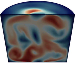
In figure 3 we show the spatial structure of the axisymmetric EVF at various values of the current. We show in figures 3(a) and 3(b) 3-D streamlines of the velocity field coloured by the magnitude of the velocity. The geometric organisation of the flow is similar to that of the von Kármán flows found in (Nore et al. Reference Nore, Tuckerman, Daube and Xin2003): the fluid is pumped along the axis from the equatorial plane towards the top and bottom caps; it is then expelled outwards along the two cylindrical caps and returns back to the equatorial plane along the side wall of the cell in a spiral fashion; the spiral motion of the fluid in the upper half of the cell is opposite to that of the fluid in the lower half. For $J = 5\ \textrm {A} \ \textrm {m}^{-2}$, the velocity field is stationary and $R_{\rm \pi}$ symmetric, meaning that

(3.1)\begin{equation} \left( \begin{array}{@{}c@{}} u_r \\ u_\theta \\ u_z \end{array} \right) (r,\theta,z) = \left( \begin{array}{@{}c@{}} u_r \\ -u_\theta \\ -u_z \end{array} \right) (r,-\theta,-z). \end{equation}

For $J = 500\ \textrm {A} \ \textrm {m}^{-2}$, the invariance under the $R_{\rm \pi}$ symmetry is broken and the streamlines of the velocity form a chaotic web. We show in figure 3(c) the magnitude of the velocity $\|\boldsymbol {u}\|$ in meridional planes for various values of the current $J$. For the smallest value of the current, $J = 0.1\ \textrm {A}\ \textrm {m}^{-2}$, the flow is steady and is the most intense near the rim of the electrical contact with the wires. Up until $J= 10 \ \textrm {A} \ \textrm {m}^{-2}$, the intensity of the flow gradually increases close to the vertical axis while still being invariant under the $R_{\rm \pi}$ symmetry. At $J = 50\ \textrm {A} \ \textrm {m}^{-2}$ and above this value the system becomes time dependent: the $R_{\rm \pi}$ symmetry is broken. The flow eventually becomes chaotic for large values of $J$. The intensity of the flow is notably small near the axis and in two regions close to the two contacts with the connecting wires.

Figure 3. Variable $J$, axisymmetric simulations. Spatial structure of the flow. (a,b) Streamlines coloured by the velocity magnitude in axisymmetric simulations for different values of $J$. (c) Transition of the axisymmetric flow as $J$ increases, visualized by the velocity magnitude $\|\boldsymbol {u}\|$ in the meridian plane.

The large change in the spatial structure of the flow between $J= 10 \ \textrm {A} \ \textrm {m}^{-2}$ and $J= 50 \ \textrm {A} \ \textrm {m}^{-2}$ indicates that a symmetry-breaking bifurcation occurs for a critical value $J_c$ in the interval $[10,50] \ \textrm {A} \ \textrm {m}^{-2}$. Figure 4(a) shows two snapshots of the magnitude of the velocity, $\| \boldsymbol {u} \|$, for $J = 50 \ \textrm {A}\ \textrm {m}^{-2}$. The flow is (quasi)-symmetric, (quasi)-steady and intense close to the axis at $t=4000\ \textrm {s}$, but steadiness is lost and the symmetry is broken at $t=30\ 000\ \textrm {s}$. Note also that at this time the magnitude of the velocity is small in a small cylinder close to the axis. To measure the critical current density $J_c^{axi}$ of the bifurcation, we calculate the volume average of the kinetic energy in the top half and in the bottom half of the cell. The volume average computed over the upper half is denoted $E_{top}$ and the volume average computed over the lower half is denoted $E_{bot}$. If, starting from $0$, the difference $|E_{top} - E_{bot}|$ grows in time, we conclude that there is a loss of symmetry. We use this quantity to measure the growth rate of the instability. This concept is illustrated in the inset of figure 4(b) where we show how $|E_{top} - E_{bot}|$ increases exponentially with time before reaching a plateau. Using a semi-logarithmic scale, we measure the growth rate $\lambda$ as the slope of the straight line fitting the growth of $|E_{top} - E_{bot}|$ in the transient regime. The growth rates computed with seven values of $J$ are shown in figure 4(b). Using linear extrapolation, we estimate that the instability threshold is $J_c^{axi}\approx 17\ \textrm {A\ m}^{-2}$.

Figure 4. Variable $J$, axisymmetric simulations. First bifurcation of the flow. (a) The $\| \boldsymbol {u} \|$ structure before and after the first bifurcation for $J= 50\ \textrm {A} \ \textrm {m}^{-2}$. (b) Growth rate $\lambda$ of the first axisymmetric instability as a function of $J$ and extrapolated threshold $J_c^{axi} =17\ \textrm {A\ m}^{-2}$. We measure the growth rate $\lambda$ from the time series for $|E_{top}-E_{bot}|$, the difference in kinetic energy between the top and bottom half of the fluid domain.

3.2. Variable $J$, 3-D study

We now present the results of 3-D simulations done with $M = 20$ or $M = 40$ Fourier modes. We focus on $M = 20$ and then justify why we use 20 modes by comparing cases with 20 and 40 modes.

In figure 5 we show the time evolution of the volume-averaged velocity $u$ and its Fourier components $u_0$, $u_1$, $u_2$, $u_3$. For $J=1\ \textrm {A} \ \textrm {m}^{-2}$, the system remains axisymmetric. At $J=5\ \textrm {A} \ \textrm {m}^{-2}$ a first symmetry-breaking bifurcation has occurred: the flow becomes three dimensional. The Fourier mode $m=2$ grows exponentially, saturates at $t= 20\ 000\ \textrm {s}$ and reaches a steady state at $t = 30000\ \textrm {s}$. For $J=10\ \textrm {A} \ \textrm {m}^{-2}$, a Hopf-like bifurcation has occurred: the mode $m=2$ remains dominant but the flow periodically oscillates. For $J=50\ \textrm {A} \ \textrm {m}^{-2}$, the transition to 3-D turbulence has occurred. Although the flow exhibits large 3-D fluctuations, the axisymmetric Fourier component $u_0$ remains dominant.

Figure 5. Variable $J$, 3-D simulations, $M = 20$. Time series of $u$ and modal content $u_0,u_1,u_2,u_3$ for different current densities $J$ as marked in the figures.

In figure 6(a) we show the time- and volume-averaged velocity $\bar {u}_{\textrm {3D}}$ of these 3-D simulations. For comparison, we also show in this graph the time- and volume-averaged velocity obtained in axisymmetric simulations; we use the symbol $\bar {u}_{{axi}}$ to differentiate it from the 3-D velocity. Inspection of the graph reveals that three dimensionalization appears between $J = 1$ and $5\ \textrm {A} \ \textrm {m}^{-2}$. For high current densities, we observe $\bar {u} \sim J^{1/2}$ or $J^{5/9}$. A fit of the curve on the three last points gives a slope of 0.51 for the axisymmetric simulations, which corresponds to the law $\bar {u}_{{axi}} \sim J^{1/2}$, and 0.55 for the 3-D ones, which corresponds rather to $\bar {u}_{\textrm {3D}} \sim J^{5/9}$. For medium current densities, the power law $\bar {u} \sim J^{2/3}$ is not incompatible with the data, but we cannot say that this scaling regime is clearly visible.

Figure 6. Variable $J,$ 3-D simulations, $M = 20$. (a) Variation of $\bar {u}$ with $J$ in axisymmetrical and 3-D simulations. (b) Ratio $\bar {u}_{\textrm {3D}} /\bar {u}_{{axi}}$ as a function of $J$.

We also note that the value of $\bar {u}_{\textrm {3D}}$ is just slightly below $\bar {u}_{{axi}}$, obtained assuming axisymmetry. This is also visible in figure 6(b) where we plot the ratio $\bar {u}_{\textrm {3D}}/\bar {u}_{{axi}}$ as a function of $J$. The flow is axisymmetric for very small values of the current (i.e. $\bar {u}_{3D} =\bar {u}_{{axi}}$). The ratio $\bar {u}_{\textrm {3D}}/\bar {u}_{{axi}}$ decreases as $J$ grows up to the value $J = 50\ \textrm {A} \ \textrm {m}^{-2}$, after which the ratio fluctuates around 0.8.

We show snapshots of the spatial organisation of the flow in figure 7 for the following three values of the current $J = 5,50,500\ \textrm {A} \ \textrm {m}^{-2}$. The flow is clearly three dimensional. This figure shows the value of $\| \boldsymbol {u} \|$ in a meridian plane and in the horizontal plane located at $z= 8.8 \ \textrm {cm}$. We observe that, for $J = 5\ \textrm {A} \ \textrm {m}^{-2}$, the equatorial symmetry by reflection is broken (there is a slight asymmetry between the lower and the upper half of the cell). Recall that the flow is time independent though. The flows for $J = 50\ \textrm {A} \ \textrm {m}^{-2}$ and $J = 500\ \textrm {A} \ \textrm {m}^{-2}$ are clearly turbulent. The large- and small-scale structures seem to be equally distributed throughout the domain. The low-speed region near the axis that is observed in the axisymmetric simulations for large values of $J$ (see figure 3c) is not present in these 3-D simulations.

Figure 7. Variable $J$, 3-D simulations, $M = 20$. Spatial structure of the flow: $\|\boldsymbol {u}\|$ for $J = 5,50,500 \ \textrm {A} \ \textrm {m}^{-2}$. The flow is steady for $J = 5\ \textrm {A} \ \textrm {m}^{-2}$ and turbulent for $J = 50, 500\ \textrm {A} \ \textrm {m}^{-2}$. Results are shown for (a) $J = 5\ \textrm {A} \ \textrm {m}^{-2}$, (b) $J = 50\ \textrm {A} \ \textrm {m}^{-2}$ and (c) $J = 500\ \textrm {A} \ \textrm {m}^{-2}$.

Because of the large fluctuations of the flow for high current densities, we can wonder if 20 modes are enough to properly represent the flow. For this reason, we have done a small convergence study varying the number of Fourier modes $M=20$ to $M=40$ and for increasing $J = 100,\ 500$ and $2000\ \textrm {A} \ \textrm {m}^{-2}$. On figure 8 we represent the time- and space-averaged modal kinetic energy $E_c$ as a function of $m$ for $M=20$ and $M=40$. For $J=100\ \textrm {A} \ \textrm {m}^{-2}$, the spectra show small differences above $m \geq 15$. For $J=500\ \textrm {A}\ \textrm {m}^{-2}$, we find similar differences from $m \geq 10$. In both simulations the most energetic modes are well converged and, hence, we can limit resolution to $M= 20$. For $J=2000\ \textrm {A} \ \textrm {m}^{-2}$, the spectra present more significant differences. The use of 40 modes is advisable in this case, since the azimuthal small scales are better resolved and certainly if the purpose is to access the fine turbulent structure of the flow. For the averaged velocity $\bar {u}$ however, 20 or 40 modes yield the same result. The plots of figure 6 obtained with $M=20$ remain valid up the highest value of $J$.

Figure 8. Variable $J$, 3-D simulations. Spectra of the kinetic energy averaged on time in the statistically steady state as a function of $m$ for $J = 100,\ 500,\ 2000 \ \textrm {A} \ \textrm {m}^{-2}$ and $M=20$ and $M=40$. The spectra show that 20 modes are sufficient for $J=100$ and $J=500\ \textrm {A} \ \textrm {m}^{-2}$, but for $J=2000\ \textrm {A} \ \textrm {m}^{-2}$, 40 modes are necessary to represent properly the first modes. Results are shown for (a) $J = 100\ \textrm {A} \ \textrm {m}^{-2}$, (b) $J = 500\ \textrm {A} \ \textrm {m}^{-2}$ and (c) $J = 2000\ \textrm {A} \ \textrm {m}^{-2}$.

In figure 9(a) we focus our attention on the steady state and 3-D flow obtained with $J = 5\ \textrm {A}\ \textrm {m}^{-2}$. Recall that this value of the current is above the critical threshold for which the axisymmetry is broken. We display in this figure several representations of the flow structure. Note that the flow organisation is strikingly similar to that observed in the von Kármán flows described in Nore et al. (Reference Nore, Tuckerman, Daube and Xin2003). We observe that the 3-D flow is also $R_{\rm \pi}$ symmetric (see (3.1)). The predominance of the Fourier mode $m=2$ is the spectral manifestation of the presence of two vortices roughly localized on the equatorial plane, rotating in the same direction, and with axes aligned with the directions $\{\theta = -{\rm \pi} /2, z=0\}$ and $\{\theta = {\rm \pi}/2,z=0\}$. The centre of one vortex is visible between the two red/orange oblong structures in the right panel in figure 9(c). The vortices are separated by a transition layer that is oblong, roughly localized on the equatorial plane and slightly twisted. This transition layer is materialised in the centre and the right panels in figure 9(c) by blue regions. The numerical simulations indicate that the 3-D steady state undergoes a second bifurcation in the interval $J \in [5,10] \ \textrm {A}\ \textrm {m}^{-2}$. Beyond the critical value, the flow starts oscillating periodically, but the overall structure of the flow stays $R_{\rm \pi}$ symmetric. The reader is invited to watch the video provided in the supplementary movie available at https://doi.org/10.1017/jfm.2022.779 to better appreciate the nature of this periodic flow. The simulation corresponding to the video is done with $J = 10 \ \textrm {A} \ \textrm {m}^{-2}$.

Figure 9. Variable $J$, 3-D simulations, $M = 20$. Flow after the first bifurcation for $J = 5\ \textrm {A} \ \textrm {m}^{-2}$. (a) Snapshots of $u_z$ at $z = -0.03$ m, $z = 0$ m and $z = 0.03$ m. (b) Contour of $\|\boldsymbol {u}\|$ taken for $\|\boldsymbol {u}\|$ =0.6 $\|\boldsymbol {u}\|_{max}$ coloured by $u_z$. (c) Snapshots of $\|\boldsymbol {u}\|$ at $r=0.8R$ for $-{\rm \pi} /2 \leq \theta \leq {\rm \pi}/2$ (left) and $0 \leq \theta \leq {\rm \pi}$ (right). One sees the $R_{\rm \pi}$ symmetry and the dominance of the $m=2$ azimuthal mode: there are two opposite vortices and two opposite aspiration fronts, where the flow is directed towards the centre of the cylinder.

A third bifurcation breaking the $R_{\rm \pi}$ symmetry occurs in the interval $J=[10,50] \ \textrm {A} \ \textrm {m}^{-2}$. Increasing the value of the current beyond this point quickly leads to a fully turbulent flow; see figure 7(c).

We determine the threshold of the first bifurcation (which we recall breaks the axisymmetry) by inspecting the time evolution of the modal volume-averaged values $u_m$ for $m=1,2,3$. Beyond the bifurcation threshold, some of these quantities start to grow exponentially. For instance, the inset of figure 10 shows that the Fourier components $u_1$ and $u_2$ grow exponentially in time. This technique allows us to measure the growth rates $\lambda$ of the modes $m=1,2$ for $J = 1,5,10\ \textrm {A} \ \textrm {m}^{-2}$. By linear fit we obtain $J_c^{ \rm 3D} \approx 2.5\ \textrm {A} \ \textrm {m}^{-2}$ for both modes $m=1$ and $m=2$. A similar observation was made for the first bifurcation of the von Kármán flow reported in Nore et al. (Reference Nore, Tartar, Daube and Tuckerman2004), where there is also a bifurcation of codimension two (the aspect ratio is $H/R\approx 1.64$ therein).

Figure 10. Variable $J$, 3-D simulations, $M = 20$. Threshold of the first bifurcation in three dimensions. Beyond a certain current density we observe exponential growth on $u_1$ and $u_2$, as shown in the inset at $J=5\ \textrm {A} \ \textrm {m}^{-2}$. The measured growth rates allow us to locate the threshold of the first 3-D bifurcation near $J_c^{ \rm 3D} \approx 2.5 \textrm {A} \ \textrm {m}^{-2}$ for both modes $m=1,2$.

3.3. Variable $B$, axisymmetric study

We now report the results obtained for a second series of numerical simulations where we investigate the influence of the magnitude of the imposed magnetic field. We use the same geometry of the cell as above, we fix $J=50 \ \textrm {A} \ \textrm {m}^{-2}$, and we use $\nu = 3.2\times 10^{-7} \ \textrm {m}^{2} \ \textrm {s}^{-1}$. Most simulations are done assuming axisymmetry. We have done one 3-D simulation at high field $B=10^{-1} \ \textrm {T}$ with $M=20$ modes. The other numerical parameters used for the simulations are reported in table 2.

Table 2. Numerical parameters for the axisymmetric simulations with variable $B$. Mesh size ${\rm \Delta} l$ (non-uniform meshes, smallest $\longrightarrow$ largest mesh size), time step ${\rm \Delta} t$, non-dimensional numbers $\overline {Re} = \bar {u} R / \nu$ and $\bar {\varPi } = \sigma \bar {u} B / J$.

We show in figure 11 the time- and volume-averaged velocity, $\bar {u}$, as a function of $B$. We observe that the behaviour of $\bar {u}$ is not monotone with respect to $B$: $\bar {u}$ first increases with $B$ and then sharply decays above a certain magnetic field strength. Power laws $\bar {u} \sim B^{2/3}$ followed by $\bar {u} \sim B^{1/2}$ and later $\bar {u} \sim B^{-1}$ are observed as $B$ increases.

Figure 11. Variable B, axisymmetric simulations. The typical flow magnitude $\bar {u}$ first increases with the magnetic field $B$, but decreases back again for very intense imposed magnetic fields.

Figure 12 shows snapshots of the magnitude of the electrical current density $\|\boldsymbol {j}\|$ and the magnitude of the velocity $\|\boldsymbol {u} \|$ for three values of the magnitude of the imposed magnetic field: $B=10^{-3}, 10^{-2}, 10^{-1}\ \textrm {T}$. In each panel of figure 12 the electrical current density is shown on the left and the magnitude of the velocity is shown on the right. We observe that the flow becomes steady as $B$ increases. For the largest value of $B$, we observe that the current density and the fluid motion are localised in a thin vertical cylinder whose two extremities coincide with the contact surfaces with the two wires supplying and extracting the current. In this case the flow is axisymmetric. We ran a 3-D simulation for $B=10^{-1}\ \textrm {T}$. The volume-averaged velocity $\bar {u}$ is the same in both axisymmetric and 3-D simulations (red point in figure 11), and the 3-D modes ($m \neq 0$) are zero. It seems that high $B$ makes the flow more axisymmetric. The reorganisation of the current density distribution in the cell and the drastic reduction of the fluid motion are due to the induction effects generated by the term $\sigma \boldsymbol {u} \times B \boldsymbol {e}_z$ in (2.1b).

Figure 12. Variable B, axisymmetric simulations, $J=50 \ \textrm {A} \ \textrm {m}^{-2}$. The spatial structure of the current density (left) and of the magnitude of the velocity (right) varies significantly when the intensity of the magnetic field increases. For the lowest value of $B$, the flow is turbulent and the current density is barely influenced by inductive effects ($\sigma \boldsymbol {u} \times B \boldsymbol {e}_z$). For the largest value of $B$, the induction effects are strong. The flow becomes steady and due to the induction effects the electrical current almost goes in straight lines from the top wire to the bottom wire. The current density is scaled from yellow to purple in the range [0,$J_w$], where $J_w=1250\ \textrm {A} \ \textrm {m}^{-2}$ is the imposed current density in the wires.

Note also that we do not observe any Shercliff or Hartmann boundary layers at high magnetic field as in duct flows (Hunt & Stewartson Reference Hunt and Stewartson1965; Moresco & Alboussiere Reference Moresco and Alboussiere2004) in this set-up. Such layers are always localised near the solid boundaries of the domain and channel the electrical current when the Hartmann number

(3.2)\begin{equation} Ha = B R \left ( \frac{\sigma}{\rho \nu} \right )^{1/2} \end{equation}

is large. Here $Ha \approx 4,40,400$ for the three simulations reported in figure 12, and does increase from left to right. But in our case the current density and imposed magnetic field are roughly parallel whereas they are perpendicular in the case of duct flows.

3.4. Variable $\nu$, axisymmetric study

We now explore the influence of the viscosity. We fix $J = 50\ \textrm {A}\ \textrm {m}^{-2}$, $B = 1\ \textrm {mT}$, and we artificially vary the viscosity $\nu$ of the liquid metal. Usually, the viscosity of a liquid metal is between $10^{-7}$ and $10^{-6}\ \textrm {m}^{2}\ \textrm {s}^{-1}$, but we extend the study to other non-realistic viscosities in order to better understand the flow's behaviour. Only axisymmetric simulations are done. The other numerical parameters used for the simulations are reported in table 3. We focus our attention on the influence of the viscosity on the time- and volume-averaged velocity, $\bar {u}$. The results of these simulations in the range $\nu \in [8{\times } 10^{-8}, 3{\times } 10^{-5}]\ \textrm {m}^{2}\ \textrm {s}^{-1}$ are shown in figure 13. For small values of the viscosity, it seems that $\bar {u} \sim \nu ^{-1/9}$ or $\nu ^{0}$ as in (1.2). When the viscosity is large, we observe $\bar {u} \sim \nu ^{-1}$, which is a clear indication of the Stokes regime.

Table 3. Numerical parameters for the axisymmetric simulations with variable $\nu$. Mesh size ${\rm \Delta} l$ (non-uniform meshes, smallest $\longrightarrow$ largest mesh size), time step ${\rm \Delta} t$, non-dimensional numbers $\overline {Re} = \bar {u} R / \nu$ and $\bar {\varPi } = \sigma \bar {u} B / J$.

Figure 13. Variable $\nu$, axisymmetric simulations. Velocity $\bar {u}$ as a function of the viscosity $\nu$. The slope asymptotes between 0 and $-1/9$ for low viscosities and to $-1$ for high viscosities.

3.5. One master curve for the intensity of flow in the inductionless regime

We have deliberately chosen in the previous sections to report all the results in dimensional form to make clear that the effects of increasing $J$ and increasing $B$ are not always equivalent. This difference is mainly due to inductive effects. If $U$ is a typical velocity, we can estimate that induction is not important as long as

(3.3)\begin{equation} \varPi = \frac{\sigma U B}{J} \ll 1. \end{equation}

In this inductionless regime, we can group all our previous measures of flow intensity using a non-dimensional representation. A natural scale for velocity in the inertial regime is $(JB R/\rho )^{1/2}$ and with it, we can define a Reynolds number as

(3.4)\begin{equation} Re_{in} = \left(\dfrac{J B}{\rho}\right)^{1/2} \dfrac{R^{3/2}}{\nu}, \end{equation}

which only depends on input parameters (hence, subscript $in$). In figure 14 we plot $\overline {Re} = \bar {u} R / \nu$, the Reynolds number based on the measured velocity as a function of $Re_{in}$ for the axisymmetric simulations that meet the requirement (3.3) (we only take the data in the range $B\in [0,2]\ \textrm {mT}$ for the simulations with varying $B$). It is remarkable that all the data points collapse on a single curve. At high $Re_{in}$, we observe not unexpectedly that $\overline {Re} \sim Re_{in}$.

Figure 14. Computed Reynolds number $\overline {Re} = \bar {u} R / \nu$ as a function of input parameter Reynolds numbers $Re_{in}$ defined in (3.4).

3.6. Scaling laws for swirling EVFs

All our simulations were done in the limit $\varGamma = {\mu _0 J R}/{B} \ll 1$, where the EVF always has a strong swirling character. Here we explain the different scaling regimes of such swirling EVFs. We introduce $[\boldsymbol {u} ] = U$, $[\boldsymbol {j} ] = J$ and $[\boldsymbol {b}] = B$ as typical scales of velocity, current density and magnetic field.

We start with the large $B$, inductive regime. When induction, i.e. the term $(\sigma \boldsymbol {u}{\times } \boldsymbol {b})$, is important in Ohm's law, the Lorentz force acts as a magnetic brake on the bulk flow (Hunt & Malcolm Reference Hunt and Malcolm1968). We conjecture that saturation of flow magnitude occurs when this bulk magnetic braking balances the inductionless part of the Lorentz force with magnitude $JB$. This balance implies that

(3.5)\begin{equation} U \sim \frac{J }{ \sigma B} \quad \mbox{(inductive)} \end{equation}

or $\varPi \sim 1$. This scaling law is coherent with what we observed at high $B$.

When induction is not important, when $\varPi \ll 1$, we can imagine three possible regimes: viscous, intermediate and inertial. For very weak Lorentz forces, the Lorentz force can be balanced by the viscous forces, $[\rho \nu \nabla ^{2} \boldsymbol {u} ] \sim [\boldsymbol {j} \times \boldsymbol {b}]$. In this Stokes regime the flow occupies the entire cell, so we can use $[\boldsymbol {r}] = R$ as the length scale. From this balance we then find that

(3.6)\begin{equation} U \sim \dfrac{J B R^{2}}{\rho \nu}, \quad \text{(inductionless, viscous).}\end{equation}

This viscous regime was clearly visible in our simulations when the flow speed was at its lowest.

For the highest flow intensities, inertia will be dominant in opposing the Lorentz force. Naively speaking, we can simply balance $[\rho ( \boldsymbol {u}\ \boldsymbol{\cdot }\ {\boldsymbol {\nabla }} ) \boldsymbol {u}] \sim [ \boldsymbol {j} \times \boldsymbol {b}]$ and, using somewhat arbitrarily $[\boldsymbol {r}] = R$ as the length scale, we then find that

(3.7)\begin{equation} U \sim \left( \dfrac{J B R}{\rho} \right)^{1/2}, \quad \text{(inductionless, inertial 1/2).} \end{equation}

A more elaborate analysis of the torque balance between the boundary and the bulk (Davidson Reference Davidson1992; Davidson et al. Reference Davidson, Kinnear, Lingwood, Short and He1999) yields

(3.8)\begin{equation} U \sim \left(\dfrac{J B R}{\rho} \right)^{5/9} \left( \frac{R}{\nu} \right )^{1/9} , \quad \text{(inductionless, inertial 5/9).} \end{equation}

The inertial regime was clearly visible in our simulations, but we cannot conclude which exponent, $1/2$ or $5/9$, is more adapted.

An intermediate regime can sometimes be observed when the viscous effects, the inertial effects and the Lorentz force are all of the same intensity. This is possible because forcing mainly occurs near the electrical contact, in the viscous boundary layer. The scaling law for this intermediate regime is derived in Herreman et al. (Reference Herreman, Nore, Cappanera and Guermond2021). Using the $z$ component of the vorticity equation, the three-term balance requires that $[ (\boldsymbol {u}\ \boldsymbol{\cdot }\ \boldsymbol {\nabla }) \omega _z - (\boldsymbol {\omega }\ \boldsymbol{\cdot }\ \boldsymbol {\nabla }) u_z ] \sim [ \rho ^{-1} B \partial _z j_z ] \sim [ \nu \partial _{zz}^{2} \omega _z ]$. In a boundary layer of width $\delta$ near the electrical contacts with the wires, we estimate $[\partial _z] = \delta ^{-1}$ and $[\partial _r ]= R^{-1}$. If $[u_r, u_\theta ] = U$ then $[u_z] = U \delta R^{-1}$ due to incompressibility. This yields the estimates $[ \omega _r, \omega _\theta ] = U \delta ^{-1}$ and $[\omega _z] = U R^{-1}$ for the vorticity. Inserting these scales in the three-term balance, we obtain two equivalence relations ${U^{2}}/{R^{2}} \sim {JB}/{\rho \delta } \sim {\nu U}/{R \delta ^{2}}$, from which, after eliminating $\delta$, we find that

(3.9)\begin{equation} U \sim \left(\dfrac{J B}{\rho} \right)^{2/3} \dfrac{R}{\nu^{1/3}}, \quad \text{(inductionless, laminar boundary layer)}, \end{equation}

where the power law $U \sim J^{2/3}$ was clearly visible in the simulations of Herreman et al. (Reference Herreman, Nore, Cappanera and Guermond2021), it is much less visible in the present set-up. We think that this may be due to the fact that the von Kármán-like flow, driven here, is rather unstable and easily turbulent in the bulk. If turbulent flow structures reach into the boundary layer, the latter will no longer remain laminar and this will break the subtle three-term balance. In Appendix A) we show that the $2/3$ scaling can also be derived from the model of Davidson (Reference Davidson1992), if one uses a laminar friction law for the viscous stress, which is equivalent to supposing a laminar boundary layer.

4.1. Variable wire radius $R_w$

As in § 3, we fix the geometry of the cell to be $(R,H,H_w)=(10,18,4)\ \textrm {cm}$ and vary both the radius $R_w$ of the connecting wires and the current density $J$. We expect the intensity of the fluid flow generated by the electrovortex to be a decreasing function of the ratio $R_w/R$ (Bojarevičs et al. Reference Bojarevičs, Freibergs, Shilova and Shcherbinin1989).

We show in figure 15(a) the space-averaged velocity $u$ as a function of time for the following four values of the ratio $R_w/R$: $0.2, 0.4, 0.6, 0.8$, and with $J = 500\ \textrm {A} \ \textrm {m}^{-2}$. These simulations are done assuming axisymmetry. As expected, both the time average of $u$ and the time fluctuations of $u$ increase as the ratio $R_w/R$ decreases. In figure 15(b) we show $\bar {u}$ as a function of $R_w/R$ for the following five values of $J$: $5, 50, 100, 500, 2000\ \textrm {A} \ \textrm {m}^{-2}$. In figure 15(c) we show $u_{bar}$ as a function of J for the following four values of $R_w/R$: 0.2, 0.4, 0.6, 0.8. Here again, we observe that the flow intensity decreases monotonically as $R_w/R$ increases. This observation holds for all the values of the current.

Figure 15. Variable $R_w$, axisymmetric simulations. Global measures. (a) Time series of the velocity $u$ for different $R_w/R$ and $J = 500\ \textrm {A} \ \textrm {m}^{-2}$. Plot of $\bar {u}$ as (b) a function of $R_w/R$ for different $J$, and (c) a function of $J$ for different $R_w/R$. The mean velocity increases with $J$ and decreases with $R_w/R$ and all curves present similar trends.

In figure 16 we show snapshots of $\|\boldsymbol {u}\|$ for the following four values of the ratio $R_w/R$: $0.2, 0.4, 0.6, 0.8$ with $J = 500\ \textrm {A} \ \textrm {m}^{-2}$. One axisymmetric and one fully 3-D simulation have been done for each value of $R_w/R$. Three-dimensional simulations have been computed with $M=20$, as justified in § 3.2. In the axisymmetric simulations (top panels), we always observe a cylindrical region where the fluid is approximately at rest. The diameter of this cylindrical region coincides with that of the connecting wires. In the corresponding 3-D simulations (bottom panels), this low-speed cylindrical core is absent and the flow is overall more turbulent. The flow speed remains close to that of the axisymmetric simulations.

Figure 16. Variable $R_w$, axisymmetric and 3-D simulations. Snapshots of the velocity field $\|\boldsymbol {u}\|$ for $J = 500\ \textrm {A} \ \textrm {m}^{-2}$ and different $R_w/R$. Top row: axisymmetric simulations; bottom row: 3-D simulations. In axisymmetrical simulations we observe low speeds in a cylinder with radius $R_w$. In 3-D simulations such a low-speed region is less visible and turbulent structures are present everywhere.

It is tempting to try to model the dependence of the typical flow speed on $R_w/R$. For non-swirling EVFs ($B=0$), ad hoc fitting laws are given by Vlasyuk (Reference Vlasyuk1987) and Chudnovskii (Reference Chudnovskii1989) proposed a theoretical model based on a meridional contour integral. Unfortunately, one cannot generalize the method of Chudnovskii (Reference Chudnovskii1989) to swirling EVFs. In Appendix B we approximately calculate the torque that the Lorentz force exerts on the bottom half of the fluid domain and how it depends on $R_w$. This calculation requires $b_\theta$ right above the electrical contact and we use the $b_\theta$ profile that is observed with Millere boundary conditions (Millere et al. Reference Millere, Sharamkin and Shcherbinin1980; Herreman et al. Reference Herreman, Nore, Ziebell Ramos, Cappanera, Guermond and Weber2019) or above a uniform current inlet. This yields torques

(4.1)\begin{equation} K = K_0 \begin{cases} 1 - (4R^{2}_w/3R^{2}) & \text{(Millere)}, \\ 1 - R^{2}_w/R^{2} & \text{(uniform)}, \end{cases} \end{equation}

with $K_0 = \frac 14 I B R^{2}$. Both expressions give a parabolic decay of the torque as $R_w/ R$ increases. We compare in figure 17(a) these two expressions with the actual torque obtained from the numerical simulations. We observe that the model based on Millere's approximation is very accurate in the range $R_w/R\in [0,0.5]$. We now estimate the dependence of the intensity of the flow motion, $U$, with respect to $R_w/R$, by assuming $U$ is proportional to torques

(4.2)\begin{equation} U \approx U_0 \begin{cases} 1 - (4R^{2}_w/3R^{2}) & \text{(Millere)}, \\ 1 - R^{2}_w/R^{2} & \text{(uniform)}. \end{cases} \end{equation}

Here $U_0$ is the maximum of $U$ in the limit $R_w/R \rightarrow 0$. We show in figure 17(b) the quantity $\bar {u}/ {u}_0$ as a function of $R_w/R$. We also show in this figure the two theoretical profiles $1 - \alpha (R^{2}_w/R^{2})$ with $\alpha =4/3$ and $1$. We have estimated ${u}_0$ by fitting the parabola $\bar {u} = {u}_0 ( 1 - \beta (R_w/R)^{2} )$ to the data shown in figure 15(b). This shows that the estimation of the velocity dependence on $R_w/R$ can be quite accurate for intermediate $J$. However, we do observe that the parabolic profile does not fit very well the data when $J$ is very small, a linear profile fits better the data in this limit (see figure 17c).

Figure 17. Model for the geometrical dependence of flow intensity on wire radius. (a) Normalized torque $K/K_0$ as a function of $R_w/R$. The Millere model works really well for $R/R_w < 0.6$. (b) Normalized velocity $\bar {u}/{u}_0$ as a function of $R_w/R$ for high $J$. The orange zone corresponds to the zone between the two theoretical profiles, uniform and Millere. The fit of the velocity works well. (c) Normalized velocity $\bar {u}/{u}_0$ for low $J$. A linear fit seems more accurate for these low current densities.

4.2. Variable height $H$

Up until now, all simulations were done in a cell with aspect ratio $H/R=1.8$. We now vary $H/R$ and study how this affects the flow. We run axisymmetric simulations where we vary $H$ for several values of the current density $J$ and keep $(R,R_w,H_w)=(10,2,4) \ \textrm {cm}$.

In figure 18(a) we show the time history of the volume-averaged velocity observed in simulations done with the aspect ratios $H/R=0.5, 1.0, 1.8$ and with the current density $J = 500 \textrm {A} \ \textrm {m}^{-2}$. We observe that the larger $H/R$, the larger $u$ and the larger the fluctuations of $u$. In figure 18(b–c) we show the quantities $\bar {u}$ and $\bar {u}_{max}$ as functions of $J$ for the three considered aspect ratios. The time- and space-averaged velocity scales like $\bar {u} \sim J^{1/2}$ for large values of $J$ for the three values of $H/R$ investigated. The maximal speed $\bar {u}_{max}$ behaves in a slightly different manner. We observe that $\bar {u}_{max}$ is independent of $H/R$ when $J$ is large. The power law $\bar {u}_{max} \sim J^{1/2}$ seems to apply when $H/R$ is large, whereas the power law $\bar {u}_{max} \sim J^{2/3}$ seems a better fit when $H/R$ is small. With lower $H/R$, we observe that the flow is less turbulent (weaker oscillations are, for example, visible in figure 18(a) at $H/R=0.5$). This probably explains why the $2/3$, laminar boundary layer scaling law applies better in cylinders with a low aspect ratio $H/R$.

Figure 18. Variable $H$, axisymmetric simulations. (a) Time series of $u$ for different aspect ratios and $J = 500\ \textrm {A} \ \textrm {m}^{-2}$. The higher the cell is, the more intense and fluctuating the flow is. Plots of (b) $\bar {u}$ and (c) $\bar {u}_{max}$ as a function of $J$. The scaling law 1/2 is observed for each aspect ratio for $\bar {u}$, but it changes when one looks at $\bar {u}_{max}$, where the scaling law 2/3 is better adapted to cells with a smaller aspect ratio.

Figure 19 shows the spatial distribution of $\|\boldsymbol {u}\|$ in the meridian section for the two current densities $J = 5, 500\ \textrm {A} \ \textrm {m}^{-2}$ and for the three aspect ratios $H/R=0.5, 1.0, 1.8$. The flow is time independent for the smallest value of the current density $J = 5\ \textrm {A} \ \textrm {m}^{-2}$, but it is turbulent for the larger value $J = 500\ \textrm {A} \ \textrm {m}^{-2}$. When the aspect ratio is small, i.e. $H/R=0.5$, the fluid motion is somewhat restricted to a small region close to the vertical axis.

Figure 19. Variable $H$, axisymmetric simulations. Snapshots of $\|\boldsymbol {u}\|$ for (a) $J = 5\ \textrm {A} \ \textrm {m}^{-2}$ and (b) $J = 500 \textrm {A} \ \textrm {m}^{-2}$. In cells with small aspect ratios, the flow does not reach the high $r$ regions. The flow remains localized above and below the electrical contact.

This localisation will bias the spatial average in $\bar {u}$ and this likely explains the difference in behaviour of $\bar {u}$ and $\bar {u}_{max}$ observed in figure 18(b–c).

4.3. Symmetrical vs asymmetrical wires

In our set-up, current is injected and withdrawn using a symmetrical pair of wires with the same diameter $R_w$. This is different from the asymmetrical cell simulated in Herreman et al. (Reference Herreman, Nore, Cappanera and Guermond2021), that only has one thin wire extracting current at the bottom. We investigate the effect of this symmetrical or asymmetrical current injection by comparing two cells with different connections. We set $R=10 \ \textrm {cm}$ for both cells. In the first cell we fix the aspect ratio to be $H/R =1$ and we use connecting wires at the top and bottom of the cell with the same radius and height $(R_w,H_w)=(2,4) \ \textrm {cm}$. For the second cell, we set $H/R=0.5$ and we use only one thin wire at the bottom of the cell with $(R_w,H_w)=(2,4) \ \textrm {cm}$. The current density is supposed uniform and equal to $J$ at the top lid as in Herreman et al. (Reference Herreman, Nore, Cappanera and Guermond2021). All the simulations are axisymmetric. We fix $B = 1\ \textrm {mT}$ and $\nu = 3.2\times 10^{-7} \ \textrm {m}^{2} \ \textrm {s}^{-1}$, and we vary $J$.

In figure 20(a) we show the typical velocity magnitude $\bar {u}$ observed in the two configurations as a function of $J$. It appears that $\bar {u}$ is significantly higher in the asymmetrical set-up than in the symmetrical one. For large values of the current, we observe that $\bar {u} \sim J^{1/2}$ in the symmetrical set-up, but in the asymmetrical set-up we observe the laminar boundary layer scaling law, $\bar {u} \sim J^{2/3}$, just as in Herreman et al. (Reference Herreman, Nore, Cappanera and Guermond2021). This suggest that the flows are radically different in both configurations, so let us compare their spatial structure.

Figure 20. Symmetrical and asymmetrical set-ups. (a) Time- and space-averaged magnitude of the velocity $\bar {u}$ as a function of $J$ in both set-ups. (b) Snapshots of $\|\boldsymbol {u}\|$ in the symmetrical cell $H/R=1$ and the asymmetrical cell $H/R=0.5$.

In figure 20(b) we compare snapshots of $\|\boldsymbol {u}\|$ in the asymmetrical and symmetrical set-ups for three values of $J$. At low $J$, the flows are quite comparable in both configurations. The only real difference is the velocity on the axis which is almost zero in the asymmetrical cell contrary to the symmetrical one. For higher $J$, there are significant differences in the flow structure. In the case $J= 50 \ \textrm {A} \ \textrm {m}^{-2}$, the flow is localized near the axis in the symmetrical set-up, but fills the entire cell in the asymmetrical one. For $J= 500 \ \textrm {A} \ \textrm {m}^{-2}$, the flow in the symmetrical cell has a vertical structure that is significantly more turbulent. We think that this increased turbulence is due to the mixing layer that is present in the equatorial plane of the symmetrical set-up but is absent in the asymmetrical set-up. Such an equatorial mixing layer loses its stability fairly easily in von Kármán flows (Nore et al. Reference Nore, Tuckerman, Daube and Xin2003, Reference Nore, Tartar, Daube and Tuckerman2004) and here this seems to be just the same. The $2/3$ scaling regime likely requires a not too turbulent flow in the bulk.