2.1. Average along homogeneity directions

Here, we explore the specific configuration of a temporally evolving shear layer with two homogeneity directions in the streamwise $x$ and spanwise directions $z$ (see § 3). Therefore, planar averages over the set of points $\mathbb {P}(Y) = \{ X, Y, Z | Y, 0 \leq X \leq L_x, 0 \leq Z \leq L_z \}$ can be used in place of ensemble averages; $L_x$ and $L_z$ represent the size of the averaging domain in the streamwise and spanwise directions, respectively. Equations (2.2a) and (2.2b) then reduce to

(2.3a)\begin{align} \underbrace{\partial_t \left\langle \left( \delta {\phi} \right)^2 \right\rangle_{\mathbb{P}}}_{\textrm{d}t\ \textrm{term}} &= \underbrace{- \boldsymbol{\nabla}_{\boldsymbol{r}} \cdot \left\langle {(\delta {\boldsymbol{u}}) \left(\delta \phi\right)^2} \right\rangle_{\mathbb{P}}}_{r\text{-}\textrm{Transfer}} \underbrace{- {\partial}_{Y} \left\langle {(\sigma v') \left(\delta \phi\right)^2} \right\rangle_{\mathbb{P}} }_{Y\text{-}\textrm{Transfer}}, \end{align}

(2.3b)\begin{align}\underbrace{\partial_t \left\langle \left( \delta {\phi'} \right)^2 \right\rangle_{\mathbb{P}}}_{\textrm{d}t\ \textrm{term}} &= \underbrace{- \boldsymbol{\nabla}_{\boldsymbol{r}} \cdot \left\langle {(\delta {\boldsymbol{u}}) \left(\delta \phi'\right)^2} \right\rangle_{\mathbb{P}}}_{r\text{-}\textrm{Transfer}} \underbrace{- 2 \left\langle {(\delta \phi')(\delta v')} \right\rangle_{\mathbb{P}} {\partial}_{r_y} \left\langle \delta \phi \right\rangle_{\mathbb{P}} }_{r\text{-}\textrm{Production}}\notag\\ &\quad \underbrace{- \partial_Y \left\langle \left(\sigma v'\right) \left(\delta \phi'\right)^2 \right\rangle_{\mathbb{P}}}_{Y\text{-}\textrm{Transfer}} \underbrace{- 2 \left\langle {(\delta \phi')(\sigma v')} \right\rangle_{\mathbb{P}} {\partial}_{Y} \left\langle \delta \phi \right\rangle_{\mathbb{P}} }_{Y\text{-}\textrm{Production}}, \end{align}

where we have used $\langle v \rangle _{\mathbb {P}} = 0$ and hence $v = v'$. Equation (2.3a) is the transport equation for the second-order structure function of the total field $\phi$. It reveals that time variations of $\langle (\delta \phi )^2\rangle _\mathbb {P}$ are due to the combined effect of two transfer processes (more precisely divergence of fluxes) which occur concomitantly in scale $\boldsymbol {r}$ and physical space ${Y}$. The transfer in scale space, abbreviated by the $r$-transfer term, quantifies the direction and amplitude of the cascade process, i.e. the transfer of the quantity $\langle (\delta \phi )^2 \rangle _{\mathbb {P}}$ between different orientations and the modulus of the vector $\boldsymbol {r}$. Hereafter, in this paper, the word ‘cascade’ will be used to designate the transfer of ‘energy’ between scales which is mathematically given by the $r$-divergence term in (2.3a) and (2.3b). The other transfer term, abbreviated $Y$-transfer, represents the transport of a given liquid scale in geometrical space, i.e. from one position within the flow (here, one $Y$ plane location) to another.

Equation (2.3b) pertains to the fluctuating component $\phi '$. In addition to similar transfer terms, the latter contains two additional processes, namely two production processes which again act concomitantly in scale and physical space. The production process is associated with the presence of inhomogeneities, i.e. some gradients of liquid volume fraction $\langle \phi \rangle _{\mathbb {P}}$. As was proved by Thiesset et al. (Reference Thiesset, Duret, Ménard, Dumouchel, Reveillon and Demoulin2020), this production mechanism can also be interpreted as an exchange of liquid between the mean and the fluctuating fields which acts to homogenize the mean volume fraction field. Further physical interpretations and algebraic decompositions of the different terms of (2.3a) and (2.3b) are provided by Thiesset et al. (Reference Thiesset, Duret, Ménard, Dumouchel, Reveillon and Demoulin2020) but are not considered in the present study.

Note here again that (2.3a) and (2.3b) hold even if the flow is anisotropic and inhomogeneous.

2.2. Average over all directions of the separation vector

The different terms of (2.3a) and (2.3b) have argument list ($\boldsymbol {r}, Y, t)$, i.e. a five-dimensional (5-D) problem. The dependence of the statistics on the separation vector $\boldsymbol {r}$ embeds the anisotropic character of the transport of liquid, which is of major importance in this flow. However, substantial information can first be gained by averaging over all orientations of the separation vector $\boldsymbol {r}$, thereby reducing the problem complexity to a 3-D problem with argument list ($|\boldsymbol {r}|, Y, t)$. This can be achieved in two fashions. The first method is to perform an angular average over all solid angles. This operation is denoted $\langle \bullet \rangle _\varOmega$ and is defined by

(2.4)\begin{equation} \langle \bullet \rangle_\varOmega = \frac{1}{4{\rm \pi}} \iint_\varOmega \bullet \sin \theta \,\textrm{d}\theta \,\textrm{d} \varphi, \end{equation}

where the set of solid angles $\varOmega = \{ \varphi , \theta ~|~ 0 \leq \varphi \leq {\rm \pi}, 0 \leq \theta \leq 2 {\rm \pi}\}$ with $\varphi = \arctan (r_y/r_x)$ and $\theta = \arccos (r_z/|\boldsymbol {r}|)$. The angular average is related to the spherical average within a sphere of radius $r = |\boldsymbol {r}|$, noted $\langle \bullet \rangle _\mathbb {S}$ and defined by (Hill Reference Hill2002; Thiesset et al. Reference Thiesset, Duret, Ménard, Dumouchel, Reveillon and Demoulin2020)

(2.5)\begin{equation} \langle \bullet \rangle_\mathbb{S} = \frac{3}{4{\rm \pi} r^3} \iiint_\mathbb{S} \bullet r^2 \sin \theta\,\textrm{d} \theta\,\textrm{d} \varphi\,\textrm{d} r = \frac{3}{r^3} \int_0^r \langle \bullet \rangle_\varOmega r^2 \,\textrm{d}r. \end{equation}

2.3. Average along the inhomogeneity direction

Finally, a spatial average can further be performed. In our case, the latter operates on the $Y$ direction and writes

(2.6)\begin{equation} \langle \bullet \rangle_\mathbb{Y} = \frac{2}{L_y} \int_\mathbb{Y} \bullet \,\textrm{d} Y \end{equation}

with $\mathbb {Y} = \{ Y | -L_y/4 \leq Y \leq L_y/4 \}$ ($Y=0$ is located at the shear layer centreline). Using the gradient theorem, averaging over $\mathbb {Y}$ allows us simplifying the Y-Transfer terms as follows

(2.7a)\begin{gather} \left\langle \partial_Y \left\langle \left(\sigma v'\right) \left(\delta \phi\right)^2 \right\rangle_{\mathbb{P}} \right\rangle_{\mathbb{Y}} = \left\langle \left(\sigma v'\right) \left(\delta \phi\right)^2 \right\rangle_{\mathbb{P}(Y = {L_y}/{4})} - \left\langle \left(\sigma v'\right) \left(\delta \phi\right)^2 \right\rangle_{\mathbb{P}(Y ={-}({L_y}/{4}))}, \end{gather}

(2.7b)\begin{gather}\left\langle \partial_Y \left\langle \left(\sigma v'\right) \left(\delta \phi^\prime\right)^2 \right\rangle_{\mathbb{P}} \right\rangle_{\mathbb{Y}} = \left\langle \left(\sigma v'\right) \left(\delta \phi^\prime\right)^2 \right\rangle_{\mathbb{P}(Y = {L_y}/{4})} - \left\langle \left(\sigma v'\right) \left(\delta \phi^\prime\right)^2 \right\rangle_{\mathbb{P}(Y ={-}({L_y}/{4}))}. \end{gather}

2.4. Summary

In summary, roughly speaking, an angular (spatial) average enables studying the time/scale/space transport of liquid structures independently of their orientations (position in the flow). Consequently, these different averaging procedures have the advantage of reducing the problem complexity but this is automatically accompanied by a loss of information which can be summarized as follows.

1. (i) $\langle \bullet \rangle _{\mathbb {P}}$ leads to a problem in five dimensions, with argument list $(\boldsymbol {r}, Y, t)$. It corresponds to the more general version of the equations in the temporally evolving shear layer with $x$ and $z$ being the homogeneity directions.

2. (ii) $\langle \bullet \rangle _{\mathbb {P}, \varOmega }$ yields a problem in three dimensions, with argument list $(r, Y, t)$, the information about the preferential orientation (anisotropy) of the liquid structures is lost.

3. (iii) $\langle \bullet \rangle _{\mathbb {P}, \varOmega , \mathbb {Y}}$ corresponds to a 2-D problem, with argument list $(r, t)$, the information about the locality within the flow is lost.

In the present paper, for the sake of pedagogy, we start by considering the most simplified version of the problem (angularly and spatially averaged budgets) and then successively lift some averaging operations up to the more general version of the two-point transport equations. Most of the present analysis is rendered feasible thanks to data from numerical simulations. In the following sections, we describe the simulation code and database.

3.1. The ARCHER code

The liquid–gas shear flow is simulated using the high-performance-computing code ARCHER developed at the CORIA laboratory (Ménard, Tanguy & Berlemont Reference Ménard, Tanguy and Berlemont2007). It is based on the one-fluid formulation of the incompressible Navier–Stokes equation which is solved on a Cartesian mesh, viz.

(3.1)\begin{equation} \partial_t \rho \boldsymbol{u} + \boldsymbol{\nabla} \cdot \left( \rho \boldsymbol{u} \otimes \boldsymbol{u} \right) ={-} \boldsymbol{\nabla} p + \boldsymbol{\nabla} {\cdot} (2 \mu \boldsymbol{\mathsf{D}}) + \boldsymbol{f} + \gamma \mathcal{H} \delta_s \boldsymbol{n}. \end{equation}

Here, $p$ is the pressure field, $\boldsymbol{\mathsf{D}}$ the strain rate tensor, $\boldsymbol {f}$ a source term, $\mu$ the kinematic viscosity, $\rho$ the density, $\gamma$ the surface tension, $\boldsymbol {n}$ the unit normal vector to the liquid–gas interface, $\mathcal {H}$ its mean curvature and $\delta _s$ is the Dirac function characterizing the location of the liquid–gas interface. For solving (3.1), the convective term is written in conservative form and solved using the improved Rudman (Reference Rudman1998) technique presented in Vaudor et al. (Reference Vaudor, Ménard, Aniszewski, Doring and Berlemont2017). The Sussman et al. (Reference Sussman, Smith, Hussaini, Ohta and Zhi-Wei2007) method is used to compute the viscous term. To ensure incompressibility of the velocity field, a Poisson equation is solved. The latter accounts for the surface tension force and is solved using a multigrid preconditioned conjugate gradient algorithm (Zhang Reference Zhang1996) coupled with a ghost-fluid method (Fedkiw et al. Reference Fedkiw, Aslam, Merriman and Osher1999).

A coupled level-set and volume-of-fluid solver is used for transporting the interface, the level-set function accurately describing the geometric features of the interface (its normal and curvature) and the volume-of-fluid function ensuring mass conservation. The density is calculated from the volume of fluid (or liquid volume fraction) as $\rho = \rho _l \phi + \rho _g(1-\phi )$, where $\rho _l, \rho _g$ is the density of the liquid and gas phase. The dynamic viscosity ($\mu _l$ or $\mu _g$) depends on the sign of the level-set function. In cells containing both a liquid and a gas phase, a specific treatment is performed to evaluate the dynamic viscosity, following the procedure of Sussman et al. (Reference Sussman, Smith, Hussaini, Ohta and Zhi-Wei2007). For more information about the ARCHER solver, the reader can refer to e.g. Ménard et al. (Reference Ménard, Tanguy and Berlemont2007), Duret et al. (Reference Duret, Luret, Reveillon, Ménard, Berlemont and Demoulin2012) and Vaudor et al. (Reference Vaudor, Ménard, Aniszewski, Doring and Berlemont2017).

3.2. Numerical domain and flow features

The flow configuration is that of a planar liquid layer being sheared by a gas stream. The flow is directed towards the $x$ axis, and $z$ denotes the spanwise and $y$ the vertical axis, respectively. The calculation domain is $L_x \times L_y \times L_z = 8 \times 4 \times 4\ \textrm {{cm}}^{3}$ in the streamwise, vertical and spanwise directions, respectively. The liquid and gas properties correspond to those of water and air at ambient pressure. The dynamic viscosity $\mu$ ($\textrm {kg}\ \textrm {m}^{-1}\ \textrm {s}^{-1}$) is $\mu _l = 1.0 \times 10^{-3}$ and $\mu _g = 1.8 \times 10^{-5}$ for the liquid and gas phases, respectively. The fluid density $\rho$ ($\textrm {kg}\ \textrm {m}^{-3}$) is $\rho _l = 1.0 \times 10^{3}$ and $\rho _g = 1.2$, respectively. The surface tension $\gamma = 0.072\ \textrm {N}\ \textrm {m}^{-1}$.

Close to the liquid–gas interface, an error function profile for the streamwise velocity $u$ is initially prescribed and is given by

(3.2)\begin{equation} u(x,y,z) = \frac{u_g}{2} \left[1+ \text{erf} \left\{ 86.83 \left(\frac{y}{L_y} -\frac{1}{2} \right) \right\} \right]. \end{equation}

The spanwise $w$ and vertical v velocity components $v(x,y,z) = w(x,y,z) = 0$. $u_g = 7.5 \ \textrm {m}\ \textrm {s}^{-1}$ denotes the maximum gas velocity. The constant $86.83$ corresponds to a vorticity thickness of $\delta _\omega = 1.15\ \textrm {{mm}}$. This was set so that the most unstable wavelength of the Kelvin–Helmholtz instability is expected to be half of $L_x$ and the spanwise Rayleigh–Taylor instability has a wavelength of approximately $L_z/6$ (Marmottant & Villermaux Reference Marmottant and Villermaux2004). These two modes were forced in the present simulation by superimposing on the liquid–gas interface a small sinusoidal perturbation with period $L_x/2$ and $L_z/6$ in the streamwise and spanwise directions, respectively. This was done to trigger the destabilization of the liquid layer and consequently reduce the overall computational time. The initialized level-set function $G$ was set as follows:

(3.3)\begin{equation} G(x,y,z) = \left(\frac{L_y}{2}-y\right) + \frac{L_y}{200} \left[ \sin \left(4 {\rm \pi}\frac{x}{L_x}\right) + \sin \left(12 {\rm \pi}\frac{z}{L_z}\right) \right]. \end{equation}

Periodic boundary conditions are used in the streamwise and spanwise direction. A no-slip boundary condition is applied to the bottom frontier while an outflow condition is used at the uppermost boundary of the calculation domain. The mesh size consisted of $N_x \times N_y \times N_z = 512 \times 256 \times 256$ cells and 1024 processors were used. This corresponds to a cell size $\Delta x = \Delta y = \Delta z \approx 0.156\ \textrm {mm}$. The question of the adequacy of a given resolution depends on the physical quantity of interest. Indeed, the resolution needed for some large-scale quantities, such as the turbulent kinetic energy or the liquid volume fraction, to be grid independent is most likely not the same as the one needed for some small-scale quantities (e.g. the enstrophy) to be faithfully resolved. As emphasized in subsequent sections, the budgets given by (2.3a) and (2.3b) will be proved to be nicely closed proving that the present resolution is adequate, at least as far as the liquid–gas interface properties are concerned.

The initial Weber number based on the gas velocity $u_g$ and the shear-layer vorticity thickness $\delta _\omega$ is $We_g = \rho _g u_g^2 \delta _\omega / \gamma = 1.08$. As per Taguelmimt, Danaila & Hadjadj (Reference Taguelmimt, Danaila and Hadjadj2016), we define the Reynolds number by use of the average dynamic viscosity, i.e. $Re =2 u_g \delta _\omega / (\nu _g + \nu _l) = 1078$.

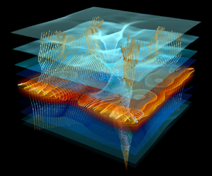
Typical snapshots of the flow simulation are presented in figure 2. The overall phenomenology of this flow is quite similar to what is commonly referred to as an air-assisted atomization process, as documented by e.g. Lasheras & Hopfinger (Reference Lasheras and Hopfinger2000), Marmottant & Villermaux (Reference Marmottant and Villermaux2004) and Fuster et al. (Reference Fuster, Matas, Marty, Popinet, Hoepffner, Cartellier and Zaleski2013). The rapid destabilization of the liquid–gas interface is observed to be followed by the oblique ejection of ligaments, which subsequently break into a myriad of droplets. Qualitatively, one observes that the degree of tortuousness of the liquid–gas interface is increasing from $t^* = 0.98$ up to $t^* = 1.37$ and then becomes smoother at $t^* = 1.83$. Further, while liquid structures manifest mainly as ligaments at $t^* = 0.98$ and $t^* = 1.37$, some detached droplets are clearly identified at $t^* = 1.83$. The break-up mechanism thus occurs between $t^* = 1.37$ and $t^* = 1.83$. Still, at $t^* = 1.83$, the interface separating the liquid and gas phases located near the centreline of the shear layer is experiencing a relaxation mechanism most likely attributable to the increasing influence of surface tension relative to the decreasing shear rate. This flow configuration thus reveals some multi-scale features and a concomitant transport of the liquid phase in scale and flow position space. It is therefore a very nice candidate for being explored with two-point statistical equations. However, it is worth stressing that the present simulation reveals a much less complex physics than the one presented by e.g. Fuster et al. (Reference Fuster, Matas, Marty, Popinet, Hoepffner, Cartellier and Zaleski2013) and Ling et al. (Reference Ling, Fuster, Zaleski and Tryggvason2017, Reference Ling, Fuster, Tryggvason and Zaleski2019). Indeed, the liquid–gas interface being forced with perturbations of finite amplitude probably bypasses some mechanisms revealed in a striking manner by Ling et al. (Reference Ling, Fuster, Zaleski and Tryggvason2017, Reference Ling, Fuster, Tryggvason and Zaleski2019) using very detailed simulations. Here, the focus of the paper is mostly on discussing the potential of two-point statistics to extract some information about a given flow and we do not pretend that the simulation configuration presented here can be considered as representative of real liquid-sheet shear-induced atomization configurations.

Figure 2. Typical snapshots of the simulation. The flow is from left to right. The liquid–gas interface is initially perturbed with a sinusoidal pattern which promotes the destabilization of the flow, thereby reducing the overall computational cost. From (a–c) $t^*= tL_x/u_g = 0.98, 1.37, 1.83$.

For assessing the two-point budgets which will be described in the subsequent section, we saved the velocity, the level-set and the volume of fluid fields for 90 time steps during the simulation, each separated by $3.75\times 10^{-4}\ \textrm {s}$. This ensured that the time derivative terms were accurately estimated. Two-point statistics were computed using an in-house Python/Fortran code which makes use of a hybrid OpenMP–MPI parallelization. Structure functions were calculated in the range of scales $- L_y/2 \leq (r_x, r_y, r_z) \leq L_y/2$ so that the large-scale dynamics of the flow is well captured. This imposes the minimum and maximum reachable positions for the mid-point $Y$, as the coordinates $y^+ = \max (Y) + \max (r_y)/2$ and $y^- = \min (Y) + \min (r_y)/2$ should stay within the computational domain, i.e. stay within the interval $(-L_y/2 ; L_y/2)$. Choosing $- L_y/2 \leq (r_x, r_y, r_z) \leq L_y/2$, leads to $-L_y/4 \leq Y \leq L_y/4$ as represented in figure 3.

Figure 3. Representation of the maximum and minimum reachable positions for the mid-point $Y$.

Contrary to Thiesset et al. (Reference Thiesset, Dumouchel and Ménard2019a, Reference Thiesset, Duret, Ménard, Dumouchel, Reveillon and Demoulin2020), the angular averages were here preferred to the spherical average. The reason is that $\langle \bullet \rangle _\varOmega$ relies only on a double integral which, given the size of the present database, yields substantial reduction of the computational effort. This operation is performed as follows. First, each two-point quantity at a given plane $Y$ is interpolated from Cartesian $(r_x, r_y, r_z)$ to spherical coordinates $(r, \theta , \phi )$ using the radial basis function ‘Rbf’ algorithm of the SciPy-interpolation library. We employed a linear radial basis function. Then, the double integral was calculated using the ‘dblquad’ method of the SciPy-integration library. The overall database represents approximately 0.9 TB and approximately 250 000 CPU hours were necessary for the simulation and post-processing. Given this quite high number of computational resources, we considered here only one set of parameters. The library employed here to compute two-point statistics could be substantially optimized using the methodology described by Gatti et al. (Reference Gatti, Remigi, Chiarini, Cimarelli and Quadrio2019). Hence, we expect to be able, in the short term, to reduce significantly this amount of computational time to post-process larger simulation domains.

Instead of investigating an inhomogeneous and time-evolving shear layer, one could have thought of a simpler homogeneous configuration for which a steady state could have been possibly reached. The first that comes to mind is homogeneous sheared turbulence, as was recently addressed by Rosti et al. (Reference Rosti, Ge, Jain, Dodd and Brandt2019). This flow can potentially reach a steady state, hence the time derivative terms in (2.2a) and (2.2b) are zero. This flow is further homogeneous, i.e. the gradient of mean liquid volume fraction is zero and hence the two production terms in (2.2b) are zero. The transfer in $\boldsymbol {X}$-space can also be proven to be zero using the Green–Ostrogradski theorem (see (B5) of Thiesset et al. Reference Thiesset, Duret, Ménard, Dumouchel, Reveillon and Demoulin2020). By difference, the only remaining term (the $r$-transfer) is also zero. Hence, homogeneous sheared two-phase flows leads to the very simple conclusion that all terms in the budget are zero. This conclusion is quite obvious given that a stationary flow configuration means that liquid structures have reached statistical equilibrium and hence there is no transfer between scales or between different positions within the flow. Consequently, this configuration, which is very common when dealing with shear turbulence, does not allow us to extract any relevant information about the statistical behaviour of liquid–gas shear turbulence. Note also that the steady state can only be achieved artificially in the case of a bounded numerical domain (e.g. Pumir Reference Pumir1996). Otherwise, the turbulent length scales and kinetic energy grow in time. Another configuration is Taylor–Couette flow, for which the presence of the wall on the upper and lower boundaries yields the exact same conclusions. In addition, it requires handling the interaction (the contact) between the liquid and the sliding walls, which could lead to numerical complexities. Because the present study focuses on the phase indicator (a scalar field), one can further think of a configuration similar to homogeneous scalar mixing in forced turbulence fed by a uniform scalar gradient (e.g. Yeung, Donzis & Sreenivasan Reference Yeung, Donzis and Sreenivasan2005, and references therein). Here again, a steady state is achieved only using a bounded domain. This additionally requires imposing a uniform liquid gradient in the domain, which appears hardly feasible numerically. In addition, since $\phi$ is a non-diffusive scalar, (there is no diffusion term in the transport equation for $\phi$), the dissipation of $\phi$ variance is zero. It is thus not even sure that, in this situation, the statistics of $\phi$ reach a steady state in bounded domains as there is no dissipative process (except maybe a surface tension effect) to compensate for $\phi$ scalar production. To conclude, all these configurations, though attractive, may reveal more drawbacks than advantages.

4.1. Relation to the correlation function

Straightforward calculations allow us to write the second-order structure function in terms of the correlation function, viz.

(4.1)\begin{equation} \left\langle(\delta \phi)^2 \right\rangle_{\mathbb{E}} = \left\langle\phi^2(\boldsymbol{x}^+ ) \right\rangle_{\mathbb{E}} + \left\langle\phi^2(\boldsymbol{x}^- ) \right\rangle_{\mathbb{E}} - 2 \left\langle\phi(\boldsymbol{x}^+ )\phi(\boldsymbol{x}^- ) \right\rangle_{\mathbb{E}}. \end{equation}

The right-most term on the right-hand side of (4.1) is the correlation function of the phase indicator. It is worth stressing that this is not the first time that the correlation function of the indicator function has been defined. Indeed, it is widely used for characterizing porous media (Debye, Anderson Jr & Brumberger Reference Debye, Anderson and Brumberger1957; Adler, Jacquin & Quiblier Reference Adler, Jacquin and Quiblier1990; Torquato Reference Torquato2002, to cite but a few), colloids (Grimson Reference Grimson1983) and fractal aggregates (Sorensen Reference Sorensen2001). For all these physical situations, it is used as an indicator of the geometrical features of the pore or aggregate structure. The correlation function of the phase indicator can also be experimentally measured through the use of small-angle-scattering techniques, which opens up nice perspectives in the context of two-phase flows. This remains far beyond the scope of the present study.

Equation (4.1) reveals that, for a homogeneous medium, i.e. for which $\langle \phi ^2(\boldsymbol {x}^+ ) \rangle _{\mathbb {E}} = \langle \phi ^2(\boldsymbol {x}^- ) \rangle _{\mathbb {E}} = \langle \phi \rangle _{\mathbb {E}}$, the large-scale limit of the phase indicator structure function is (see Thiesset et al. Reference Thiesset, Duret, Ménard, Dumouchel, Reveillon and Demoulin2020)

(4.2)\begin{equation} \lim_{r \to \infty} \langle (\delta \phi)^2 \rangle_{\mathbb{E}} = 2 \langle \phi \rangle_{\mathbb{E}} - 2\langle \phi \rangle_{\mathbb{E}}^2 = 2 \langle \phi \rangle_{\mathbb{E}} (1-\langle \phi \rangle_{\mathbb{E}}). \end{equation}

This can be readily demonstrated by recalling that the correlation function $\langle \phi (\boldsymbol {x^+}) \phi (\boldsymbol {x^-}) \rangle _{\mathbb {E}}$ asymptotes to the value $\langle \phi \rangle _{\mathbb {E}}^2$ at large scales (Fitzhugh Reference Fitzhugh1983). In very diluted media, i.e. $\langle \phi \rangle _{\mathbb {E}} \ll 1$, the limit value at large scales is thus $2\langle \phi \rangle _{\mathbb {E}}$. In the inhomogeneous case, it depends on the volume fraction at points $\boldsymbol {x^+}$ and $\boldsymbol {x^-}$ and on the way the autocorrelation $\langle \phi (\boldsymbol {x^+}) \phi (\boldsymbol {x^-}) \rangle _{\mathbb {E}}$ varies with respect to $\boldsymbol {r}$. It is not even sure that, in this situation, $\langle (\delta \phi )^2 \rangle _{\mathbb {E}}$ tends towards a plateau at large scales. Hence, the physical interpretation of the large-scale limit of $\langle (\delta \phi )^2 \rangle$ in inhomogeneous cases is much more complex. In what follows, we present a simple case where the limit at large scales can be obtained even though the medium is inhomogeneous.

4.2. Geometrical representation of the phase indicator two-point statistics

Further, $(\delta \phi )^2 (\boldsymbol {X}, \boldsymbol {r})$ can be interpreted by resorting to some geometrical reasoning. From the definition of $(\delta \phi )^2 (\boldsymbol {X}, \boldsymbol {r})$ and figure 1, one easily remarks that, when the points $\boldsymbol {x}^+$ and $\boldsymbol {x}^-$ lie together within the liquid or gas phase, then $(\delta \phi )^2$ is zero. On the contrary, $(\delta \phi )^2$ is activated as soon the phases found at the two points $\boldsymbol {x}^+$ and $\boldsymbol {x}^-$ are different. Consequently, $(\delta \phi )^2$ measures the scale/space distribution of jumps between the two phases.

Further insights into the physical meaning of the structure and correlation functions can be gained by recalling that the spatial average over $\boldsymbol {x}$ of the correlation function $\phi (\boldsymbol {x}) \phi (\boldsymbol {x} + \boldsymbol {r})$ is the convolution of $\phi (\boldsymbol {x})$ with its translated version at a distance $\boldsymbol {r}$, $\phi (\boldsymbol {x}+ \boldsymbol {r})$ (Sorensen Reference Sorensen2001). Geometrically, it thus reads as the intersection of the ensemble $E^- = \{ \boldsymbol {x} \in \mathbb {R} | \phi (\boldsymbol {x}) = 1 \}$ with the ensemble $E^+=\{ \boldsymbol {x} \in \mathbb {R} | \phi (\boldsymbol {x} + \boldsymbol {r})=1 \}$, which can conveniently be written $E^- \cap E^+$. Analogously, the spatially averaged structure function of $\phi$ can be defined as the symmetric difference (disjunctive union) of the ensemble $E^-$ with the ensemble $E^+$, or $E^- \triangle E^+$.

This is illustrated in figure 4 in the case of a single closed set. It is seen that, when $|\boldsymbol {r}| \to 0$, the structure function (orange zones) tends to zero while the correlation function (green zones) is equal to the volume of $E^-$, which is here $\langle \phi \rangle _{\mathbb {R}}$. When the separation $|\boldsymbol {r}|$ is larger than the extent of $E^-$, the opposite is observed: the correlation function is zero while the structure function is equal to the volume of $E^-$ plus the volume of $E^+$, i.e. twice the volume of $E^-$, or $2 \langle \phi \rangle _{\mathbb {R}}$. As said previously for homogeneous cases, the structure function tends towards $2\langle \phi \rangle _{\mathbb {R}}(1-\langle \phi \rangle _{\mathbb {R}})$ at large scale. For the case presented in figure 4, there is only one structure surrounded by an arbitrarily large volume, and hence $\langle \phi \rangle _{\mathbb {R}} \ll 1$ so that the structure function tends towards a plateau whose value is obtained by the limit $2\langle \phi \rangle _{\mathbb {R}}(1-\langle \phi \rangle _{\mathbb {R}}) \to 2 \langle \phi \rangle _{\mathbb {R}}$.

Figure 4. Graphical representation of the spatially averaged phase indicator correlation function (green) and structure function (orange) given $\phi (\boldsymbol {x})$ (blue) and $\phi (\boldsymbol {x}+\boldsymbol {r})$ (yellow).

For intermediate scales, the intersection and symmetric difference of $E^-$ with $E^+$ depends on the morphology of the media under consideration. For instance, it is extremely well known from the literature dedicated to porous media that the two-point statistics of the phase indicator are often used to assess information about the tortuousness of the interface (Adler et al. Reference Adler, Jacquin and Quiblier1990; Torquato Reference Torquato2002, and references therein). Similarly, the fractal facets of aggregates are often appraised by use of correlation function of the phase indicator at intermediate scales (see e.g. Sorensen Reference Sorensen2001). In particular, Morán et al. (Reference Morán, Fuentes, Liu and Yon2019) showed that, when increasing the ratio between the largest scales (the aggregate radius of gyration) and the smallest scales (the radius of the primary particle), the correlation function reveals an increasing range of scales complying with a fractal scaling (a power law). When several structures are present, it also depends on the way the different liquid structures are organized in space.

When $|\boldsymbol {r}|$ is small, figure 4 reveals that $E^- \triangle E^+$ delineates the contours of $E^-$. It is thus expected that $(\delta \phi )^2 (\boldsymbol {X}, \boldsymbol {r})$ is related to the surface area for small values of the separation $r$. A more specific discussion on this aspect is detailed in the next subsections.

To summarize, the phase indicator correlation function provides information about the liquid volume, morphology/tortuousness and surface area at large, intermediate and small scales, respectively. In this regard, two-point statistics of the phase indicator field thus appear as a nice candidate for asserting the multi-scale features of the liquid/gas interface. In the next subsections, we provide more details on this aspect.

4.3. Small-scale expansion of the structure function

In Thiesset et al. (Reference Thiesset, Duret, Ménard, Dumouchel, Reveillon and Demoulin2020), the authors came up with the fortunate observation that, in the limit of small $|\boldsymbol {r}|$,

(4.3)\begin{equation} \lim_{r \to 0} \langle (\delta \phi)^2 \rangle_{\mathbb{R},\mathbb{S}} \propto \langle \varSigma \rangle_{\mathbb{R}} r, \end{equation}

where $\langle \varSigma \rangle _{\mathbb {R}}$ is the surface density defined as the amount of surface of the liquid–gas interface within the computational domain $\mathbb {R} \in \{ X,Y,Z \}$. Therefore, it appears that $(\delta \phi )^2$ contains information about the geometry of the liquid–gas interface, namely its surface area. Here again, this observation should be interpreted in the light of previous works dedicated to heterogeneous media.

In this respect, the wide literature pertaining to porous media (Torquato Reference Torquato2002, for instance) discusses in great detail the relationship between the small-scale limit of the correlation function and the surface density. This question dates back to the work by Debye et al. (Reference Debye, Anderson and Brumberger1957), who addressed the special case of isotropic and homogeneous fields, for which correlation functions depend only on $r = |\boldsymbol {r}|$. Once written in terms of the second-order structure function, they proved that

(4.4)\begin{equation} \lim_{r \to 0} \langle (\delta \phi) ^2\rangle_\mathbb{E} = \frac{\langle \varSigma \rangle_{\mathbb{E}} r}{2}. \end{equation}

Equation (4.4) can be readily derived using the same methodology as the one used to solve the Buffon needle problem. Hence, the derivation is quite straightforward. Later, Kirste & Porod (Reference Kirste and Porod1962) and Frisch & Stillinger (Reference Frisch and Stillinger1963) extended the analysis to the next order and proved that, for isotropic–homogeneous media, and by further assuming that the interface separating the two phases is of class $C^2$

(4.5)\begin{equation} \langle (\delta \phi) ^2\rangle_\mathbb{E} = \frac{\langle \varSigma \rangle_{\mathbb{E}} r}{2} \left[ 1- \frac{r^2}{8} \left( \langle \mathcal{H}^2\rangle_{0, \mathbb{E}} - \frac{\langle \mathcal{G}\rangle_{0, \mathbb{E}}}{3} \right) \right] + {O}(r^5). \end{equation}

Here, $\mathcal {H}$ and $\mathcal {G}$ are the mean and Gaussian curvatures, respectively, and $\langle \bullet \rangle _{0, \mathbb {E}}$ denotes an area weighted average. Note that there is no square terms in (4.5). Ciccariello (Reference Ciccariello1995) showed that for smooth surfaces, all even-order terms in the expansion of $\langle (\delta \phi ) ^2\rangle$ with respect to $r$ vanish. Wu & Schmidt (Reference Wu and Schmidt1971) and Ciccariello (Reference Ciccariello1995) provided the next $r^5$ and $r^7$ terms in the expansion, which are not added here for the sake of simplicity.

When the medium is anisotropic yet homogeneous, Berryman (Reference Berryman1987) proved that (4.4) remains valid when the (anisotropic) correlation function is angularly averaged. To better understand this result, it is worth noting that, since the geometrical variables appearing in (4.5) are intrinsic to the interface, they are invariant to rotation and translation. The angular average can thus be thought of as being equivalent to an average operation over several randomly oriented structures characterized by the same surface density and curvature. Similarly, the spatial average is equivalent to calculating an average over several randomly located, yet geometrically equivalent, structures. Therefore, it is worth testing if the third-order expansion (4.5), which was derived rigorously for isotropic homogeneous media, applies to anisotropic inhomogeneous media after application of an angular and a spatial average.

4.4. Assessment of geometrical measures using synthetic fields

For doing this, we consider the simple toy model of a spheroid characterized by its eccentricity $e = \sqrt {1-(a/c)^2}$ ($a$ is the semi-axis and $c$ is the distance from centre to pole), placed in the centre of a domain. We consider different values for the eccentricity $e= 0\,\%, 58\,\%, 70\,\%, 87\,\%$ by modifying the value of $c$ while keeping $a$ constant. This obviously results in different degrees of anisotropy. In addition, the spheroid being placed at the centre of a wider domain, the field is also inhomogeneous. Two-point statistics are obtained by averaging over space $\mathbb {R} = \{ X,Y,Z \}$ and further angularly averaged as per (2.4). Results are presented in figure 5. It is observed that, at small scales, spatially and angularly averaged structure functions perfectly match the ‘homogenized’ and ‘isotropized’ version of (4.5) which writes

(4.6)\begin{equation} \langle (\delta \phi) ^2\rangle_{\mathbb{R}, \varOmega} = \frac{\langle \varSigma \rangle_{\mathbb{R}} r}{2} \left[ 1- \frac{r^2}{8} \left( \langle \mathcal{H}^2\rangle_{0,\mathbb{R}} - \frac{\langle \mathcal{G}\rangle_{0,\mathbb{R}}}{3} \right) \right] + {O}(r^5). \end{equation}

The area weighted Gaussian curvature was here estimated by use of the Gauss–Bonnet theorem, i.e. ${S_{sph}}\langle \mathcal {G}\rangle _{0,\mathbb {R}} = 4 {\rm \pi}$, where $S_{sph}$ is the surface area of a spheroid. The value of $\langle \mathcal {H}^2\rangle _{0,\mathbb {R}}$ was estimated numerically by using the routines described by Essadki et al. (Reference Essadki, Drui, Larat, Ménard and Massot2019) and Di Battista et al. (Reference Di Battista, Bermejo-Moreno, Ménard, de Chaisemartin and Massot2019) now available through the project Mercur(v)e (http://docs.mercurve.rdb.is/). Further, when increasing the eccentricity, both the slope at small scales (recall that $a$ is kept constant) and the limiting value at large $r$ increase. Figure 5 further shows that (4.6) holds very nicely up to a separation $r \approx 2 a$. Kirste & Porod (Reference Kirste and Porod1962) and Frisch & Stillinger (Reference Frisch and Stillinger1963) proved that (4.5) should hold up to a separation $r$ equal to twice the ‘reach’ of the surface, the ‘reach’ being defined as the minimal normal distance from the surface to the medial axis (Federer Reference Federer1959). In the present case, the latter is close to $a$. It is also verified that the second-order structure function can be used to estimate the geometrical properties of the liquid field, namely its volume (limit at large $r$ which is $2\langle \phi \rangle _{\mathbb {R}}$), its surface density (first-order expansion at small scales) and a measure of surface curvature $\langle \mathcal {H}^2\rangle _{0,\mathbb {R}} - {\langle \mathcal {G}\rangle _{0,\mathbb {R}}}/{3}$ (third-order expansion at small scales). Results are gathered in table 1, where estimates obtained by the structure function perfectly match those obtained either analytically (volume, surface area and area weighted Gaussian curvature) or numerically (for $\langle \mathcal {H}^2 \rangle _{0,\mathbb {R}}$) using the routines of Essadki et al. (Reference Essadki, Drui, Larat, Ménard and Massot2019) and Di Battista et al. (Reference Di Battista, Bermejo-Moreno, Ménard, de Chaisemartin and Massot2019). The maximum error is for $\langle \mathcal {H}^2\rangle _{0,\mathbb {R}} - {\langle \mathcal {G}\rangle _{0,\mathbb {R}}}/{3}$, for which the departure from the theoretical prediction is very limited (approximately 1 %). The surface area and volume are within less than a per cent.

Figure 5. Angularly averaged structure functions of the phase indicator field for prolate spheroids with different eccentricities (anisotropies) $e = \sqrt {1-(a/c)^2} = 0\,\%, 58\,\%, 70\,\%, 87\,\%$ ($a$ is the semi-axis and $c$ is the distance from centre to pole). Symbols corresponds to the direct estimation and lines are given by (4.6).

Table 1. Comparison of theoretical values for the volume, surface density and curvature (bold font) to those inferred from the limiting behaviour of $\langle (\delta \phi )^2\rangle _\mathbb {R}$ at either large or small scales (normal font). The error is given within the parantheses.

Equation (4.6) is further tested for a planar geometry ($\mathcal {G}=0$) with two facing interfaces perturbed with a controlled multi-scale sinusoidal perturbation. We have considered four cases, with (a) one, (b) three, (c) four and (d) five forcing wavelengths, respectively. For case (a), the period is equal to $L_x$, for (b) the periods are $L_x$, $2L_x$ and $4L_x$. For (c), we had a fourth sinusoid with period $8L_x$. For (d), a fifth wavelength is added with period equal to $16L_x$. Their respective amplitudes are kept constant ($\equiv L_y/64$) and their phases are shifted by $2 {\rm \pi}/ 10$. The resulting phase indicator fields are portrayed in figure 6. It is readily shown that increasing the number of sinusoids increases the tortuousness and the scale content of the interface. It also results in a decrease of the reach of the media, i.e. the minimal normal distance from surface to the medial axis decreases. Hence, it is expected that the range of scales over which (4.6) applies shortens from (a) to (d).

Figure 6. (a–d) The phase indicator field of four sinusoidally perturbed media and (e) their respective angularly averaged structure functions. The dashed lines correspond the numerical estimation of the scale distribution and the full lines represent the theoretical expression given by (4.6).

The angularly averaged second-order structure functions for these four fields are portrayed in figure 6. We have made the choice of normalizing the separation $r$ by the surface density to appraise the scaling $\langle (\delta \phi )^2\rangle _{\mathbb {R}, \varOmega }$ at small scales. Scrutinizing this particular range of scales, one observes that the collapse is very well satisfied, proving again that the first-order expansion of (4.6) applies well. Pushing the analysis to the third order, figure 6 reveals that (4.6) applies satisfactorily for case (a) and (b) and over a narrower portion of scales when moving from case (c) to (d). This simply translates to the diminution of the reach.

Travelling along larger scales where (4.6) no longer applies, the different curves depart from each other when increasing the tortuousness of the interface. This indicates that, as expected, the structure function contains information about the morphology of the media under consideration which differs significantly from case (a) to case (d). We also point out that increasing the scale content of the interface (the number of sinusoids), results in broader distributions of $\langle (\delta \phi ) ^2\rangle _{\mathbb {R}, \varOmega }$. This shows that the second-order structure function has great potential for appraising the multi-scale features of heterogeneous media and thus appears to be a nicely tailored tool for characterizing two-phase flows in particular.

In summary, using synthetic fields, we have emphasized a close relationship between the second-order structure functions at small scales and the geometrical properties of the interface (surface area and curvatures). At very large scales, it provides a measure of liquid volume. At intermediate scales (larger than the reach but smaller than the extent of the typical liquid structures), the structure function provides information about the morphology of the medium and its scale content. Therefore, the reach of the surface plays an important role here as it separates the range of scales for which geometry applies (viz. $\varSigma$, $\mathcal {H}$ and $\mathcal {G}$ together with (4.6) are sufficient to describe the media under consideration) and the range of scales for which two-point statistics become a morphological descriptor (Torquato Reference Torquato2002) for which both the geometry and the additional information about the medial axis are required for the structure to be characterized. For scales larger than the reach, the separation $r$ should be referred to as the morphological parameter, as is generally done in morphological analysis using e.g. integral geometrical measures (Minkowski functional) of parallel sets (Arns, Knackstedt & Mecke Reference Arns, Knackstedt and Mecke2004).

By virtue of (2.5), (4.6) implies

(4.7)\begin{equation} \langle (\delta \phi) ^2\rangle_{\mathbb{R}, \mathbb{S}} = \frac{3 \langle \varSigma \rangle_\mathbb{R} r}{8} \left[ 1- \frac{r^2}{12} \left( \langle \mathcal{H}^2\rangle_{0, \mathbb{R}} - \frac{\langle \mathcal{G}\rangle_{0, \mathbb{R}}}{3} \right) \right] + {O}(r^5). \end{equation}

In Thiesset et al. (Reference Thiesset, Duret, Ménard, Dumouchel, Reveillon and Demoulin2020), it was observed that a prefactor of $1/3$ should be preferably used in (4.7) instead of the value of $3/8$. The origin of this difference was not yet explained. By re-analysing the data of Thiesset et al. (Reference Thiesset, Duret, Ménard, Dumouchel, Reveillon and Demoulin2020), it appeared that this difference is attributed to the post-processing procedure and particularly an imprecise estimation of spherical averages at small scales. Indeed, in Thiesset et al. (Reference Thiesset, Duret, Ménard, Dumouchel, Reveillon and Demoulin2020), use was made of a simple (and computationally light) linear interpolation for transforming two-point statistics from Cartesian to spherical coordinates which was the source of the error. Here, the radial basis function algorithm is used instead with a much more accurate estimation, thereby confirming that the prefactor in (4.7) is indeed $3/8$.

Another difference between the present work and that of Thiesset et al. (Reference Thiesset, Duret, Ménard, Dumouchel, Reveillon and Demoulin2020) is the scalar field which is employed as being representative of the liquid phase. Thiesset et al. (Reference Thiesset, Duret, Ménard, Dumouchel, Reveillon and Demoulin2020) considered the two-point equation for the liquid volume fraction whereas, here, the phase indicator is used instead. The latter field can take only 0 or 1 values while the former can take any value between 0 and 1 in cells containing an interface. When the mesh cell size goes to zero, the liquid volume fraction tends to the phase indicator. The motivation for the choice of phase indicator is that comparisons are here made with some theoretical elaborations (Berryman Reference Berryman1987; Kirste & Porod Reference Kirste and Porod1962; Frisch & Stillinger Reference Frisch and Stillinger1963) pertaining to porous media, whose description is made on the basis of the phase indicator but not the (solid) volume fraction. Another argument in favour of the colour-function field is the dependence of the two-point statistics of the liquid volume fraction field on the numerical resolution. For more details on this aspect, the reader is referred to the technical report of Thiesset & Poux (Reference Thiesset and Poux2020).

4.5. Assessment of geometrical measures in the shear layer

Equation (4.6) can further be generalized by lifting the spatial average. In this case, $\langle (\delta \phi )^2 \rangle _\varOmega$ is expected to relate to the local values of $\varSigma , \mathcal {H}^2 , \mathcal {G}$. For the shear-layer flow considered in the present study, this can be written as

(4.8)\begin{equation} \langle (\delta \phi) ^2\rangle_{\mathbb{P}, \varOmega} = \frac{\langle \varSigma \rangle_{\mathbb{P}} r}{2} \left[ 1- \frac{r^2}{8} \left( \langle \mathcal{H}^2\rangle_{0, \mathbb{P}} - \frac{\langle \mathcal{G}\rangle_{0, \mathbb{P}}}{3} \right) \right] + {O}(r^5), \end{equation}

where $\langle \varSigma \rangle _{\mathbb {P}}$, $\langle \mathcal {H}^2\rangle _{0, \mathbb {P}}, \langle \mathcal {G}\rangle _{0, \mathbb {P}}$, which depend on $Y$ and $t$, are respectively the surface density, the area weighted average of $\mathcal {H}^2$ and $\mathcal {G}$ within a volume of size $L_x L_z \Delta y$.

In figure 7 we compare the values of $\langle \varSigma \rangle _{\mathbb {P}}$ as estimated directly from the zero level-set surface (we used the routines described by Di Battista et al. Reference Di Battista, Bermejo-Moreno, Ménard, de Chaisemartin and Massot2019; Essadki et al. Reference Essadki, Drui, Larat, Ménard and Massot2019) or from the limit to small scales of $2 \langle (\delta \phi ) ^2\rangle _{\mathbb {P}, \varOmega }/r$. The agreement is nearly perfect, with the absolute difference within less than a per cent, confirming that (4.8) holds with a very nice degree of confidence. The agreement is also verified for the spatially averaged values of $\langle \varSigma \rangle _{\mathbb {P}, \mathbb {Y}}$. Again, the difference between the two methods is within a per cent (see figure 7). Here, the analysis was carried out only for the first-order expansion of (4.8) and did not incorporate the dependence on the $r^3$ term. The reason is that the flow is populated by some rather small liquid structures with a small local radius of curvature. Hence, since (4.8) is expected to hold up to a separation $r/2$ smaller than the smallest radius of curvature, the present numerical resolution was not sufficient for efficiently assessing the $r^3$ scaling of the second-order structure function. This could be done in future work using a refined simulation.

Figure 7. Values of $\langle \varSigma \rangle _{\mathbb {P}}$ and $\langle \varSigma \rangle _{\mathbb {P}, \mathbb {Y}}$ as estimated either from the tessellation of the zero level surface (dashed grey curve) or from the limit of the second-order structure function (full line). The grey dash-dotted line in (a) and the circles in (b) illustrate the three typical snapshots used to compute the scale space budgets.

4.6. Transport equation for the surface density

Since, at small scales, $\langle (\delta \phi )^2 \rangle _\varOmega$ is proportional to the surface density, the angular average of (2.2a) should approach the transport equation for the surface density when $r \to 0$. The latter written by Pope (Reference Pope1988), Candel & Poinsot (Reference Candel and Poinsot1990) and Drew (Reference Drew1990) was

(4.9)\begin{equation} \partial_t \varSigma + \boldsymbol{w} \cdot \boldsymbol{\nabla}_{\boldsymbol{x}} \varSigma = \mathcal{K} \varSigma, \end{equation}

where $\mathcal {K}$ is the stretch rate, which for a liquid–gas interface in an incompressible flow is equal to the tangential strain rate $\boldsymbol {\nabla _t} \boldsymbol {\cdot } \boldsymbol {u}_t$, where $\boldsymbol {u}_t$ is the tangential velocity at the interface and $\boldsymbol {\nabla _t}$ is the surface gradient (Giannakopoulos et al. Reference Giannakopoulos, Frouzakis, Mohan, Tomboulides and Matalon2019). Here, $\boldsymbol {w}$ is the velocity of the interface, which is equal to the velocity at the interface $\boldsymbol {u}$ when there is no phase change. Since $\sigma \boldsymbol {u} \to \boldsymbol {u}$ and $\boldsymbol {\nabla }_{\boldsymbol {X}} \to \boldsymbol {\nabla }_{\boldsymbol {x}}$ as $r \to 0$, the transfer in $\boldsymbol {X}$-space tends to $\boldsymbol {u} \cdot \boldsymbol {\nabla }_{\boldsymbol {x}} \varSigma$, i.e. the convective term in (4.9). Consequently, the limit towards small scales of the $\boldsymbol {r}$-transfer term corresponds to the right-hand side of (4.9). In other words, at small scales, the transfer term is proportional to the stretch rate $\mathcal {K}$. A similar conclusions was drawn by Thiesset et al. (Reference Thiesset, Duret, Ménard, Dumouchel, Reveillon and Demoulin2020) using different arguments. This again reinforces the conclusion of Thiesset et al. (Reference Thiesset, Duret, Ménard, Dumouchel, Reveillon and Demoulin2020) that the stretch rate plays for the phase indicator field (a non-diffusive scalar) the same role as the scalar dissipation rate in diffusive scalar turbulence. Pushing the analysis to the third order, one expects the transport equation for $\langle \mathcal {H}^2\rangle - {\langle \mathcal {G}\rangle }/{3}$ to be recovered. Hence, the two-point equation for the phase indicator embeds the transport equation for both the surface density and a measure of the surface curvatures.