


1. Introduction
Emulsions consisting of two immiscible liquids, such as oil and water mixtures, are common in many industrial processes, including chemical engineering (Wang et al. Reference Wang, Li, Zhang, Dong and Eastoe2007), food processing (Mcclements Reference Mcclements2007), drug delivery systems (Spernath & Aserin Reference Spernath and Aserin2006) and enhanced oil recovery (Mandal et al. Reference Mandal, Samanta, Bera and Ojha2010; Kilpatrick Reference Kilpatrick2012), among others. While the applications of emulsions are wide, as mentioned above, the understanding of the physics of emulsions, particularly turbulent emulsions, is still rather limited.
In very low-volume-fraction regimes, turbulent emulsions are mainly characterized by the breakup of droplets, and coalescence events can be neglected due to the very slight chance of coalescing. The microscopic droplet structure (droplet size distribution) is generated by the turbulent stresses, while it has little influence on the macroscopic properties (viscosity) of the fluid. Pacek, Nienow & Moore (Reference Pacek, Nienow and Moore1994) and Pacek, Man & Nienow (Reference Pacek, Man and Nienow1998) conducted experimental studies that focused on turbulent emulsions in a stirred vessel and found that the dispersed droplet size follows a log-normal distribution. The dispersed droplet size of the emulsion in dilute regimes in a homogeneous and isotropic turbulent flow was initially investigated by Hinze (Reference Hinze1955), who linked the turbulent fluctuations to the breakup of dispersed droplets, and derived an expression for the maximum droplet size for a given intensity (i.e. Reynolds number) of a homogeneous and isotropic turbulent flow. More recently, a fully resolved numerical investigation of the droplet size distribution in homogeneous isotropic turbulence also supported the validity of the Hinze relation for the average droplet size in turbulence (Perlekar et al. Reference Perlekar, Biferale, Sbragaglia, Srivastava and Toschi2012). Droplet size distribution for liquid–liquid emulsions in Taylor–Couette flows was studied based on the Kolmogorov turbulence theory (Farzad et al. Reference Farzad, Puttinger, Pirker and Schneiderbauer2018). Lemenand et al. (Reference Lemenand, Della Valle, Dupont and Peerhossaini2017) investigated the drop size distribution in an inhomogeneous turbulent flow using a turbulent spectrum model for drop-breakup mechanisms.
With an increase of the volume fraction of the dispersed phase, turbulent emulsions are characterized by the interplay between droplet breakup and coalescence events. Droplet shapes and sizes respond to and influence the macroscopic flow properties. The effective viscosity is a primary parameter among these properties. One important factor that affects the viscosity of emulsions is the volume fraction of the dispersed phase. However, the current viscosity–concentration relations for emulsions are mainly based on an analogy with suspensions of solid spheres (Pal, Yan & Masliyah Reference Pal, Yan and Masliyah1992; Derkach Reference Derkach2009). Many empirical equations have been proposed to describe the effective viscosity of a solid particle suspension as a function of the volume fraction, such as the one proposed by Krieger and Dougherty that works for particle–fluid suspensions in both low- and high-concentration limits (Krieger & Dougherty Reference Krieger and Dougherty1959; Krieger Reference Krieger1972):  $\eta _{r}=(1-\phi /\phi _{m})^{-2.5\phi _{m}}$, where
  $\phi$ denotes the volume fraction of the solid spheres in the suspension. In this equation, the maximum volume fraction
  $\phi _{m}$, where the viscosity of the suspension diverges, is introduced. However, there are some key differences between turbulent emulsions and suspension systems with particles. In these suspension fluids, a microscopic structure is always present and the flow can only interact with it. In fluid emulsions, however, the microscopic droplet structure, which confers complex rheological properties to the fluid, is itself generated by the macroscopic (turbulent) stress through deformation, breakup and coalescence of the droplets. Another empirical equation to describe the effective viscosity of a suspension is the Eilers formula,
  $\eta _{r}=[1+B\phi /(1-\phi /\phi _{m})]^{2}$, which fits well both experimental and numerical data (Zarraga, Hill & Leighton Reference Zarraga, Hill and Leighton2000; Singh & Nott Reference Singh and Nott2003; Stickel & Powell Reference Stickel and Powell2005). In this expression,
  $B$ is a constant and
  $\phi _{m}$ is the geometrical maximum packing fraction. Numerical studies of Rosti, Brandt & Mitra (Reference Rosti, Brandt and Mitra2018) show that the Eilers formula is a good description also for suspensions of viscoelastic spheres, provided that the volume fraction
  $\phi$ is replaced by the effective volume fraction. Among the studies of the effective viscosity, various types of dispersed entities have been investigated, such as deformable particles in suspensions and droplets in emulsions (Tadros Reference Tadros1994; Adams, Frith & Stokes Reference Adams, Frith and Stokes2004; Saiki, Prestidge & Horn Reference Saiki, Prestidge and Horn2007; Derkach Reference Derkach2009; Faroughi & Huber Reference Faroughi and Huber2015; Rosti et al. Reference Rosti, Brandt and Mitra2018; De Vita et al. Reference De Vita, Rosti, Caserta and Brandt2019; Villone & Maffettone Reference Villone and Maffettone2019). The conventional way to measure the viscosity of a fluid is usually based on capillary tubes or rheometers, both of which only operate in the laminar regime (Pal et al. Reference Pal, Yan and Masliyah1992). To determine the effective viscosity of an emulsion under flowing conditions, the most usual way is to measure the pressure drop in a pipe when the emulsion flows through. Urdahl, Fredheim & Løken (Reference Urdahl, Fredheim and Løken1997) performed viscosity measurements of water-in-crude-oil emulsions under flowing conditions using a high-pressure test wheel. The vast majority of work on emulsions has focused on flows of relatively low Reynolds numbers. The current knowledge of the detailed interplay between the dispersed droplets and the global rheological properties of droplet–liquid emulsions under turbulent flow conditions is still limited.
In this work, we aim to study an emulsion in a turbulent shear flow, focusing on two aspects: (i) the statistical properties of the dispersed droplets for different Reynolds numbers at a low volume fraction and (ii) the global rheological properties of the emulsion, particularly at high volume fractions.
2. Experimental set-up and procedure
The emulsion in our study consists of oil and an aqueous ethanol–water mixture. The silicone oil (Shin-Etsu KF-96L-2cSt) used in this study has a viscosity of  $\nu _{o}=2.1 \times 10^{-6}\ \textrm {m}^{2}\ \textrm {s}^{-1}$ and a density of
  $\rho _{o}=866\ \textrm {kg}\ \textrm {m}^{-3}$. The aqueous ethanol–water mixture (
 $\nu _{w}=2.4\times 10^{-6}\ \textrm {m}^{2}\ \textrm {s}^{-1}$,
  $\rho _{w}=860\ \textrm {kg}\ \textrm {m}^{-3}$) is prepared with
  $75\,\%$ ethanol and
  $25\,\%$ water in volume to match the density of the oil. The viscosity values are measured with a hybrid rheometer (type TA DHR-1) at a temperature of
  $T=22\,^{\circ }\textrm {C}$. The silicone oil and the ethanol–water solution are immiscible. In all experiments, no surfactant is added. In the current work, the oil volume fraction is kept at
  $\phi \leqslant 40\,\%$, the dispersed phase always being the oil droplets. Though the two liquids are almost matched in density, the emulsion still tends to separate after they are mixed without adding surfactants and in the absence of external stirring. Considering the meta-stability of the mixture of oil and ethanol–water, a Taylor–Couette turbulent flow is used to stir the emulsion towards a dynamical equilibrium state. Basically, we input energy via the rotation of an inner cylinder to maintain the system in a turbulent emulsified state. If the forcing is stopped, the emulsion coarsens until it is fully destroyed with the two immersible fluids fully separated.
The experimental set-up is shown in figure 1(a). A Taylor–Couette system is constructed from a rheometer (Discovery Hybrid Rheometer, TA Instruments). The system has an inner cylinder radius of  $r_{i}=25\ \textrm {mm}$, an outer cylinder radius of
  $r_{o}=35\ \textrm {mm}$, a gap
  $d=10\ \textrm {mm}$ and a height of
  $L=75\ \textrm {mm}$. These give a radius ratio of
  $\eta =r_{i}/r_{o}=0.71$ and an aspect ratio of
  $\varGamma =L/d=7.5$. The inner cylinder is made of aluminium and the outer one is made of glass. The inner cylinder is connected to the torque sensor of the rheometer (with an accuracy of
  $0.1\ \textrm {nN}\ \textrm {m}$). The control parameter of the Taylor–Couette flow is the Reynolds number defined as
 \begin{equation} Re=\omega_{i}r_id/\nu \end{equation}
and the response parameter is the dimensionless torque given by
 \begin{equation} G=\frac{\tau}{2{\rm \pi} L\rho\nu^{2}}, \end{equation}
where  $\tau$ denotes the torque that is required to maintain the inner cylinder rotating at a constant angular velocity
  $\omega _i$ and
  $\nu$ is the viscosity of the emulsion. By rotating the inner cylinder with an imposed angular velocity, the emulsion is formed when it achieves a dynamically statistical equilibrium state, characterized by a detected balance between the breakup and the coalescence of the oil droplets dispersed in the ethanol–water continuous solution. After that the system has reached a statistically stable state, the direct measurements of the time series of the torque are recorded with the torque sensor. From this, we compute a time-averaged value of the torque. Experiments are conducted for different oil fractions,
  $\phi$, and angular velocities,
  $\omega _{i}$. The temperature of the emulsion system is maintained at
  $T=22\pm 1\,^{\circ }\textrm {C}$ by controlling the time duration of each experiment, and the effect of temperature on the physical parameters (viscosity, interfacial tension) can be neglected. A high-speed camera (Photron NOVA S12) is used to record the dispersed oil droplets in the ethanol–water solution. Considering that the sizes of the droplets (about
  $40\text {--}500\ \mathrm {\mu }\textrm {m}$) and of the measurement window (
 $3\ \textrm {mm}$) are both much smaller than the diameter of the outer glass container (
 $80\ \textrm {mm}$), the distortion due to the curvature can be neglected. To ensure achieving enough statistics, the average droplet size is computed from
  ${O}(10^{3})$ samples, for all experiments. All experiments are performed at room temperature,
  $T=22\pm 1\,^{\circ }\textrm {C}$, and under atmospheric pressure conditions.

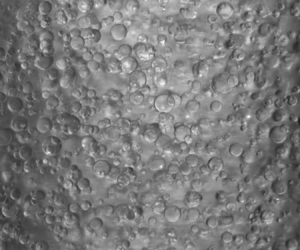
Figure 1. (a) A sketch of the experimental set-up. The gap between the outer and inner cylinders is filled with the emulsion. The inner cylinder is connected to a rheometer so that the torque of the inner cylinder is directly measured by the torque sensor of the rheometer. A high-speed camera is used to capture the dispersed oil droplets. (b) Typical snapshots of the emulsion for various  $Re$ at a given oil volume fraction
  $\phi =1\,\%$. From left to right are the cases of
  $Re=7.81\times 10^{3}$,
  $1.04\times 10^{4}$ and
  $2.08\times 10^{4}$. All three cases are recorded with a high-speed camera connected with a long-distance microscope.
3. Results and discussion
3.1. Statistical properties of droplets at a low volume fraction
The size distribution of dispersed droplets is an important statistical parameter, as it characterizes the microscopic structure of the turbulent emulsion, which closely links to the macroscopic rheological properties and the global transport properties of the fluid system. At a low volume fraction, the droplet sizes in the turbulent emulsion eventually show a statistically stationary distribution for the current experiments under stationary stirring conditions.
Figure 1(b) shows some typical snapshots of the emulsion for three different Reynolds numbers  $Re=\omega _{i}r_id/\nu$. Since in these cases the volume fraction of the oil phase is very low (
 $\phi =1\,\%$), the viscosity of the emulsion is approximately equal to that of the continuous phase, i.e.
  $\nu =\nu _{w}$. It is expected that the average droplet size of the emulsion at a higher
  $Re$ will be smaller than that at a lower
  $Re$. The reason is that the higher average shear strength, in the cases of larger
  $Re$, promotes the breakup of oil droplets.
Droplet interfaces are extracted from the recorded images, at various Reynolds numbers, and the diameter of all the detected droplets is calculated and normalized with the average droplet diameter, for each  $Re$ case, as
  $X = D/\left \langle D\right \rangle$. The distribution of the number of droplets of size
  $X$, as a function of
  $X$, is computed as the probability density function (PDF) of the droplet size and shown in figure 2(a), for various Reynolds numbers. It is clear (solid lines in figure 2a) that the experimental results at all Reynolds numbers can be well described with the log-normal distribution
 \begin{equation} P(X) = \frac{a}{X\sigma_0\sqrt{2{\rm \pi}}}\exp\left[-\frac{[\log(X) - \log(X_0)] ^{2}}{2\sigma_0^{2}}\right], \end{equation}
where  $a$,
$a$,  $X_0$ and
  $\sigma _0$ are fitting parameters. The deviation from the standard log-normal distribution for points in the range
  $X > 1.5$, for two cases of high
  $Re$ (
 $Re = 2.08\times 10^{4}$ and
  $2.60\times 10^{4}$), is due to the relatively fewer statistics for large droplet size. These log-normal distributions suggest that fragmentation is the primary process for droplet generation in the current system. Similar fragmentation processes are also observed in other systems (Villermaux Reference Villermaux2007), including plume formation in Rayleigh–Bénard turbulence (Zhou, Sun & Xia Reference Zhou, Sun and Xia2007; Bosbach, Weiss & Ahlers Reference Bosbach, Weiss and Ahlers2012) among others. In addition, it is found that the fitted value of the standard deviation
  $\sigma _0$ decreases monotonically with increasing
  $Re$ (see the inset of figure 2a). This means that the distribution of droplet size becomes narrower at higher
  $Re$, as clearly shown in figure 2(a). Some additional analyses of the distribution of droplet size are provided in appendix C using the gamma distribution function, which is found to be a good description of the droplet breakup during the atomization process (Villermaux Reference Villermaux2007). The next question is what sets the droplet size in the typical size in the fragmentation process leading to droplet formation.

Figure 2. (a) The PDF of the droplet diameter, with respect to the average diameter, for various Reynolds numbers,  $Re$. The solid lines denote the fitting results with a log-normal distribution function. The statistics are based on
  ${O}(10^{3})$ droplet samples for each
  $Re$ value. The statistical error bars are shown for all
  $Re$ cases. The fitted values of the standard deviation
  $\sigma _{0}$ as a function of
  $Re$ are shown in the inset. (b) The average droplet diameter normalized by the gap width as a function of the Reynolds number. The blue circles are the data of the droplet diameter for
  $\phi =1\,\%$ measured in experiments, and the error bars are based on the errors of the edge detection. The red solid line denotes the power-law dependence based on the Hinze relation using the local energy dissipation rate in the bulk (3.2). The black dashed line represents the weighted fit of the experimental data, the weight being based on the relative error of each data point.
In 1955, Hinze proposed that the maximum stable droplet diameter in a homogeneous and isotropic turbulent flow is given by  $D = C(\rho _w/\gamma )^{-3/5}\varepsilon ^{-2/5}$, where
  $\rho _w$ is the density of the continuous phase (the ethanol–water solution in the present case),
  $\gamma$ is the surface tension between the two phases,
  $\varepsilon$ is the energy dissipation rate and the coefficient
  $C = 0.725$ was obtained by Hinze through fitting with experimental data available at that time (Hinze Reference Hinze1955). The argument of Hinze applies to a dilute distribution of droplets that occasionally coalesce due to collisions and break up due to turbulent stresses. A key element of Hinze's argument consists of assuming that droplets do not produce a significant feedback on the turbulent flow, whose statistics are those of homogeneous and isotropic turbulence. Many studies show that the average droplet size and the maximum size are proportional in turbulent emulsions (Lemenand et al. Reference Lemenand, Della Valle, Zellouf and Peerhossaini2003; Boxall et al. Reference Boxall, Koh, Sloan, Sum and Wu2012). Considering that the maximum droplet diameter in turbulent emulsions is usually unstable due to breakup and occasional coalescence, the average droplet diameter can be used as an indicator of the droplet size in the Hinze relation (Perlekar et al. Reference Perlekar, Biferale, Sbragaglia, Srivastava and Toschi2012).
We notice that the distribution of the energy dissipation rate in Taylor–Couette turbulence is inhomogeneous, i.e. the dissipation in the bulk is much smaller than that in the boundary layers. As the volume of the bulk is much larger than that of the boundary layers in the current parameter regime (Grossmann, Lohse & Sun Reference Grossmann, Lohse and Sun2016), droplets are expected to mainly distribute in the bulk, where the flow is found to be nearly homogeneous and isotropic (Ezeta et al. Reference Ezeta, Huisman, Sun and Lohse2018). The local energy dissipation rate in the bulk can be expressed as  $\varepsilon _l\sim u_{_T}^{3}/\ell$, where
  $u_{T}$ and
  $\ell$ denote the typical velocity fluctuation and the characteristic length scale of the flow. The typical velocity fluctuation
  $u_{T}$ can be approximated as
  $A\omega _{i}r_{i}$ in the current Taylor–Couette turbulent flow (van Gils et al. Reference van Gils, Huisman, Grossmann, Sun and Lohse2012) with an almost constant prefactor
  $A$ (order of 0.1). As we know that the Reynolds number can be expressed as
  $Re=\omega _{i}r_{i}d/\nu$, then the typical velocity fluctuation can be expressed as
  $u_T \sim \omega _{i}r_{i} \sim Re\cdot \nu /d$. Substituting this velocity estimation into the expression for the energy dissipation above, we obtain
  $\varepsilon _l \sim u_{T}^{3}/\ell \sim Re^{3}\nu ^{3}/d^{4}$ by assuming
  $\ell \sim d$, and this scaling dependence is also in good agreement with the recent measurement of the local energy dissipation rate in the bulk of Taylor–Couette turbulence (Ezeta et al. Reference Ezeta, Huisman, Sun and Lohse2018). Inserting this local energy dissipation expression into Hinze's relation, one obtains
 \begin{equation} \left\langle D\right\rangle/d \sim C/d\left(\frac{\rho_w}{\gamma}\right)^{{-}3/5}\varepsilon_l^{{-}2/5} \sim Re^{{-}6/5}, \end{equation}
suggesting that the average droplet diameter has a power-law dependence on  $Re$ with an effective power-law exponent of
  $-$1.20 (equation (3.2)). We compare the dependence of the normalized droplet size on
  $Re$ from the experiments and the model in figure 2(b). The best fit of the experimental data gives a scaling exponent of
  $-1.18 \pm 0.05$. We find that the scaling dependence based on the local energy dissipation rate in the bulk (red solid line) agrees well with the experimental data. The results show that the scaling dependence of the droplet size on
  $Re$ could be connected to turbulent fluctuations in the bulk of the system. The discussion above is a simple analysis based on the scaling law. A more in-depth and quantitative understanding of the droplet formation in a turbulent (Taylor–Couette) emulsion flow deserves further studies in the future.
3.2. Effective viscosity and shear-thinning effects
The torque of the inner cylinder is directly measured by the rheometer sensor for different oil volume fractions,  $\phi$, and angular velocities,
  $\omega _{i}$, as depicted in figure 3(a), which shows that the faster the inner cylinder rotates, the larger is the torque needed to maintain the selected angular velocity. The torque becomes larger when the oil volume fraction is increased at a given angular velocity, indicating that the oil additive will bring an obvious change to the rheological property of the emulsion system. Combined with the flow properties of Taylor–Couette turbulence at various Reynolds numbers (van Gils et al. Reference van Gils, Bruggert, Lathrop, Sun and Lohse2011a,Reference Van Gils, Huisman, Bruggert, Sun and Lohseb; Huisman et al. Reference Huisman, Van Der Veen, Sun and Lohse2014; Ostilla-Mónico et al. Reference Ostilla-Mónico, Van Der Poel, Verzicco, Grossmann and Lohse2014; Grossmann et al. Reference Grossmann, Lohse and Sun2016), we can calculate the effective viscosity of emulsions in these dynamical equilibrium states. We use the same method as that recently proposed for viscosity measurements in a very high-Reynolds-number Taylor–Couette flow (Bakhuis et al. Reference Bakhuis, Ezeta, Bullen, Marin, Lohse, Sun and Huisman2020).

Figure 3. (a) Torque measurements. The torque that is required to maintain the inner cylinder at a constant angular velocity,  $\omega _{i}$, is measured for the emulsion systems with oil volume fractions corresponding to
  $\phi =0\,\%$, 1 %, 5 %, 10 %, 20 %, 30 % and
  $40\,\%$. As an estimate for the error on the torque measurements, we use the standard deviation and find that it is smaller than
  $0.8\,\%$ for all volume fractions (see appendix A for details). The error results are therefore smaller than the symbol size. (b) The dependence between the dimensionless torque,
  $G$, and the Reynolds number,
  $Re$, using the effective viscosity. All these sets of data at the various oil volume fractions collapse into a master curve, and the error is less than
  $1\,\%$. The inset shows the dimensionless torque compensated with
  $Re^{-1.58}$.
An effective power-law dependence between  $G$ and
  $Re$ can be obtained as
  $G \propto Re^{\beta }$ for the Taylor–Couette turbulent flow, and the power-law exponent
  $\beta$ depends on the Reynolds number regime (Grossmann et al. Reference Grossmann, Lohse and Sun2016). Here we assume that the power-law dependence
  $G \propto Re^{\beta }$ can still be applied to the two immiscible liquids in our Taylor–Couette turbulent flow. As a reference case, this relation can be determined by using the results of the pure ethanol–water mixture (
 $\phi =0\,\%$) with a known viscosity. When we plot together all data for the various oil fractions in a
  $G$–
$G$– $Re$ plot, and collapse them on a master curve with an effective exponent of
  $\beta = 1.58$ (figure 3b), the effective viscosity is a fitting parameter for each case. To demonstrate the quality of the overlap of the different data sets, all data are compensated by
  $Re^{1.58}$ (inset of figure 3b), which clearly shows that the effective power-law dependence works very well. Remarkably, the power-law dependence
  $G \propto Re^{1.58}$ for single-phase Taylor–Couette flows still works well for the present two-phase emulsion flows. By using the effective power-law exponent of
  $\beta = 1.58$ between
  $G$ and
  $Re$, we can calculate the effective viscosity of the emulsion at various
  $\omega _{i}$ and
  $\phi$ with an expression of
  $\nu _{eff}=\nu _{w}(\tau /\tau _{w})^{2.38}$; here
  $\nu _{w}$,
  $\tau _{w}$ and
  $\tau$ denote the viscosity of the ethanol–water solution and the measured torques of the ethanol–water solution and the emulsion, respectively. It should be noted that
  $\nu _{w}$ is known, but
  $\nu _{eff}$,
  $\tau _{w}$ and
  $\tau$ are dependent on the experimental settings, i.e.
  $\phi$ and
  $\omega _{i}$. The detailed calculation of the effective viscosity is documented in appendix B.
To understand the effect of oil addition on the rheology of the emulsion in turbulent shear flows, we systematically vary two parameters of the system, i.e. the oil volume fraction,  $\phi$, and the angular velocity of the inner cylinder,
  $\omega _{i}$. The effective viscosity of emulsions, as a function of
  $\phi$ and for various
  $\omega _{i}$, is reported in figure 4(a), where all data are normalized by the viscosity of the ethanol–water solution,
  $\nu _{w}$. Obviously, the effective viscosity of the emulsion increases with increasing oil volume fraction,
  $\phi$, for all
  $\omega _{i}$ cases. While the effective viscosity has a weak dependence on
  $\phi$ in the dilute regime (e.g. for
  $\phi <5\,\%$), it displays a stronger dependence for larger
  $\phi$. The hydrodynamic or contact interactions between oil droplets for larger
  $\phi$ are expected to yield an increasing viscous contribution, somehow similar to what is observed for the case of dispersions of hard spheres in suspensions (Guazzelli & Pouliquen Reference Guazzelli and Pouliquen2018). The relation between the effective viscosity and the volume fraction of dispersed solid particles in particle–fluid suspensions is also plotted in figure 4(a) for comparison. Strictly speaking, we find that the effective viscosities of the emulsions, at all
  $\omega _{i}$, are smaller than that of the dependence proposed by Krieger & Dougherty (Reference Krieger and Dougherty1959). Here it needs to be emphasized that this model was developed for suspensions of monodispersed hard spheres in fluids in the viscous regime. This disagreement in the viscosity can be due to the different nature of the dispersed phases: the dispersed solid particles have a fixed, undeformable shape, while the dispersed oil droplets can deform; the solid particles have a fixed size, while the droplets can dynamically coalesce and break up under the flow. The dynamics of the dispersed droplets in emulsions is therefore much richer than that of the solid particles in suspensions.

Figure 4. (a) The effective viscosity normalized by the viscosity of the ethanol–water mixture,  $\nu _{eff}/\nu _{w}$, as a function of the volume fraction of the dispersed oil phase
  $\phi$ at various angular velocity
  $\omega _{i}$. The solid line denotes the effective viscosity model for solid particle suspensions of Krieger & Dougherty (Reference Krieger and Dougherty1959). The calculation of the effective viscosity is based on the torque measurements. The relative standard deviation is less than
  $2.5\,\%$, so the errors bars are smaller than the symbol size. (b) The effective viscosity of the emulsion versus the characteristic shear rate
  $\dot {\gamma }$ of the flow. The data for the different oil volume fractions,
  $\phi$, are denoted by the open symbols with various colours in the legend. The solid lines show the fitting results (fits 1–7) using the Herschel–Bulkley model (Herschel & Bulkley Reference Herschel and Bulkley1926) for various volume fractions. The inset shows the power-law index
  $n$ as a function of the volume fraction
  $\phi$.
Furthermore, the effective viscosity is found to decrease with increasing  $\omega _{i}$ for a given
  $\phi$ as indicated in figure 4(a). In other words, the turbulent emulsion shows a continued shear-thinning behaviour. To reveal this effect better, we plot the effective viscosity as a function of shear rate in figure 4(b), where the shear rate is defined as
  $\dot {\gamma }=\omega _{i}r_{i}/d$. Though the Taylor–Couette flow is not a planar shear flow, the shear rate
  $\dot {\gamma }$ can still represent well the effective shear strength of the system. When the volume fraction of oil is
  $\phi =0\,\%$ (i.e. pure ethanol–water), the system is a single-phase flow state and, as expected, the effective viscosity does not change with the shear rate
  $\dot {\gamma }$. With the addition of the oil phase, the effective viscosity of the emulsion decreases with increasing
  $\dot {\gamma }$, and this effect is more pronounced for high volume fractions, as shown in figure 4(b). This shear-thinning behaviour is similar to what was found in a suspension of deformable microgel particles under steady shear flow (Adams et al. Reference Adams, Frith and Stokes2004).
To quantify the shear-thinning effect of the turbulent emulsion, we compare our data with the Herschel–Bulkley model (Herschel & Bulkley Reference Herschel and Bulkley1926):
 \begin{equation} \mu_{eff}=k_{0}\dot{\gamma}^{n-1}+\tau_{0}\dot{\gamma}^{{-}1}, \end{equation}
where  $\mu _{eff}$ is the effective dynamic viscosity,
  $k_{0}$ and
  $n$ represent the consistency and the flow index, respectively, and
  $\tau _{0}$ is the yield shear stress. As the system is far from the jamming state, the yield shear stress is expected to be zero in the current case (
 $\tau _{0}=0$). Consequently, the Herschel–Bulkley model can then be simplified as
  $\nu _{eff}/\nu _{w}=K\dot {\gamma }^{n-1}$. The fitting results using the Herschel–Bulkley model for various volume fractions are also shown in figure 4(b). As expected, the flow index is around 1 at very low volume fractions, suggesting that the fluid behaves like a Newtonian fluid. The flow index,
  $n$, monotonically decreases with increasing volume fraction of dispersed phase (inset of figure 4b), indicating a more pronounced shear-thinning effect for the emulsions with high oil volume fractions. The agreement between the experimental data and the Herschel–Bulkley model indicates that the shear-thinning effect can be well described by this classical non-Newtonian model, opening an important avenue for the description of the effective viscosity of turbulent emulsion systems.
4. Conclusions
Turbulent emulsions are complex physical systems coupling macro- and micro-scales. In this work, we investigated the dynamics of emulsions of oil droplets dispersed in an ethanol–water solution without surfactant additive in a turbulent shear flow. Firstly, we find that the PDF of the droplet sizes follows a log-normal distribution, suggesting a fragmentation process in the droplet generation process. By comparing the droplet size for various Reynolds numbers for the system at a low volume fraction of  $1\,\%$ with Hinze theory, we find that the scaling dependence of the droplet size on Reynolds number can be connected to the turbulent fluctuations in the bulk of the system.
The effective viscosity of the emulsion is found to increase with increasing oil volume fraction, but the increasing trend is weaker than that reported for solid particle suspensions. This difference is associated with the different nature (deformability and size distribution) of the dispersed phase in fluid–fluid emulsions. Additionally, we find that the effective viscosity of the emulsions decreases with increasing shear rate, displaying a shear-thinning behaviour that can be quantitatively described using the classical Herschel–Bulkley model via a dependency of the flow index on the volume fraction. The shear-thinning effect of a turbulent emulsion has many potential applications, such as drag reduction of multicomponent liquid systems in turbulent states. The current findings have important implications for extending the knowledge on turbulence and low-Reynolds-number emulsion flows to turbulent emulsion flows.
Acknowledgements
We thank F. Risso, D. Lohse, S. Huisman and T. van Vuren for insightful suggestions and discussions, and thank H. Duan, P. Lyu, B. Xu and Y. Xiang for help with the experimental set-up.
Funding
This work is financially supported by the Natural Science Foundation of China under grant nos. 11988102, 11861131005, 91852202 and 11672156 and by the Tsinghua University Initiative Scientific Research Program (20193080058).
Declaration of interests
The authors report no conflict of interest.
Appendix A. Experiments
A.1. Liquids used in the current study
We use silicone oil (dispersed phase) and ethanol–water mixture (continuous phase) in the experiments. The silicone oil and ethanol–water solution are immiscible. The density of the silicone oil (type Shin-Etsu KF-96L-2cSt) is  $\rho _{o}=866\ \textrm {kg}\ \textrm {m}^{-3}$. We use an aqueous mixture of deionized water and ethanol as the second liquid. The volume fraction of water is
  $25\,\%$. The density of the ethanol–water mixture is
  $\rho _{w}=860\ \textrm {kg}\ \textrm {m}^{-3}$, which is very close to that of the silicone oil. The density match of these two kinds of liquids can eliminate the effect of centrifugal force on liquid distribution. Both ethanol–water mixture and silicone oil are transparent, which facilitates the imaging of emulsions. As the refractive indices of these two kinds of liquids are different, we can distinguish the oil droplets from the background of ethanol–water.
The viscosity is measured using a hybrid rheometer of type TA DHR-1 (Discovery Hybrid Rheometer, TA Instruments). We equip the rheometer with a parallel plate, which is appropriate for measurements of low-viscosity liquids in the current study. The Peltier steel plate under the measured liquids provides temperature control and measurement with an accuracy of  ${\pm }0.1\,^{\circ }\textrm {C}$. Plots of kinematic viscosity
  $\nu$ versus temperature
  $T$ for these two kinds of liquids are shown in figure 5. The viscosity of ethanol–water is larger than that of silicone oil in the measured temperature range of
  $10$ to
  $30\,^{\circ }\textrm {C}$. At the experimental temperature,
  $T=22\,^{\circ }\textrm {C}$, we found the viscosity of ethanol–water is
  $\nu _{w}=2.4\times 10^{-6}\ \textrm {m}^{2}\ \textrm {s}^{-1}$, which is close to that of silicone oil of
  $\nu _{o}=2.1\times 10^{-6}\ \textrm {m}^{2}\ \textrm {s}^{-1}$. The interfacial tension between the dispersed phase and continuous phase is an important parameter in emulsions, which is closely linked to the breakup and coalescence of droplets. We measure the interfacial tension between the two kinds of liquids (ethanol–water and silicone oil) used in the current experiments with the pendant drop method. The type of measurement instrument is an SCA20. The interfacial tension is calculated using characteristic parameters of the drop profiles and density difference of the liquids. We perform six measurements and use the average value as the final result of interfacial tension:
  $\gamma =4.53\ \textrm {mN}\ \textrm {m}^{-1}$. All measurements are conducted at a temperature of
  $T=22\,^{\circ }\textrm {C}$.

Figure 5. The kinematic viscosity  $\nu$ as a function of temperature
  $T$. The red circles denote measured viscosity of ethanol–water and the blue circles denote that of silicone oil. For the temperature of experiments,
  $T=22\,^{\circ }\textrm {C}$, the viscosity of ethanol–water is
  $\nu _{w}=2.4\times 10^{-6}\ \textrm {m}^{2}\ \textrm {s}^{-1}$ while that of silicone oil is
  $\nu _{o}=2.1\times 10^{-6}\ \textrm {m}^{2}\ \textrm {s}^{-1}$.
A.2. Torque measurement
The torque is a response parameter of the emulsion system in the current study. The torque is directly measured by the rheometer through a shaft connected to the inner rotating cylinder with high accuracy of up to  $0.1\ \textrm {nN}\ \textrm {m}$. For each experiment, we set the angular velocity
  $\omega _{i}$ of the inner cylinder as a constant value. After the system reaches a statistically stable state, direct measurements of time series of torque are recorded. A typical time series of torque measurements is shown in figure 6. The standard deviation of the torque time series is
  $15.47 \ \mathrm {\mu }\textrm {N}\ \textrm {m}$, which is much smaller than the torque value and consequently fulfils the requirement of the torque measurement. To show the quality of torque measurements, we calculate the relative standard deviation (RSD) for all cases in the current study, as shown in figure 7. We find that all values of RSD are smaller than
  $0.8\,\%$, indicating that the torque measurements are reliable. The results show that the RSD does not change with oil volume fraction
  $\phi$ and angular velocity
  $\omega _{i}$.

Figure 6. A typical result of time series of torque measurements for the emulsion system. The oil volume fraction is  $\phi =1\,\%$ and the Reynolds number is
  $Re=5.21\times 10^{3}$ in this case. The standard deviation of the torque time series is
  $15.47 \ \mathrm {\mu }\textrm {N}\ \textrm {m}$, which is much smaller than the averaged torque value.

Figure 7. (a) The RSD of torque time series as a function of volume fraction for various angular velocities. (b) The RSD of torque time series as a function of angular velocity for various volume fractions.
A.3. Imaging of the dispersed drops
The statistical properties of dispersed oil droplets in emulsions are important parameters in the current study. We use a high-speed camera to capture the drops, which are constantly moving rapidly along with the flow in turbulent states. Two sets of camera lenses are used. One is a Nikon 105 mm f/2.8G macro lens with an extension tube that gives about  $2\times$ magnification ratio (Set 1). This set of lenses is used for a low-
 $Re$ case (
 $Re = 5.21 \times 10^{3}$), in which the drop size is in the range of about
  $40\text {--}500\ \mathrm {\mu }\textrm {m}$. The light source is two front lamps, and the reflected light from the surface of the inner cylinder is used for imaging. For the experiments at higher
  $Re$ (
 $Re>5.21\times 10^{3}$), another set of NAVITAR microscopic lenses coupled with a
  $5\times$ objective type (Mitutoyo M Plan Apo) is connected to the high-speed camera to resolve the very small oil droplets in turbulent Taylor–Couette flows (Set 2). For this set of lenses, the light source is coaxial with the microscope so that we can obtain a better view in the small observation area. The axes of the lenses are at about half the height of the system so that we can reduce the edge effects from top and bottom.
To reduce the effect of curvature, both these two sets of lenses are focused on the central area of the Taylor–Couette system. For both sets of lenses, we perform a length calibration before experiments. The typical results of length calibration are shown in figure 8. The length of the images is 600 pixels and the height is 400 pixels. Figures 8(a) and 8(c) show the calibration images for Set 1 and Set 2, respectively. Each of the smallest tick intervals is  $100\ {\mathrm {\mu }}\textrm {m}$. We plot the pixel distance as a function of the tick distance in figure 8(b,d). The linearity of the data indicates that the effect of curvature can be safely neglected in the current measurements.

Figure 8. The results of length calibration for two sets of lenses used in the current study. (a) The image of length calibration for Set 1. Each of the smallest tick intervals is  $100\ \mathrm {\mu }\textrm {m}$. (b) The calibration results of Set 1. The
  $x$ axis corresponds to the ticks in (a) and the
  $y$ axis corresponds to the pixel distance from the left border in (a). (c) The image of length calibration for Set 2. Each of the smallest tick intervals is
  $100\ \mathrm {\mu }\textrm {m}$. (d) The calibration results of Set 2. The
  $x$ axis corresponds to the ticks in (c) and the
  $y$ axis corresponds to the pixel distance from the left edge in (c).
Appendix B. The effective viscosity calculation
First, we calculate  $Re$ and
  $G$ at various angular velocities
  $\omega _i$ for pure ethanol–water mixture (
 $\phi =0\,\%$) with a known viscosity. When we plot these data in a
  $G$–
$G$– $Re$ plot, we find a scaling law as
  $G\sim Re^{1.58}$. Further, we can write this relation as
  $G=KRe^{1.58}$, where
  $K$ denotes a constant prefactor. If we insert the definitions of
  $G$ and
  $Re$ to this dependence, we obtain a dependence of torque
  $\tau$ and viscosity
  $\nu$ as
 \begin{equation} \tau=AK\nu^{0.42}, \end{equation}
where  $A$ is equal to
  $2{\rm \pi} L\rho /(\omega _{i}r_id)^{0.42}$. We assume that this relation is still valid for emulsion systems with various oil volume fractions and Reynolds numbers. We write the torque and effective viscosity of the emulsion system as
  $\tau$ and
  $\nu _{eff}$ for a constant angular velocity
  $\omega _i$ at a volume fraction of
  $\phi$. For the pure ethanol–water mixture (
 $\phi =0\,\%$) system at the same angular velocity, we obtain the measured torque value
  $\tau _{w}$ and the viscosity
  $\nu _{w}$. Based on our assumption, these two systems both follow the relation given above. Because the angular velocities of these two systems are the same, the prefactor
  $A$ is therefore also the same. Then, we can derive the following relation:
 \begin{equation} \frac{\nu_{eff}}{\nu_{w}}=\left(\frac{\tau}{\tau_{w}}\right)^{2.38}. \end{equation}
The effective viscosity of emulsion systems  $\nu _{eff}$ can be obtained based on this relation. To further verify our assumption above, we calculate
  $G$ and
  $Re$ for various volume fractions and angular velocities using the effective viscosity obtained for each case. When we plot together all data of various oil fractions in a
  $G$–
$G$– $Re$ plot, we find that all data of
  $G$ versus Re collapse into a master curve. The fitting results for the oil fractions of
  $\phi =1\,\%$, 5 %, 10 %, 20 %, 30 % and 40 % show that all these six sets of data follow the relation
  $G=KRe^{1.58}$ with an error bar of only
  $1\,\%$, which strongly supports the assumption above. Here we provide a new approach for the measurement of the effective viscosity of emulsions in high-Reynolds-number turbulent states.
Appendix C. The analysis of droplet size
C.1. Image processing
The videos and images obtained in the experiments are analysed using the Matlab code and ImageJ software. For better post-processing, the original images are firstly cropped and exported as tiff-format images. The size of the clipping window is  $300\ \textrm {pixels} \times 1024\ \textrm {pixels}$. At the same time, we determine the interval between every two frames based on the average speed of the droplets moving in the horizontal direction, so that the oil droplets in each image are not counted repeatedly.
Next, we adjust the contrast of images and detect the boundary of drops using the Matlab code. The radii of droplets are exported as the data sets for further processing. Typical results of boundary detection for the various Reynolds numbers are shown in figure 9. Most of the oil droplets in the images are well captured. A few drops are not detected, because they are out of the focal plane, inducing boundaries that are too indistinct. Considering that we count enough droplet samples ( ${O}(10^{3}$)), these undetected drops do not have much influence on the analysis of the statistical characteristics for the drops.

Figure 9. The results of drop detection for various Reynolds numbers: (a)  $Re=7.81\times 10^{3}$, (b)
  $Re=1.04\times 10^{4}$ and (c)
  $Re=1.56\times 10^{4}$. The volume fraction of oil is
  $\phi =1\,\%$. The blue circles are the boundaries of the oil drops from edge detection. Most of the drops in the images are captured with a high fidelity.
In order to verify the reliability of drop detection using the Matlab code, we also use another method to calculate the droplet size. We use ImageJ software to obtain the diameter of droplets by manually counting the pixel distance. A comparison between the results obtained using manual counting and those using the Matlab code is shown in figure 10. The differences between the two methods are very small, and both sets of results are in good agreement with the Hinze relation (Hinze Reference Hinze1955), indicating that the results obtained using both the Matlab code and manual counting are reliable. The numbers of detected droplet samples at various  $Re$ using the Matlab code and manual counting are shown in table 1. Of course, detection using the Matlab code provides more statistics, and we therefore use the results from the Matlab detection for all cases in the main paper.

Figure 10. A comparison between the results of the average drop diameter determined using the Matlab code and that by manually counting pixels in ImageJ software. The blue circles denote the data determined using the Matlab code and the red triangles denote the results from the manual pixel counting. The solid black line is the fitted power-law dependence based on the Hinze relation (Hinze Reference Hinze1955). All data are obtained for an oil volume fraction of  $\phi =1\,\%$.
Table 1. The numbers of detected droplet samples at various  $Re$ using the Matlab code and manual counting.

C.2. The distribution of droplet size
The distribution behaviours of droplet sizes in emulsions are found to be well described by log-normal distribution functions. We have fitted the same data using the gamma distribution function:
 \begin{equation} P(X = D/\langle D \rangle) = \frac{n^{n}}{\varGamma(n)}X^{n-1}\,\textrm{e}^{{-}nX}, \end{equation}
where  $n$ is a constant and
  $\varGamma (n)$ is the gamma function. This function is expected to be a good description of droplet size during atomization (Bremond & Villermaux Reference Bremond and Villermaux2006; Villermaux Reference Villermaux2007). The results of the fit are shown in figure 11. It is found that the gamma distribution function can also describe the droplet size distribution for most
  $Re$ cases. In addition, we also see a monotonic increase of the index
  $n$ with increasing
  $Re$, indicating that the distribution is narrowed. Indeed, we cannot tell which distribution function is better for describing the distribution of the droplet size for all cases, given the current data. Thus, while we report only the results for the log-normal distribution in the main text, the results for gamma distribution are also provided here for the purpose of comparison. The distribution of droplet size will be studied in the future.

Figure 11. The PDF, in log–log scale, of the droplet size for various Reynolds numbers,  $Re$. The solid lines denote the fitted results using gamma distribution functions. The inset shows the fitted value of the index
  $n$ as a function of
  $Re$.
$Re$.


