3.1. Instantaneous flow field and skin friction coefficients

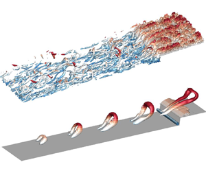
Figures 4(a) and 4(b) plot the isosurface of reverse flow ($u<0$) in a typical instantaneous flow field near the FFS, which is also shown in a supplementary animation. In general, the reverse flows occur in irregular shaped volumes upstream and downstream of the leading edge of the step. The volume of reverse flow upstream of the step can extend across the entire height of the step. This is in line with the spillover of the separation bubble upstream of the FFS observed by Stüer et al. (Reference Stüer, Gyr and Kinzelbach1999), Wilhelm et al. (Reference Wilhelm, Härtel and Kleiser2003) and Pearson et al. (Reference Pearson, Goulart and Ganapathisubramani2013). The extremely high elevation of reverse flows upstream of the step occurs quasi-periodically in the spanwise direction. It is also interesting to note that over the FFS, reverse flow disappears in patches (marked using arrows and circles in figures 4(a) and 4(b), respectively). The $x$–$y$ planes across these intermediate reattachment patches would exhibit dual separation bubbles over the step, which is reminiscent of the break-up event of the separation bubble over a forward-backward-facing step observed by Fang & Tachie (Reference Fang and Tachie2019b). From the supplementary animation, the spillover of the separation bubble upstream of the step tends to occur near the same spanwise location as the intermediate reattachment over the step.

Figure 4. Characterization of a typical instantaneous flow field. (a) Isosurface of the reverse flow ($u<0$) near the step. The thick arrows mark intermediate reattachment regions over the step. (b) Top view of (a). The black circles mark the same regions indicated using arrows in (a). (c) Isosurface of swirling strength $\lambda _{ci}h/U_C=10$. (d) Superposition of the isosurfaces of the reverse flow and $\lambda _{ci}h/U_C=10$. Note that (a,b) and (c,d) use different contour levels of $y$ to highlight different features. (e) Contour of spanwise skin friction coefficient $C_{f3}$ superimposed with the skin friction vectors ($C_{f3}$, $C_{f2}$). Not all vectors are plotted for clarity. An animation is also shown in a supplementary movie 1 available at https://doi.org/10.1017/jfm.2021.395.

Figures 4(c) and 4(d) show the vortical structures identified by the isosurface of $\lambda _{ci}$, which is defined as the imaginary part of the eigenvalues of the velocity gradient tensor (Zhou et al. Reference Zhou, Adrian, Balachandar and Kendall1999). From figure 4(c), the density of vortical structures suddenly increases as the step is approached, and the vortical structures leaning over the step are preferentially aligned in the streamwise-vertical planes. Downstream of the leading edge of the FFS, spanwise orientated vortical structures begin to appear, and eventually a ‘forest’ of hairpin-like structures appear. It is evident in figures 4(d) that the vortical structures leaning over the FFS coincide with the spillover of reverse flow upstream of the FFS.

Figure 4(e) plots the instantaneous skin friction coefficient over the frontal surface of the step. In the present paper, the instantaneous skin friction coefficient in the $x_i$ direction is defined as $C_{fi}=\nu ({\partial u_i}/{\partial n})|_{wall} / (U_C^2/2)$, where $n$ denotes the wall normal direction. Note that in this paper, $C_{fi}$ represents the instantaneous skin friction coefficient instead of the associated mean value as commonly used in the literature. It is evident in figure 4(e) that pairs of positive and negative $C_{f3}$ occur, and the skin friction vectors ($C_{f3},C_{f2}$) exhibit a pattern of alternating saddle and nodal points in the spanwise direction. This observation is similar to the oil-film visualization on the frontal surface of forward-backward-facing steps submerged in a turbulent channel flow by Martinuzzi & Tropea (Reference Martinuzzi and Tropea1993). In accordance with figures 4(b) and 4(e), the spillover of reverse flow upstream of the step appears to be near the centre of each pair of positive and negative $C_{f3}$ on the frontal surface of the step.

In view of the well-organized alternating positive and negative $C_{f3}$ on the frontal surface of the step shown in figure 4(e), it is worthwhile further investigating the statistical properties of the skin friction coefficients near the step. While the mean ($\overline {C_{f1}}$) and root-mean-square ($C_{f1, rms}'$) values of streamwise skin friction induced by sharp-edged bluff bodies have been examined in the literature (e.g. Dianat & Castro Reference Dianat and Castro1984; Hattori & Nagano Reference Hattori and Nagano2010), the corresponding spanwise skin friction has not been reported. Figure 5 presents the mean and root-mean-square values of all applicable skin friction coefficients on the bottom wall upstream of the step as well as the frontal and top surfaces of the step. From figure 5(a), $\overline {C_{f1}}$ has three local minima: one near the mean recirculation core in the upstream corner of the step, one immediately downstream of the leading edge and one near the core of the mean recirculation bubble over the step, which pattern is similar to that observed by Hattori & Nagano (Reference Hattori and Nagano2010). The magnitudes of $C'_{f1,rms}$ and $C'_{f3,rms}$ are close to each other upstream of the step ($x/h<0$), while the latter becomes slightly larger than the former for $x/h>1.0$. The comparable peak values of $C'_{f1,rms}$ and $C'_{f3,rms}$ suggest that the spanwise fluctuating flow motion can be as dynamically significant as the streamwise counterpart. Furthermore, as seen in figure 5(b), $C'_{f3,rms}$ is significantly larger than $C'_{f2,rms}$ on the frontal surface of the step. In fact, $C'_{f3,rms}$ monotonically increases in the vertical direction and the peak value (at the leading edge of the step) is more than twice the maximum value of $C'_{f1,rms}$. The high levels of $C'_{f3,rms}$ on the frontal surface of the step indicate that the alternating positive and negative $C_{f3}$ observed in figure 4(e) represents a strong and coherent flow structure at play.

Figure 5. (a) Streamwise variation of $\overline {C_{f1}}$, $C'_{f1,rms}$ and $C'_{f3,rms}$ over the bottom wall and top surface of the step. The vertical dash-dot-dotted line marks the mean reattachment point. (b) Vertical variation of $\overline {C_{f2}}$, $C'_{f2,rms}$ and $C'_{f3,rms}$ on the frontal surface of the step.

3.2. Turbulence statistics

Figure 6(a) shows the contour of streamwise mean velocity ($\bar {u}$) and mean streamlines near the FFS. Two distinct mean separation bubbles occur upstream of and over the step. Upstream of the step, the mean separating point on the bottom wall is at $x/h=-2.0$, while the stagnation point on the frontal surface is at $y/h=0.6$. These locations agree well with the separating point ($x/h\in [-1.73,-1.93]$) and stagnation point ($y/h\in [0.59,0.61]$) observed by the DNS study of Hattori & Nagano (Reference Hattori and Nagano2010) for an FFS submerged in an oncoming TBL, but are different than those reported in experimental and large-eddy simulation studies of FFS flows (Moss & Baker Reference Moss and Baker1980; Addad et al. Reference Addad, Laurence, Talotte and Jacob2003; Graziani et al. Reference Graziani, Kerhervé, Martinuzzi and Keirsbulck2018; Fang & Tachie Reference Fang and Tachie2020). For instance, Fang & Tachie (Reference Fang and Tachie2020) and Graziani et al. (Reference Graziani, Kerhervé, Martinuzzi and Keirsbulck2018) observed that the mean separation on the bottom wall occurs at $x/h=-0.85$ and $x/h=-1.0$, respectively, while the mean stagnation point on the frontal surface is at $y/h=0.45$ and $y/h=0.55$, respectively. It is also observed in figure 6(a) that the mean reattachment length over the step is $1.72h$. This value is comparable to 1.82–1.86$h$ and $1.6h$ reported by Hattori & Nagano (Reference Hattori and Nagano2010) and Fang & Tachie (Reference Fang and Tachie2020), respectively, but significantly smaller than that ($3.2h$) observed by Graziani et al. (Reference Graziani, Kerhervé, Martinuzzi and Keirsbulck2018).

Figure 6. (a) Contour of streamwise mean velocity ($\bar {u}$) superimposed with representative mean streamlines (solid lines). The dashed isopleth is at $\bar {u}=0$. (b) Magnitudes (contour) and directions (vectors) of principal stretching superimposed with representative mean streamlines (solid lines). The dashed line is a function of $y/h=0.5\sqrt {x/h}+1.0$, and is denoted by PSL for conciseness in the present paper. Plot (c) magnifies the region in (b) near the leading edge of the step.

Following Fang & Tachie (Reference Fang and Tachie2020), the mean flow field is further investigated in terms of the topological characteristics of the mean shear, i.e. $S_{ij}=(\partial \bar {u}_i/\partial x_j + \partial \bar {u}_j/\partial x_i)/2$. In the present study, all non-zero components of $S_{ij}$, which are $S_{11}$, $S_{12}$ and $S_{22}$, are in the $x$–$y$ plane due to spanwise homogeneity, and are hereafter denoted by $\boldsymbol {S_{xy}}$ for conciseness. The eigendecomposition of $\boldsymbol {S_{xy}}$ is expressed as

(3.1)\begin{equation} \boldsymbol{S_{xy}}= \begin{bmatrix} \dfrac{\partial \bar{u}}{\partial x} & \dfrac{1}{2}\left( \dfrac{\partial \bar{u}}{\partial y}+\dfrac{\partial \bar{v}}{\partial x}\right) \\ \dfrac{1}{2}\left( \dfrac{\partial \bar{u}}{\partial y}+\dfrac{\partial \bar{v}}{\partial x}\right) & \dfrac{\partial \bar{v}}{\partial y} \end{bmatrix} = \boldsymbol{Q} \begin{bmatrix} \sigma_1 & 0 \\ 0 & \sigma_2 \\ \end{bmatrix} \boldsymbol{Q}^{\textrm{T}} . \end{equation}

Here, superscript $(\cdot )^{\textrm {T}}$ denotes the transpose of a matrix, $\sigma _1$ and $\sigma _2$ are two eigenvalues of $\boldsymbol {S_{xy}}$, and the corresponding eigenvectors are indicated by the first and second column of $\boldsymbol {Q}$, respectively. Since $\boldsymbol {S_{xy}}$ is a symmetric real matrix, its eigenvalues are real and eigenvectors are orthogonal. Due to incompressibility (equation (2.1)), $\sigma _1+\sigma _2=\text {trace}(\boldsymbol {S_{xy}})=\partial \bar {u}/\partial x+ \partial \bar {v}/\partial y=0$ holds. Without loss of generality, we define $\sigma _1$ as the positive eigenvalue of $\boldsymbol {S_{xy}}$, indicating the strength of principal stretching. Consequently, the first column of $\boldsymbol {Q}$ defines the direction of principal stretching, and is restricted to be between $-90^\circ$ and $90\,^\circ$, since $-\boldsymbol {Q}$ also defines the eigenvectors.

Figures 6(b) and 6(c) characterize the magnitudes and directions of principal stretching in the vicinity of the step. The present topology of principal stretching is similar to that observed by Fang & Tachie (Reference Fang and Tachie2020), in spite of significantly different upstream flow conditions. In the region sufficiently upstream of the leading edge (say $x/h<-1.0$ or $x/h>2.0$), the principal stretching is generally at $45^\circ$ with the streamwise direction, resembling that in a canonical TBL or fully developed channel flow. As the step is approached below the step height ($y/h<1$), principal stretching becomes steeper and eventually is aligned vertically near the frontal surface. Along the mean streamline deflected over the step, the principal stretching is approximately parallel with the mean streamline in the region slightly upstream of the leading edge of the step before becoming horizontally aligned directly above the leading edge. As evident in figure 6(c), the principal stretching switches orientation abruptly at a location given by a curved line emanating from the leading edge. This curved line fits well into the function of $y/h=0.5\sqrt {x/h}+1.0$. In Fang & Tachie (Reference Fang and Tachie2020) the principal stretching switches orientation abruptly near a straight line at $29^\circ$ with the streamwise direction. For conciseness, the dashed curve in figure 6(c) is hereafter denoted by PSL (as in ‘principal stretching line’).

Figure 7 presents the contours of all non-trivial second-order moment statistics of the fluctuating velocities and vorticities near the step. Note that, following Fang & Tachie (Reference Fang and Tachie2019b) and Fang & Tachie (Reference Fang and Tachie2020), the presented statistics in the $x$–$y$ plane are defined in the curvilinear coordinate system along the mean streamlines so as to reflect the mean streamline curvature. (Many useful counterpart flow statistics defined in the conventional Cartesian coordinate system extracted from the present DNS database have been provided in Fang, Tachie & Bergstrom (Reference Fang, Tachie and Bergstrom2021).) Specifically, the second-order moment statistics of fluctuating vorticities tangential and perpendicular to the mean streamline can be calculated as follows:

(3.2a)$$\begin{gather} (\overline{\omega_1'\omega_1'})_t = \overline{\omega_1'\omega_1'} \cos^2(\theta)+ \overline{\omega_2'\omega_2'} \sin^2(\theta)+ \overline{\omega_1'\omega_2'} \sin(2\theta), \end{gather}$$

(3.2b)$$\begin{gather}(\overline{\omega_2'\omega_2'})_t = \overline{\omega_2'\omega_2'} \cos^2(\theta)+ \overline{\omega_1'\omega_1'} \sin^2(\theta)- \overline{\omega_1'\omega_2'} \sin(2\theta), \end{gather}$$

(3.2c)$$\begin{gather}(\overline{\omega_1'\omega_2'})_t = \overline{\omega_1'\omega_2'} \cos(2\theta)- \left(\overline{\omega_1'\omega_1'}- \overline{\omega_2'\omega_2'}\right) \sin(2\theta)/2. \end{gather}$$

Figure 7. Contours of mean-square values of fluctuating velocity and vorticity along and perpendicular to the mean streamlines superimposed with mean separating streamlines (solid lines): (a) $(\overline {u'u'})_t$, (b) $(\overline {\omega _1'\omega _1'})_t$, (c) $(\overline {v'v'})_t$, (d) $(\overline {\omega _2'\omega _2'})_t$, (e) $(\overline {u'v'})_t$, (f) $(\overline {\omega _1'\omega _2'})_t$, (g) $\overline {w'w'}$ and (h) $\overline {\omega _3'\omega _3'}$. In (a,c,e,g), symbol $+$ marks the local peak upstream of the step. The dashed line represents the location of the PSL.

In the above equation, subscript $(\cdot )_t$ denotes a variable in the curvilinear coordinate system along the mean streamlines, and $\theta$ is the angle between mean velocity and the streamwise direction. The corresponding Reynolds stresses defined in the curvilinear coordinate system along the mean streamline ($(\overline {u'u'})_t$, $(\overline {v'v'})_t$ and $(\overline {u'v'})_t$) can be obtained by substituting $\omega _1'$ and $\omega _2'$ with $u'$ and $v'$, respectively, in the above equations.

As seen in figures 7(a)–7(f), these statistics show abrupt variations in a narrow area connecting the leading edge and the mean reattachment point within the mean separation bubble. This narrow area is in close vicinity of the isopleth of $\bar {u}=0$, and the associated abrupt variations of statistics are a manifestation of the abrupt variation in the orientation of the mean streamlines. Moreover, the elevated levels of the plotted statistics over the step are confined downstream of the PSL. There exists an area of elevated levels of $(\overline {v'v'})_t$ slightly upstream of the leading edge of the step. The peak value of $(\overline {v'v'})_t$ upstream of the step is much larger than that of $(\overline {u'u'})_t$ at the same location. It is therefore concluded that, in the region immediately upstream of the step, the fluctuating velocity perpendicular to the mean streamline dominates over that parallel with the mean streamline. This observation has also been made in our recent experimental study of turbulent separation induced by an FFS (Fang & Tachie Reference Fang and Tachie2020). In Fang & Tachie (Reference Fang and Tachie2020), based on the planar PIV measurement, it was speculated that the dominance of $(\overline {v'v'})_t$ upstream of the leading edge is accompanied with the dominance of fluctuating vorticity along the mean streamline. This speculation is now confirmed. Indeed, by comparing figures 7(b), 7(d) and 7(h), the dominance of fluctuating vorticity parallel to the mean streamline $(\overline {\omega _1'\omega _1'})_t$ immediately upstream of the step is apparent. It is also important to notice in figure 7 that the significant values of $(\overline {\omega _1'\omega _1'})_t$ immediately upstream of the step is also accompanied by elevated levels of $\overline {w'w'}$ in that vicinity. The upstream peak of $\overline {w'w'}$ is 50 % larger than the corresponding downstream peak, and is evidently larger than the upstream peak values of $(\overline {u'u'})_t$ and $(\overline {v'v'})_t$. It is emphasized that, to our best knowledge, the significance of the spanwise Reynolds normal stress $\overline {w'w'}$ near an FFS has not been reported before.

Figure 8 examines the streamwise variation of the vertical profiles of all three Reynolds normal stresses ($\overline {u'u'}$, $\overline {v'v'}$ and $\overline {w'w'}$). From the figure, the peak value of $\overline {w'w'}$ is larger than those of the other two Reynolds normal stresses in the region slightly upstream of the leading edge ($x/h=-0.1$), and becomes lower than the peak values of $\overline {u'u'}$ over the step. In the near-wall region (say $y/h<1.1$) over the step, $\overline {w'w'}$ dominates over $\overline {u'u'}$ and $\overline {v'v'}$ near the leading edge ($x/h=-0.1$), and becomes closes to $\overline {u'u'}$ for $x/h\geq 1.0$. On the other hand, $\overline {w'w'}$ is fairly close to $\overline {v'v'}$ in the region further away from the top surface of the step (say $y/h>1.4$). It is also noted in figure 8 that $\overline {v'v'}$ possesses two local peaks in the vertical direction at $x/h=-0.1$ and 0.1, and shows single peaks that coincide with the peak locations of $\overline {u'u'}$ in the region of $x/h\geq 1.0$. It is a common practice in experimental studies to estimate the out-of-plane Reynolds normal stress by averaging the two in-plane Reynolds normal stresses (i.e. $\overline {w'w'}\approx (\overline {u'u'}+\overline {v'v'})/2$), when only streamwise and vertical components of the velocity field are available. For example, Kim, Ji & Seong (Reference Kim, Ji and Seong2003) and Schröder et al. (Reference Schröder, Willert, Schanz, Geisler, Jahn, Gallas and Leclaire2020) used this estimation to further approximate the turbulent kinetic energy as $(\overline {u'_iu'_i})/2\approx 3(\overline {u'u'}+\overline {v'v'})/4$ for the turbulent flow separations induced by surface-mounted bluff bodies. It is evident from figure 8 that these estimations are not valid for the flow separation induced by an FFS.

Figure 8. Vertical profiles of Reynolds stresses $\overline {u'u'}$, $\overline {v'v'}$ and $\overline {w'w'}$ at $x/h=-0.1$, 0.1, 1.0, 2.0 and 3.0.

3.3. Two-point correlation

In the previous section the significance of $(\overline {v'v'})_t$ and $(\overline {w'w'})$ upstream of the leading edge of the step is demonstrated in figure 7. Based on the linear instability analysis performed by Lanzerstorfer & Kuhlmann (Reference Lanzerstorfer and Kuhlmann2012), without incoming turbulence, the most unstable mode over an FFS possesses the maximum energy along the mean separating streamline. Indeed, for flow separation subjected to incoming laminar flows, the turbulence intensity is commonly observed to be concentrated along the separated shear layer and peaks in the rear part of the separation bubble (Kiya & Sasaki Reference Kiya and Sasaki1983; Djilali & Gartshore Reference Djilali and Gartshore1991; Alam & Sandham Reference Alam and Sandham2000; Yang & Voke Reference Yang and Voke2001). This is clearly not the case in figure 7. It is deduced that the elevated $(\overline {v'v'})_t$ and $(\overline {w'w'})$ upstream of the step signify the interaction between incoming turbulence motion and the step. While Fang & Tachie (Reference Fang and Tachie2020) has examined the turbulence structure associated with the peak of $(\overline {v'v'})_t$, it was limited to 2-D information derived from planar PIV measurements. The peak value of $(\overline {w'w'})$ near the frontal surface of FFS has not been recognized in the literature, and the associated turbulence structure is unknown. In this section we examine the 3-D turbulence structure associated with the peak $(\overline {v'v'})_t$ and $(\overline {w'w'})$ upstream of the leading edge of the step using two-point correlation, which is expressed as

(3.3)\begin{equation} R_{\vartheta\zeta}=\frac{\overline{\vartheta'(\boldsymbol{X}_{ref})\zeta'(\boldsymbol{X}_{ref}+\boldsymbol{\Delta X})}} {\vartheta'_{rms}(\boldsymbol{X}_{ref})\zeta'_{rms}(\boldsymbol{X}_{ref}+\boldsymbol{\Delta X})}. \end{equation}

Here, $\vartheta$ and $\zeta$ represent two arbitrary variables such as $v_t$ and $w$, while $\boldsymbol {X}_{ref}$ and $\boldsymbol {\Delta X}$ are the reference position and relative displacement, respectively.

Figures 9 plots the contours of two-point autocorrelations $R_{vv,t}$ ($\vartheta =\zeta =v_t$ in (3.3)) and $R_{ww}$ ($\vartheta =\zeta =w$ in (3.3)) with the reference point at $(x/h,y/h)=(-0.16, 0.97)$, where $(\overline {v'v'})_t$ peaks. As seen in figures 9(a) and 9(b), the isopleths of $R_{vv,t}$ and $R_{ww}$ tend to extend along the mean streamline traced from the reference point, while their magnitudes are abruptly reduced downstream of the PSL. Additionally, the significant positive values of $R_{vv,t}$ extend more in the upstream direction than $R_{ww}$. From figure 9(c–f), the positive valued $R_{vv,t}$ and $R_{ww}$ in the reference plane are flanked by negative valued counterparts in the spanwise neighbourhood.

Figure 9. Contours of the two-point autocorrelations (a,c,e) $R_{vv,t}$ and (b,d,f) $R_{ww}$ superimposed with in-plane LSE vectors with the reference point at $(x/h,y/h,z/h)=(-0.16, 0.97,0.00)$ (marked using $+$): (a,b) the $x$–$y$ plane crossing the reference point, (c,d) the $z$–$y$ plane at $x/h=0.3$ and (e,f) the $z$–$x$ plane at $y/h=0.5$. In (a,b), the dashed, dash-dotted and solid lines represent the location of the PSL, the mean separating streamline and the mean streamline passing the reference point, respectively. The vectors are absent in (b) because the two-point correlations $R_{wu}$ and $R_{wv}$ are zero in the plane due to spanwise homogeneity. The legends in (e,f) are the same as those in (c,d), respectively. All vectors are normalized to be of unit length, and not all vectors are shown for clarity. Note that only 25 % of the entire spanwise domain is shown here.

Figure 9 also plots the in-plane linear stochastic estimation (LSE) (Adrian & Moin Reference Adrian and Moin1988) vectors conditioned on $v'_t$ and $w'$ at the same reference point as the contours of autocorrelations. These LSE vectors are equivalent to the vectors of two-point correlations, and represent the turbulence structure associated with the condition event (Fang & Tachie Reference Fang and Tachie2019a; Kevin & Hutchins Reference Kevin and Hutchins2019). For instance, the vectors in figure 9(a) are $(R_{vt,u},R_{vt,v})$. Here, $R_{vt,u}$ is calculated by letting $\vartheta =v_t$ and $\zeta =u$ in (3.3), and so on for $R_{vt,v}$. As seen in figure 9(a), the LSE vectors point backwards at approximately $45^\circ$ upstream of the step, and change directions abruptly near the PSL. The LSE vectors also exhibit a spanwise vortex above the mean reattachment point. As seen in figure 9(c), in the cross-stream ($z$–$y$) plane, the LSE vectors exhibit two pairs of opposite-signed counter-rotating vortices around $y/h=1.5$ and $y/h=1.2$, respectively. Although not shown here, the top pair of counter-rotating vortices in figure 9(c) is connected to a pair of vertically orientated vortices upstream of the step shown in figure 9(e). In other words, the LSE vectors form a pair of counter-rotating vortices leaning over the step. This is consistent with the conclusion from figure 7 that the peak $(\overline {v'v')_t}$ upstream of the leading edge is associated with fluctuating vorticity parallel to the mean streamline. It is also worth mentioning that Fang et al. (Reference Fang, Tachie and Bergstrom2021) performed proper orthogonal decomposition (POD) analysis using the present DNS database, and showed the first POD mode similar to the LSE vectors in figure 9(a). Fang et al. (Reference Fang, Tachie and Bergstrom2021) also used LSE to show the first POD mode is associated with a 3-D turbulence structure similar to that demonstrated in figures 9(c) and 9(e). Furthermore, it is interesting to see in figures 9(d) and 9(f) that the LSE vectors conditioned on $w'$ show structures similar to one side of those in figures 9(c) and 9(e). For instance, in figure 9(d) two opposite-signed streamwise vortices occur around $y/h=1.6$ and $y/h=1.2$, respectively, in the cross-stream plane over the step.

3.4. Unsteadiness of the turbulent separation bubbles

In the literature a low-frequency flapping motion has been observed in turbulent separation bubbles induced by geometry (Eaton & Johnston Reference Eaton and Johnston1982; Pearson et al. Reference Pearson, Goulart and Ganapathisubramani2013; Thacker et al. Reference Thacker, Aubrun, Leroy and Devinant2013; Graziani et al. Reference Graziani, Kerhervé, Martinuzzi and Keirsbulck2018; Fang & Tachie Reference Fang and Tachie2019b,Reference Fang and Tachiea), adverse pressure gradients (Mohammed-Taifour & Weiss Reference Mohammed-Taifour and Weiss2016) and shock waves (Humble, Scarano & Van Oudheusden Reference Humble, Scarano and Van Oudheusden2009). It is worth noting here that for convenience and conciseness in the subsequent discussion, we use ‘flapping motion’ to refer to a sequence of enlargement and contraction of separation bubble regardless of the contexts, although the term ‘breathing motion’ is perhaps more appropriate for separations with unsteady separating points (e.g. Mohammed-Taifour & Weiss (Reference Mohammed-Taifour and Weiss2016). There is no consensus on the underlying mechanism of the flapping motion. For instance, Pearson et al. (Reference Pearson, Goulart and Ganapathisubramani2013), Fang & Tachie (Reference Fang and Tachie2019b), Fang & Tachie (Reference Fang and Tachie2019a) and Fang & Tachie (Reference Fang and Tachie2020) attributed the flapping motion of separation bubbles induced by surface-mounted bluff bodies to the incoming streamwise-elongated streaky structures, while Eaton & Johnston (Reference Eaton and Johnston1982) attributed the unsteadiness of the separation bubble behind a backward-facing step to the instantaneous imbalance between the entrainment of the shear layer and reinjection near the reattachment point. It should also be noted here that all the aforementioned investigations were based on either planar PIV or hot-wire measurements.

Following Pearson et al. (Reference Pearson, Goulart and Ganapathisubramani2013), Fang & Tachie (Reference Fang and Tachie2019b), Fang & Tachie (Reference Fang and Tachie2019a) and Fang & Tachie (Reference Fang and Tachie2020), the instantaneous reverse flow areas upstream and downstream of the FFS are used to track the instantaneous sizes of separation bubbles upstream of and over the step, which are, respectively, defined as

(3.4)\begin{equation} A_F(z,t)=\int_{0}^{h} \int_{{-}24h}^{0} \mathscr{H}(u(x,y,z,t)) \,\textrm{d}x\,\textrm{d}y \end{equation}

and

(3.5)\begin{equation} A_T(z,t)=\int_{h}^{2h} \int_{0}^{36h} \mathscr{H}(u(x,y,z,t))\,\textrm{d}x\,\textrm{d}y . \end{equation}

In the above equations, an auxiliary function $\mathscr {H}$ is defined as $\mathscr {H}(\xi )=0$ if $\xi \geq 0$ and $\mathscr {H}(\xi )=1$ if $\xi < 0$. In this paper the reverse flow areas upstream ($A_F$) and downstream ($A_T$) of the FFS are defined as functions of both the spanwise location ($z$) and time ($t$), so as to reflect the 3-D spatio-temporal unsteadiness of separation bubbles observed in the supplementary movie for figure 4. We note that in the previous experimental studies using planar PIV systems, the simultaneous access to both the spanwise ($z$) and temporal ($t$) variations of the separation bubble was impossible. The available information of flapping motion of reverse flows from previous planar PIV experiments can be interpreted as a spanwise-averaged counterpart of (3.4) and (3.5), assuming a spanwise homogeneity. The 3-D spatio-temporal unsteadiness of the turbulent separation bubbles are analysed in the following two subsections.

3.4.1. Temporal characteristics of the turbulent separation bubbles

It is evident from the supplementary animation of figure 4 that the volumes of reverse flow vary in time. To further quantitatively investigate the temporal variation of the separation bubbles, the frequency spectra of $A_F$ and $A_T$ are calculated and shown in figure 10(a). To calculate these frequency spectra, the temporal signals at 60 evenly distributed spanwise locations were collected over a time period of $144h/U_C$. Fourier transformation was performed for each temporal signal, and the spectra were obtained by averaging over these 60 samples in the spanwise direction. As such, the resolved frequencies are multiples of $0.0069 U_C/h$ (which are also visualized by showing symbols in the figure), and this eventually defines the accuracy of any identifiable frequencies. As shown in figure 10(a), the values of $f\phi _{FF}$ and $f\phi _{TT}$ near the lowest resolved frequency are much lower than the corresponding peak values. This indicates that any frequency lower than $0.0069 U_C/h$ is of negligible importance, and the presented frequency spectra well capture the temporal variation of the two separation bubbles.

Figure 10. (a) Premultiplied frequency spectra of $A_F$ ($\phi _{FF}$) and $A_T$ ($\phi _{TT}$). (b) Premultiplied frequency spectra of the streamwise velocities at different elevations in the inlet plane. The three vertical dashed lines mark the frequencies $fh/U_C=0.034$, 0.076 and 0.112 from the left to right. The resolved frequencies are marked using symbols for selected lines to facilitate visualization.

It is evident in figure 10(a) that both separation bubbles possess local peak frequencies around $f h/U_C=0.033$ and 0.076. Although not shown here, it is worth mentioning that the local peak frequency around $f h/U_C=0.076$ persists even if the window size of Fourier transformation is halved, which gives twice as many samples of spectra for averaging. These frequencies ($f h/U_C=0.033$ and 0.076) do not reflect the well-known low-frequency flapping motion and high-frequency vortex shedding motion residing in the separation bubble without the perturbation of incoming turbulence. Indeed, for the separation bubbles induced by bluff bodies subjected to incoming uniform flows, the separation bubble features a periodic sequence of enlargement and contraction of the separation bubble at a low-frequency range $fL_r/U_C\in [0.08,0.2]$ and periodic vortex shedding motion around $fL_r/U_C\in [0.5,1.0]$ (where $L_r$ is the mean reattachment length) (Kiya & Sasaki Reference Kiya and Sasaki1983; Tafti & Vanka Reference Tafti and Vanka1991; Hudy, Naguib & Humphreys Reference Hudy, Naguib and Humphreys2003). These frequency ranges are much larger than the frequencies residing in the present two separation bubbles. Specifically, $f h/U_C=0.034$ and 0.076 correspond to $fL_r/U_C=0.020$ and 0.044, respectively, for the separation bubble over the step, and they correspond to $fL_r/U_C=0.017$ and 0.038 for the separation bubble upstream of the step.

Figure 10(b) plots the frequency spectra of the streamwise fluctuating velocity for the incoming flow. To prevent the possibility of the unphysical oscillating frequency spectra due to lack of samples, the DNS of turbulent channel flow was ran separately for a long time, and the convergence of the frequency spectra in figure 10(b) is confirmed by using the temporal signal at 60 homogeneous locations over a time period of $1280h/U_C$. As shown in figure 10(b), the local peak frequency at $fh/U_C=0.034$ persists for $y/h\geq 0.4$, and multiple harmonics of the frequency $fh/U_C=0.033$ are manifest for $y/h\geq 0.6$. For instance, the frequency spectrum at the step height ($y/h=1.0$) exhibits local peak frequencies at $fh/U_C=0.034$, 0.076, 0.112, 0.155, 0.194 and so on. For the fully developed turbulent channel flow at $Re_\tau =590$, by performing POD in the frequency–wavenumber space, Muralidhar et al. (Reference Muralidhar, Podvin, Mathelin and Fraigneau2019) observed the dominant frequency at $f^+=0.0044$ and also noted the occurrence of harmonics. Our results in figure 10 show that the dominant frequency ($fh/U_C=0.034$ which corresponds to $f^+=0.0063$) for the turbulent channel flow at $Re_\tau =180$ is relatively higher than that at $Re_\tau =590$.

By comparing figures 10(a) and 10(b), it becomes clear that the dominant frequencies ($f h/U_C=0.034$ and 0.076) of the separation bubbles mirror the dominant and harmonic frequencies of the streamwise velocity in the incoming flow. In fact, $f\phi _{FF}$ and $f\phi _{TT}$ also exhibit a localized peak around $f h/U_C=0.112$, which also manifests in the incoming flow as a harmonic. Additionally, as seen in figure 10(a), the frequency $f h/U_C=0.034$ is more dominant than the frequency $f h/U_C=0.076$ for the upstream separation bubble, and this order of dominance flips for the separation over the step. The dominance between $f h/U_C=0.034$ and 0.076 also flips as $y$ increases in the frequency spectra of $u'$ in the incoming flow as shown in figure 10(b).

To further investigate the interaction between the upstream and downstream separation bubbles, figure 11(a) shows the temporal cross-correlation of $A_F'$ and $A_T'$, which is defined as

(3.6)\begin{equation} R_{FT}(\Delta t)= \frac{\overline{A_F'(t)A_T'(t+\Delta t)}}{A'_{F,rms} A'_{T,rms}}. \end{equation}

From the figure, $R_{FT}$ in the present study and Graziani et al. (Reference Graziani, Kerhervé, Martinuzzi and Keirsbulck2018) exhibit a similar pattern, where a single negative peak is dominant, in spite of a noticeable quantitative difference. Specifically, the peak magnitude of $R_{FT}$ in the present study is approximately $-0.28$ and with a time delay of $\Delta t=2.9h/U_C$, while that in Graziani et al. (Reference Graziani, Kerhervé, Martinuzzi and Keirsbulck2018) is approximately $-0.46$ and occurs at $\Delta t=-2.0h/U_C$. The negatively valued $R_{FT}$ in the present study and Graziani et al. (Reference Graziani, Kerhervé, Martinuzzi and Keirsbulck2018) suggest that the upstream and downstream separation bubbles tend to be opposite in phase, i.e. an expansion of the upstream separation bubble is proceeded by a contraction of the downstream separation bubble. It is further noted in figure 11(a) that $R_{FT}$ in Fang & Tachie (Reference Fang and Tachie2020) is qualitatively and quantitatively different from those in the present study and Graziani et al. (Reference Graziani, Kerhervé, Martinuzzi and Keirsbulck2018). For example, $R_{FT}$ can be of a positive peak around $\Delta t=-12.0h/U_C$. This indicates the significant events where both the upstream and downstream separation bubbles are expanded/contracted with a noticeable time delay.

Figure 11. (a) Temporal cross-correlation ($R_{FT}(\Delta t)$) of $A_F'$ and $A_T'$. The dashed vertical line marks the time difference $\Delta t U_C/h=2.9$. Note that $U_C$ is replaced by free-stream velocity in presenting the data from Graziani et al. (Reference Graziani, Kerhervé, Martinuzzi and Keirsbulck2018) and Fang & Tachie (Reference Fang and Tachie2020). (b) Premultiplied phase-shifted co-spectrum $\phi _{FT}^{ps}(\,f,\Delta t=2.9h/U_c)$. The three vertical dashed lines mark the frequencies $fh/U_C$ = 0.042, 0.082 and 0.126 from left to right. The resolved frequencies are marked using solid symbols.

Following Fang & Tachie (Reference Fang and Tachie2019b), the contribution of different frequencies to $R_{FT}(\Delta t)$ is quantified using a phase-shifted co-spectrum, which is defined as

(3.7)\begin{equation} \phi^{ps}_{FT}(\,f, \Delta t)=\overline{\widehat{A_F}(\,f) \left[\widehat{A_T}(\,f)\exp(2{\rm \pi} \textrm{i}f\Delta t )\right]^*} +\overline{\widehat{A_F}^*(\,f) \widehat{A_T}(\,f)\exp(2{\rm \pi} \textrm{i}f\Delta t )}. \end{equation}

In the above equation, $\textrm {i}\equiv \sqrt {-1}$, while the operators $\widehat {(\cdot )}$ and $(\cdot )^*$ represent the Fourier coefficient and complex conjugate, respectively, so that $R_{FT}(\Delta t)=\int \phi ^{ps}_{FT}(\,f, \Delta t)\,\textrm {d}f$. Figure 11(b) plots $f\phi ^{ps}_{FT}$ with $\Delta t=2.9h/U_C$ to further investigate the interaction between the two separation bubbles amongst different frequencies. From the figure, $f\phi ^{ps}_{FT}$ possesses a dominant frequency at $fh/U_C=0.042$, and also exhibits significant peaks at harmonic frequencies ($fh/U_C=0.082$ and 0.126). By comparing figures 10 and 11, the two separation bubbles interact with each other at the dominant and harmonic frequencies similar to those from the incoming flow.

3.4.2. Spatial characteristics of the turbulent separation bubbles

As demonstrated in figure 4 along with the supplemented animation, reverse flow occurs in irregular shaped volumes that vary significantly in time and spanwise direction. To investigate the spatial variations of reverse flow, figure 12 shows the probability density functions (p.d.f.s) of the spatial extents and areas of the reverse flows upstream and downstream of the step in the $x$–$y$ plane. Note that these p.d.f.s were calculated using samples extracted from 240 different spanwise grids over 1123 snapshots, which corresponds to 269 520 samples in total. From figures 12(a) and 12(b), reverse flow upstream of the step can extend far more upstream than the mean separating point on the bottom wall (i.e. $x_{F,{min}}/h<-2.0$) and spill over the step height (i.e. $y_{F,{max}}/h >1.0$). It is interesting to see in figure 12(b) that the p.d.f. of $y_{F,{max}}$ exhibits a bimodal distribution. From figure 4, reverse flows upstream of the step are primarily concentrated in spiky volumes that change elevation abruptly in the spanwise direction. As a consequence, the intermediate values (say $y/h\approx 0.6$) of $y_{F,{max}}$ are less probable to occur than the mean ($y/h= 0.29$) or excessively high value (say $y/h\approx 0.8$), which manifests as the bimodal distribution of p.d.f.s in figure 12(b). As seen in figure 12(c), the right tail of the p.d.f. of $A_F$, which measures the probability of the enlarged separation bubble upstream of the step, is comparable to that in Fang & Tachie (Reference Fang and Tachie2020), but longer than those in Pearson et al. (Reference Pearson, Goulart and Ganapathisubramani2013) and Graziani et al. (Reference Graziani, Kerhervé, Martinuzzi and Keirsbulck2018). These observations are consistent with conclusions made by Graziani et al. (Reference Graziani, Kerhervé, Martinuzzi and Keirsbulck2018) that compared with Pearson et al. (Reference Pearson, Goulart and Ganapathisubramani2013), their values of $A_F$ were less likely to be extremely large because their step height was higher than the upstream TBL thickness. From figure 4(d), the reverse flow over the step can appear downstream of $x/h=4.0$, which is more than twice of the mean reattachment length. It is observed in figure 12(e) that the p.d.f. of the highest elevation of reverse flow over the step ($y_{T,{max}}$) also exhibits a bimodal distribution. In accordance with figures 12(c) and 12(f), the present p.d.f. of $A_T$ possesses a shorter right tail than those in Fang & Tachie (Reference Fang and Tachie2019b) and Fang & Tachie (Reference Fang and Tachie2020) as well as that of the present $A_F$. This indicates a lower probability of a massive recirculation bubble over the step compared with the recirculation bubble upstream of the step.

Figure 12. Statistical characterization of reverse flows upstream and downstream of the FFS in the $x$–$y$ plane. Plots (a–c) are the probability density functions (p.d.f.s) of the upstream bound ($x_{F,min}$), upper bound ($y_{F,max}$) and area ($A_F$) of the reverse flows upstream of the FFS, respectively. Plots (d–f) are the p.d.f.s of the downstream bound ($x_{T,max}$), upper bound ($y_{T,max}$) and area ($A_T$) of the reverse flows on top of the FFS, respectively. The vertical dash-dot-dotted lines mark the values associated with the mean separation bubble. In (b) the vertical dashed line marks the step height. Here 25 bins were used to calculate the p.d.f.

We now turn attention to the spanwise variation of reverse flows upstream and downstream of the step. Figure 13 characterizes the premultiplied spectra of reverse flow area upstream ($A_F$) and downstream ($A_T$) of the step as well as the spanwise skin friction coefficient ($C_{f3}$) on the frontal surface of the step in terms of spanwise wavelength ($\lambda _z$). Notably, $A_F$ and $C_{f3}$ possess an identical sharp peak at $\lambda _z=1.32h$. It is therefore concluded that the observed quasi-periodic reverse flow upstream of the step and the alternating saddle-nodal pattern in the skin friction on the frontal face observed in figure 4 have the same spanwise periodicity of $1.32h$. It is also observed in figure 13(a) that $A_T$ exhibits a relatively broader (compared with $A_F$) peak at $\lambda _z =2.68h$. This is reminiscent of the spanwise periodicity of approximately three step heights observed by Stüer et al. (Reference Stüer, Gyr and Kinzelbach1999), Wilhelm et al. (Reference Wilhelm, Härtel and Kleiser2003) and Lanzerstorfer & Kuhlmann (Reference Lanzerstorfer and Kuhlmann2012) for laminar flows over an FFS.

Figure 13. (a) Spanwise premultiplied spectra of reverse flow areas upstream ($\phi _F$) and downstream ($\phi _T$) the step. (b) Spanwise premultiplied spectra of $C_{f3}$ ($\phi _{Cf3}$) at different elevations on the frontal surface of the step. The arrow marks the monotonic variation as $y/h$ increases. Vertical dashed and dash-dotted lines mark the wavelengths of $\lambda _z/h=1.32$ and $2.68$, respectively.

To investigate the flow characteristics of massive reverse flow upstream of the step, a conditional averaging approach based on the local maximum reverse flow, which specifies an averaging condition that $u$ at the reference point is negative and smaller than $u$ at the two spanwise neighbour points, is employed. The reference point is chosen at $(x/h,y/h)=(-0.1,1.0)$ so as to capture the spillover of the upstream separation bubble. The $x$ coordinate of the reference point has also been tested at $x/h=-0.2$, and the results were not significantly changed. Note that the reference points are looped over the entire spanwise domain to maximise the sample size. A similar conditional averaging approach was used by Fang & Tachie (Reference Fang and Tachie2019b) using their $x$–$z$ plane measurement data upstream of a forward-backward-facing step.

From figures 14(a) and 14(b), the conditionally averaged shape of reverse flow upstream of the step resembles the localized spillover of reverse flows in the instantaneous flow field shown in figure 4. Immediately downstream of the spillover of the upstream reverse flow, the reverse flow over the step is slightly suppressed, as shown by the lower elevation ($y/h$) of the isosurface below the bundle of streamlines over the step in figure 14(a). Based on the conditionally averaged streamlines in figures 14(a) and 14(b), the incoming fluids in the near-wall region are entrained into the enlarged upstream separation bubble due to spanwise motion, and subsequently spill over the step. This 3-D topology in the streamlines is reminiscent of those observed by Stüer et al. (Reference Stüer, Gyr and Kinzelbach1999) and Wilhelm et al. (Reference Wilhelm, Härtel and Kleiser2003) for an FFS subject to upstream laminar channel flow. In figure 14(c) strong spanwise flow motion occurs near the frontal surface ($x/h=0$). This is consistent with the excessively high level of $\overline {w'w'}$ observed immediately upstream of the step in figure 7(g). From figure 14(d), the spillover of upstream reverse flow is associated with positive and negative $C_{f3}$ on the frontal surface on the left and right sides (viewed from the upstream direction), respectively. This is consistent with the observation in figures 13(a) and 13(b) that the dominant spanwise wavelengths of $A_F$ and $C_{f3}$ are identical.

Figure 14. Characterization of conditionally averaged flow field based on the condition of local maximum reverse flow at $(x/h,y/h)=(-0.1,1.0)$: (a,b) views of the semi-transparent isosurface of reverse flow and representative streamlines from different perspectives. (c) Velocity vectors in the $x$–$z$ plane at $y/h=0.8$. (d) Skin friction coefficients on the frontal surface of the step. Not all vectors are plotted in (c,d) for clarity. (e) Contour of $\langle u'\rangle$ superimposed with in-plane vectors $(\langle u'\rangle , \langle w'\rangle )$ in the $x$–$z$ plane at half-step height ($y/h=0.5$). The dashed isopleth is $\langle u'\rangle =0$.

The conditionally averaged fluctuating velocity vectors $(\langle u'\rangle , \langle w'\rangle )$ in the $x$–$z$ plane at half-step height ($y/h=0.5$) is shown in figure 14(e). From the figure, a pair of counter-rotating vortices flank a distinct low-velocity streamwise-elongated structure extending far (still visible at $x/h=-5.0$) upstream of the step. This pattern of conditionally averaged fluctuating velocity is qualitatively similar to that observed by Fang & Tachie (Reference Fang and Tachie2019b). The results indicate that an enlarged separation bubble upstream of the step is associated with an incoming low-velocity streaky structure, which conclusion was also made by Pearson et al. (Reference Pearson, Goulart and Ganapathisubramani2013), Fang & Tachie (Reference Fang and Tachie2019b) and Fang & Tachie (Reference Fang and Tachie2020). This conclusion further suggests that the spanwise periodicity of $A_F$ at $1.32h$ (see figure 13a), which corresponds to $119\nu /U_\tau$ in terms of wall units, is a manifestation of the spanwise spacing ($\approx 100\nu /U_\tau$) between adjacent streaky structures embedded in the oncoming turbulent flow (see figure 3d) (Jiménez & Moin Reference Jiménez and Moin1991; Flores & Jiménez Reference Flores and Jiménez2010). Since the low-velocity streaky structure is induced by streamwise aligned hairpin structures, which are commonly termed ‘hairpin packets’ (Adrian et al. Reference Adrian, Meinhart and Tomkins2000), the observation in figure 14(e) prompts us to further study the interaction of an incoming hairpin structure with the FFS.

3.5. Interaction of an idealized hairpin structure with the FFS

In this section a modified version of the numerical procedure proposed by Zhou et al. (Reference Zhou, Adrian, Balachandar and Kendall1999) is used to investigate the interaction between an idealized hairpin structure with the FFS. Specifically, DNS (hereinafter denoted as DNS$_h$) was conducted with an initial condition that is a superposition of the turbulent mean flow and the fluctuating velocity field associated with a conditional eddy, which is formulated as

(3.8)\begin{equation} u_i(\boldsymbol{X},t=0)=\bar{u}_i( \boldsymbol{X})+\langle {u}_i'(\boldsymbol{X})|\boldsymbol{u}'(\boldsymbol{X}_{ref})\rangle =\bar{u}_i( \boldsymbol{X})+\sum_{j=1}^3 L_{ij}(\boldsymbol{X}, \boldsymbol{X}_{ref}) u_{j}^\prime(\boldsymbol{X}_{ref}). \end{equation}

In the above equation, the LSE (Adrian & Moin Reference Adrian and Moin1988) is used to prescribe the optimum approximation of $\langle u_i'(\boldsymbol {X})|\boldsymbol {u}'(\boldsymbol {X}_{ref})\rangle$. In the framework of LSE, the coefficients $L_{ij}(\boldsymbol {X}, \boldsymbol {X}_{ref})$ at each grid point ($\boldsymbol {X}$) can be calculated by solving a $3\times 3$ linear set of equations defined by

(3.9)\begin{equation} \sum_{j=1}^3 \overline{u_k'(\boldsymbol{X}_{ref}) u_j'(\boldsymbol{X}_{ref})} L_{ij} (\boldsymbol{X}, \boldsymbol{X}_{ref})= \overline{u_k'(\boldsymbol{X}_{ref}) u_i'(\boldsymbol{X})}. \end{equation}

Evidently, $L_{ij}(\boldsymbol {X}, \boldsymbol {X}_{ref})$ is only dependent on the unconditional two-point correlations, i.e. $\overline {u_k'(\boldsymbol {X}_{ref}) u_j'(\boldsymbol {X}_{ref})}$ and $\overline {u_k'(\boldsymbol {X}_{ref}) u_i'(\boldsymbol {X})}$. Following Zhou et al. (Reference Zhou, Adrian, Balachandar and Kendall1999), the conditional event is quantified as $(u_{1,ref}^\prime , u_{2,ref}^\prime , u_{3,ref}^\prime )=\alpha (u_m', v_m',0)$, where $\alpha$ is a positive constant defining the event strength, $(u_m', v_m')$ represents the ejection event ($u'<0$, $v'>0$) contributing the most to Reynolds shear stress $\overline {u'v'}$, i.e. the peak of the weighted (using $|u'v'|$) joint p.d.f. of $u'$ and $v'$.

In Zhou et al. (Reference Zhou, Adrian, Balachandar and Kendall1999), Kim, Sung & Adrian (Reference Kim, Sung and Adrian2008) and Goudar, Breugem & Elsinga (Reference Goudar, Breugem and Elsinga2016), the evolution of the initial conditional eddy was investigated by solving the continuity and N–S equations identical to those used to conduct conventional DNS for the turbulent flows. However, we note that without the correct level of fluctuation velocities to generate the correct values of the Reynolds stresses, the turbulent mean flow cannot sustain itself under the dynamic system prescribed by the N–S equations. In view of this, in the implementation of DNS$_{h}$, we artificially include the Reynolds stress gradient term in the N–S equation, i.e. the body force term $f_i$ in (2.2) is defined as

(3.10)\begin{equation} f_i={-}\frac{\partial \overline{u_i'u_j'}}{\partial x_j}. \end{equation}

As such, in DNS$_{h}$, the turbulent mean flow remains invariant without any prescribed perturbation, so that the evolution of a single hairpin structure in the background of turbulent mean flow can be studied unambiguously.

The reference point in (3.8) is chosen at $(x/h,y/h,z/h )=(-20.0,1.0,0)$ in order to allow a hairpin structure to mature prior impinging onto the FFS. It should be noted that in the initial fluctuating velocity field, the perturbation outside the cuboid box of $x/h \times y/h \times z/h =[-24,-18]\times [0,2.0]\times [-0.6,0.6]$ is set to zero. This cuboid box is chosen by a simple visual inspection to contain the dominant features (such as legs and head) of the hairpin structure. In a precursor simulation of DNS$_h$, the residual (low intensity) perturbation prescribed by LSE outside the designated cuboid box is inevitable and can smear the interaction between the incoming hairpin structure and the step (the separation bubbles were altered far before the hairpin structure approaches the step). This indirectly demonstrates the sensitivity of the separation bubbles induced by FFS to the incoming perturbation (Wilhelm et al. Reference Wilhelm, Härtel and Kleiser2003). The strength ($\alpha$) of the initial hairpin structure is examined for $\alpha =$ 0.5, 1.0, 2.0 and 3.0.

The evolution of the hairpin structure is visualized in figure 15 using isosurfaces of $\lambda _{ci}$. In the figure the spanwise elongated isosurfaces identify the vortex cores of two mean separation bubbles upstream and downstream of the step at $tU_C/h=24.0$. As time increases from $tU_C/h=0$ to 18.0, the streamwise and vertical extents of the hairpin structure increase. The hairpin structure at $tU_C/h=18.0$ possesses a ‘kink’ in the legs. As explained by Zhou et al. (Reference Zhou, Adrian, Balachandar and Kendall1999), this kink is due to the self-induction mechanism of the hairpin legs, and will eventually grow into a new hairpin structure upstream of the primary one. The regeneration mechanism of the hairpin structure has been extensively studied by Acarlar & Smith (Reference Acarlar and Smith1987a,Reference Acarlar and Smithb), Zhou et al. (Reference Zhou, Adrian, Balachandar and Kendall1999), Kim et al. (Reference Kim, Sung and Adrian2008), Goudar et al. (Reference Goudar, Breugem and Elsinga2016) and Jodai & Elsinga (Reference Jodai and Elsinga2016). In this paper we limit our attention to the interaction between the primary hairpin structure with the FFS.

Figure 15. Time evolution of a hairpin structure visualized using the isosurfaces of $\lambda _{ci}=1.0U_C/h$ from DNS$_{h}$. The initial hairpin is extracted based on the ejection event at $(x/h, y/h, z/h)=(-20.0, 1.0, 0)$ and the strength $\alpha$ is set to 3.0. The isosurfaces in the upstream corner and immediately downstream of the leading edge are at $tU_C/h=24.0$.

Figure 16(a) shows temporal variation of the reverse flow areas upstream and downstream of the step ($A_F$ and $A_T$, respectively) at the spanwise centre of the incoming hairpin structure with different initial strengths ($\alpha$). The values of $A_F$ and $A_T$ remain constant prior to $tU_C/h=24.0$, when the hairpin structure is not close enough to the step. Indeed, by adding the body force ($f_i$) prescribed in (3.10) into the N–S equation, the turbulent mean flow is sustained without any imposed perturbation. Therefore, the subsequent variation in separation bubbles is solely due to the effect of the incoming hairpin structure. As seen in figure 16(a), $A_F$ increases while $A_T$ decreases for $tU_C/h\in [24.0,35.0]$. This is consistent with the deduction from figure 11(a) that an enlarged separation bubble upstream of the step is typically associated with a contracted separation bubble over the step. Moreover, the temporal variations of $A_F$ and $A_T$ get stronger as the initial strength of the hairpin structure ($\alpha$) increases. Based on figure 16(b–e), on the other hand, the topologies of reverse flows and streamlines are qualitatively similar for different values of $\alpha$, and resemble those observed in figure 14. This provides further support for the earlier observation that the incoming low-velocity streaky structure (at the centre of hairpin structure) enlarges the separation bubble upstream of the step. By comparing figure 16(b–e), it becomes clear that as the strength of the incoming hairpin structure increases, the separation bubble over the step is increasingly suppressed at the mid-span. With the strongest examined strength ($\alpha =3.0$), there exists a hole in the isosurface of reverse flow over the step as marked by a dashed circle in figure 16(e). This pattern of holes in the isosurface of reverse flow over the step is also visible in the instantaneous flow field (see figures 4(a) and 4(b), as well as the supplementary animation). This further suggests that the interaction of an idealized hairpin structure with the step can represent generic flow features near an FFS with oncoming turbulent flows, and, therefore, the instantaneous velocity and vorticity fields for figure 16(e) are further explored in the subsequent discussion.

Figure 16. (a) Time variation of $A_F$ and $A_T$ at the mid-span with different strengths of initial hairpin structures ($\alpha$). The arrows mark the monotonic variation of $A_F$ and $A_T$ for $\alpha =0.5$, 1.0, 2.0 and 3.0. The vertical dash-dotted and dashed lines mark $tU_C/h=24.0$ and $35.0$, respectively. Plots (b–e) are the isosurfaces of reverse flows and representative streamlines at $tU_C/h=35.0$ for $\alpha =0.5$, 1.0, 2.0 and 3.0, respectively. The distance between adjacent tick marks is $0.4h$. In (e) a dashed circle marks a hole in the isosurface of reverse flow over the step.

Figure 17(a) shows the instantaneous flow field at the mid-span for figure 16(e). Upstream of the step, the separation bubble is significantly enlarged and the maximum elevation of the reverse flow is around $y/h=0.8$. This elevation coincides with the second peak location of the p.d.f. of $y_{F,max}$ in figure 12(b), indicating that the bimodal distribution of p.d.f.s in figure 12(b) reflects the intermittency of the hairpin structure at a fixed spanwise location. The in-plane streamlines upstream of the step do not exhibit a recirculating pattern. This is similar to the ‘open-type’ streamline associated with a massive separation bubble upstream of the FFS observed by Pearson et al. (Reference Pearson, Goulart and Ganapathisubramani2013). Over the step, two recirculation bubbles are apparent. This is reminiscent of the separation bubble break-up event observed by Fang & Tachie (Reference Fang and Tachie2019b) over a forward-backward-facing step. Pearson et al. (Reference Pearson, Goulart and Ganapathisubramani2013) focused their investigation on the separation upstream of the step, while Fang & Tachie (Reference Fang and Tachie2019b) focused only on the separation bubbles over and behind of a forward-backward-facing step. The results shown in figure 17(a) indicate that the ‘open-type’ streamline upstream of the FFS observed by Pearson et al. (Reference Pearson, Goulart and Ganapathisubramani2013) and the separation bubble break-up event observed by Fang & Tachie (Reference Fang and Tachie2019b) occur concurrently. From figure 17(b), a streamwise-elongated volume of negative $u'$ leans over the step, meanwhile positive $u'$ appears in the near-wall region over the step. The superposition between negative $u'$ with mean flow in the upstream corner enlarges the upstream separation bubble, while the positive $u'$ near the top surface of the step reduces the downstream separation bubble. This is consistent with the previous conclusion that the flapping motions of upstream and downstream separation bubbles are out of phase.

Figure 17. Characterization of the velocity field for figure 16(e). (a) Contour of streamwise instantaneous velocity $u$ superimposed with in-plane streamlines at the mid-span. (b) Isosurfaces of (semi-transparent blue) $u'/U_C=-0.1$ and (solid red) $u'/U_C=0.1$.

To further understand the underlying mechanism of the structure shown in figure 17(b), figures 18(a) and 18(b) examine the fluctuating velocity field in the cross-stream planes at $x/h=0.3$ and 1.6. The former streamwise location is between the dual separation bubbles shown in figure 17(a), while the latter is far downstream of the reattachment point over the step, i.e. $x/h=1.6$. As marked by dashed circles in the figures, two opposite-signed pairs of counter-rotating vortices are apparent. While the hairpin structure is leaning over the step, the hairpin legs manifest as the pair of counter-rotating streamwise vortices at higher elevations in figures 18(a) and 18(b), and a pair of counter-rotating vertically aligned vortices upstream of the step shown in figure 18(c). The occurrence of an opposite-signed pair of counter-rotating vortices at a lower elevation in figures 18(a) and 18(b) is reminiscent of the induction mechanism to generate opposite-signed secondary vortices in the near-wall region (Acarlar & Smith Reference Acarlar and Smith1987b; Brooke & Hanratty Reference Brooke and Hanratty1993; Bernard, Thomas & Handler Reference Bernard, Thomas and Handler1993; Zhou et al. Reference Zhou, Adrian, Balachandar and Kendall1999; Dehtyriov, Hourigan & Thompson Reference Dehtyriov, Hourigan and Thompson2020). The upper pair of counter-rotating vortices generate a Q2 event (i.e. ejection event featuring $u'<0$ and $v'>0$) in the centre, whereas the lower pair generates a Q4 event (i.e. sweep event featuring $u'>0$ and $v'<0$) in the centre near the top surface of the step. Consequently, the opposite-signed pairs of counter-rotating streamwise vortices induce abrupt switching between Q2 and Q4 events in the centre (see figure 18d).

Figure 18. Contours of streamwise fluctuating velocity $u'$ superimposed with vectors ($w'$, $v'$) in the $z$–$y$ planes at (a) $x/h=0.3$ and (b) 1.6, respectively. Dashed circles mark two pairs of counter-rotating vortices. (c) Contour of $w'$ superimposed with vectors ($w'$, $u'$) in the $z$–$x$ plane at $y/h=0.25$ upstream of the step. (d) Contour of $u'$ at the mid-span superimposed with mean separating streamlines and vectors $(u',v')$. Not all vectors are shown for clarity. The dashed line represents the location of the PSL.

It is remarkable to observe that the pattern of flow structure presented in figure 18 is similar to those revealed using LSE vectors in figure 9(a,c,e). More specifically, both figures 9(a) and 18(d) show a spanwise vortex around $y/h=1.2$ above the mean reattachment point over the step. Figure 18(a,b) shows that the upper pair of counter-rotating vortices does not vary significantly between $x/h=0.3$ and 1.6. These upper vortices occur around $y/h=1.4$ and are separated by $\Delta z/h=0.5$, while those revealed by the LSE vectors in figure 9(c) are at a slightly higher elevation (around $y/h=1.5$) and also separated by $\Delta z/h=0.5$. By comparing figure 18(a,b), the pair of counter-rotating vortices in the near-wall region becomes larger in the downstream direction. At $x/h=0.3$, both figures 9(c) and 18(a) show the pair of counter-rotating vortices in the near-wall region is around $y/h=1.1$ and are separated by $0.2h$ in the spanwise direction. In the $z$–$x$ plane at the half-step height ($y/h=0.5$), both figures 9(e) and 18(c) show a pair of counter-rotating vortices around $x/h=-0.6$ and their spanwise distance is between $0.8h$ and $h$. These spanwise widths ($0.8h$ and $h$) correspond to 72–90 wall units, and, thus, are similar to the typical spanwise width of near-wall streaky structures. This is expected due to the fact that streaky structures are generated by streamwise-aligned multiple hairpin structures (Zhou et al. Reference Zhou, Adrian, Balachandar and Kendall1999). These aforementioned similarities between figures 9 and 18 demonstrate that the interaction between an idealized hairpin structure and the step well represents a salient flow feature over the step with the oncoming fully developed turbulent channel flow.

We further examine the interaction between hairpin structure and the step from the perspective of fluctuating vorticity field. Figure 19 shows the fluctuating vorticity field at the $x$–$y$ plane crossing one of the hairpin legs (at $z/h=0.3$). In accordance with figures 18(d) and 19, fluctuating velocity and vorticity both switch directions abruptly near the same location. This agrees with the previous conclusion for figure 18 that the switching between Q2 and Q4 events near the mean separating streamline is due to the opposite-signed pairs of counter-rotating streamwise vortices. According to figures 6(b) and 19, the fluctuating vorticity tends to be parallel to the principal stretching. This is a clear indication that the background principal stretching of mean flow dictates the organization of vortical structure. For example, in the region upstream of the frontal surface of the step, the fluctuating vorticity is in the vertical direction as the principal stretching. This stretched vertical vorticity is accompanied with enhanced counter-rotating vortices flanking the low-velocity streaky structure in the $z$–$x$ plane (see figures 9e and 14e), and can also generate strong spanwise fluctuating velocity (see figure 7g) and skin friction (see figure 5) near/on the frontal surface of the step. It is interesting to see in figure 19 that fluctuating vorticity indeed switches the orientation abruptly along the PSL. In other words, the PSL prevents the vortical structure in oncoming flow from directly interacting with the separation bubble over the step. In spite of a similar PSL observed in our previous experimental study (Fang & Tachie Reference Fang and Tachie2020), because of the weak vorticity associated with the uniform momentum zone in the LSM, which is populated in the incoming TBL, the LSM is not strongly affected by the PSL, so that the LSM enlarges/suppresses the separation bubbles upstream of and over the step together. Therefore, the positive $R_{FT}$ observed in Fang & Tachie (Reference Fang and Tachie2020) and the negative $R_{FT}$ observed in the present DNS study (see figure 11) simply reflects the fact that the LSM does not exist at low Reynolds numbers. Moreover, as has been commented for figure 17(a), the separation bubble break-up event observed in Fang & Tachie (Reference Fang and Tachie2019b) is attributed to interaction of incoming hairpin structures with the step. Fang & Tachie (Reference Fang and Tachie2019b) noted that the separation bubble break-up event occurs at a frequency higher than the characteristic frequency of the LSM in the incoming TBL. This is simply because multiple hairpin structures exist in a single LSM.

Figure 19. Contour of in-plane fluctuating vorticity magnitude $|\omega '|=(\omega _1'^2+\omega _2'^2)^{1/2}$ superimposed with vectors $(\omega _1'/|\omega '|, \omega _2'/|\omega '|)$ at $z/h=0.3$ from DNS$_h$ with the hairpin structure initialized as in figure 15. Note that the area of $|\omega '|h/U_C<1.4$ is removed to facilitate comparison. Not all vectors are plotted for clarity. The dashed line represents the location of the PSL. The inset magnifies the region near the leading edge over the step.

Thus far, it is clear that the deformation of the hairpin legs by the step alters the separation bubbles upstream of and over the step. Muralidhar et al. (Reference Muralidhar, Podvin, Mathelin and Fraigneau2019) showed that in a turbulent channel flow the dominant frequencies signify vortical structures in the cross-stream plane that are convected downstream and feature streamwise-elongated streaky structures. Thus, the observation from figure 10 that the dominant frequencies of the separation bubbles mirror the dominant frequencies of the incoming flow reflects the interaction between incoming streamwise vortical structures and the step.