


1 Introduction
In recent years, with the advent of optical fibres (Fitt et al. Reference Fitt, Furusawa, Monro and Please2001), micro-electrodes (Huang et al. Reference Huang, Miura, Ireland and Puil2003, Reference Huang, Wylie, Miura and Howell2007), microfluidic devices (X. Gong, 2015, private communication), polymer optical fibres (Argyros Reference Argyros2013) and microscopy (Gallacchi et al. Reference Gallacchi, Kölsch, Kneppe and Meixner2001), there has been a rapid increase in the development of new fabrication techniques involving components with extremely small scales. A common feature of these techniques is that they use extensional flows to transform relatively large-scale bulk materials into the required small-scale components using extensive stretching. External stretching in these applications is applied either by pulling material at its ends, and/or by allowing the material to fall under gravity.
Stretching of highly viscous threads in an isothermal setting has been widely studied. In particular, there has been extensive work on steady drawing. Early works in this field neglected the effects of surface tension that may potentially lead to pinching. For the drawing of fibres, pinching must be avoided to ensure that sufficiently long fibres can be manufactured. However, in other applications, such as ink-jet printing and pulling micro-electrodes, pinching is desired. Matovich & Pearson (Reference Matovich and Pearson1969) developed a one-dimensional extensional model that can be applied to both Newtonian and non-Newtonian flows. Denn (Reference Denn1980) discussed the relevance of one-dimensional models to experimental studies that involved both glass fibres and polymer melts. Kaye (Reference Kaye1991) considered non-steady flow of non-Newtonian fluids and demonstrated that the use of Lagrangian coordinates could significantly simplify the problem. Dewynne, Ockendon & Wilmott (Reference Dewynne, Ockendon and Wilmott1992) systematically derived the leading-order equations for extensional flows in slender geometries in the absence of inertia, while Dewynne, Howell & Wilmott (Reference Dewynne, Howell and Wilmott1994) performed a similar analysis that included both inertial and gravitational effects. In an isothermal setting, surface tension effects have been included by a number of authors: Yarin, Gospodinov & Roussinov (Reference Yarin, Gospodinov and Roussinov1994) used a one-dimensional model to study a thin hollow tube and determined conditions for stable drawing. Cummings & Howell (Reference Cummings and Howell1999) developed a framework that allowed for the study of the evolution of non-axisymmetric fibres with inertia, gravity and surface tension. Fitt et al. (Reference Fitt, Furusawa, Monro and Please2001) derived a one-dimensional model for capillary drawing including surface tension and internal hole overpressure. Stokes et al. (Reference Stokes, Buchak, Crowdy and Ebendorff-Heidepriem2014) developed a method to deal with optical glass fibres with multiple holes. All of these studies did not explicitly deal with thermal effects.
The viscosity of most materials decreases with temperature. Some materials, such as glasses and polymers, can exhibit such dramatic changes in viscosity that their manipulation can only be performed at high temperatures. Industrial processes therefore often involve preheating before any manipulation occurs and may also involve applying external heating during the manipulation.
Although surface tension effects can sometimes be negligible in such processes (Huang et al. Reference Huang, Wylie, Miura and Howell2007), they can play a role if the scales involved are sufficiently small. A notable example is the drawing of micro-structured optical fibres in which small holes in the fibre evolve and possibly close up (Stokes et al. Reference Stokes, Buchak, Crowdy and Ebendorff-Heidepriem2014). For glasses and polymers, the surface tension coefficient also depends on the temperature. The variation of surface tension with temperature is generally not as dramatic as the variation in viscosity. However, for extending threads, we will show that variations in viscosity affect the rate at which thinning or thickening of the thread occurs, whereas changes in surface tension can determine whether the thread thins or thickens. Therefore, changes in surface tension can fundamentally affect the thread dynamics. In this paper, we will investigate a thin thread where both viscosity and surface tension vary with temperature.
A number of authors have considered how thermal effects give rise to changes in viscosity that significantly modify the drawing process. The steady-state problem with thermal effects was first considered by Shah & Pearson (Reference Shah and Pearson1972a ), while stability was considered by Shah & Pearson (Reference Shah and Pearson1972b ) and Pearson & Shah (Reference Pearson and Shah1973). Yarin (Reference Yarin1986) showed how the effects of cooling can suppress instabilities. Yin & Jaluria (Reference Yin and Jaluria1998) showed how the fibre drawing speed, the furnace temperature and the preform diameter have significant effects on the temperature field in the material. Gospodinov & Yarin (Reference Gospodinov and Yarin1997) determined stability conditions for non-isothermal flows of hollow fibres. Gupta & Schultz (Reference Gupta and Schultz1998) systematically derived the leading-order approximations to the full Navier–Stokes equations and analysed higher-order corrections. Yin & Jaluria (Reference Yin and Jaluria2000) compared analytical and numerical approaches for a fibre drawing process with relatively large diameter preforms. Forest & Zhou (Reference Forest and Zhou2001) showed that such flows can have a strong sensitivity to thermal fluctuations. Huang, Miura & Wylie (Reference Huang, Miura and Wylie2008) considered how dopant diffuses during the drawing process for threads with temperature-dependent viscosity. Wylie, Huang & Miura (Reference Wylie, Huang and Miura2007) showed that thermal effects can lead to hysteresis with steady states existing for which the force required to stretch the thread can decrease as the pulling speed is increased. Suman & Kumar (Reference Suman and Kumar2009) considered how non-isothermal effects can give rise to draw ratio enhancement. Thermally induced variations in viscosity have also been studied in the setting of gravity currents (Vasilyev, Ten & Yuen Reference Vasilyev, Ten and Yuen2001). Griffiths & Howell (Reference Griffiths and Howell2008) considered non-axisymmetric capillary tube drawing. These studies assumed that the viscosity depends on the temperature, but neglected thermally induced variations in surface tension.
The problem of a thread that is stretched by gravity or by applying a pulling force at its end presents significant challenges for direct numerical simulation as it requires solution of a nonlinear time-dependent free boundary problem that can exhibit singularity formation (in the form of pinching) at an unknown time. In the isothermal setting, significant progress has been made. Wilson (Reference Wilson1988) and Stokes, Tuck & Schwartz (Reference Stokes, Tuck and Schwartz2000) provided a one-dimensional theory for a thread extending under its own weight if inertia is negligible. Inertial effects were included in a numerical study by Stokes & Tuck (Reference Stokes and Tuck2004) and a particularly accurate numerical method was determined by Bradshaw-Hajek, Stokes & Tuck (Reference Bradshaw-Hajek, Stokes and Tuck2007). Wylie, Huang & Miura (Reference Wylie, Huang and Miura2011) determined asymptotic solutions for the case of a thread pulled by its ends by a fixed force with inertial effects. Wylie, Huang & Miura (Reference Wylie, Huang and Miura2015) performed a similar analysis for a thread falling under gravity. In the absence of inertia, surface tension effects were included by Stokes, Bradshaw-Hajek & Tuck (Reference Stokes, Bradshaw-Hajek and Tuck2011). However, all of these studies neglected thermal effects. Thermal effects that give rise to changes in viscosity in such initial boundary-value problems have been included by Huang et al. (Reference Huang, Miura, Ireland and Puil2003, Reference Huang, Wylie, Miura and Howell2007) who developed a one-dimensional model for the formation of glass micro-electrodes. The role played by viscous heating in extensional flows was considered by Wylie & Huang (Reference Wylie and Huang2007). As was the case for drawing, these studies assumed that the viscosity depended on the temperature, but neglected thermally induced variations in surface tension.
Thermocapillary effects have been the focus of study in a range of situations. There has been a significant amount of work on thin films. Goussis & Kelly (Reference Goussis and Kelly1991) considered the stability of a liquid film flowing down in an inclined heated plane. The case of non-uniform heating was considered by Miladinova, Slavtchev & Lebon (Reference Miladinova, Slavtchev and Lebon2002). Marangoni effects were analysed in detail by Kalliadasis, Kiyashko & Demekhin (Reference Kalliadasis, Kiyashko and Demekhin2003a ) and the Shkadov integral boundary-layer approximation was considered by Kalliadasis, Demekhin & Ruyer-Quil (Reference Kalliadasis, Demekhin and Ruyer-Quil2003b ). Scheid et al. (Reference Scheid, Ruyer-Quil, Thiele, Kabov, Legros and Colinet2005) studied the Benney equation with thermocapillary effects. The rupture of a thin film was considered by Tilley & Bowen (Reference Tilley and Bowen2005). Hu, Ben Hadid & Daniel (Reference Hu, Ben Hadid and Daniel2008) considered binary liquid films subject to the Soret effect. Samanta (Reference Samanta2008) considered flows down a vertical non-uniformly heated wall. D’Alessio, Pascal & Jasmine (Reference D’ALESSIO, Pascal and Jasmine2010) considered the problem of gravity-driven laminar flow of a thin layer of fluid down a heated wavy inclined surface. Flow over a heated topography was also studied by Blyth & Bassom (Reference Blyth and Bassom2012). Chinnov & Shatskiy (Reference Chinnov and Shatskiy2014) experimentally studied thermocapillary instabilities for a falling thread. An extensive review on the thin film literature can be found in Craster & Matar (Reference Craster and Matar2009). Most thermocapillary studies neglect temperature dependence in the viscosity, but Kabova, Kuznetsov & Kabov (Reference Kabova, Kuznetsov and Kabov2012) considered films with both temperature-dependent viscosity and surface tension. We note that effects of surface tension on threads and films can be quite different. In particular, the effects of surface tension tend to be stabilizing in the case of films and destabilizing in the case of threads.
Thermocapillary effects in jets have been studied by Mashayek & Ashgriz (Reference Mashayek and Ashgriz1995) who determined conditions for instability and the subsequent formation of satellite drops. Liquid bridges have also been widely studied. Chen, Sheu & Lee (Reference Chen, Sheu and Lee1990) determined the maximum stable length of non-isothermal liquid bridges. Kuhlmann & Rath (Reference Kuhlmann and Rath1993) studied the steady axisymmetric thermocapillary flow in a cylindrical liquid bridge. Chen, Abbaschian & Steen (Reference Chen, Abbaschian and Steen2003) showed that thermocapillary effects could suppress the Plateau–Rayleigh instability. In the context of core-annular flows, Dijkstra & Steen (Reference Dijkstra and Steen1991) discussed thermocapillary stabilization for the capillary breakup of an annular film. Wei (Reference Wei2005) derived evolution equations to describe the leading-order stability of such flows. However, as far as we are aware, there have been no studies of thermocapillary effects in highly viscous threads.
In this paper, we therefore study a viscous thread that is composed of a fluid whose viscosity and surface tension coefficient depend on temperature. The thread is attached to a solid wall, falls under its weight, is subject to preheating and will also be externally heated or cooled as it is pulled at its free end by a fixed force. This represents a basic framework that allows for the study of extensional flows that are subject to different types of heating (both external heating and preheating) and extensional forces (both gravity and an imposed extensional force). The study is relevant to threads that are heated and/or cooled and have a length scale sufficiently small that surface tension is significant. Using appropriate assumptions, we will develop a long-wavelength model for the mass, momentum and temperature equations (§§ 2 and 3). For zero Reynolds number and a spatially uniform environment, we will derive analytical solutions for the thread evolution for arbitrary initial shape and temperature profiles and show that a surprisingly rich set of phenomena can occur (§ 4). In particular, we will show that there are a number of mechanisms that can lead to non-monotonicity in both space and time in the profiles for the cross-sectional area and temperature. We will also investigate the effects of inertia and show that the location at which the thread will pinch can be influenced by inertia in subtle ways that involve the interaction of three distinct mechanisms (§ 5). In particular, for a thread with initially uniform radius and a spatially uniform environment but with a non-uniform initial temperature profile, pinching can occur either at the hottest point, at the points near large thermal gradients or at the pulled end, depending on the Reynolds number. Similar results can be obtained for a thread with initially uniform radius and uniform temperature profile but with a spatially non-uniform environment.
2 Formulation
We consider a slender axisymmetric thread of a Newtonian fluid with temperature-dependent viscosity and surface tension. The thread is suspended from a horizontal boundary, experiences gravity and is pulled at its free end by a constant extensional force (figure 1). Prior to stretching, the thread is preheated, and during the stretching process, the thread experiences external heating or cooling from the environment.

Figure 1. Vertical puller with external heater.
We start with the axisymmetric incompressible Navier–Stokes equations and the heat equation as given by Fitt et al. (Reference Fitt, Furusawa, Monro and Please2001)
 $$\begin{eqnarray}\displaystyle & \displaystyle {\it\rho}(u_{t}+uu_{x}+vu_{r})=-p_{x}+({\bf\sigma}_{xx})_{x}+\frac{1}{r}(r{\bf\sigma}_{rx})_{r}+{\it\rho}g, & \displaystyle\end{eqnarray}$$
 $$\begin{eqnarray}\displaystyle & \displaystyle {\it\rho}(v_{t}+uv_{x}+vv_{r})=-p_{r}+({\bf\sigma}_{rx})_{x}+\frac{1}{r}(r{\bf\sigma}_{rr})_{r}-\frac{{\bf\sigma}_{{\it\phi}{\it\phi}}}{r}, & \displaystyle\end{eqnarray}$$
 $$\begin{eqnarray}\displaystyle & \displaystyle u_{x}+\frac{1}{r}(rv)_{r}=0, & \displaystyle\end{eqnarray}$$
 $$\begin{eqnarray}\displaystyle & \displaystyle {\it\rho}c_{p}({\it\theta}_{t}+u{\it\theta}_{x}+v{\it\theta}_{r})=k\left(\frac{1}{r}(r{\it\theta}_{r})_{r}+{\it\theta}_{xx}\right), & \displaystyle\end{eqnarray}$$
where
 $t$
is time,
$t$
is time,
 $x$
is the distance measured along the axis of the thread,
$x$
is the distance measured along the axis of the thread,
 $r$
is the distance measured radially outward from the centre of the thread,
$r$
is the distance measured radially outward from the centre of the thread,
 $u$
is the velocity in the
$u$
is the velocity in the
 $x$
direction,
$x$
direction,
 $v$
is the velocity in the
$v$
is the velocity in the
 $r$
direction,
$r$
direction,
 ${\it\theta}$
is the temperature,
${\it\theta}$
is the temperature,
 ${\it\rho}$
is the density of fluid,
${\it\rho}$
is the density of fluid,
 $p$
is the pressure relative to the ambient air pressure,
$p$
is the pressure relative to the ambient air pressure,
 $g$
is gravity (which is acting in the axial direction),
$g$
is gravity (which is acting in the axial direction),
 $k$
is the thermal conductivity and
$k$
is the thermal conductivity and
 $c_{p}$
is the specific heat capacity. For optically transparent materials (such as glasses) that are subjected to radiative heating, equation (2.4) may not be a reasonable assumption as radiative energy may be absorbed in the interior of the thread. However, given a model for heat flux, see for example, Taroni et al. (Reference Taroni, Breward, Cummings and Griffiths2013), we will still, in principle, be able to use a broadly similar approach to the one we will use in this paper. The viscous stress components are given by
$c_{p}$
is the specific heat capacity. For optically transparent materials (such as glasses) that are subjected to radiative heating, equation (2.4) may not be a reasonable assumption as radiative energy may be absorbed in the interior of the thread. However, given a model for heat flux, see for example, Taroni et al. (Reference Taroni, Breward, Cummings and Griffiths2013), we will still, in principle, be able to use a broadly similar approach to the one we will use in this paper. The viscous stress components are given by
 $$\begin{eqnarray}\left.\begin{array}{@{}c@{}}\displaystyle {\bf\sigma}_{xx}=2{\it\mu}({\it\theta})u_{x},\quad {\bf\sigma}_{rr}=2{\it\mu}({\it\theta})v_{r},\quad {\bf\sigma}_{rx}={\bf\sigma}_{xr}={\it\mu}({\it\theta})(u_{r}+v_{x}),\\ \displaystyle {\bf\sigma}_{{\it\phi}{\it\phi}}=\frac{2{\it\mu}({\it\theta})v}{r},\quad {\bf\sigma}_{r{\it\phi}}={\bf\sigma}_{{\it\phi}r}=0,\quad {\bf\sigma}_{z{\it\phi}}={\bf\sigma}_{{\it\phi}z}=0,\end{array}\right\}\end{eqnarray}$$
where
 ${\it\phi}$
is the angle measured around the axis of the thread and
${\it\phi}$
is the angle measured around the axis of the thread and
 ${\it\mu}$
is the dynamic viscosity of fluid, which depends on the temperature
${\it\mu}$
is the dynamic viscosity of fluid, which depends on the temperature
 ${\it\theta}$
.
${\it\theta}$
.
The viscosity of the air is negligible compared to the viscosity of the thread, so on the free surface of the thread, there is a balance between the fluid stress and surface tension in the normal and tangential directions
 $$\begin{eqnarray}\displaystyle & \displaystyle \boldsymbol{n}\boldsymbol{\cdot }(-p\unicode[STIX]{x1D644}+{\bf\sigma})\boldsymbol{\cdot }\boldsymbol{n}=-{\it\gamma}({\it\theta}){\it\kappa}\quad \text{on}~r=R(x,t), & \displaystyle\end{eqnarray}$$
 $$\begin{eqnarray}\displaystyle & \displaystyle {\bf\tau}\boldsymbol{\cdot }(-p\unicode[STIX]{x1D644}+{\bf\sigma})\boldsymbol{\cdot }\boldsymbol{n}=\boldsymbol{{\rm\nabla}}_{s}{\it\gamma}({\it\theta})\boldsymbol{\cdot }{\bf\tau}\quad \text{on}~r=R(x,t), & \displaystyle\end{eqnarray}$$
where
 $R(x,t)$
is the radius of the thread,
$R(x,t)$
is the radius of the thread,
 $\unicode[STIX]{x1D644}$
is the identity matrix,
$\unicode[STIX]{x1D644}$
is the identity matrix,
 ${\bf\sigma}$
is the viscous stress tensor with components given by (2.5),
${\bf\sigma}$
is the viscous stress tensor with components given by (2.5),
 ${\it\gamma}$
is the surface tension coefficient and
${\it\gamma}$
is the surface tension coefficient and
 ${\it\kappa}$
is the mean curvature of the free surface, given by
${\it\kappa}$
is the mean curvature of the free surface, given by
 $$\begin{eqnarray}{\it\kappa}=\frac{1}{R(1+R_{x}^{2})^{1/2}}-\frac{R_{xx}}{(1+R_{x}^{2})^{3/2}}.\end{eqnarray}$$
In (2.7),
 $\boldsymbol{{\rm\nabla}}_{s}$
is the surface gradient, given by
$\boldsymbol{{\rm\nabla}}_{s}$
is the surface gradient, given by
 $\boldsymbol{{\rm\nabla}}_{s}=(\unicode[STIX]{x1D644}-\boldsymbol{n}\boldsymbol{n})\boldsymbol{\cdot }\boldsymbol{{\rm\nabla}}$
, where
$\boldsymbol{{\rm\nabla}}_{s}=(\unicode[STIX]{x1D644}-\boldsymbol{n}\boldsymbol{n})\boldsymbol{\cdot }\boldsymbol{{\rm\nabla}}$
, where
 $\boldsymbol{{\rm\nabla}}=(\partial _{x},\partial _{r},(1/r)\partial _{{\it\phi}})^{\text{T}}$
. The vectors
$\boldsymbol{{\rm\nabla}}=(\partial _{x},\partial _{r},(1/r)\partial _{{\it\phi}})^{\text{T}}$
. The vectors
 $\boldsymbol{n}$
and
$\boldsymbol{n}$
and
 ${\bf\tau}$
are the unit vectors on the free surface in the outward normal and tangential directions, given by
${\bf\tau}$
are the unit vectors on the free surface in the outward normal and tangential directions, given by
 $$\begin{eqnarray}\boldsymbol{n}=\frac{1}{\sqrt{1+R_{x}^{2}}}(-R_{x},1,0)^{\text{T}}\quad \text{and}\quad {\bf\tau}=\frac{1}{\sqrt{1+R_{x}^{2}}}(1,R_{x},0)^{\text{T}},\end{eqnarray}$$
respectively. Here the three components of the above vectors are in the
 $x$
,
$x$
,
 $r$
and
$r$
and
 ${\it\phi}$
directions, respectively. In addition, on the free surface, the kinematic condition is
${\it\phi}$
directions, respectively. In addition, on the free surface, the kinematic condition is
 $$\begin{eqnarray}R_{t}+uR_{x}=v\quad \text{on}~r=R(x,t).\end{eqnarray}$$
At the upper boundary, we impose a zero normal velocity condition and at the lower boundary we impose a fixed extensional force,
 $F$
. In fact, when solving the full Navier–Stokes equations, one typically requires two boundary conditions at both ends. However, in this paper we will use long-wavelength asymptotics that represent a singular perturbation of the Navier–Stokes equations and thus only require one boundary condition at each end. At both ends of the thread, there will be thin boundary layers in which the solutions to the long-wavelength equations rapidly adjust to accommodate the neglected boundary conditions.
$F$
. In fact, when solving the full Navier–Stokes equations, one typically requires two boundary conditions at both ends. However, in this paper we will use long-wavelength asymptotics that represent a singular perturbation of the Navier–Stokes equations and thus only require one boundary condition at each end. At both ends of the thread, there will be thin boundary layers in which the solutions to the long-wavelength equations rapidly adjust to accommodate the neglected boundary conditions.
At the centreline of the thread, there is no heat flux, no viscous stress and no mass flux, so we have
 $$\begin{eqnarray}r{\it\theta}_{r}\rightarrow 0,\quad {\it\mu}({\it\theta})ru_{r}\rightarrow 0,\quad rv\rightarrow 0,\quad \text{as}~r\rightarrow 0.\end{eqnarray}$$
Additionally, there is a heat flux balance at the free surface. In general, the heat flux coming from the environment will include both radiative and convective components and can be a complicated function of
 $x$
and
$x$
and
 ${\it\theta}$
that we denote by
${\it\theta}$
that we denote by
 $-H(x,{\it\theta})$
. Then, the heat flux condition on the free surface is
$-H(x,{\it\theta})$
. Then, the heat flux condition on the free surface is
 $$\begin{eqnarray}\displaystyle -k\boldsymbol{n}\boldsymbol{\cdot }\boldsymbol{{\rm\nabla}}{\it\theta}=-H(x,{\it\theta})\quad \text{on}~r=R(x,t). & & \displaystyle\end{eqnarray}$$
Different heat transfer models apply in different temperature ranges. For example, in glass manufacture, which can require heater temperatures in excess of 1000 °C (Kostecki et al. Reference Kostecki, Ebendorff-Heidepriem, Warren-Smith and Monro2014), radiative transfer will be dominant. Whereas, for polymer processing, which generally occurs at significantly lower temperatures, heat transfer is often modelled using the Newtonian law (Denn Reference Denn2014). We will attempt to present our analysis for a general heating model, but it sometimes proves convenient to specify a particular model. In such cases, we will use Newton’s heat transfer law
 $$\begin{eqnarray}H(x,{\it\theta})=h_{w}({\it\theta}_{h}(x)-{\it\theta})\quad \text{on}~r=R(x,t),\end{eqnarray}$$
where
 $h_{w}$
is the heat transfer coefficient and the function
$h_{w}$
is the heat transfer coefficient and the function
 ${\it\theta}_{h}(x)$
represents the temperature of the external heater. This formulation also allows for external cooling, which occurs if
${\it\theta}_{h}(x)$
represents the temperature of the external heater. This formulation also allows for external cooling, which occurs if
 ${\it\theta}_{h}$
is less than
${\it\theta}_{h}$
is less than
 ${\it\theta}$
.
${\it\theta}$
.
Finally, we must adopt models for the temperature dependence of the viscosity and the surface tension. For materials such as polymers and glasses, the viscosity decreases dramatically with temperature. Temperature increases of approximately 200 °C can induce viscosity decreases of 1–3 orders of magnitude for typical polymers (Wang & Porter Reference Wang and Porter1995; Kalpakjian & Schmid Reference Kalpakjian and Schmid2007) and can induce viscosity decreases of 2–3 orders of magnitude for typical glasses near the working point (Seward III & Vascott Reference Seward and Vascott2005; Fluegel Reference Fluegel2007; Bingham Reference Bingham, Wallenberger and Bingham2010). For most materials, the variation of surface tension is not as dramatic as the viscosity, but can still be significant. For example, some silicone oils exhibit a decrease of surface tension of more than 35 % when the temperature increases from 20 to 150 °C (Roe Reference Roe1968), and polyethylene exhibits a decrease of more than 25 % when the temperature increases from 20 to 180 °C (Wu Reference Wu1969). Typical glasses exhibit a decrease of approximately 10 % when the temperature increases by 400 °C (Bansal & Doremus Reference Bansal and Doremus1986). Changes in surface tension are significantly smaller than changes in viscosity, thus many authors neglect variations in surface tension. However, we will show that changes in viscosity affect the time scale of the thread evolution, whereas changes in surface tension can determine whether a thread thins or thickens. Therefore, even relatively modest changes in surface tension can have important consequence for the thread dynamics.
We will model the viscosity–temperature relation using an exponential law, given by
 $$\begin{eqnarray}{\it\mu}({\it\theta})=\hat{{\it\mu}}\text{e}^{-{\it\beta}({\it\theta}-\hat{{\it\theta}})},\end{eqnarray}$$
where
 ${\it\beta}$
is a positive constant representing how rapidly the viscosity decreases with temperature,
${\it\beta}$
is a positive constant representing how rapidly the viscosity decreases with temperature,
 $\hat{{\it\theta}}$
is a characteristic initial temperature and
$\hat{{\it\theta}}$
is a characteristic initial temperature and
 $\hat{{\it\mu}}$
is the viscosity at the initial characteristic temperature. This model is widely used in the polymer and glass literature (Vlachopoulos Reference Vlachopoulos2003; Huang et al.
Reference Huang, Wylie, Miura and Howell2007; Vlachopoulos & Polychronopoulos Reference Vlachopoulos, Polychronopoulos and Kontopoulou2012). We will model the surface-tension–temperature relation using a linear function, given by
$\hat{{\it\mu}}$
is the viscosity at the initial characteristic temperature. This model is widely used in the polymer and glass literature (Vlachopoulos Reference Vlachopoulos2003; Huang et al.
Reference Huang, Wylie, Miura and Howell2007; Vlachopoulos & Polychronopoulos Reference Vlachopoulos, Polychronopoulos and Kontopoulou2012). We will model the surface-tension–temperature relation using a linear function, given by
 $$\begin{eqnarray}{\it\gamma}({\it\theta})=\hat{{\it\gamma}}(1-{\it\alpha}({\it\theta}-\hat{{\it\theta}})),\end{eqnarray}$$
where
 ${\it\alpha}$
is a positive constant representing how rapidly the surface tension decreases with temperature and
${\it\alpha}$
is a positive constant representing how rapidly the surface tension decreases with temperature and
 $\hat{{\it\gamma}}$
is the surface tension at the initial characteristic temperature. This model is also widely used in the polymer and glass literature (Roe Reference Roe1968; Wu Reference Wu1969, Reference Wu1970; Bansal & Doremus Reference Bansal and Doremus1986). We note that, for most materials,
$\hat{{\it\gamma}}$
is the surface tension at the initial characteristic temperature. This model is also widely used in the polymer and glass literature (Roe Reference Roe1968; Wu Reference Wu1969, Reference Wu1970; Bansal & Doremus Reference Bansal and Doremus1986). We note that, for most materials,
 ${\it\beta}>{\it\alpha}$
, that is, the variation of viscosity with temperature is more rapid than the variation of surface tension.
${\it\beta}>{\it\alpha}$
, that is, the variation of viscosity with temperature is more rapid than the variation of surface tension.
We denote the initial length of the thread as
 $l$
and the initial characteristic radius of the thread as
$l$
and the initial characteristic radius of the thread as
 $\hat{R}$
. We denote the characteristic temperature difference as
$\hat{R}$
. We denote the characteristic temperature difference as
 $\bar{{\it\theta}}$
. In the case of heating,
$\bar{{\it\theta}}$
. In the case of heating,
 $\bar{{\it\theta}}$
will be the characteristic difference between the initial temperature of the thread and the heater. In the case of cooling,
$\bar{{\it\theta}}$
will be the characteristic difference between the initial temperature of the thread and the heater. In the case of cooling,
 $\bar{{\it\theta}}$
will be the characteristic difference between the initial temperature of the thread and the environment. We non-dimensionalize the above equations (2.1)–(2.5) and conditions (2.6)–(2.13) using the following scales:
$\bar{{\it\theta}}$
will be the characteristic difference between the initial temperature of the thread and the environment. We non-dimensionalize the above equations (2.1)–(2.5) and conditions (2.6)–(2.13) using the following scales:
 $$\begin{eqnarray}\left.\begin{array}{@{}c@{}}\displaystyle x=lx^{\prime },\quad r=\hat{R}r^{\prime },\quad R=\hat{R}R^{\prime },\quad t=\frac{3\hat{R}\hat{{\it\mu}}}{\sqrt{{\rm\pi}}\hat{{\it\gamma}}}t^{\prime },\quad u=\frac{\sqrt{{\rm\pi}}\hat{{\it\gamma}}l}{3\hat{{\it\mu}}\hat{R}}u^{\prime },\quad v=\frac{\sqrt{{\rm\pi}}\hat{{\it\gamma}}}{3\hat{{\it\mu}}}v^{\prime },\\ \displaystyle {\it\theta}=\hat{{\it\theta}}+\bar{{\it\theta}}{\it\theta}^{\prime },\quad {\it\theta}_{h}(x)=\hat{{\it\theta}}+\bar{{\it\theta}}{\it\theta}_{h}^{\prime }(x),\quad p=\frac{\sqrt{{\rm\pi}}\hat{{\it\gamma}}}{3\hat{R}}p^{\prime },\quad {\it\mu}=\hat{{\it\mu}}{\it\mu}^{\prime },\quad {\it\gamma}=\hat{{\it\gamma}}{\it\gamma}^{\prime }.\end{array}\right\}\end{eqnarray}$$
After substituting the above scalings and dropping primes, the resulting non-dimensional equations for (2.1)–(2.4) are
 $$\begin{eqnarray}\displaystyle \displaystyle 3\mathit{Re}{\it\varepsilon}^{2}(u_{t}+uu_{x}+vu_{r}) & = & \displaystyle -{\it\varepsilon}^{2}p_{x}+\frac{1}{r}({\it\mu}({\it\theta})ru_{r})_{r}+{\it\varepsilon}^{2}(2{\it\mu}({\it\theta})u_{x})_{x}\nonumber\\ \displaystyle & & \displaystyle +\,\frac{{\it\varepsilon}^{2}}{r}({\it\mu}({\it\theta})rv_{x})_{r}+3{\it\varepsilon}^{2}\mathit{Bo},\end{eqnarray}$$
 $$\begin{eqnarray}\displaystyle & \displaystyle 3\mathit{Re}{\it\varepsilon}^{2}(v_{t}+uv_{x}+vv_{r})=-p_{r}+({\it\mu}({\it\theta})u_{r})_{x}+{\it\varepsilon}^{2}({\it\mu}({\it\theta})v_{x})_{x}+\frac{1}{r}(2r{\it\mu}({\it\theta})v_{r})_{r}-\frac{2{\it\mu}({\it\theta})v}{r^{2}}, & \displaystyle \nonumber\\ \displaystyle & & \displaystyle\end{eqnarray}$$
 $$\begin{eqnarray}\displaystyle & \displaystyle u_{x}+\frac{1}{r}(rv)_{r}=0, & \displaystyle\end{eqnarray}$$
 $$\begin{eqnarray}\displaystyle & \displaystyle \mathit{Pe}{\it\varepsilon}^{2}({\it\theta}_{t}+u{\it\theta}_{x}+v{\it\theta}_{r})=\frac{1}{r}(r{\it\theta}_{r})_{r}+{\it\varepsilon}^{2}{\it\theta}_{xx}, & \displaystyle\end{eqnarray}$$
where
 $$\begin{eqnarray}{\it\varepsilon}=\frac{\hat{R}}{l},\quad \mathit{Pe}=\frac{\sqrt{{\rm\pi}}{\it\rho}c_{p}\hat{{\it\gamma}}l^{2}}{3\hat{{\it\mu}}k\hat{R}},\quad \mathit{Re}=\frac{\sqrt{{\rm\pi}}{\it\rho}\hat{{\it\gamma}}l^{2}}{9\hat{{\it\mu}}^{2}\hat{R}},\quad \mathit{Bo}=\frac{{\it\rho}g\hat{R}l}{\sqrt{{\rm\pi}}\hat{{\it\gamma}}}.\end{eqnarray}$$
Here,
 ${\it\varepsilon}$
is the aspect ratio,
${\it\varepsilon}$
is the aspect ratio,
 $\mathit{Pe}$
is the Peclet number that compares along-thread advection with along-thread conduction,
$\mathit{Pe}$
is the Peclet number that compares along-thread advection with along-thread conduction,
 $\mathit{Re}$
is the Reynolds number that compares the relative importance of inertial and viscous effects and
$\mathit{Re}$
is the Reynolds number that compares the relative importance of inertial and viscous effects and
 $\mathit{Bo}$
is the Bond number that compares the gravitational and surface tension forces.
$\mathit{Bo}$
is the Bond number that compares the gravitational and surface tension forces.
On the thread surface, the dimensionless normal and tangential stress conditions are
 $$\begin{eqnarray}\displaystyle & & \displaystyle -p+\frac{1}{1+{\it\varepsilon}^{2}R_{x}^{2}}(2{\it\mu}({\it\theta})v_{r}-2{\it\mu}({\it\theta})R_{x}u_{r}+{\it\varepsilon}^{2}(2{\it\mu}({\it\theta})u_{x}R_{x}^{2}-2{\it\mu}({\it\theta})R_{x}v_{x}))\nonumber\\ \displaystyle & & \displaystyle \quad =-\frac{3{\it\gamma}({\it\theta})}{\sqrt{{\rm\pi}}}\left(\frac{1}{R(1+{\it\varepsilon}^{2}R_{x}^{2})^{1/2}}-\frac{{\it\varepsilon}^{2}R_{xx}}{(1+{\it\varepsilon}^{2}R_{x}^{2})^{3/2}}\right)\quad \text{on}~r=R(x,t),\end{eqnarray}$$
 $$\begin{eqnarray}\displaystyle & & \displaystyle {\it\mu}({\it\theta})u_{r}+{\it\varepsilon}^{2}({\it\mu}({\it\theta})v_{x}+2{\it\mu}({\it\theta})R_{x}v_{r}-2{\it\mu}({\it\theta})R_{x}u_{x}-{\it\mu}({\it\theta})u_{r}R_{x}^{2})-{\it\varepsilon}^{4}{\it\mu}({\it\theta})R_{x}^{2}v_{x}\nonumber\\ \displaystyle & & \displaystyle \quad =\frac{3{\it\varepsilon}^{2}(1+{\it\varepsilon}^{2}R_{x}^{2})^{1/2}({\it\gamma}({\it\theta}))_{x}}{\sqrt{{\rm\pi}}}\quad \text{on}~r=R(x,t).\end{eqnarray}$$
The non-dimensional kinematic boundary condition is,
 $$\begin{eqnarray}R_{t}+uR_{x}=v\quad \text{on}~r=R(x,t).\end{eqnarray}$$
The non-dimensional regularity conditions at the centreline are
 $$\begin{eqnarray}r{\it\theta}_{r}\rightarrow 0,\quad {\it\mu}({\it\theta})ru_{r}\rightarrow 0,\quad rv\rightarrow 0,\quad \text{as}~r\rightarrow 0.\end{eqnarray}$$
The non-dimensional heat flux condition for Newton’s law is
 $$\begin{eqnarray}\frac{{\it\theta}_{r}-{\it\varepsilon}^{2}R_{x}{\it\theta}_{x}}{\sqrt{1+{\it\varepsilon}^{2}R_{x}^{2}}}=\frac{{\it\varepsilon}^{2}\mathit{Pe}\mathscr{H}}{2\sqrt{{\rm\pi}}}({\it\theta}_{h}(x)-{\it\theta})\quad \text{on}~r=R(x,t),\end{eqnarray}$$
where
 $$\begin{eqnarray}\mathscr{H}=\frac{6\hat{{\it\mu}}h_{w}}{{\it\rho}c_{p}\hat{{\it\gamma}}}.\end{eqnarray}$$
Here,
 $\mathscr{H}$
is a dimensionless number that compares the external heat flux with along-thread advection.
$\mathscr{H}$
is a dimensionless number that compares the external heat flux with along-thread advection.
Following many previous studies (Fitt et al. Reference Fitt, Furusawa, Monro and Please2001; Stokes & Tuck Reference Stokes and Tuck2004; Huang et al. Reference Huang, Wylie, Miura and Howell2007, Reference Huang, Miura and Wylie2008; Stokes et al. Reference Stokes, Bradshaw-Hajek and Tuck2011), we proceed by assuming that the aspect ratio is small, and posing the following asympotic expansions
 $$\begin{eqnarray}\displaystyle & \displaystyle {\it\theta}={\it\theta}^{(0)}+{\it\varepsilon}^{2}{\it\theta}^{(1)}+{\it\varepsilon}^{4}{\it\theta}^{(2)}+\cdots \,, & \displaystyle\end{eqnarray}$$
 $$\begin{eqnarray}\displaystyle & \displaystyle u=u^{(0)}+{\it\varepsilon}^{2}u^{(1)}+{\it\varepsilon}^{4}u^{(2)}+\cdots \,, & \displaystyle\end{eqnarray}$$
 $$\begin{eqnarray}\displaystyle & \displaystyle v=v^{(0)}+{\it\varepsilon}^{2}v^{(1)}+{\it\varepsilon}^{4}v^{(2)}+\cdots \,, & \displaystyle\end{eqnarray}$$
 $$\begin{eqnarray}\displaystyle & \displaystyle p=p^{(0)}+{\it\varepsilon}^{2}p^{(1)}+{\it\varepsilon}^{4}p^{(2)}+\cdots \,. & \displaystyle\end{eqnarray}$$
It proves to be convenient to start by analysing the non-dimensional heat equation (2.20) and show that, under an appropriate approximation, the leading-order temperature profile is independent of the radial coordinate.
Substituting (2.28)–(2.30) into (2.20), (2.25)–(2.26) and formally retaining only
 $O(1)$
terms, we obtain
$O(1)$
terms, we obtain
 $$\begin{eqnarray}\displaystyle & \displaystyle \frac{1}{r}(r{\it\theta}_{r}^{(0)})_{r}=0, & \displaystyle\end{eqnarray}$$
 $$\begin{eqnarray}\displaystyle & \displaystyle r{\it\theta}_{r}^{(0)}\rightarrow 0\quad \text{as}~r\rightarrow 0, & \displaystyle\end{eqnarray}$$
 $$\begin{eqnarray}\displaystyle & \displaystyle {\it\theta}_{r}^{(0)}=0\quad \text{on}~r=R(x,t). & \displaystyle\end{eqnarray}$$
From (2.32) to (2.34), we immediately see that
 ${\it\theta}^{(0)}$
is a function of
${\it\theta}^{(0)}$
is a function of
 $x$
and
$x$
and
 $t$
only. Hence, at the next order, (2.20), (2.25) and (2.26) give
$t$
only. Hence, at the next order, (2.20), (2.25) and (2.26) give
 $$\begin{eqnarray}\displaystyle & \displaystyle \mathit{Pe}({\it\theta}_{t}^{(0)}+u^{(0)}{\it\theta}_{x}^{(0)})=\frac{1}{r}(r{\it\theta}_{r}^{(1)})_{r}+{\it\theta}_{xx}^{(0)}, & \displaystyle\end{eqnarray}$$
 $$\begin{eqnarray}\displaystyle & \displaystyle r{\it\theta}_{r}^{(1)}\rightarrow 0\quad \text{as}~r\rightarrow 0, & \displaystyle\end{eqnarray}$$
 $$\begin{eqnarray}\displaystyle & \displaystyle {\it\theta}_{r}^{(1)}-R_{x}{\it\theta}_{x}^{(0)}=\frac{\mathit{Pe}\mathscr{H}}{2\sqrt{{\rm\pi}}}H(x,{\it\theta}^{(0)})\quad \text{on}~r=R(x,t), & \displaystyle\end{eqnarray}$$
where
 $$\begin{eqnarray}H(x,{\it\theta})={\it\theta}_{h}-{\it\theta}.\end{eqnarray}$$
We note that
 $H(x,{\it\theta})>0$
corresponds to heating while
$H(x,{\it\theta})>0$
corresponds to heating while
 $H(x,{\it\theta})<0$
corresponds to cooling.
$H(x,{\it\theta})<0$
corresponds to cooling.
The leading-order temperature,
 ${\it\theta}^{(0)}$
, does not depend on the radial coordinate
${\it\theta}^{(0)}$
, does not depend on the radial coordinate
 $r$
and so, at leading order, the viscosity is also independent of
$r$
and so, at leading order, the viscosity is also independent of
 $r$
. Moreover, the leading-order approximation for (2.17) gives
$r$
. Moreover, the leading-order approximation for (2.17) gives
 $$\begin{eqnarray}\frac{1}{r}({\it\mu}({\it\theta}^{(0)})ru_{r}^{(0)})_{r}=0.\end{eqnarray}$$
Integrating the above equation and using the leading-order regularity conditions (2.25), it is readily seen that the leading-order velocity,
 $u^{(0)}$
, is also independent of
$u^{(0)}$
, is also independent of
 $r$
. Hence, we can integrate (2.35) and apply the boundary conditions (2.37) to obtain
$r$
. Hence, we can integrate (2.35) and apply the boundary conditions (2.37) to obtain
 $$\begin{eqnarray}{\it\theta}_{t}^{(0)}+u^{(0)}{\it\theta}_{x}^{(0)}=\frac{\mathscr{H}H(x,{\it\theta}^{(0)})}{\sqrt{A}}+\frac{1}{\mathit{Pe}A}(A{\it\theta}_{x}^{(0)})_{x},\end{eqnarray}$$
where
 $A={\rm\pi}R^{2}$
is the dimensionless cross-sectional area of the thread.
$A={\rm\pi}R^{2}$
is the dimensionless cross-sectional area of the thread.
Having shown that the leading-order temperature, and hence the viscosity, are independent of
 $r$
, the derivation of the leading-order long-wave momentum and continuity equations is broadly similar to Fitt et al. (Reference Fitt, Furusawa, Monro and Please2001), except that an extra surface tension derivative term appears in the force balance in the tangential direction at the free surface. We therefore only briefly derive these equations and refer the reader to Fitt et al. (Reference Fitt, Furusawa, Monro and Please2001) for a detailed derivation.
$r$
, the derivation of the leading-order long-wave momentum and continuity equations is broadly similar to Fitt et al. (Reference Fitt, Furusawa, Monro and Please2001), except that an extra surface tension derivative term appears in the force balance in the tangential direction at the free surface. We therefore only briefly derive these equations and refer the reader to Fitt et al. (Reference Fitt, Furusawa, Monro and Please2001) for a detailed derivation.
Using the leading-order continuity equation (2.19) and the leading-order
 $r$
-momentum equation (2.18), it can be readily seen that the leading-order pressure,
$r$
-momentum equation (2.18), it can be readily seen that the leading-order pressure,
 $p^{(0)}$
, is independent of
$p^{(0)}$
, is independent of
 $r$
and the following relation is valid
$r$
and the following relation is valid
 $$\begin{eqnarray}v^{(0)}=-\frac{r}{2}u_{x}^{(0)}.\end{eqnarray}$$
The leading-order normal stress condition gives,
 $$\begin{eqnarray}-p^{(0)}+2{\it\mu}({\it\theta}^{(0)})v_{r}^{(0)}=-\frac{3}{\sqrt{{\rm\pi}}}\frac{{\it\gamma}({\it\theta}^{(0)})}{R}\quad \text{on}~r=R(x,t).\end{eqnarray}$$
In addition, the first-order
 $x$
-momentum equation (2.17) gives
$x$
-momentum equation (2.17) gives
 $$\begin{eqnarray}3\mathit{Re}(u_{t}^{(0)}+u^{(0)}u_{x}^{(0)})=-p_{x}^{(0)}+\frac{1}{r}({\it\mu}({\it\theta}^{(0)})ru_{r}^{(1)})_{r}+(2{\it\mu}({\it\theta}^{(0)})u_{x}^{(0)})_{x}+\frac{1}{r}({\it\mu}({\it\theta}^{(0)})rv_{x}^{(0)})_{r}+3\mathit{Bo}.\end{eqnarray}$$
The first-order tangential condition (2.23) on the free surface yields
 $$\begin{eqnarray}\displaystyle & & \displaystyle {\it\mu}({\it\theta}^{(0)})u_{r}^{(1)}+{\it\mu}({\it\theta}^{(0)})v_{x}^{(0)}+2{\it\mu}({\it\theta}^{(0)})R_{x}v_{r}^{(0)}-2{\it\mu}({\it\theta}^{(0)})R_{x}u_{x}^{(0)}\nonumber\\ \displaystyle & & \displaystyle \quad =\frac{3}{\sqrt{{\rm\pi}}}({\it\gamma}({\it\theta}^{(0)}))_{x}\quad \text{on}~r=R(x,t).\end{eqnarray}$$
All of the above equations (2.41)–(2.44) are the same as Fitt et al. (Reference Fitt, Furusawa, Monro and Please2001) except for (2.44), which has an extra term
 $3/\sqrt{{\rm\pi}}({\it\gamma}({\it\theta}^{(0)}))_{x}$
due to the variation of the surface tension coefficient on the free surface.
$3/\sqrt{{\rm\pi}}({\it\gamma}({\it\theta}^{(0)}))_{x}$
due to the variation of the surface tension coefficient on the free surface.
Multiplying (2.43) by
 $r$
, integrating over
$r$
, integrating over
 $r$
and using (2.41), (2.42) and (2.44), one can obtain the following leading-order momentum equation
$r$
and using (2.41), (2.42) and (2.44), one can obtain the following leading-order momentum equation
 $$\begin{eqnarray}\mathit{Re}(u_{t}^{(0)}+u^{(0)}u_{x}^{(0)})=\frac{1}{R^{2}}({\it\mu}({\it\theta}^{(0)})R^{2}u_{x}^{(0)})_{x}-\frac{1}{\sqrt{{\rm\pi}}}\left(\frac{{\it\gamma}({\it\theta}^{(0)})}{R}\right)_{x}+\frac{2}{\sqrt{{\rm\pi}}}\frac{({\it\gamma}({\it\theta}^{(0)}))_{x}}{R}+\mathit{Bo}.\end{eqnarray}$$
After some simple calculations, the second and third terms on the right-hand side of (2.45) can be combined into a single term. Hence (2.45) yields
 $$\begin{eqnarray}\mathit{Re}(u_{t}^{(0)}+u^{(0)}u_{x}^{(0)})=\frac{1}{A}({\it\mu}({\it\theta}^{(0)})Au_{x}^{(0)})_{x}+\frac{1}{A}({\it\gamma}({\it\theta}^{(0)})\sqrt{A})_{x}+\mathit{Bo}.\end{eqnarray}$$
Moreover, the mass conservation equation can be easily obtained by substituting (2.41) into the dimensionless kinematic boundary condition (2.24), which is given by
 $$\begin{eqnarray}A_{t}+(Au^{(0)})_{x}=0.\end{eqnarray}$$
For notational brevity we drop the superscript zero and obtain the following leading-order system for the mass, momentum and heat equations
 $$\begin{eqnarray}\displaystyle & \displaystyle A_{t}+(Au)_{x}=0, & \displaystyle\end{eqnarray}$$
 $$\begin{eqnarray}\displaystyle & \displaystyle \mathit{Re}(u_{t}+uu_{x})=\frac{1}{A}({\it\mu}({\it\theta})Au_{x}+{\it\gamma}({\it\theta})\sqrt{A})_{x}+\mathit{Bo}, & \displaystyle\end{eqnarray}$$
 $$\begin{eqnarray}\displaystyle & \displaystyle {\it\theta}_{t}+u{\it\theta}_{x}=\frac{\mathscr{H}H(x,{\it\theta})}{\sqrt{A}}+\frac{1}{\mathit{Pe}A}(A{\it\theta}_{x})_{x}. & \displaystyle\end{eqnarray}$$
The above derivation has been performed for conductive heat transfer in the interior of the thread and Newton’s model for heat transfer on the free surface, but if other models of heat transfer are adopted, only the right-hand side of (2.50) will be affected. We note that, even as pinching is approached, these long-wavelength equations precisely capture the relevant contributions to the Navier–Stokes equation (Eggers Reference Eggers1993).
In addition, the dimensionless functions describing the temperature variation of viscosity and surface tension are
 $$\begin{eqnarray}{\it\mu}({\it\theta})=\text{e}^{-b{\it\theta}}\quad \text{and}\quad {\it\gamma}({\it\theta})=1-a{\it\theta},\end{eqnarray}$$
respectively, where
 $$\begin{eqnarray}b={\it\beta}\bar{{\it\theta}},\quad a={\it\alpha}\bar{{\it\theta}}.\end{eqnarray}$$
Equations (2.48)–(2.50) are also subject to initial and boundary conditions. In this paper, we will consider the following conditions. Initially, the thread has an arbitrary shape, an arbitrary temperature profile and zero velocity, that is
 $$\begin{eqnarray}A(x,0)=A_{0}(x),\quad {\it\theta}(x,0)={\it\theta}_{0}(x)\quad \text{and}\quad u(x,0)=0.\end{eqnarray}$$
At the free end of the thread, there is a constant extensional force
 $$\begin{eqnarray}{\it\mu}({\it\theta})Au_{x}+{\it\gamma}({\it\theta})\sqrt{A}=\mathscr{F}\quad \text{at}~x=\ell (t),\end{eqnarray}$$
where
 $$\begin{eqnarray}\mathscr{F}=\frac{F}{\sqrt{{\rm\pi}}\hat{{\it\gamma}}\hat{R}},\end{eqnarray}$$
and
 $\mathscr{F}$
compares the imposed extensional force and surface tension force. Here
$\mathscr{F}$
compares the imposed extensional force and surface tension force. Here
 $\ell (t)$
is the location of the free end of the thread which must be obtained by solving
$\ell (t)$
is the location of the free end of the thread which must be obtained by solving
 $$\begin{eqnarray}\frac{\text{d}\ell }{\text{d}t}=u(\ell (t),t).\end{eqnarray}$$
At the upper boundary, the zero velocity condition applies,
 $$\begin{eqnarray}u=0\quad \text{at}~x=0.\end{eqnarray}$$
We will further assume that the thread is initially located between
 $x=0$
and
$x=0$
and
 $x=1$
, so that (2.56) has the initial condition
$x=1$
, so that (2.56) has the initial condition
 $\ell (0)=1$
.
$\ell (0)=1$
.
In order to have an idea of the order of magnitude of the various dimensionless quantities in a realistic setting, we consider scales that are appropriate for polymer processing (Roe Reference Roe1968; Wu Reference Wu1969, Reference Wu1970; Vlachopoulos Reference Vlachopoulos2003; Vlachopoulos & Polychronopoulos Reference Vlachopoulos, Polychronopoulos and Kontopoulou2012; Ashby & Jones Reference Ashby and Jones2013; Denn Reference Denn2014)
 $$\begin{eqnarray}\left.\begin{array}{@{}c@{}}\hat{{\it\theta}}\sim 10^{2}~\text{K},\quad {\it\rho}\sim 10^{3}~\text{kg}~\text{m}^{-3},\quad \hat{R}\sim 10^{-4}~\text{m},\quad l\sim 10^{-2}~\text{m},\quad \hat{{\it\gamma}}\sim 10^{-2}~\text{N}~\text{m}^{-1},\\ \hat{{\it\mu}}\sim 10^{2}~\text{kg}~\text{m}^{-1}~\text{s}^{-1},\quad c_{p}\sim 10^{3}~\text{J}~\text{K}^{-1}~\text{kg}^{-1},\quad k\sim 1~\text{W}~\text{m}^{-1}~\text{K}^{-1},\\ h_{w}\sim 10~\text{W}~\text{m}^{-2}~\text{K}^{-1},\quad \bar{{\it\theta}}\sim 10^{2}~\text{K}.\end{array}\right\}\end{eqnarray}$$
In different applications, the applied extensional force can take widely varying values. For example, the force is zero in purely gravity-driven extrusion, while the force may be very large if extremely rapid stretching is required. We will consider the case in which the force is of comparable order to the weight of the thread, namely
 $F\sim 10^{-6}~\text{N}$
. In addition, for most polymers,
$F\sim 10^{-6}~\text{N}$
. In addition, for most polymers,
 ${\it\alpha}\hat{{\it\gamma}}$
has the order from
${\it\alpha}\hat{{\it\gamma}}$
has the order from
 $10^{-5}~\text{m}^{-1}~\text{K}^{-1}$
to
$10^{-5}~\text{m}^{-1}~\text{K}^{-1}$
to
 $10^{-4}~\text{N}~\text{m}^{-1}~\text{K}^{-1}$
(Roe Reference Roe1968; Wu Reference Wu1969, Reference Wu1970), while
$10^{-4}~\text{N}~\text{m}^{-1}~\text{K}^{-1}$
(Roe Reference Roe1968; Wu Reference Wu1969, Reference Wu1970), while
 ${\it\beta}$
typically has the order from
${\it\beta}$
typically has the order from
 $10^{-2}~\text{K}^{-1}$
to
$10^{-2}~\text{K}^{-1}$
to
 $10^{-1}~\text{K}^{-1}$
(Vlachopoulos Reference Vlachopoulos2003; Vlachopoulos & Polychronopoulos Reference Vlachopoulos, Polychronopoulos and Kontopoulou2012).
$10^{-1}~\text{K}^{-1}$
(Vlachopoulos Reference Vlachopoulos2003; Vlachopoulos & Polychronopoulos Reference Vlachopoulos, Polychronopoulos and Kontopoulou2012).
These scales give the following order-of-magnitude estimates for the dimensionless parameters:
 $$\begin{eqnarray}\left.\begin{array}{@{}c@{}}\mathit{Pe}=O(10^{2}),\quad {\it\varepsilon}=O(10^{-2}),\quad \mathit{Re}=O(10^{-3}),\quad \mathit{Bo}=O(1),\\ \mathscr{F}=O(1),\quad a=O(10^{-1})-O(1),\quad b=O(1)-O(10),\quad \mathscr{H}=O(1).\end{array}\right\}\end{eqnarray}$$
The size of the axial diffusion term in (2.50) is
 $\mathit{Pe}^{-1}$
, which is
$\mathit{Pe}^{-1}$
, which is
 $O(10^{-2})$
and hence is small, and we will neglect it in what follows. For any small non-zero
$O(10^{-2})$
and hence is small, and we will neglect it in what follows. For any small non-zero
 $\mathit{Re}$
, Wylie et al. (Reference Wylie, Huang and Miura2011) have shown that if
$\mathit{Re}$
, Wylie et al. (Reference Wylie, Huang and Miura2011) have shown that if
 $A$
becomes sufficiently small, then inertial effects cannot be neglected. We will therefore retain the inertial terms. As mentioned, for most materials, the variation of viscosity with temperature is more rapid than the variation of surface temperature, and this implies
$A$
becomes sufficiently small, then inertial effects cannot be neglected. We will therefore retain the inertial terms. As mentioned, for most materials, the variation of viscosity with temperature is more rapid than the variation of surface temperature, and this implies
 $b>a$
. Broadly similar estimates can be obtained for glass manufacturing at very high temperatures between the working point and the melting point where its viscosity is
$b>a$
. Broadly similar estimates can be obtained for glass manufacturing at very high temperatures between the working point and the melting point where its viscosity is
 $10{-}10^{3}~\text{Pa}~\text{s}$
(Bingham Reference Bingham, Wallenberger and Bingham2010).
$10{-}10^{3}~\text{Pa}~\text{s}$
(Bingham Reference Bingham, Wallenberger and Bingham2010).
We note that the above derivation assumes a Newtonian fluid. Of course, some polymers can exhibit viscoelastic behaviour under certain flow conditions. However, Ashby & Jones (Reference Ashby and Jones2013) pointed out that typical linear polymers are well approximated as a Newtonian viscous fluid for temperatures above 100 °C. Moreover, viscoelastic effects are generally neglected for polyester and nylon processing (Denn Reference Denn2014), and we will therefore neglect viscoelastic effects in this paper. We note that the derivation of (2.48)–(2.50) requires
 ${\it\varepsilon}^{2}\mathit{Pe}\ll 1$
and
${\it\varepsilon}^{2}\mathit{Pe}\ll 1$
and
 ${\it\varepsilon}^{2}\mathit{Re}\ll 1$
.
${\it\varepsilon}^{2}\mathit{Re}\ll 1$
.
3 Lagrangian form of the model equations
We transform the above system from Eulerian coordinates
 $(x,t)$
into Lagrangian coordinates
$(x,t)$
into Lagrangian coordinates
 $({\it\xi},{\it\tau})$
, where
$({\it\xi},{\it\tau})$
, where
 ${\it\tau}=t$
is time. Each fluid element is labelled by its initial location
${\it\tau}=t$
is time. Each fluid element is labelled by its initial location
 ${\it\xi}$
and fluid elements travel with fluid velocity
${\it\xi}$
and fluid elements travel with fluid velocity
 $x_{{\it\tau}}=u$
. Then,
$x_{{\it\tau}}=u$
. Then,
 $$\begin{eqnarray}\frac{\partial }{\partial {\it\tau}}=\frac{\partial }{\partial t}+u\frac{\partial }{\partial x}\end{eqnarray}$$
and
 $$\begin{eqnarray}\frac{\partial }{\partial {\it\xi}}=\frac{\partial x}{\partial {\it\xi}}\frac{\partial }{\partial x}.\end{eqnarray}$$
The initial conditions are given by
 $$\begin{eqnarray}A({\it\xi},0)=A_{0}({\it\xi}),\quad u({\it\xi},0)=0,\quad {\it\theta}({\it\xi},0)={\it\theta}_{0}({\it\xi}),\quad x({\it\xi},0)={\it\xi}.\end{eqnarray}$$
Applying (3.1)–(3.2) to the conservation of mass (2.48), we obtain
 $$\begin{eqnarray}A_{{\it\tau}}+A\frac{u_{{\it\xi}}}{x_{{\it\xi}}}=0.\end{eqnarray}$$
Using
 $u=x_{{\it\tau}}$
, (3.4) can be rewritten as
$u=x_{{\it\tau}}$
, (3.4) can be rewritten as
 $(Ax_{{\it\xi}})_{{\it\tau}}=0$
. Integrating with respect to
$(Ax_{{\it\xi}})_{{\it\tau}}=0$
. Integrating with respect to
 ${\it\tau}$
and applying the initial condition (3.3), we obtain
${\it\tau}$
and applying the initial condition (3.3), we obtain
 $Ax_{{\it\xi}}=A_{0}$
. Thus, (3.2) becomes
$Ax_{{\it\xi}}=A_{0}$
. Thus, (3.2) becomes
 $$\begin{eqnarray}\frac{\partial }{\partial {\it\xi}}=\frac{A_{0}}{A}\frac{\partial }{\partial x},\end{eqnarray}$$
 $$\begin{eqnarray}\displaystyle & \displaystyle A_{{\it\tau}}+\frac{A^{2}}{A_{0}}u_{{\it\xi}}=0, & \displaystyle\end{eqnarray}$$
 $$\begin{eqnarray}\displaystyle & \displaystyle \mathit{Re}u_{{\it\tau}}=\frac{1}{A_{0}}(-{\it\mu}({\it\theta})A_{{\it\tau}}+{\it\gamma}({\it\theta})\sqrt{A})_{{\it\xi}}+\mathit{Bo}, & \displaystyle\end{eqnarray}$$
 $$\begin{eqnarray}\displaystyle & \displaystyle {\it\theta}_{{\it\tau}}=\frac{\mathscr{H}H(x,{\it\theta})}{\sqrt{A}}. & \displaystyle\end{eqnarray}$$
In order to compute the location of a given fluid element, one must solve
 $$\begin{eqnarray}x_{{\it\xi}}=\frac{A_{0}}{A}.\end{eqnarray}$$
At the upper boundary, the zero velocity condition is
 $$\begin{eqnarray}u=0\quad \text{at}~{\it\xi}=0.\end{eqnarray}$$
Transforming the free boundary condition (2.54) into Lagrangian coordinates and recalling that the free end of the thread is at
 ${\it\xi}=1$
, we obtain
${\it\xi}=1$
, we obtain
 $$\begin{eqnarray}-{\it\mu}({\it\theta})A_{{\it\tau}}+{\it\gamma}({\it\theta})\sqrt{A}=\mathscr{F}\quad \text{at}~{\it\xi}=1,\end{eqnarray}$$
which states that the stretching force at the free end of the thread is
 $\mathscr{F}$
.
$\mathscr{F}$
.
4 Analytical solutions for zero inertia with a spatially uniform heater
We now consider the case of arbitrary initial shape
 $A_{0}({\it\xi})$
, arbitrary initial temperature profile
$A_{0}({\it\xi})$
, arbitrary initial temperature profile
 ${\it\theta}_{0}({\it\xi})$
, zero inertia
${\it\theta}_{0}({\it\xi})$
, zero inertia
 $\mathit{Re}=0$
and a spatially uniform heater
$\mathit{Re}=0$
and a spatially uniform heater
 $H(x,{\it\theta})=H({\it\theta})$
. In this case, the cross-sectional area and temperature for each fluid element evolve independently of all other fluid elements and we can obtain analytical solutions. Neglecting the inertial term by setting
$H(x,{\it\theta})=H({\it\theta})$
. In this case, the cross-sectional area and temperature for each fluid element evolve independently of all other fluid elements and we can obtain analytical solutions. Neglecting the inertial term by setting
 $\mathit{Re}=0$
in (3.7), we can integrate with respect to
$\mathit{Re}=0$
in (3.7), we can integrate with respect to
 ${\it\xi}$
and after using the boundary condition (3.11), we obtain
${\it\xi}$
and after using the boundary condition (3.11), we obtain
 $$\begin{eqnarray}A_{{\it\tau}}=\frac{{\it\gamma}({\it\theta})\sqrt{A}-\mathscr{F}^{\ast }({\it\xi})}{{\it\mu}({\it\theta})}\quad \text{for}~0\leqslant {\it\xi}\leqslant 1,\end{eqnarray}$$
where
 $$\begin{eqnarray}\mathscr{F}^{\ast }({\it\xi})=\mathscr{F}+\mathit{Bo}\int _{{\it\xi}}^{1}A_{0}({\it\xi}^{\prime })\,\text{d}{\it\xi}^{\prime }.\end{eqnarray}$$
Examining (4.1), we easily see that viscosity affects the time scale of the thread evolution but not the sign of
 $A_{{\it\tau}}$
, whereas the surface tension coefficient can determine the sign of
$A_{{\it\tau}}$
, whereas the surface tension coefficient can determine the sign of
 $A_{{\it\tau}}$
, that is whether the thread thins or thickens. Thus, even relatively modest changes in surface tension can have important consequence for the thread dynamics.
$A_{{\it\tau}}$
, that is whether the thread thins or thickens. Thus, even relatively modest changes in surface tension can have important consequence for the thread dynamics.
Since
 $H(x,{\it\theta})=H({\it\theta})$
, equation (3.8) becomes
$H(x,{\it\theta})=H({\it\theta})$
, equation (3.8) becomes
 $$\begin{eqnarray}{\it\theta}_{{\it\tau}}=\frac{\mathscr{H}H({\it\theta})}{\sqrt{A}}.\end{eqnarray}$$
Dividing (4.1) by (4.3) we obtain a Bernoulli-type ordinary differential equation
 $$\begin{eqnarray}\frac{\partial A}{\partial {\it\theta}}=2g({\it\theta})A-2\mathscr{F}^{\ast }({\it\xi})h({\it\theta})\sqrt{A},\end{eqnarray}$$
where
 $$\begin{eqnarray}g({\it\theta})=\frac{{\it\gamma}({\it\theta})}{2{\it\mu}({\it\theta})\mathscr{H}H({\it\theta})}\quad \text{and}\quad h({\it\theta})=\frac{1}{2{\it\mu}({\it\theta})\mathscr{H}H({\it\theta})}.\end{eqnarray}$$
The solution of (4.4) subject to the boundary condition (3.3) is
 $$\begin{eqnarray}A=\exp \left[2\int _{{\it\theta}_{0}({\it\xi})}^{{\it\theta}}g({\it\theta}^{\prime })\,\text{d}{\it\theta}^{\prime }\right]\left\{\sqrt{A_{0}({\it\xi})}-\mathscr{F}^{\ast }({\it\xi})G({\it\theta},{\it\theta}_{0}({\it\xi}))\right\}^{2},\end{eqnarray}$$
where
 $$\begin{eqnarray}G({\it\theta},{\it\theta}_{0}({\it\xi}))=\int _{{\it\theta}_{0}({\it\xi})}^{{\it\theta}}h({\it\theta}^{\prime })\exp \left[-\int _{{\it\theta}_{0}({\it\xi})}^{{\it\theta}^{\prime }}g({\it\theta}^{\prime \prime })\,\text{d}{\it\theta}^{\prime \prime }\right]\text{d}{\it\theta}^{\prime }.\end{eqnarray}$$
For the case of heating (
 $H>0$
),
$H>0$
),
 ${\it\theta}$
will be an increasing function of time. Whereas, for the case of cooling (
${\it\theta}$
will be an increasing function of time. Whereas, for the case of cooling (
 $H<0$
),
$H<0$
),
 ${\it\theta}$
will be a decreasing function of time. Therefore, in both cases, the expression
${\it\theta}$
will be a decreasing function of time. Therefore, in both cases, the expression
 $G({\it\xi},{\it\theta})$
defined in (4.7) is an increasing function of time. We also note that
$G({\it\xi},{\it\theta})$
defined in (4.7) is an increasing function of time. We also note that
 $G({\it\xi},{\it\theta})$
is zero at
$G({\it\xi},{\it\theta})$
is zero at
 ${\it\tau}=0$
. Equation (4.6) reflects the fact that the cross-section varies due to two mechanisms. First, the cross-section tends to increase due to surface tension. This is reflected in the exponential term which increases monotonically. Second, the cross-section tends to decrease as a result of gravity and the imposed fulling force. This is reflected in the
${\it\tau}=0$
. Equation (4.6) reflects the fact that the cross-section varies due to two mechanisms. First, the cross-section tends to increase due to surface tension. This is reflected in the exponential term which increases monotonically. Second, the cross-section tends to decrease as a result of gravity and the imposed fulling force. This is reflected in the
 $\mathscr{F}^{\ast }({\it\xi})G({\it\theta}^{\prime },{\it\theta}_{0}({\it\xi}))$
term. In some sense,
$\mathscr{F}^{\ast }({\it\xi})G({\it\theta}^{\prime },{\it\theta}_{0}({\it\xi}))$
term. In some sense,
 $G$
represents the relative importance of thinning (due to gravity and the imposed fulling force) and broadening (due to surface tension). We note that if expressed in dimensional terms,
$G$
represents the relative importance of thinning (due to gravity and the imposed fulling force) and broadening (due to surface tension). We note that if expressed in dimensional terms,
 $G^{-1}$
has the same units as surface tension.
$G^{-1}$
has the same units as surface tension.
Substituting (4.6) into (4.3), we obtain a separable equation that has solution
 $$\begin{eqnarray}{\it\tau}=\int _{{\it\theta}_{0}({\it\xi})}^{{\it\theta}}\frac{1}{\mathscr{H}H({\it\theta}^{\prime })}\exp \left[\int _{{\it\theta}_{0}({\it\xi})}^{{\it\theta}^{\prime }}g({\it\theta}^{\prime \prime })\,\text{d}{\it\theta}^{\prime \prime }\right]\left\{\sqrt{A_{0}({\it\xi})}-\mathscr{F}^{\ast }({\it\xi})G({\it\theta}^{\prime },{\it\theta}_{0}({\it\xi}))\right\}\text{d}{\it\theta}^{\prime }.\end{eqnarray}$$
For each fluid element (labelled by
 ${\it\xi}$
), equation (4.6) gives
${\it\xi}$
), equation (4.6) gives
 $A$
as a function of
$A$
as a function of
 ${\it\theta}$
and
${\it\theta}$
and
 ${\it\xi}$
while (4.8) gives
${\it\xi}$
while (4.8) gives
 ${\it\tau}$
as a function of
${\it\tau}$
as a function of
 ${\it\theta}$
and
${\it\theta}$
and
 ${\it\xi}$
. Therefore, when combined, (4.6) and (4.8) implicitly define
${\it\xi}$
. Therefore, when combined, (4.6) and (4.8) implicitly define
 $A$
and
$A$
and
 ${\it\theta}$
as functions of
${\it\theta}$
as functions of
 ${\it\xi}$
and
${\it\xi}$
and
 ${\it\tau}$
.
${\it\tau}$
.
4.1 Dynamics of a single fluid element
We now consider the various types of behaviour that (4.6) and (4.8) can exhibit. In analysing these two equations, it is important to note that if the cross-sectional area
 $A$
of any of the fluid elements were to become zero, then the thread would experience a topological change and the two ends of the thread would no longer be connected to one another. If this were to occur, the thread would no longer transmit the extensional force
$A$
of any of the fluid elements were to become zero, then the thread would experience a topological change and the two ends of the thread would no longer be connected to one another. If this were to occur, the thread would no longer transmit the extensional force
 $\mathscr{F}$
throughout its length and so (4.1) would no longer be valid. In fact, for any small non-zero
$\mathscr{F}$
throughout its length and so (4.1) would no longer be valid. In fact, for any small non-zero
 $\mathit{Re}$
, Wylie et al. (Reference Wylie, Huang and Miura2011) have shown that if
$\mathit{Re}$
, Wylie et al. (Reference Wylie, Huang and Miura2011) have shown that if
 $A$
becomes sufficiently small, then the inertial effects cannot be neglected. Hence, the following analysis will only be valid as long as
$A$
becomes sufficiently small, then the inertial effects cannot be neglected. Hence, the following analysis will only be valid as long as
 $A$
is sufficiently large for all fluid elements.
$A$
is sufficiently large for all fluid elements.
4.1.1 Early time dynamics
The early time behaviour of (4.6) and (4.8) is straightforward to address using (4.1). If
 $\mathscr{F}^{\ast }({\it\xi})<{\it\gamma}({\it\theta}_{0}({\it\xi}))\sqrt{A_{0}({\it\xi})}$
, then
$\mathscr{F}^{\ast }({\it\xi})<{\it\gamma}({\it\theta}_{0}({\it\xi}))\sqrt{A_{0}({\it\xi})}$
, then
 $A$
will initially increase, whereas if
$A$
will initially increase, whereas if
 $\mathscr{F}^{\ast }({\it\xi})>{\it\gamma}({\it\theta}_{0}({\it\xi}))\sqrt{A_{0}({\it\xi})}$
, then
$\mathscr{F}^{\ast }({\it\xi})>{\it\gamma}({\it\theta}_{0}({\it\xi}))\sqrt{A_{0}({\it\xi})}$
, then
 $A$
will initially decrease. In the case
$A$
will initially decrease. In the case
 $\mathscr{F}^{\ast }({\it\xi})={\it\gamma}({\it\theta}_{0}({\it\xi}))\sqrt{A_{0}({\it\xi})}$
,
$\mathscr{F}^{\ast }({\it\xi})={\it\gamma}({\it\theta}_{0}({\it\xi}))\sqrt{A_{0}({\it\xi})}$
,
 $A_{{\it\tau}}$
is initially zero. However, since surface tension decreases with temperature,
$A_{{\it\tau}}$
is initially zero. However, since surface tension decreases with temperature,
 $A$
will increase (decrease) subject to cooling (heating).
$A$
will increase (decrease) subject to cooling (heating).
4.1.2 Critical force for pinching
Using (4.6), the question of whether
 $A$
can become zero depends on whether
$A$
can become zero depends on whether
 $G$
can increase to the value
$G$
can increase to the value
 $\sqrt{A_{0}({\it\xi})}/\mathscr{F}^{\ast }({\it\xi})$
. Examining (4.3), we see that as
$\sqrt{A_{0}({\it\xi})}/\mathscr{F}^{\ast }({\it\xi})$
. Examining (4.3), we see that as
 ${\it\tau}\rightarrow \infty$
, a steady state might be achieved in which either
${\it\tau}\rightarrow \infty$
, a steady state might be achieved in which either
 $H({\it\theta})\rightarrow 0$
or
$H({\it\theta})\rightarrow 0$
or
 $A\rightarrow \infty$
. The only value of
$A\rightarrow \infty$
. The only value of
 ${\it\theta}$
for which
${\it\theta}$
for which
 $H({\it\theta})=0$
is
$H({\it\theta})=0$
is
 ${\it\theta}={\it\theta}_{h}$
. Moreover, from (4.6), we see that
${\it\theta}={\it\theta}_{h}$
. Moreover, from (4.6), we see that
 $A$
must remain bounded if
$A$
must remain bounded if
 ${\it\theta}$
is bounded away from
${\it\theta}$
is bounded away from
 ${\it\theta}_{h}$
. This implies that the only way that a steady state of (4.3) can be achieved is if
${\it\theta}_{h}$
. This implies that the only way that a steady state of (4.3) can be achieved is if
 ${\it\theta}={\it\theta}_{h}$
and hence
${\it\theta}={\it\theta}_{h}$
and hence
 ${\it\theta}\rightarrow {\it\theta}_{h}$
as
${\it\theta}\rightarrow {\it\theta}_{h}$
as
 ${\it\tau}\rightarrow \infty$
. Hence, for a given fluid element,
${\it\tau}\rightarrow \infty$
. Hence, for a given fluid element,
 $G$
will increase until the fluid element equilibrates with the heater temperature, that is
$G$
will increase until the fluid element equilibrates with the heater temperature, that is
 ${\it\theta}={\it\theta}_{h}$
. However, this can only occur if
${\it\theta}={\it\theta}_{h}$
. However, this can only occur if
 $A$
does not become zero. From (4.6), we hence require
$A$
does not become zero. From (4.6), we hence require
 $\sqrt{A_{0}({\it\xi})}-\mathscr{F}^{\ast }({\it\xi})G({\it\theta}_{h},{\it\theta}_{0}({\it\xi}))>0$
so that
$\sqrt{A_{0}({\it\xi})}-\mathscr{F}^{\ast }({\it\xi})G({\it\theta}_{h},{\it\theta}_{0}({\it\xi}))>0$
so that
 $A$
will always be bounded away from zero. We therefore define the critical force
$A$
will always be bounded away from zero. We therefore define the critical force
 $$\begin{eqnarray}\mathscr{F}_{c}({\it\xi})\equiv \frac{\sqrt{A_{0}({\it\xi})}}{G({\it\theta}_{h},{\it\theta}_{0}({\it\xi}))},\end{eqnarray}$$
below which the cross-section will never become zero at the location
 ${\it\xi}$
. For values of
${\it\xi}$
. For values of
 $\mathscr{F}^{\ast }({\it\xi})>\mathscr{F}_{c}({\it\xi})$
, equations (4.6) and (4.8), if they remain valid, predict that the cross-sectional area
$\mathscr{F}^{\ast }({\it\xi})>\mathscr{F}_{c}({\it\xi})$
, equations (4.6) and (4.8), if they remain valid, predict that the cross-sectional area
 $A$
will become zero at a finite time,
$A$
will become zero at a finite time,
 ${\it\tau}_{\ast }({\it\xi})$
. When
${\it\tau}_{\ast }({\it\xi})$
. When
 $A=0$
, we can use (4.6) to obtain the value of
$A=0$
, we can use (4.6) to obtain the value of
 ${\it\theta}={\it\theta}_{\ast }({\it\xi})$
by solving
${\it\theta}={\it\theta}_{\ast }({\it\xi})$
by solving
 $\sqrt{A_{0}({\it\xi})}-\mathscr{F}^{\ast }({\it\xi})G({\it\theta}_{\ast }({\it\xi}),{\it\theta}_{0}({\it\xi}))=0$
. Then
$\sqrt{A_{0}({\it\xi})}-\mathscr{F}^{\ast }({\it\xi})G({\it\theta}_{\ast }({\it\xi}),{\it\theta}_{0}({\it\xi}))=0$
. Then
 ${\it\tau}_{\ast }({\it\xi})$
can be obtained by simply substituting
${\it\tau}_{\ast }({\it\xi})$
can be obtained by simply substituting
 ${\it\theta}={\it\theta}_{\ast }({\it\xi})$
into (4.8).
${\it\theta}={\it\theta}_{\ast }({\it\xi})$
into (4.8).
It is interesting to note that, if
 $\mathscr{F}^{\ast }({\it\xi})>\mathscr{F}_{c}({\it\xi})$
, then
$\mathscr{F}^{\ast }({\it\xi})>\mathscr{F}_{c}({\it\xi})$
, then
 ${\it\theta}_{\ast }({\it\xi})\neq {\it\theta}_{h}$
and
${\it\theta}_{\ast }({\it\xi})\neq {\it\theta}_{h}$
and
 $H({\it\theta}_{\ast }({\it\xi}))\neq 0$
. That is, if (4.6) and (4.8) remain valid, the thread does not, in general, equilibrate with the heater. Using (4.3), we also see that
$H({\it\theta}_{\ast }({\it\xi}))\neq 0$
. That is, if (4.6) and (4.8) remain valid, the thread does not, in general, equilibrate with the heater. Using (4.3), we also see that
 ${\it\theta}_{{\it\tau}}\rightarrow \infty$
as
${\it\theta}_{{\it\tau}}\rightarrow \infty$
as
 ${\it\tau}\rightarrow {\it\tau}_{\ast }({\it\xi})$
. In fact, from (4.1), we see that
${\it\tau}\rightarrow {\it\tau}_{\ast }({\it\xi})$
. In fact, from (4.1), we see that
 $A_{{\it\tau}}$
tends to a negative constant as
$A_{{\it\tau}}$
tends to a negative constant as
 $A\rightarrow 0$
since
$A\rightarrow 0$
since
 ${\it\theta}\rightarrow {\it\theta}_{\ast }({\it\xi})$
and
${\it\theta}\rightarrow {\it\theta}_{\ast }({\it\xi})$
and
 $A\rightarrow 0$
as
$A\rightarrow 0$
as
 ${\it\tau}\rightarrow {\it\tau}_{\ast }({\it\xi})$
. Thus,
${\it\tau}\rightarrow {\it\tau}_{\ast }({\it\xi})$
. Thus,
 $A\sim {\it\tau}_{\ast }({\it\xi})-{\it\tau}$
as
$A\sim {\it\tau}_{\ast }({\it\xi})-{\it\tau}$
as
 ${\it\tau}\rightarrow {\it\tau}_{\ast }({\it\xi})$
. Using (4.3), this implies that
${\it\tau}\rightarrow {\it\tau}_{\ast }({\it\xi})$
. Using (4.3), this implies that
 ${\it\theta}-{\it\theta}_{\ast }({\it\xi})$
tends to zero like
${\it\theta}-{\it\theta}_{\ast }({\it\xi})$
tends to zero like
 $\sqrt{{\it\tau}_{\ast }({\it\xi})-{\it\tau}}$
.
$\sqrt{{\it\tau}_{\ast }({\it\xi})-{\it\tau}}$
.
This phenomenon is based on the assumption that
 $Re=0$
. For
$Re=0$
. For
 $Re>0$
, equations (4.6) and (4.8) will break down when
$Re>0$
, equations (4.6) and (4.8) will break down when
 $A$
becomes sufficiently small (see Wylie et al.
Reference Wylie, Huang and Miura2011 for the isothermal case of
$A$
becomes sufficiently small (see Wylie et al.
Reference Wylie, Huang and Miura2011 for the isothermal case of
 $0<Re\ll 1$
). When this occurs, the thread will experience the type of surface-tension-driven pinching described by Eggers (Reference Eggers1993) and Eggers & Villermaux (Reference Eggers and Villermaux2008). For this type of pinching, the radius (rather than the area) tends to zero linearly with
$0<Re\ll 1$
). When this occurs, the thread will experience the type of surface-tension-driven pinching described by Eggers (Reference Eggers1993) and Eggers & Villermaux (Reference Eggers and Villermaux2008). For this type of pinching, the radius (rather than the area) tends to zero linearly with
 ${\it\tau}$
and so using (4.3) we see that
${\it\tau}$
and so using (4.3) we see that
 $H({\it\theta})\rightarrow H({\it\theta}_{\ast }({\it\xi}))=0$
as pinching is approached. Therefore, although the
$H({\it\theta})\rightarrow H({\it\theta}_{\ast }({\it\xi}))=0$
as pinching is approached. Therefore, although the
 $Re=0$
equations suggest that the thread need not equilibrate with the heater at pinching, for any non-zero
$Re=0$
equations suggest that the thread need not equilibrate with the heater at pinching, for any non-zero
 $Re$
, the thread must equilibrate to the heater as it pinches.
$Re$
, the thread must equilibrate to the heater as it pinches.
In summary, for a fixed location
 ${\it\xi}$
, the relation between
${\it\xi}$
, the relation between
 $\mathscr{F}^{\ast }({\it\xi})$
and
$\mathscr{F}^{\ast }({\it\xi})$
and
 ${\it\gamma}({\it\theta}_{0}({\it\xi}))\sqrt{A_{0}({\it\xi})}$
determines the initial growth or decay for
${\it\gamma}({\it\theta}_{0}({\it\xi}))\sqrt{A_{0}({\it\xi})}$
determines the initial growth or decay for
 $A$
, whereas the relation between
$A$
, whereas the relation between
 $\mathscr{F}^{\ast }({\it\xi})$
and
$\mathscr{F}^{\ast }({\it\xi})$
and
 $\mathscr{F}_{c}({\it\xi})$
determines whether
$\mathscr{F}_{c}({\it\xi})$
determines whether
 $A$
can ever become zero.
$A$
can ever become zero.
4.1.3 Numerical examples
We now illustrate the above conclusions by considering some examples for a fluid element at a location
 ${\it\xi}$
with
${\it\xi}$
with
 ${\it\theta}_{0}({\it\xi})=0$
,
${\it\theta}_{0}({\it\xi})=0$
,
 $A_{0}({\it\xi})=1$
. Here, and for all numerical examples in this paper, we set
$A_{0}({\it\xi})=1$
. Here, and for all numerical examples in this paper, we set
 $\mathscr{H}=1$
. These values of
$\mathscr{H}=1$
. These values of
 ${\it\theta}_{0}$
and
${\it\theta}_{0}$
and
 $A_{0}$
imply that
$A_{0}$
imply that
 $A$
will initially increase if
$A$
will initially increase if
 $\mathscr{F}^{\ast }<1$
and decrease if
$\mathscr{F}^{\ast }<1$
and decrease if
 $\mathscr{F}^{\ast }>1$
. For simplicity, we will consider heating and cooling of the form
$\mathscr{F}^{\ast }>1$
. For simplicity, we will consider heating and cooling of the form
 $H({\it\theta})=\pm 1$
, which corresponds to the case in which the equilibration temperature is assumed to be sufficiently far from the operating temperatures that any changes in temperature do not significantly change the heat flux. Similar results are obtained if one uses the full expression for
$H({\it\theta})=\pm 1$
, which corresponds to the case in which the equilibration temperature is assumed to be sufficiently far from the operating temperatures that any changes in temperature do not significantly change the heat flux. Similar results are obtained if one uses the full expression for
 $H({\it\theta})$
.
$H({\it\theta})$
.
Cooling. In figure 2, we show the results for a cooled thread for which the viscosity varies more rapidly with temperature than the surface tension does (
 $b>a$
). The cooling causes both the surface tension and viscosity to increase as time progresses. Using
$b>a$
). The cooling causes both the surface tension and viscosity to increase as time progresses. Using
 $a=0.1$
and
$a=0.1$
and
 $b=1$
and substituting
$b=1$
and substituting
 ${\it\theta}_{h}=\infty$
into (4.9) gives
${\it\theta}_{h}=\infty$
into (4.9) gives
 $\mathscr{F}_{c}=2.6692$
. For
$\mathscr{F}_{c}=2.6692$
. For
 $\mathscr{F}^{\ast }=3>\mathscr{F}_{c}$
,
$\mathscr{F}^{\ast }=3>\mathscr{F}_{c}$
,
 $A$
decreases monotonically to zero in a finite time and
$A$
decreases monotonically to zero in a finite time and
 ${\it\theta}_{{\it\tau}}\rightarrow -\infty$
as
${\it\theta}_{{\it\tau}}\rightarrow -\infty$
as
 $A\rightarrow 0$
, as predicted above. For
$A\rightarrow 0$
, as predicted above. For
 $\mathscr{F}^{\ast }<1$
, surface tension always dominates the stretching force in (4.1) and so
$\mathscr{F}^{\ast }<1$
, surface tension always dominates the stretching force in (4.1) and so
 $A$
monotonically increases. Moreover, as the thread cools, the surface tension increasingly dominates the stretching force and the viscosity increases faster than the surface tension. Therefore,
$A$
monotonically increases. Moreover, as the thread cools, the surface tension increasingly dominates the stretching force and the viscosity increases faster than the surface tension. Therefore,
 $A_{{\it\tau}}$
decreases as time increases. For
$A_{{\it\tau}}$
decreases as time increases. For
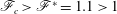 $\mathscr{F}_{c}>\mathscr{F}^{\ast }=1.1>1$
, the stretching force initially dominates and
$\mathscr{F}_{c}>\mathscr{F}^{\ast }=1.1>1$
, the stretching force initially dominates and
 $A$
decreases. However, as the thread cools, the surface tension
$A$
decreases. However, as the thread cools, the surface tension
 ${\it\gamma}({\it\theta})$
increases faster than
${\it\gamma}({\it\theta})$
increases faster than
 $\sqrt{A}$
decreases in (4.1) and eventually
$\sqrt{A}$
decreases in (4.1) and eventually
 ${\it\gamma}({\it\theta})\sqrt{A}>\mathscr{F}^{\ast }$
and thereafter
${\it\gamma}({\it\theta})\sqrt{A}>\mathscr{F}^{\ast }$
and thereafter
 $A$
increases.
$A$
increases.

Figure 2. Cooling. (a) Evolution of cross-sectional area
 $A$
with different
$A$
with different
 $\mathscr{F}^{\ast }$
, (b) evolution of temperature
$\mathscr{F}^{\ast }$
, (b) evolution of temperature
 ${\it\theta}$
with different
${\it\theta}$
with different
 $\mathscr{F}^{\ast }$
. Parameters and conditions:
$\mathscr{F}^{\ast }$
. Parameters and conditions:
 $a=0.1$
,
$a=0.1$
,
 $b=1$
,
$b=1$
,
 $H=-1$
,
$H=-1$
,
 $\mathscr{H}=1$
,
$\mathscr{H}=1$
,
 $\mathscr{F}_{c}=2.6692$
.
$\mathscr{F}_{c}=2.6692$
.
Heating. In figure 3, we also consider the case where viscosity varies more rapidly with temperature than the surface tension does (
 $b>a$
), but with heating rather than cooling. The heating causes both the surface tension and viscosity to decrease as time progresses. Using
$b>a$
), but with heating rather than cooling. The heating causes both the surface tension and viscosity to decrease as time progresses. Using
 $a=0.1$
and
$a=0.1$
and
 $b=1$
and substituting
$b=1$
and substituting
 ${\it\theta}_{h}=\infty$
into (4.9) gives
${\it\theta}_{h}=\infty$
into (4.9) gives
 $\mathscr{F}_{c}=0.8997$
. For
$\mathscr{F}_{c}=0.8997$
. For
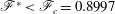 $\mathscr{F}^{\ast }<\mathscr{F}_{c}=0.8997$
,
$\mathscr{F}^{\ast }<\mathscr{F}_{c}=0.8997$
,
 $A$
will monotonically increase. Moreover, as the thread heats up, the surface tension,
$A$
will monotonically increase. Moreover, as the thread heats up, the surface tension,
 ${\it\gamma}({\it\theta})$
, decreases more slowly than
${\it\gamma}({\it\theta})$
, decreases more slowly than
 $\sqrt{A}$
increases in (4.1) and hence
$\sqrt{A}$
increases in (4.1) and hence
 ${\it\gamma}({\it\theta})\sqrt{A}-\mathscr{F}^{\ast }$
increases with time. In addition, the viscosity decreases with time and hence
${\it\gamma}({\it\theta})\sqrt{A}-\mathscr{F}^{\ast }$
increases with time. In addition, the viscosity decreases with time and hence
 $A_{{\it\tau}}$
increases with time. For
$A_{{\it\tau}}$
increases with time. For
 $\mathscr{F}^{\ast }>1$
,
$\mathscr{F}^{\ast }>1$
,
 $A$
monotonically decreases until it becomes zero in a finite time. For
$A$
monotonically decreases until it becomes zero in a finite time. For
 $1>\mathscr{F}^{\ast }>\mathscr{F}_{c}$
, the surface tension initially dominates and
$1>\mathscr{F}^{\ast }>\mathscr{F}_{c}$
, the surface tension initially dominates and
 $A$
increases. However, as the thread heats up, the surface tension
$A$
increases. However, as the thread heats up, the surface tension
 ${\it\gamma}({\it\theta})$
decreases faster than
${\it\gamma}({\it\theta})$
decreases faster than
 $\sqrt{A}$
increases in (4.1) and eventually
$\sqrt{A}$
increases in (4.1) and eventually
 ${\it\gamma}({\it\theta})\sqrt{A}<\mathscr{F}^{\ast }$
and thereafter
${\it\gamma}({\it\theta})\sqrt{A}<\mathscr{F}^{\ast }$
and thereafter
 $A$
decreases until it becomes zero in a finite time.
$A$
decreases until it becomes zero in a finite time.

Figure 3. Heating. (a) Evolution of cross-sectional area
 $A$
with different
$A$
with different
 $\mathscr{F}^{\ast }$
, (b) evolution of temperature
$\mathscr{F}^{\ast }$
, (b) evolution of temperature
 ${\it\theta}$
with different
${\it\theta}$
with different
 $\mathscr{F}^{\ast }$
. Parameters and conditions:
$\mathscr{F}^{\ast }$
. Parameters and conditions:
 $a=0.1$
,
$a=0.1$
,
 $b=1$
,
$b=1$
,
 $H=1$
,
$H=1$
,
 $\mathscr{H}=1$
,
$\mathscr{H}=1$
,
 $\mathscr{F}_{c}=0.8997$
.
$\mathscr{F}_{c}=0.8997$
.
The above study describes the dynamics of a single fluid element. All of the fluid elements evolve independently and so the dynamics appears to be simple, but the collective behaviour can still lead to a number of subtle effects. This is due to the fact that the condition for pinching depends on the evolution of viscosity and surface tension as a function of temperature. Therefore, in order to understand the dynamics of the thread, one needs to consider the dynamics of all of the fluid elements together, as described in the following subsection.
4.2 Dynamics of stretching of the fluid filament
The pinching condition for a single fluid element at location
 ${\it\xi}$
is
${\it\xi}$
is
 $\mathscr{F^{\ast}({\it\xi})}>\mathscr{F}_{c}({\it\xi})$
, or alternatively
$\mathscr{F^{\ast}({\it\xi})}>\mathscr{F}_{c}({\it\xi})$
, or alternatively
 $\mathscr{F}>\mathscr{F}_{c}({\it\xi})-\mathit{Bo}\int _{{\it\xi}}^{1}A_{0}({\it\xi}^{\prime })\,\text{d}{\it\xi}^{\prime }$
. Therefore, the critical force for the entire filament is given by
$\mathscr{F}>\mathscr{F}_{c}({\it\xi})-\mathit{Bo}\int _{{\it\xi}}^{1}A_{0}({\it\xi}^{\prime })\,\text{d}{\it\xi}^{\prime }$
. Therefore, the critical force for the entire filament is given by
 $\min _{{\it\xi}}(\mathscr{F}_{c}({\it\xi})-\mathit{Bo}\int _{{\it\xi}}^{1}A_{0}({\it\xi}^{\prime })\,\text{d}{\it\xi}^{\prime })$
. For
$\min _{{\it\xi}}(\mathscr{F}_{c}({\it\xi})-\mathit{Bo}\int _{{\it\xi}}^{1}A_{0}({\it\xi}^{\prime })\,\text{d}{\it\xi}^{\prime })$
. For
 $\mathscr{F}>\min _{{\it\xi}}(\mathscr{F}_{c}({\it\xi})-\mathit{Bo}\int _{{\it\xi}}^{1}A_{0}({\it\xi}^{\prime })\,\text{d}{\it\xi}^{\prime })$
, the thread will pinch. In order to find the time at which the thread pinches, one needs to find the fluid element that first achieves
$\mathscr{F}>\min _{{\it\xi}}(\mathscr{F}_{c}({\it\xi})-\mathit{Bo}\int _{{\it\xi}}^{1}A_{0}({\it\xi}^{\prime })\,\text{d}{\it\xi}^{\prime })$
, the thread will pinch. In order to find the time at which the thread pinches, one needs to find the fluid element that first achieves
 $A=0$
, which corresponds to finding
$A=0$
, which corresponds to finding
 $\min _{{\it\xi}}{\it\tau}_{\ast }({\it\xi})$
. The location of the pinching is then given by finding the value of
$\min _{{\it\xi}}{\it\tau}_{\ast }({\it\xi})$
. The location of the pinching is then given by finding the value of
 ${\it\xi}$
at which this is achieved, namely
${\it\xi}$
at which this is achieved, namely
 $\operatorname{argmin}_{{\it\xi}}{\it\tau}_{\ast }({\it\xi})$
.
$\operatorname{argmin}_{{\it\xi}}{\it\tau}_{\ast }({\it\xi})$
.
We now consider a set of examples that involve both heating and cooling with a viscosity that varies more rapidly with temperature than surface tension. The basic mechanisms involving thermal effects are broadly similar for both zero and non-zero
 $\mathit{Bo}$
threads. Therefore, we mostly focus on results for
$\mathit{Bo}$
threads. Therefore, we mostly focus on results for
 $\mathit{Bo}=0$
in this paper. However, we give two examples with
$\mathit{Bo}=0$
in this paper. However, we give two examples with
 $\mathit{Bo}\neq 0$
(figures 13 and 14) in the final examples at the end of § 5.
$\mathit{Bo}\neq 0$
(figures 13 and 14) in the final examples at the end of § 5.
4.2.1 Uniform heating
We first consider the case of uniform heating with two different initial conditions. In figures 4 and 5, we show results for an example with uniform heating in which the initial temperature is zero and the initial cross-section has a minimum at its midpoint. Figure 4 shows the results in Eulerian coordinates while figure 5 shows the results in Lagrangian coordinates. As one can see from figure 4, it is very hard to visualize the early time evolution clearly in Eulerian coordinates since the thread is dramatically stretched as pinching is approached. Therefore, in the rest part of the paper, we present all the results in Lagrangian coordinates except for the example (figure 12) in which spatially non-uniform heating is applied.

Figure 4. Results in Eulerian coordinates for heating with
 ${\it\theta}_{0}({\it\xi})=1$
and where
${\it\theta}_{0}({\it\xi})=1$
and where
 $A_{0}({\it\xi})$
has a minimum point. (a) Evolution of cross-sectional area
$A_{0}({\it\xi})$
has a minimum point. (a) Evolution of cross-sectional area
 $A$
, (b) evolution of temperature
$A$
, (b) evolution of temperature
 ${\it\theta}$
. Parameters and conditions used:
${\it\theta}$
. Parameters and conditions used:
 $a=0.1$
,
$a=0.1$
,
 $b=1$
,
$b=1$
,
 $H=1$
,
$H=1$
,
 $\mathscr{H}=1$
,
$\mathscr{H}=1$
,
 $A_{0}({\it\xi})=0.5+2({\it\xi}-0.5)^{2}$
,
$A_{0}({\it\xi})=0.5+2({\it\xi}-0.5)^{2}$
,
 ${\it\theta}_{0}({\it\xi})=0$
,
${\it\theta}_{0}({\it\xi})=0$
,
 $\mathscr{F}=0.645>\mathscr{F}_{c}({\it\xi}=0.5)$
,
$\mathscr{F}=0.645>\mathscr{F}_{c}({\it\xi}=0.5)$
,
 $\mathit{Bo}=0$
.
$\mathit{Bo}=0$
.

Figure 5. Results in Lagrangian coordinates for heating with
 ${\it\theta}_{0}({\it\xi})=1$
and where
${\it\theta}_{0}({\it\xi})=1$
and where
 $A_{0}({\it\xi})$
has a minimum point. (a) Evolution of cross-sectional area
$A_{0}({\it\xi})$
has a minimum point. (a) Evolution of cross-sectional area
 $A$
, (b) evolution of temperature
$A$
, (b) evolution of temperature
 ${\it\theta}$
. Parameters and conditions used:
${\it\theta}$
. Parameters and conditions used:
 $a=0.1$
,
$a=0.1$
,
 $b=1$
,
$b=1$
,
 $H=1$
,
$H=1$
,
 $\mathscr{H}=1$
,
$\mathscr{H}=1$
,
 $A_{0}({\it\xi})=0.5+2({\it\xi}-0.5)^{2}$
,
$A_{0}({\it\xi})=0.5+2({\it\xi}-0.5)^{2}$
,
 ${\it\theta}_{0}({\it\xi})=0$
,
${\it\theta}_{0}({\it\xi})=0$
,
 $\mathscr{F}=0.645>\mathscr{F}_{c}({\it\xi}=0.5)$
,
$\mathscr{F}=0.645>\mathscr{F}_{c}({\it\xi}=0.5)$
,
 $\mathit{Bo}=0$
. Note that the evolution of
$\mathit{Bo}=0$
. Note that the evolution of
 $A$
near
$A$
near
 ${\it\xi}=0.5$
is non-monotonic.
${\it\xi}=0.5$
is non-monotonic.
From figure 5, one can easily find that the cross-section of all of the fluid elements initially increases due to the small extensional force. However, the thread is thinner in the middle and the fluid elements located there heat up more rapidly than the fluid elements near the two ends. This leads to the surface tension coefficient for the fluid elements near the middle to eventually become sufficiently small that the stretching force dominates and the thread eventually pinches in the middle. The fluid elements near the ends, by contrast, cannot heat up sufficiently for the pulling force to overcome the surface tension and they therefore increase monotonically.
As our second example, we show the results in figure 6 for uniform heating in which the initial cross-section is uniform and the initial temperature has a maximum at its midpoint. In this case, the stretching force is sufficiently small that the cross-section of all fluid elements increases indefinitely. Perhaps surprisingly, the largest cross-section is neither found at the middle nor the ends of the thread. By examining (4.1), we see that this occurs as the result of two competing mechanisms. As the fluid elements heat up, the viscosity decreases more rapidly than the surface tension. On the one hand, if
 ${\it\gamma}({\it\theta})\sqrt{A}$
is sufficiently large compared with
${\it\gamma}({\it\theta})\sqrt{A}$
is sufficiently large compared with
 $\mathscr{F}$
, then the dominant effect of higher temperatures on the right-hand side of (4.1) will be to decrease the viscosity and hence the hotter elements will grow faster than the cooler elements. This explains why the fluid elements at the ends grow more slowly than their neighbours. On the other hand, if
$\mathscr{F}$
, then the dominant effect of higher temperatures on the right-hand side of (4.1) will be to decrease the viscosity and hence the hotter elements will grow faster than the cooler elements. This explains why the fluid elements at the ends grow more slowly than their neighbours. On the other hand, if
 ${\it\gamma}({\it\theta})\sqrt{A}$
is only slightly larger than
${\it\gamma}({\it\theta})\sqrt{A}$
is only slightly larger than
 $\mathscr{F}$
, then the dominant effect of higher temperatures will be to reduce the numerator in the right-hand side of (4.1) and hence the hotter elements will grow more slowly than the cooler elements. This explains why the fluid elements in the middle grow more slowly than their neighbours. These two effects combine to generate the two local maxima observed in figure 6.
$\mathscr{F}$
, then the dominant effect of higher temperatures will be to reduce the numerator in the right-hand side of (4.1) and hence the hotter elements will grow more slowly than the cooler elements. This explains why the fluid elements in the middle grow more slowly than their neighbours. These two effects combine to generate the two local maxima observed in figure 6.

Figure 6. Results for heating when
 ${\it\theta}_{0}({\it\xi})$
has a local maximum and
${\it\theta}_{0}({\it\xi})$
has a local maximum and
 $A_{0}({\it\xi})=1$
. (a) Evolution of cross-sectional area
$A_{0}({\it\xi})=1$
. (a) Evolution of cross-sectional area
 $A$
, (b) evolution of temperature
$A$
, (b) evolution of temperature
 ${\it\theta}$
. Parameters and conditions used:
${\it\theta}$
. Parameters and conditions used:
 $a=0.1$
,
$a=0.1$
,
 $b=1$
,
$b=1$
,
 $H=1$
,
$H=1$
,
 $\mathscr{H}=1$
,
$\mathscr{H}=1$
,
 $A_{0}({\it\xi})=1$
,
$A_{0}({\it\xi})=1$
,
 ${\it\theta}_{0}({\it\xi})=\exp (-({\it\xi}-0.5)^{2})$
,
${\it\theta}_{0}({\it\xi})=\exp (-({\it\xi}-0.5)^{2})$
,
 $\mathscr{F}=0.84<\mathscr{F}_{c}({\it\xi}=0.5)$
,
$\mathscr{F}=0.84<\mathscr{F}_{c}({\it\xi}=0.5)$
,
 $\mathit{Bo}=0$
.
$\mathit{Bo}=0$
.
4.2.2 Uniform cooling
In figure 7, we show results for an example with uniform cooling in which the initial cross-section is uniform and the initial temperature has a maximum at its midpoint. In this case, the stretching force is sufficiently large that all fluid elements will monotonically thin with time. The hottest fluid elements that are initially near the middle have smaller surface tension than the fluid elements near the ends. This means that they are more strongly affected by the stretching force and hence thin more rapidly. Since these elements have thinner cross-section, they are more rapidly affected by the external cooling than the fluid elements that were initially cooler. When pinching occurs, the fluid elements in the middle become the coolest in the entire thread as observed in figure 7.

Figure 7. Results for cooling when
 ${\it\theta}_{0}({\it\xi})$
has a local maximum and
${\it\theta}_{0}({\it\xi})$
has a local maximum and
 $A_{0}({\it\xi})=1$
. (a) Evolution of cross-sectional area
$A_{0}({\it\xi})=1$
. (a) Evolution of cross-sectional area
 $A$
, (b) evolution of temperature
$A$
, (b) evolution of temperature
 ${\it\theta}$
. Parameters and conditions used:
${\it\theta}$
. Parameters and conditions used:
 $a=0.1$
,
$a=0.1$
,
 $b=1$
,
$b=1$
,
 $H=-1$
,
$H=-1$
,
 $\mathscr{H}=1$
,
$\mathscr{H}=1$
,
 $A_{0}({\it\xi})=1$
,
$A_{0}({\it\xi})=1$
,
 ${\it\theta}_{0}({\it\xi})=-({\it\xi}-0.5)^{2}$
,
${\it\theta}_{0}({\it\xi})=-({\it\xi}-0.5)^{2}$
,
 $\mathscr{F}=3>\mathscr{F}_{c}({\it\xi}=0.5)$
,
$\mathscr{F}=3>\mathscr{F}_{c}({\it\xi}=0.5)$
,
 $\mathit{Bo}=0$
.
$\mathit{Bo}=0$
.
5 Inertial effects
When
 $\mathit{Re}=0$
and
$\mathit{Re}=0$
and
 $H=H({\it\theta})$
, all the fluid elements evolve independently and satisfy (4.1) and (4.3). However, when
$H=H({\it\theta})$
, all the fluid elements evolve independently and satisfy (4.1) and (4.3). However, when
 $Re\neq 0$
, this is no longer true. The effects of inertia can be most readily understood by considering the integral of (3.7) with respect to
$Re\neq 0$
, this is no longer true. The effects of inertia can be most readily understood by considering the integral of (3.7) with respect to
 ${\it\xi}$
. After applying the boundary condition of fixed extensional force at the free end point
${\it\xi}$
. After applying the boundary condition of fixed extensional force at the free end point
 ${\it\xi}=1$
, we obtain
${\it\xi}=1$
, we obtain
 $$\begin{eqnarray}\mathscr{F}+\mathit{Bo}\int _{{\it\xi}}^{1}A_{0}({\it\xi}^{\prime })\,\text{d}{\it\xi}^{\prime }-\mathit{Re}\frac{\partial }{\partial {\it\tau}}\left[\int _{{\it\xi}}^{1}A_{0}({\it\xi}^{\prime })u({\it\xi}^{\prime },{\it\tau})\,\text{d}{\it\xi}^{\prime }\right]=-{\it\mu}({\it\theta})A_{{\it\tau}}+{\it\gamma}({\it\theta})\sqrt{A}.\end{eqnarray}$$
If
 $\mathit{Re}=0$
, the effective stretching force on the left-hand side of (5.1) is the function
$\mathit{Re}=0$
, the effective stretching force on the left-hand side of (5.1) is the function
 $\mathscr{F}^{\ast }({\it\xi})$
. This corresponds to the stretching force imposed at the free end point being perfectly transmitted throughout the length of the thread. If
$\mathscr{F}^{\ast }({\it\xi})$
. This corresponds to the stretching force imposed at the free end point being perfectly transmitted throughout the length of the thread. If
 $\mathit{Re}\neq 0$
, then the effective stretching force will be modified by the integral on the left-hand side of (5.1). For
$\mathit{Re}\neq 0$
, then the effective stretching force will be modified by the integral on the left-hand side of (5.1). For
 $\mathit{Re}\ll 1$
, this effective force modification will be small and the motion will be well approximated by the
$\mathit{Re}\ll 1$
, this effective force modification will be small and the motion will be well approximated by the
 $\mathit{Re}=0$
solution unless the extension of the thread becomes sufficiently large that the acceleration
$\mathit{Re}=0$
solution unless the extension of the thread becomes sufficiently large that the acceleration
 $\partial u/\partial {\it\tau}$
becomes of
$\partial u/\partial {\it\tau}$
becomes of
 $O(\mathit{Re}^{-1})$
, which corresponds to
$O(\mathit{Re}^{-1})$
, which corresponds to
 $A$
becoming small. When this occurs, the stretching force will not be transmitted effectively through the regions of small
$A$
becoming small. When this occurs, the stretching force will not be transmitted effectively through the regions of small
 $A$
and the stretching will be reduced.
$A$
and the stretching will be reduced.
We now show the results of numerical simulations that illustrate the phenomena that can occur when inertia is included. In order to solve (3.6)–(3.9) numerically, we spatially discretized (3.6)–(3.8) using second-order central differences. We then solved the resulting system of ordinary differential equations with a standard numerical solver. At each time step, we integrated (3.9) using a trapezoid rule to obtain the relation between the Lagrangian and Eulerian coordinates. We note that if the heater is spatially uniform, then (3.9) decouples from (3.6)–(3.8). The grid points are uniformly distributed in the Lagrangian coordinate and so if the thread becomes highly extended in some regions, then the distance between neighbouring grid points in Eulerian space will become large. This phenomena has been shown to lead to numerical inaccuracies (Stokes & Tuck Reference Stokes and Tuck2004) when dealing with the Lagrangian equations. In order to prevent this, if the grid spacing exceeded a threshold, we used linear interpolation to add additional grid points in the affected regions.
5.1 Thinning under spatially uniform conditions
We begin by considering the case in which
 $A_{0}({\it\xi})=1$
and
$A_{0}({\it\xi})=1$
and
 ${\it\theta}_{0}({\it\xi})=0$
with a spatially uniform heater and an extensional force larger than the critical value. If inertia is completely neglected, then all fluid elements will behave in an identical way and the thread will thin in a spatially uniform way. For
${\it\theta}_{0}({\it\xi})=0$
with a spatially uniform heater and an extensional force larger than the critical value. If inertia is completely neglected, then all fluid elements will behave in an identical way and the thread will thin in a spatially uniform way. For
 $\mathit{Re}=0.001$
used in figure 8, the early evolution is well approximated by spatially uniform thinning. However, when the thread thins sufficiently, inertial effects reduce the effective stretching force as one moves away from the pulled end. This implies that the rate of thinning will be largest at the pulled end and so
$\mathit{Re}=0.001$
used in figure 8, the early evolution is well approximated by spatially uniform thinning. However, when the thread thins sufficiently, inertial effects reduce the effective stretching force as one moves away from the pulled end. This implies that the rate of thinning will be largest at the pulled end and so
 $A$
will first become zero at the free end of the thread. This is seen to occur in the later stages of stretching in figure 8.
$A$
will first become zero at the free end of the thread. This is seen to occur in the later stages of stretching in figure 8.

Figure 8. Numerical results for a thread with initially uniform radius and temperature subjected to spatially uniform heating. (a) Evolution of
 $A$
. (b) Evolution of
$A$
. (b) Evolution of
 ${\it\theta}$
. Parameters and conditions used:
${\it\theta}$
. Parameters and conditions used:
 $a=0.1$
,
$a=0.1$
,
 $b=1$
,
$b=1$
,
 $A_{0}({\it\xi})=1$
,
$A_{0}({\it\xi})=1$
,
 ${\it\theta}_{0}({\it\xi})=0$
,
${\it\theta}_{0}({\it\xi})=0$
,
 $\mathscr{F}=1.0005$
,
$\mathscr{F}=1.0005$
,
 $\mathit{Re}=0.001$
,
$\mathit{Re}=0.001$
,
 $H=2-{\it\theta}$
,
$H=2-{\it\theta}$
,
 $\mathscr{H}=1$
,
$\mathscr{H}=1$
,
 $\mathit{Bo}=0$
.
$\mathit{Bo}=0$
.

Figure 9. Numerical results for a uniform thread whose initial temperature
 ${\it\theta}_{0}({\it\xi})$
is maximum at the upper boundary point
${\it\theta}_{0}({\it\xi})$
is maximum at the upper boundary point
 ${\it\xi}=0$
. (a,b)
${\it\xi}=0$
. (a,b)
 $\mathit{Re}=0.01$
(small
$\mathit{Re}=0.01$
(small
 $\mathit{Re}$
), pinching happens at the hottest point, i.e.
$\mathit{Re}$
), pinching happens at the hottest point, i.e.
 ${\it\xi}=0$
. (c,d)
${\it\xi}=0$
. (c,d)
 $\mathit{Re}=10$
(relatively large
$\mathit{Re}=10$
(relatively large
 $\mathit{Re}$
), pinching happens at the pulled end. Parameters and conditions used:
$\mathit{Re}$
), pinching happens at the pulled end. Parameters and conditions used:
 $a=0.1$
,
$a=0.1$
,
 $b=1$
,
$b=1$
,
 $A_{0}({\it\xi})=1$
,
$A_{0}({\it\xi})=1$
,
 ${\it\theta}_{0}({\it\xi})=2(1-{\it\xi}^{2})$
,
${\it\theta}_{0}({\it\xi})=2(1-{\it\xi}^{2})$
,
 $\mathscr{F}=1.1$
,
$\mathscr{F}=1.1$
,
 $H({\it\theta})=-{\it\theta}$
,
$H({\it\theta})=-{\it\theta}$
,
 $\mathscr{H}=1$
,
$\mathscr{H}=1$
,
 $\mathit{Bo}=0$
.
$\mathit{Bo}=0$
.

Figure 10. Numerical results for a thread whose initial temperature
 ${\it\theta}_{0}({\it\xi})$
is two different constants near the two end points and has a rapid transition near
${\it\theta}_{0}({\it\xi})$
is two different constants near the two end points and has a rapid transition near
 ${\it\xi}=0.5$
. (a,b)
${\it\xi}=0.5$
. (a,b)
 $\mathit{Re}=1$
(relatively small
$\mathit{Re}=1$
(relatively small
 $\mathit{Re}$
), pinching happens at the fluid element that initially had a large temperature gradient, i.e.
$\mathit{Re}$
), pinching happens at the fluid element that initially had a large temperature gradient, i.e.
 ${\it\xi}=0.5$
. (c,d)
${\it\xi}=0.5$
. (c,d)
 $\mathit{Re}=20$
(relatively large
$\mathit{Re}=20$
(relatively large
 $\mathit{Re}$
), pinching happens at the pulled end. Parameters and conditions used:
$\mathit{Re}$
), pinching happens at the pulled end. Parameters and conditions used:
 $a=0.1$
,
$a=0.1$
,
 $b=1$
,
$b=1$
,
 $A_{0}({\it\xi})=1$
,
$A_{0}({\it\xi})=1$
,
 ${\it\theta}_{0}({\it\xi})=2(1+\tanh ((0.5-{\it\xi})/{\it\epsilon}))$
,
${\it\theta}_{0}({\it\xi})=2(1+\tanh ((0.5-{\it\xi})/{\it\epsilon}))$
,
 ${\it\epsilon}=0.04$
,
${\it\epsilon}=0.04$
,
 $\mathscr{F}=1.1$
,
$\mathscr{F}=1.1$
,
 $H({\it\theta})=-{\it\theta}$
,
$H({\it\theta})=-{\it\theta}$
,
 $\mathscr{H}=1$
,
$\mathscr{H}=1$
,
 $\mathit{Bo}=0$
.
$\mathit{Bo}=0$
.
5.2 Thinning under non-uniform initial temperature
In this subsection, we will use a set of examples to illustrate that the pinching location for a preheated thread with non-zero Reynolds number is determined by three different mechanisms: extensional force-driven pinching, surface-tension-driven pinching and largest-temperature-gradient-driven pinching.
Extensional force-driven pinching versus surface-tension-driven pinching. We consider a case with an initially uniform cross-section,
 $A_{0}({\it\xi})=1$
, a spatially uniform heater, a stretching force greater than the critical value and an initial temperature profile with the maximum at the upper boundary of the thread. For a small
$A_{0}({\it\xi})=1$
, a spatially uniform heater, a stretching force greater than the critical value and an initial temperature profile with the maximum at the upper boundary of the thread. For a small
 $\mathit{Re}=0.01$
(figure 9
a), the motion is very similar to the
$\mathit{Re}=0.01$
(figure 9
a), the motion is very similar to the
 $\mathit{Re}=0$
behaviour until the thread becomes thin, the thread then undergoes surface-tension-driven pinching at the upper boundary of the thread. However, for a larger
$\mathit{Re}=0$
behaviour until the thread becomes thin, the thread then undergoes surface-tension-driven pinching at the upper boundary of the thread. However, for a larger
 $\mathit{Re}=10$
, the situation is different (figure 9
c). The inertial effects are significant even in the early stages of pulling and this means that the stretching force is far from being uniformly transmitted through the length of the thread. This implies that stretching is much more significant near the pulled end of the thread and this causes the cross-sectional area to become zero at the pulled end. Hence, for small
$\mathit{Re}=10$
, the situation is different (figure 9
c). The inertial effects are significant even in the early stages of pulling and this means that the stretching force is far from being uniformly transmitted through the length of the thread. This implies that stretching is much more significant near the pulled end of the thread and this causes the cross-sectional area to become zero at the pulled end. Hence, for small
 $\mathit{Re}$
the thread will pinch at the hottest point, whereas for larger
$\mathit{Re}$
the thread will pinch at the hottest point, whereas for larger
 $\mathit{Re}$
the thread will pinch at the pulled end.
$\mathit{Re}$
the thread will pinch at the pulled end.
Extensional force-driven pinching versus largest-temperature-gradient-driven pinching. In this case, we will show that another mechanism can also affect the place where the pinching occurs. Again, we consider an initially uniform cross-section,
 $A_{0}({\it\xi})=1$
, a spatially uniform heater and a stretching force greater than the critical value. However, in this case, we adopt an initial temperature profile that is uniformly hot near the upper boundary of the thread and uniformly cool near the pulled end. The two constant regions are joined together by a thin transition region. For a relatively large
$A_{0}({\it\xi})=1$
, a spatially uniform heater and a stretching force greater than the critical value. However, in this case, we adopt an initial temperature profile that is uniformly hot near the upper boundary of the thread and uniformly cool near the pulled end. The two constant regions are joined together by a thin transition region. For a relatively large
 $\mathit{Re}=20$
(figure 10
c), the behaviour is similar to that shown in the previous example, with significant thinning near the pulled end of the thread until the cross-sectional area becomes zero there. However, for a relatively small
$\mathit{Re}=20$
(figure 10
c), the behaviour is similar to that shown in the previous example, with significant thinning near the pulled end of the thread until the cross-sectional area becomes zero there. However, for a relatively small
 $\mathit{Re}=1$
(figure 10
a), the behaviour is quite different. Using (3.6), we can rewrite (3.7) for
$\mathit{Re}=1$
(figure 10
a), the behaviour is quite different. Using (3.6), we can rewrite (3.7) for
 $\mathit{Bo}=0$
in the form
$\mathit{Bo}=0$
in the form
 $$\begin{eqnarray}Reu_{{\it\tau}}=\frac{1}{A_{0}}\left({\it\mu}({\it\theta})\frac{A^{2}}{A_{0}}u_{{\it\xi}}+{\it\gamma}({\it\theta})\sqrt{A}\right)_{{\it\xi}}.\end{eqnarray}$$
Since we chose initial conditions
 $u({\it\xi},0)=0$
and
$u({\it\xi},0)=0$
and
 $A({\it\xi},0)=1$
, we see that during the very early stages of the dynamics, the right-hand side of (5.2) is dominated by the surface tension force term
$A({\it\xi},0)=1$
, we see that during the very early stages of the dynamics, the right-hand side of (5.2) is dominated by the surface tension force term
 $({\it\gamma}({\it\theta})\sqrt{A})_{{\it\xi}}$
. For the temperature profile we have chosen, the surface tension will be small and constant near the upper boundary of the thread, large and constant near the pulled end of the thread and have a large slope in the thin transition region. This gradient in the surface tension will initially cause an acceleration of the fluid elements in the transition region towards the pulled end of the thread. Since mass must be conserved, this acceleration causes thinning of the fluid elements on the hot side of the transition region and broadening of the fluid elements on the cool side of the region. Therefore, during the initial stages, there is a local minimum in the cross-section on the hot side of the transition region and a local maximum on the cool side. The thread then is stretched by the imposed force until a fluid element on the hot side of the transition region experiences pinching. We note that if the initial temperature profile had been such that the thread was cooler near the upper boundary and hotter near the pulled end, then the surface tension would have been initially large near the upper boundary and small near the pulled end. This would induce accelerations in the transition regions away from the pulled end. Therefore, we would also observe pinching in the fluid elements on the hot side of the transition region.
$({\it\gamma}({\it\theta})\sqrt{A})_{{\it\xi}}$
. For the temperature profile we have chosen, the surface tension will be small and constant near the upper boundary of the thread, large and constant near the pulled end of the thread and have a large slope in the thin transition region. This gradient in the surface tension will initially cause an acceleration of the fluid elements in the transition region towards the pulled end of the thread. Since mass must be conserved, this acceleration causes thinning of the fluid elements on the hot side of the transition region and broadening of the fluid elements on the cool side of the region. Therefore, during the initial stages, there is a local minimum in the cross-section on the hot side of the transition region and a local maximum on the cool side. The thread then is stretched by the imposed force until a fluid element on the hot side of the transition region experiences pinching. We note that if the initial temperature profile had been such that the thread was cooler near the upper boundary and hotter near the pulled end, then the surface tension would have been initially large near the upper boundary and small near the pulled end. This would induce accelerations in the transition regions away from the pulled end. Therefore, we would also observe pinching in the fluid elements on the hot side of the transition region.
Extensional force-driven pinching versus largest-temperature-gradient-driven pinching versus surface-tension-driven pinching. On the one hand, figure 9 illustrated how pinching can occur in the hottest region for a small
 $\mathit{Re}$
and at the pulled end for a larger
$\mathit{Re}$
and at the pulled end for a larger
 $\mathit{Re}$
. On the other hand, figure 10 illustrated how pinching can occur near the large temperature gradients for a relatively small
$\mathit{Re}$
. On the other hand, figure 10 illustrated how pinching can occur near the large temperature gradients for a relatively small
 $\mathit{Re}$
and at the pulled end for a relatively large
$\mathit{Re}$
and at the pulled end for a relatively large
 $\mathit{Re}$
. Therefore, there are three possible mechanisms: at a relatively large
$\mathit{Re}$
. Therefore, there are three possible mechanisms: at a relatively large
 $\mathit{Re}$
, the force transmission is weak and the thread will tend to pinch at the pulled end; for a relatively small
$\mathit{Re}$
, the force transmission is weak and the thread will tend to pinch at the pulled end; for a relatively small
 $\mathit{Re}$
the hottest part of the thread will have the lowest viscosity and weakest surface tension and so will tend to pinch there; and for an intermediate
$\mathit{Re}$
the hottest part of the thread will have the lowest viscosity and weakest surface tension and so will tend to pinch there; and for an intermediate
 $\mathit{Re}$
, if there are large gradients in temperature, accelerations can be induced that lead to pinching in fluid elements near the large gradients.
$\mathit{Re}$
, if there are large gradients in temperature, accelerations can be induced that lead to pinching in fluid elements near the large gradients.
We now consider an example that includes a competition between all three of the mechanisms illustrated in the previous two examples. To do this, we take an initial temperature profile with a maximum at the upper boundary of the thread but with a sharp transition to lower temperatures (see the initial temperature function
 ${\it\theta}_{0}({\it\xi})$
in figure 11
b). For a small
${\it\theta}_{0}({\it\xi})$
in figure 11
b). For a small
 $\mathit{Re}=0.01$
, the acceleration induced near the sharp transition is sufficiently small that the minimum cross-section is always located at the upper boundary (at the hottest point) and the thread ultimately pinches there (figure 11
a). We note that at early times, the cross-sectional area of all of the fluid elements decreases with time. In fact, during early times,
$\mathit{Re}=0.01$
, the acceleration induced near the sharp transition is sufficiently small that the minimum cross-section is always located at the upper boundary (at the hottest point) and the thread ultimately pinches there (figure 11
a). We note that at early times, the cross-sectional area of all of the fluid elements decreases with time. In fact, during early times,
 $A$
is well approximated by the inertialess evolution equation (4.1) and there are no significant accelerations induced by the temperature gradients. This is because
$A$
is well approximated by the inertialess evolution equation (4.1) and there are no significant accelerations induced by the temperature gradients. This is because
 $\mathit{Re}$
is small and
$\mathit{Re}$
is small and
 $A=O(1)$
. However, at later times, when
$A=O(1)$
. However, at later times, when
 $A$
becomes smaller, accelerations do become significant and cause the thread to thin on the hot side of the transition and thicken on the cool side of the transition, but the effect is too weak to cause pinching to occur on the hot side of the transition. For an intermediate
$A$
becomes smaller, accelerations do become significant and cause the thread to thin on the hot side of the transition and thicken on the cool side of the transition, but the effect is too weak to cause pinching to occur on the hot side of the transition. For an intermediate
 $\mathit{Re}=1$
, the acceleration induced by the surface tension gradient is large enough that the minimum cross-section occurs near the transition and the thread therefore pinches near the transition region (figure 11
c). Finally, for a relatively large
$\mathit{Re}=1$
, the acceleration induced by the surface tension gradient is large enough that the minimum cross-section occurs near the transition and the thread therefore pinches near the transition region (figure 11
c). Finally, for a relatively large
 $\mathit{Re}=20$
, the transmission of the stretching force is sufficiently weak that the thread pinches at the pulled end (figure 11
e). We have therefore shown that the location at which pinching occurs is quite subtly affected by
$\mathit{Re}=20$
, the transmission of the stretching force is sufficiently weak that the thread pinches at the pulled end (figure 11
e). We have therefore shown that the location at which pinching occurs is quite subtly affected by
 $\mathit{Re}$
.
$\mathit{Re}$
.

Figure 11. Numerical results for a thread whose initial temperature
 ${\it\theta}_{0}({\it\xi})$
is maximum at the upper boundary point
${\it\theta}_{0}({\it\xi})$
is maximum at the upper boundary point
 ${\it\xi}=0$
and has a rapid transition down to zero near
${\it\xi}=0$
and has a rapid transition down to zero near
 ${\it\xi}=0.5$
. (a,b)
${\it\xi}=0.5$
. (a,b)
 $\mathit{Re}=0.01$
(small
$\mathit{Re}=0.01$
(small
 $\mathit{Re}$
), pinching happens at the hottest point, i.e.
$\mathit{Re}$
), pinching happens at the hottest point, i.e.
 ${\it\xi}=0$
. (c,d)
${\it\xi}=0$
. (c,d)
 $\mathit{Re}=1$
(intermediate
$\mathit{Re}=1$
(intermediate
 $\mathit{Re}$
), pinching happens for a fluid element that was initially near the large temperature gradient, i.e.
$\mathit{Re}$
), pinching happens for a fluid element that was initially near the large temperature gradient, i.e.
 ${\it\xi}=0.5$
. (e,f)
${\it\xi}=0.5$
. (e,f)
 $\mathit{Re}=20$
(relatively large
$\mathit{Re}=20$
(relatively large
 $\mathit{Re}$
), pinching happens at the pulled end. Parameters and conditions used:
$\mathit{Re}$
), pinching happens at the pulled end. Parameters and conditions used:
 $a=0.1$
,
$a=0.1$
,
 $b=1$
,
$b=1$
,
 $A_{0}({\it\xi})=1$
,
$A_{0}({\it\xi})=1$
,
 ${\it\theta}_{0}({\it\xi})=8/3(1-{\it\xi}^{2})(1+\tanh ((0.5-{\it\xi})/{\it\epsilon}))/2$
,
${\it\theta}_{0}({\it\xi})=8/3(1-{\it\xi}^{2})(1+\tanh ((0.5-{\it\xi})/{\it\epsilon}))/2$
,
 ${\it\epsilon}=0.01$
,
${\it\epsilon}=0.01$
,
 $\mathscr{F}=1.1$
,
$\mathscr{F}=1.1$
,
 $H({\it\theta})=-{\it\theta}$
,
$H({\it\theta})=-{\it\theta}$
,
 $\mathscr{H}=1$
,
$\mathscr{H}=1$
,
 $\mathit{Bo}=0$
.
$\mathit{Bo}=0$
.

Figure 12. Numerical results for a thread with initially uniform radius and uniform temperature but with spatially non-uniform heating, where the external heater temperature
 ${\it\theta}_{h}$
is maximum at the upper boundary
${\it\theta}_{h}$
is maximum at the upper boundary
 $x=0$
and has a rapid transition to zero near
$x=0$
and has a rapid transition to zero near
 $x=0.5$
. (a,b)
$x=0.5$
. (a,b)
 $\mathit{Re}=0.01$
(small
$\mathit{Re}=0.01$
(small
 $\mathit{Re}$
), pinching happens at the hottest point, i.e.
$\mathit{Re}$
), pinching happens at the hottest point, i.e.
 $x=0$
. (c,d)
$x=0$
. (c,d)
 $\mathit{Re}=10$
(moderately large
$\mathit{Re}=10$
(moderately large
 $\mathit{Re}$
), pinching happens for a fluid element that was initially near the large temperature gradient
$\mathit{Re}$
), pinching happens for a fluid element that was initially near the large temperature gradient
 $x=0.5$
. (e,f)
$x=0.5$
. (e,f)
 $\mathit{Re}=100$
(large
$\mathit{Re}=100$
(large
 $\mathit{Re}$
), pinching happens at the pulled end. Parameters and conditions used:
$\mathit{Re}$
), pinching happens at the pulled end. Parameters and conditions used:
 $a=0.1$
,
$a=0.1$
,
 $b=1$
,
$b=1$
,
 $A_{0}({\it\xi})=1$
,
$A_{0}({\it\xi})=1$
,
 ${\it\theta}_{0}({\it\xi})=0$
,
${\it\theta}_{0}({\it\xi})=0$
,
 $\mathscr{F}=1.05$
,
$\mathscr{F}=1.05$
,
 $H({\it\theta})=1.05(1-3x^{2})(1+\tanh ((0.5-x)/{\it\epsilon}))-{\it\theta}$
,
$H({\it\theta})=1.05(1-3x^{2})(1+\tanh ((0.5-x)/{\it\epsilon}))-{\it\theta}$
,
 ${\it\epsilon}=0.04$
,
${\it\epsilon}=0.04$
,
 $\mathscr{H}=1$
,
$\mathscr{H}=1$
,
 $\mathit{Bo}=0$
.
$\mathit{Bo}=0$
.
5.3 Thinning under non-uniform heating
In this subsection, we present results for the case of a non-uniform heater in figure 12. We will use an example to illustrate that the competition seen in the above examples can also occur in this case. We consider initial conditions that are spatially uniform,
 $A_{0}({\it\xi})=1$
and
$A_{0}({\it\xi})=1$
and
 ${\it\theta}_{0}({\it\xi})=0$
with an extensional force larger than the critical value. We choose a heater profile that has a high heating rate in a finite region near the upper boundary of the thread with a local maximum at the upper boundary and a rapid transition to a lower heating rate outside of the finite region, see figure 12. In some ways, the dynamics is very similar to the preheated case, but there is an important difference. Fluid elements that start in the region with large heating rate heat up and experience lower surface tension and have lower viscosities and hence thin more rapidly than fluid elements that start in the region with lower heating rate. However, this thinning causes the fluid elements to extend and hence move out of the region with large heating rate. Only the fluid elements very close to the centreline experience strong heating for extended lengths of times. This results in a smoothing effect on the temperature profiles in the thread and tends to reduce the magnitude of the mechanism associated with temperature gradients that caused pinching in the preheated case. If the heating rate does not have an especially large spatial gradient, then small
${\it\theta}_{0}({\it\xi})=0$
with an extensional force larger than the critical value. We choose a heater profile that has a high heating rate in a finite region near the upper boundary of the thread with a local maximum at the upper boundary and a rapid transition to a lower heating rate outside of the finite region, see figure 12. In some ways, the dynamics is very similar to the preheated case, but there is an important difference. Fluid elements that start in the region with large heating rate heat up and experience lower surface tension and have lower viscosities and hence thin more rapidly than fluid elements that start in the region with lower heating rate. However, this thinning causes the fluid elements to extend and hence move out of the region with large heating rate. Only the fluid elements very close to the centreline experience strong heating for extended lengths of times. This results in a smoothing effect on the temperature profiles in the thread and tends to reduce the magnitude of the mechanism associated with temperature gradients that caused pinching in the preheated case. If the heating rate does not have an especially large spatial gradient, then small
 $\mathit{Re}$
solutions will pinch at the upper boundary and large
$\mathit{Re}$
solutions will pinch at the upper boundary and large
 $\mathit{Re}$
solutions will pinch at the pulled end point. Nevertheless, if we choose the transition zone in the heating rate to be sufficiently narrow, the surface-tension-gradient effect will cause pinching to occur to fluid elements that started near the edge of the transition zone, see figure 12.
$\mathit{Re}$
solutions will pinch at the pulled end point. Nevertheless, if we choose the transition zone in the heating rate to be sufficiently narrow, the surface-tension-gradient effect will cause pinching to occur to fluid elements that started near the edge of the transition zone, see figure 12.

Figure 13. Numerical results for a thread falling under gravity with non-zero stretching force and initially uniform temperature. (a,b)
 $\mathit{Re}=0.1$
(small
$\mathit{Re}=0.1$
(small
 $\mathit{Re}$
), pinching occurs at the top, i.e.
$\mathit{Re}$
), pinching occurs at the top, i.e.
 ${\it\xi}=0$
. (c,d)
${\it\xi}=0$
. (c,d)
 $\mathit{Re}=10$
(relatively large
$\mathit{Re}=10$
(relatively large
 $\mathit{Re}$
), pinching occurs at the pulled end, i.e.
$\mathit{Re}$
), pinching occurs at the pulled end, i.e.
 ${\it\xi}=1$
. Parameters and conditions used:
${\it\xi}=1$
. Parameters and conditions used:
 $a=0.1$
,
$a=0.1$
,
 $b=1$
,
$b=1$
,
 $A_{0}({\it\xi})=1$
,
$A_{0}({\it\xi})=1$
,
 ${\it\theta}_{0}({\it\xi})=0$
,
${\it\theta}_{0}({\it\xi})=0$
,
 $\mathscr{F}=1.1$
,
$\mathscr{F}=1.1$
,
 $H({\it\theta})=3-{\it\theta}$
,
$H({\it\theta})=3-{\it\theta}$
,
 $\mathscr{H}=1$
,
$\mathscr{H}=1$
,
 $\mathit{Bo}=1$
.
$\mathit{Bo}=1$
.

Figure 14. Numerical results for a thread falling under gravity with zero stretching force and non-uniform initial temperature, where the initial temperature
 ${\it\theta}_{0}({\it\xi})$
has a rapid transition near
${\it\theta}_{0}({\it\xi})$
has a rapid transition near
 ${\it\xi}=0.5$
. (a,b)
${\it\xi}=0.5$
. (a,b)
 $\mathit{Re}=1$
(small
$\mathit{Re}=1$
(small
 $\mathit{Re}$
), pinching happens at the top end due to the weight of the thread. (c,d)
$\mathit{Re}$
), pinching happens at the top end due to the weight of the thread. (c,d)
 $\mathit{Re}=100$
(large
$\mathit{Re}=100$
(large
 $\mathit{Re}$
), pinching occurs at a fluid element that was initially near the large temperature gradient. Parameters and conditions used:
$\mathit{Re}$
), pinching occurs at a fluid element that was initially near the large temperature gradient. Parameters and conditions used:
 $a=0.1$
,
$a=0.1$
,
 $b=1$
,
$b=1$
,
 $A_{0}({\it\xi})=1$
,
$A_{0}({\it\xi})=1$
,
 ${\it\theta}_{0}({\it\xi})=3(1+\tanh ((0.5-{\it\xi})/{\it\epsilon}))/2$
,
${\it\theta}_{0}({\it\xi})=3(1+\tanh ((0.5-{\it\xi})/{\it\epsilon}))/2$
,
 ${\it\epsilon}=0.005$
,
${\it\epsilon}=0.005$
,
 $\mathscr{F}=0$
,
$\mathscr{F}=0$
,
 $H({\it\theta})=-{\it\theta}$
,
$H({\it\theta})=-{\it\theta}$
,
 $\mathscr{H}=1$
,
$\mathscr{H}=1$
,
 $\mathit{Bo}=0.5$
.
$\mathit{Bo}=0.5$
.
5.4 Thinning with non-zero gravity
Finally, in this subsection, we consider two examples with non-zero
 $\mathit{Bo}$
as shown in figures 13 and 14. Figure 13 shows the case in which the thread is falling under gravity with a non-zero stretching force. The thread has initially uniform temperature and radius and is subjected to spatially uniform external heating from the environment. The stretching force applied at the pulled end is chosen to be greater than the critical value so that pinching would occur at the free end in the absence of gravity. The results are qualitatively similar to the
$\mathit{Bo}$
as shown in figures 13 and 14. Figure 13 shows the case in which the thread is falling under gravity with a non-zero stretching force. The thread has initially uniform temperature and radius and is subjected to spatially uniform external heating from the environment. The stretching force applied at the pulled end is chosen to be greater than the critical value so that pinching would occur at the free end in the absence of gravity. The results are qualitatively similar to the
 $\mathit{Bo}=0$
case in the sense that, depending on
$\mathit{Bo}=0$
case in the sense that, depending on
 $\mathit{Re}$
, pinching can happen either at the top or at the pulled end. For
$\mathit{Re}$
, pinching can happen either at the top or at the pulled end. For
 $\mathit{Re}=0$
, the dynamics of the cross-sectional area is determined by (4.1) and (4.2) and the maximum extensional force occurs at the top of the thread where the supported weight is maximal. This means that an initially uniform thread with uniform heating will always pinch at the top. For sufficiently small
$\mathit{Re}=0$
, the dynamics of the cross-sectional area is determined by (4.1) and (4.2) and the maximum extensional force occurs at the top of the thread where the supported weight is maximal. This means that an initially uniform thread with uniform heating will always pinch at the top. For sufficiently small
 $\mathit{Re}$
, inertia plays a small role and pinching is observed to occur at the top (figure 13
a). For larger
$\mathit{Re}$
, inertia plays a small role and pinching is observed to occur at the top (figure 13
a). For larger
 $\mathit{Re}$
, the force applied at the end of the thread is not uniformly transmitted through the thread. Inertia also acts to reduce the effective stretching force due to gravity. This means that the stretching force at the top will be reduced by inertia. At the free end of the thread, the force is fixed and so inertia has no effect. Therefore, for sufficiently large
$\mathit{Re}$
, the force applied at the end of the thread is not uniformly transmitted through the thread. Inertia also acts to reduce the effective stretching force due to gravity. This means that the stretching force at the top will be reduced by inertia. At the free end of the thread, the force is fixed and so inertia has no effect. Therefore, for sufficiently large
 $\mathit{Re}$
, we expect that pinching will happen at the pulled end. This is observed for
$\mathit{Re}$
, we expect that pinching will happen at the pulled end. This is observed for
 $\mathit{Re}=10$
in figure 13(c).
$\mathit{Re}=10$
in figure 13(c).
In figure 14, we consider a case with initially uniform radius and uniform environment, but an initial temperature profile with a sharp transition. However, rather than using a non-zero extensional force at the pulled end with zero gravity (as we used in figures 8–11), we use zero extensional force
 $\mathscr{F}=0$
and non-zero gravity
$\mathscr{F}=0$
and non-zero gravity
 $\mathit{Bo}\neq 0$
. Since
$\mathit{Bo}\neq 0$
. Since
 $\mathscr{F}=0$
, the effective stretching force at the free end is zero so that pinching cannot happen at the pulled end. Therefore, there are only two mechanisms that can lead to pinching rather than three mechanisms seen in figure 11. Pinching can happen due to the weight of the thread at low
$\mathscr{F}=0$
, the effective stretching force at the free end is zero so that pinching cannot happen at the pulled end. Therefore, there are only two mechanisms that can lead to pinching rather than three mechanisms seen in figure 11. Pinching can happen due to the weight of the thread at low
 $\mathit{Re}$
(figure 14
a) or due to the flow induced by temperature variations at high
$\mathit{Re}$
(figure 14
a) or due to the flow induced by temperature variations at high
 $\mathit{Re}$
(figure 14
c).
$\mathit{Re}$
(figure 14
c).
6 Conclusions
In this paper, we have studied a model of a long and thin viscous thread for which both viscosity and surface tension depend on temperature. Our methodology allows us to study threads that are extending by falling under their own weight, by being pulled by an external force applied at the end point or by a combination of both of these two. By adopting a Lagrangian framework, we have obtained analytical solutions for zero Reynolds number solutions with uniform external heating. Our results are valid for arbitrary initial cross-sectional area and temperature profiles. We have derived the criterion that determines whether a thread will exhibit surface-tension-driven pinching. Moreover, we have shown that these solutions show a surprisingly rich set of dynamics. In particular, for heated threads, the cross-sectional area can thicken at early times and then thin and ultimately pinch. In contrast, for cooled threads, the cross-sectional area can thin at early times and then thicken at later times. We have also derived expressions for the parameter ranges in which this non-monotonic behaviour occurs. The solutions also exhibit non-monotonic behaviour in space. In the case of heating, a thread with initially uniform cross-section and an initial local minimum in the temperature profile can develop two local maxima and a local minimum in the cross-section. For similar initial conditions in the case of cooling, the temperature profile can evolve from having an initial local maximum to having two local maxima separated by a local minimum.
We have also obtained numerical solutions for the case in which inertial effects are included. Results show that inertia can play multiple roles in the dynamics and that the location at which pinching occurs can be subtly affected by inertia. In particular, for sufficiently low Reynolds number, the location of the pinching (if it occurs at all) will happen at a location close to the pinching location for the zero Reynolds number case. For sufficiently large Reynolds number, if there is a non-zero pulling force applied to the end of the thread, the thread can pinch at the end at which the force is applied. This is due to the fact that inertia reduces the effective pulling force that is transmitted through the thread and hence reduces the effective stretching in the bulk of the thread. However, if there is zero pulling force applied to the end of the thread and the thread thins purely due to falling under its own weight, pinching will never occur at the free end no matter how large the Reynolds number. Finally, for intermediate Reynolds numbers, if there is a sufficiently abrupt change in the initial temperature it can induce accelerations of the fluid elements in the region in which temperature changes occur. This can lead to a local maximum and minimum to develop in the cross-section that ultimately can lead to pinching that occurs at the fluid elements that were initially located near the abrupt temperature change.
Therefore, in the case of a thread with a non-zero pulling force applied to the end of the thread, there are three separate mechanisms that can lead to very different kinds of pinching for different values of the Reynolds number. And in the case of a thread with a zero pulling force applied to the end of the thread, there are only two mechanisms that can occur. The case of non-uniform external heating has very similar mechanisms. These results have important consequences when determining the appropriate operating conditions under which the extension of fibres can be undertaken so that surface-tension-driven pinching does not occur. This is clearly of major importance in applications. We also note that inertia tends to decrease the force transmission through the thread so that zero Reynolds number solutions give a useful lower bound on the applied force for pinching to occur.
In the paper, we have focused on the case in which heat loss and gain is governed by Newton’s heat transfer law. For more complicated heat transfer models that may include the effects of radiative and convective heating and cooling from the surface, the analysis in this paper carries over directly. The only difference will be in the function
 $H(x,{\it\theta})$
that characterises the heat transport.
$H(x,{\it\theta})$
that characterises the heat transport.
We point out that the methodology used in this paper can be easily extended to the case of an axisymmetric hollow tube. Using similar techniques to those used in this paper, we can derive the long-wavelength equations for the cross-sectional area of the tube, the ratio of inner and outer radius, the axial velocity and the temperature. If we neglect the inertial term, we can also obtain some analytical results similar to those in this paper. Furthermore, one can then readily show that the ratio of inner and outer radius is always decreasing. We omit the detailed derivation and analysis here. We note that the above results obtained for tubes represent an extension of the results in Huang et al. (Reference Huang, Wylie, Miura and Howell2007), who neglected surface tension effects.
Finally, we mention that the problem with constant surface tension has been studied for a general non-axisymmetric thread with an arbitrary number of holes by Stokes et al. (Reference Stokes, Buchak, Crowdy and Ebendorff-Heidepriem2014). Using a similar approach to Cummings & Howell (Reference Cummings and Howell1999), they showed that the cross-plane flow decouples from the axial flow and the solution can be found in a particularly convenient way. For a non-axisymmetric thread with temperature-dependent surface tension and viscosity, one can use a similar approach to show that the cross-plane flow evolves independently of the axial flow. One can hence obtain a model for the cross-sectional area, axial velocity and temperature similar to (3.6)–(3.8), where the surface tension term in the momentum equation will involve the total boundary length from the cross-plane problem (see Stokes et al. Reference Stokes, Buchak, Crowdy and Ebendorff-Heidepriem2014). Therefore, the problem for non-axisymmetric threads with temperature-dependent surface tension and viscosity can also be solved in a convenient way.
Acknowledgements
D.H. was supported by the Natural Science Foundation of China (no. 11402174), the Fundamental Research Funds for the Central Universities, the Program for Young Excellent Talents at Tongji University (no. 2013KJ012) and the Scientific Research Foundation for the Returned Overseas Chinese Scholars, State Education Ministry. J.J.W. was supported by the Research Grants Council of Hong Kong (grant no. CityU 103313), H.H. by NSERC, and R.M.M. by NSF.


