


1. Introduction
The combined effects of bluntness, viscous interaction and incidence in a hypersonic flow over flat plates have been comprehensively addressed in the past in the pioneering paper by Cheng et al. (Reference Cheng, Hall, Golian and Hertzberg1961). Subsequently, Kemp (Reference Kemp1968) proposed a modification to Cheng's theory which took into account the effects of  $\gamma$, the specific heat ratio. This modified theory showed better agreement with experimental data particularly for positive angles of incidence and small bluntness. However, deviations from theory became significant with an increase in bluntness. Incidence and viscous effects, but without bluntness, have also been investigated by Stollery (Reference Stollery1970, Reference Stollery1972). These studies, however, were restricted to attached flows with no separation. The experimental investigations by Holden (Reference Holden1971) and Mallinson, Gai & Mudford (Reference Mallinson, Gai and Mudford1996), on the other hand, have investigated bluntness effects on separation but they only dealt with zero incidence and had a well-developed boundary layer before separation. Other notable studies investigating leading-edge bluntness effects on separation are by Townsend (Reference Townsend1966), Gray (Reference Gray1967) and Gray & Rhudy (Reference Gray and Rhudy1973). A very recent paper by Cao et al. (Reference Cao, Hao, Klioutchnikov, Olivier, Heufer and Wen2021) also discusses leading-edge bluntness effects on separation and stability in a laminar hypersonic compression corner flow.
A particular type of separation that is of interest in the present paper is the so called leading-edge separation (figure 1), first studied by Chapman, Kuehn & Larson (Reference Chapman, Kuehn and Larson1958) as part of their comprehensive study of separation over various geometries. Chapman and his associates used the leading-edge separation model to formulate and then confirm by experiments, their isentropic recompression theory. In both the theory and experiments the leading edge was assumed sharp. These investigations were confined to supersonic Mach numbers and moderate Reynolds numbers. Apart from Chapman's investigations, there have not been many studies of leading-edge separation other than by Brower (Reference Brower1961), Kenworthy (Reference Kenworthy1978) and Schneider (Reference Schneider2004).

Figure 1. Schematic of separated flows under hypersonic flow conditions: (a) compression corner at an incidence; (b) leading-edge separation.
Recently, however, Khraibut et al. (Reference Khraibut, Gai, Brown and Neely2017); Khraibut, Gai & Neely (Reference Khraibut, Gai and Neely2019) used a similar geometry (figure 2) to study large steady separation and its properties in laminar hypersonic flows. The angle of incidence of the leading edge,  $\alpha$, in their study was kept at
  $30^{\circ }$ to the oncoming stream. While the first paper (Khraibut et al. Reference Khraibut, Gai, Brown and Neely2017) investigated the case of a sharp leading edge, the second (Khraibut et al. Reference Khraibut, Gai and Neely2019) addressed the effects of small to nearly moderate bluntness on separation. In the present study, the investigation is extended to cases of moderate to large bluntness effects and includes the effect of changes to the angle of incidence on separation. As will be shown in this paper, changes to bluntness and small changes in incidence do affect the flow drastically, which has relevance to designs of hypersonic vehicles when they operate at off-design conditions. For the present study, we retain the same geometry and dimensions as in Khraibut et al. (Reference Khraibut, Gai and Neely2019).

Figure 2. Leading-edge geometry considered by Khraibut et al. (Reference Khraibut, Gai and Neely2019) and the baseline in the present study.
In their study of the leading-edge separation problem, Chapman et al. (Reference Chapman, Kuehn and Larson1958) used the change in angle of incidence to change the Mach number approaching the shock interaction and separation. These angles of incidence were sufficiently large to produce steady separated flows (see figure 1). In order to increase the approach Mach number before interaction/separation, the angle of incidence was increased positive clockwise so that the leading-edge shock wave was immediately followed by a strong expansion on the leeside (surface  $AB$).
Blunt leading edges are required to reduce thermal loads on hypersonic vehicles such as nose regions of slender bodies or leading edges of wings and control surfaces. They are also required sometimes to accommodate cooling systems. Depending on the particular requirement, a bluntness can be small or large. There is sufficient evidence in the literature to show that depending on whether the bluntness is small or large, it can affect the flow phenomena such as boundary layer transition and separation downstream (Holden Reference Holden1971; Schneider Reference Schneider2004). In fact, the flow around the leading edge in a hypersonic flow is a complicated interplay between bluntness and viscous effects and as such there have been many criteria in the literature (see, for example, Cheng et al. Reference Cheng, Hall, Golian and Hertzberg1961; Dewey Reference Dewey1965; Holden Reference Holden1971; Mallinson et al. Reference Mallinson, Gai and Mudford1996) to properly define bluntness. It was Cheng et al. (Reference Cheng, Hall, Golian and Hertzberg1961) who first defined a parameter  $\beta$ that describes both bluntness and viscous effects as
  $\overline {\chi _e}{k_e}^{-2/3}$, where
  $\overline {\chi _e}$ is a viscous interaction parameter and
  $k_e$ is a parameter controlling the inviscid-bluntness effect. In general, when
  $\beta >1$, it implies small bluntness, while a
  $\beta < 0.1$ implies large bluntness. The intermediate range can be loosely termed small to moderate bluntness. Dewey (Reference Dewey1965) has defined small and large bluntness in terms of the parameter
  $1.1 (\lambda _\infty /t)^{1/2}(x/t)^{1/6}$, which takes into account rarefied hypersonic flow conditions. Here,
  $\lambda _\infty$ is the free-stream molecular mean free path,
  $t$ is the leading-edge nose thickness (see figure 3) and
  $x$ is the distance along the surface from the leading edge. Dewey defines large bluntness when this parameter is equal to or less than 0.1 and small bluntness when this parameter is equal to or greater than 1. Dewey has also shown that his parameter of defining small and large bluntness is equivalent to the
  $\beta$ parameter of Cheng et al. (Reference Cheng, Hall, Golian and Hertzberg1961). Stollery (Reference Stollery1970), on the other hand, defines small and large bluntness simply in terms of Reynolds number based on the leading-edge thickness and free-stream conditions, the Mach number and the hypersonic viscous interaction parameter
  $\bar {\chi }$; thus,
 \begin{equation} Re_t \ll \frac{M^{3}}{\bar{\chi}^{1/2}}.\end{equation}
Figure 3. Flow around a blunt slender body.
In the present study we investigate the effects of small and large bluntness on the leading-edge separation, based on the Stollery's criterion, then we separately consider the effect of the angle of incidence of the leading-edge separation geometry by varying the angle between  $\pm 5^{\circ }$ from the baseline case. We then propose a new parameter to describe both the bluntness and incidence effects, which does not require a strong shock or blast wave analogy as in the previous studies.
2. Background
The leading edge or nose region of a blunt slender body in a high-Mach-number hypersonic flow is characterised by a strong bow shock behind which is a high temperature gas layer called the entropy layer  $y_e$. The fluid in the entropy layer is typically inviscid and rotational with its thickness much larger than that of the adjoining boundary layer
  $\delta ^{*}$. The entropy layer, at its outer edge, is bounded by a thin shock layer (
 $y_s{-}y_e$). In the present paper, we will confine our interest mainly to the nose region
  $s/r = O(1)$, where
  $s$ is the distance along the surface of the nose from the stagnation point and
  $r$ is the nose radius. The Reynolds number based on free-stream conditions and thickness of the leading edge (
 $t = 2r$) is assumed to be moderate to large (
 $10^{2}$ to
  $10^{3}$). In order to study the effects of bluntness and incidence on separation per se, we assume that the boundary layer has not developed sufficiently so that it is embedded within the entropy layer and that the normal pressure gradient within the entropy layer may not necessarily be small.
In the general case of a blunt nosed flat plate at an incidence, we need to consider the effects of (a) incidence (body shape), (b) bluntness (entropy layer) and (c) displacement of the boundary layer ( $\delta ^{*}$), but for the case of a sharp flat plate with an incidence, Stollery (Reference Stollery1972) shows that
 \begin{equation} \frac{{\rm d}y_e}{{\rm d} x}=\frac{{\rm d}y_w}{{\rm d} x} +\frac{{{\rm d}}\delta^{*}}{{\rm d} x},\end{equation}
where  $y_e$ denotes the equivalent body shape,
  $y_w$ the geometric body shape and
  $\delta ^{*}$ is the boundary layer displacement thickness (see figure 3). In the case of leading-edge separation (figure 1) there is very little boundary layer growth prior to separation, so we mainly need to consider the incidence and without bluntness, i.e.
 \begin{equation} \frac{{\rm d}y_e}{{\rm d} x} \approx \frac{{\rm d}y_w}{{\rm d} x},\end{equation}
which includes the entropy layer from the body to the shock, which is directly related to the profile thickness. It should be noted that due to flow separation from the vicinity of the leading edge, the entropy layer is soon swallowed by the emanating shear layer.
The flow in front of a two-dimensional blunt slender body exposed to a hypersonic stream is generally analysed in terms of the blast wave analogy (see Sedov Reference Sedov1946; Taylor Reference Taylor1950; Lin Reference Lin1954; Cheng & Pallone Reference Cheng and Pallone1956; Lees & Kubota Reference Lees and Kubota1956). Based on the blast wave analogy, these authors have shown that the shock shape varies as  $x^{2/3}$ and the pressure as
  $t^{2/3}$, where
  $x$ and
  $t$ are the axial distance and the leading-edge thickness, respectively. In the plane blast wave analogy, (Cheng & Pallone Reference Cheng and Pallone1956) showed that the plate pressure for air (
 $\gamma = 7/5$) is
 \begin{equation} \frac{p}{p_e} \approx 0.112 M^{2} \left(\frac{t}{x}\right)^{2/3} k^{2/3},\end{equation}
where  $p_e$ is the pressure at the edge of the entropy layer and
  $k$ is the nose drag coefficient,
 \begin{equation} k=\frac{D}{\frac{1}{2}\rho u^{2} t},\end{equation}
with  $D$ being the drag and the shock shape
  $y_s$ is
 \begin{equation} \frac{y_s}{t} \approx 0.85 \left(\frac{x}{t} \right)^{2/3} k^{1/3}.\end{equation}
 The use of the blast wave analogy in the analysis of nose bluntness effect assumes a strong shock and an unyawed slender body. It also involves empirical values for nose drag coefficient and various other constants (see Cheng & Pallone Reference Cheng and Pallone1956). It is important to note in the present context of leading-edge separation the comment by Dewey (Reference Dewey1965), i.e. in the immediate vicinity of the leading edge ( $x/t \leq 5$), the validity of the blast wave theory becomes increasingly questionable with the flow field being strongly influenced by the rapidly developing boundary layer and shoulder expansion.
In his analysis of the blunt leading-edge problem, Oguchi (Reference Oguchi1963) does not directly use the blast wave analogy, although he tacitly makes the strong shock assumption. He assumes that the flow behind the shock wave can be divided into an inviscid shock layer and an entropy layer within which is embedded a thin boundary layer. He further assumes that the transverse pressure gradient in the entropy layer is negligible so that the entropy layer is solved using the boundary layer approach, but with the outer edge conditions of the entropy layer approximately matching the outer inviscid hypersonic flow. He then obtains the relations for the shock shape and plate pressure relations, respectively, as
 \begin{equation} \frac{y_s}{t} =a \left(\frac{x}{t}\right)^{2/3}\end{equation}
and
 \begin{equation} \frac{p}{p_e} =\frac{8 \gamma}{9(\gamma + 1)}K a ^{2} M^{2} \left(\frac{t}{x} \right)^{2/3}, \end{equation}
with  $K$ as defined in Oguchi (Reference Oguchi1963) and the shock layer thickness parameter
  $a$ as a function of
  $x$. Oguchi, however, showed that
  $a$ varies slowly with
  $x$ provided that the boundary layer thickness is much smaller than the entropy layer, but a constant value can be attained depending on the parameter
  $M \sqrt {C /Re_t}$, where
  $Re_t$ is a Reynolds number based on nose thickness and
  $C$ is the Chapman–Rubesin constant, and wall-to-stagnation temperature ratio
  $T_w/T_o$ . Overall, Oguchi's pressure data agreed reasonably well with Cheng et al. (Reference Cheng, Hall, Golian and Hertzberg1961) experimental data but the heat transfer data were considerably underpredicted.
3. A generalized bluntness parameter at zero incidence
The three parameters of significance in hypersonic inviscid–viscous interacting flows over blunt slender bodies at incidence, as identified by Cheng et al. (Reference Cheng, Hall, Golian and Hertzberg1961) and subsequently by Stollery (Reference Stollery1970), are  $M \alpha$ or
  $M^{2} \alpha ^{2}$,
  $A \bar {\chi }$ and
  $K_\epsilon$, which, respectively, denote the angle of incidence, displacement and bluntness effects. Cheng et al. (Reference Cheng, Hall, Golian and Hertzberg1961) combined these effects into a single parameter,
 \begin{equation} \varGamma = \left(\frac {K_\epsilon M}{2\chi_\epsilon^{2}} \right) \alpha,\end{equation}
where  $K_\epsilon$ and
  $\chi _\epsilon$ are the bluntness and viscous effects, respectively (see Cheng et al. Reference Cheng, Hall, Golian and Hertzberg1961), and
  $\alpha$ is the angle of incidence. The same paper by Cheng et al. also states that
  $\varGamma \sim (Re_t/M^{2})\alpha$.
Stollery (Reference Stollery1970), on the other hand, suggests  $M^{2} \alpha ^{2}/A\bar {\chi }$ as a correlating parameter to include viscous and incidence effects but does not consider bluntness effects.
Herein, we propose a parameter to describe bluntness effects without recourse to a strong shock wave or blast wave analogy. We define  $B$ as a ratio of viscous and bluntness effects such that
 \begin{equation} B = \frac{\chi_\epsilon}{M \sqrt{C/Re_t}}.\end{equation}
Here  $\chi _{\epsilon } =\epsilon [0.664 + 1.73(T_w/T_o)]\bar {\chi }$, with
  $\epsilon = \gamma - 1/\gamma + 1$ and
  $T_w/T_o$ is again the ratio of the wall-to-stagnation temperature so that (3.2) takes into account the effects of both
  $\gamma$ and wall temperature, and in terms of the usual hypersonic viscous interaction parameter
  $\bar {\chi }=M^{3} \sqrt {C/Re_x}$, where
  $Re_x$ is the streamwise Reynolds number, (3.2) is rewritten as
 \begin{equation} B = \frac{A \bar{\chi}}{M \sqrt{C/Re_t}},\end{equation}
where  $A =\epsilon [0.664 + 1.73(T_w/T_o)]$. The importance of the leading-edge thickness Reynolds number in the flow over a blunt flat plate has been discussed by Cheng et al. (Reference Cheng, Hall, Golian and Hertzberg1961), and as mentioned earlier, Oguchi (Reference Oguchi1963) has used the parameter
  $M \sqrt {C /Re_t}$ in his analysis of his blunt leading-edge problem and showed its relevance in the derivation of shock shape and pressure.
Substituting the expression for  $\bar {\chi }$, (3.3) can then be simplified to
 \begin{equation} B = A M^{2} \left(\frac{t}{x} \right)^{1/2},\end{equation}
which shows a quadratic variation of  $B$ with leading-edge thickness.
Note that the parameter  $B$ in (3.4) contains the effect of wall temperature, specific heat ratio as well as the Mach number. This can be compared with the bluntness parameter
  $K_{\epsilon }$ by Cheng et al. (Reference Cheng, Hall, Golian and Hertzberg1961), based on the strong shock and plane blast wave analogy, or the empirical bluntness parameter
  $0.016M^{3}(t/x)^{1/2}$ used by Hammitt & Bogdonoff (Reference Hammitt and Bogdonoff1956), to correlate the pressure distributions over a blunt flat plate at zero incidence.
For typical values of thickness, say 2000 and 200  $\mathrm {\mu }$m, corresponding to nose radii of 1000 and 100
  $\mathrm {\mu }$m with
  $\gamma = 1.4$,
  $T_w/T_o=0.1$,
  $M=10$, and a characteristic length
  $L_e=20$ mm, the values of
  $B$ are 0.917 and 0.29, respectively. We can then roughly classify
  $B \geq \ 1$ as large bluntness and
  $B \ll 1$ as small bluntness, and bluntness effects can be said to be appreciable when
  $B > 1$. This parameter can be incorporated in a parameter that describes the effects of incidence as will be shown later.
4. A bluntness parameter with incidence
In high-Mach number and moderate-to-high-Reynolds number flow on a flat plate sufficiently downstream of the leading edge, inviscid hypersonic region, entropy layer, and a thin boundary layer are distinct and contiguous regions and the transverse pressure gradient across the boundary layer and the entropy layer is negligible (Oguchi Reference Oguchi1963; Stollery Reference Stollery1970).
However, in the vicinity of the nose region of a blunt leading edge, a region of particular interest here, this may not always be true as the local Reynolds number can be quite low as a result of hot gas behind the bow shock. This is evident from the inspection of the parameter  $M \sqrt {C/Re_t}$, which can be expressed as
 \begin{equation} M \sqrt{\frac{C}{Re_x}} \left(\frac{Re_x}{Re_t} \right)^{1/2} = V \left(\frac{x}{t} \right)^{1/2},\end{equation}
where  $V$ is the hypersonic rarefaction parameter. If, as in the vicinity of the nose region,
  $(x/t) = O(1)$, then
  $V\approx M \sqrt {C/Re_t}$. This implies that considerable rarefaction effects, such as slip and a temperature jump, may exist and a negligible transverse pressure gradient assumption may not be valid. Importance of rarefaction effects in the vicinity of the leading edge is also consistent with the paper by Dewey (Reference Dewey1965).
Taking the cue from  $\varGamma \sim (Re_t/M^{2})\alpha$ in Cheng et al. (Reference Cheng, Hall, Golian and Hertzberg1961), we express the combined effects of incidence, viscous and the proposed bluntness
  $B$ parameter as
 \begin{equation} K = \left( \frac{B}{A\bar{\chi}} \right) ^{2} \alpha.\end{equation}
Note that,
 \begin{equation} \frac {Re_t}{M^{2}} = \left( \frac{B}{A\bar{\chi}} \right) ^{2},\end{equation}
and the parameter  $K$ should be able to correlate pressures on inclined blunt leading-edge flat plates.
5. Numerical simulations
5.1. Grid independence with the effect of bluntness
Effects of small-to-moderate bluntness ( $r=15$ and 100
  $\mathrm {\mu }$m) on leading-edge separation were previously investigated in Khraibut et al. (Reference Khraibut, Gai and Neely2019). Here, we investigate the effect of increasing the nose bluntness to
  $r=500$ and 1000
  $\mathrm {\mu }$m on the same geometry and flow conditions.
The numerical solutions in the present study were obtained using the compressible Navier–Stokes solver, US3D, which has been extensively applied to numerous hypersonic flow simulations (see, for example, Nompelis & Candler Reference Nompelis and Candler2014; Candler et al. Reference Candler, Johnson, Nompelis, Gidzak, Subbareddy and Barnhardt2015) as well as hypersonic leading-edge separation problems previously studied by Khraibut et al. (Reference Khraibut, Gai, Brown and Neely2017, Reference Khraibut, Gai and Neely2019). Details of the solver and numerical methodology can be found in these papers, and in the present paper we have used the same boundary conditions and perfect gas assumptions. Here, too, the nose has been modelled as a semi-circle, superposed on the leading edge of the baseline geometry, and, thus, the expansion surface AB (figure 2) is fixed at 20 mm in length. For both  $r= 500\ \mathrm {\mu }$m and
  $r=1000 \ \mathrm {\mu }$m nose radii cases, we have used a total of three grids for each bluntness case, and a summary of the grids used in the study is given in table 1, where
  $i$ is the number of nodes on the expansion and compression surfaces,
  $j$ is the transverse number of nodes to the surface,
  $n_r$ is the number of nodes along the circumference of the leading edge,
  $\Delta h_w$ is a fixed first cell height and
  $i \times j$ is the total number of cells in the entire domain.
Table 1. Summary of grids used in grid convergence study ( $r^{*}=500\ \mathrm {\mu }$m).

The flow conditions used in the present study are the same as those used in the earlier papers by Khraibut et al. (Reference Khraibut, Gai, Brown and Neely2017, Reference Khraibut, Gai and Neely2019), based on condition E generated in the free-piston-driven shock tunnel, T-ADFA:  $M_\infty = 9.66$,
  $u_\infty =2503$ m s
 $^{-1}$,
  $T_\infty = 165$ K,
  $\rho _\infty =0.0061 {\rm Kg}~{\rm m}^{-3}$ and
  $Re/m = 1.34 \times 10^{6}$, based on reservoir conditions
  $T_o = 3341$ K and
  $p_o=11.7$ MPa for air and
  $T_w/T_o = 0.1$, where
  $M$,
$M$,  $u$,
$u$,  $\rho$ and
  $Re$ are the Mach number, velocity, density and Reynolds number, respectively;
  $p$ and
  $T$ are the pressure and temperature, respectively, and subscripts ‘
 $\infty$’, ‘
 $o$’ and ‘
 $w$’ denote free stream, reservoir and wall, respectively.
Figures 4 and 5 show the convergence data for  $r= 500 \ \mathrm {\mu }$m and
  $r= 1000 \ \mathrm {\mu }$m cases, respectively, based on the surface pressure and shear stress distributions along the geometry. In figures 4(a) and 5(a) the pressure
  $p^{*}$ is the ratio of surface pressure,
  $p_w$, to free-stream pressure, while
  $\tau ^{*}$ in figures 4(b) and 5(b) is the shear stress on the body surface normalised to the dynamic pressure, and the abscissa is the wetted distance,
  $s$, divided by the characteristic length,
  $AB$, (see figure 2). The curves show the iteratively converged solutions as monitored by the drop in root-mean-square residuals. For both the
  $r= 500$ and 1000
  $\mathrm {\mu }$m bluntness cases, these residuals showed little variation after a five-order drop in magnitude. It should be pointing out that the simulations in these instances were carried out using an implicit time integration scheme and by fixing the Courant–Friedrichs–Lewy (CFL) number across the domain (i.e. they are steady-state solutions). In both bluntness cases, the coarsest grid (green) shows some variation near the peaks of the pressure and shear stress curves while the medium and fine grids seem unchanged. Insets in figures 4 and 5 show the same data in the region between
  $s^{*}=0$ and 3.2 to highlight the details.

Figure 4. Grid convergence of the blunt leading-edge separation geometry ( $r=500 \ \mathrm {\mu }$m): (a) surface pressure
  $p^{*}$ and (b) shear stress
  $\tau ^{*}$, which are normalised by the free-stream and dynamic pressure, respectively. Note that
  $s^{*}$ is the wetted distance and
  $s$ is normalised by the characteristic length,
  $L_e=20$ mm. Legend: grid 1 (green); grid 2 (red); grid 3 (blue); the grey outline is the wall. Here and throughout
  $S$ is separation and
  $R$ is reattachment. The arrows point in the direction of grid refinement and the inset is a close-up of the region between
  $s^{*}=0 {-} 3.2$.

Figure 5. Grid convergence of the blunt leading-edge separation geometry ( $r=1000 \ \mathrm {\mu }$m): (a) surface pressure
  $p^{*}$ and (b) shear stress
  $\tau ^{*}$, which are normalised by the free-stream and dynamic pressure, respectively. Note that
  $s^{*}$ is the wetted distance and
  $s$ is normalised by the characteristic length,
  $L_e=20$ mm. Legend: grid 1 (green); grid 2 (red); grid 3 (blue); the grey outline is the wall. Here and throughout S is separation and R is reattachment. The arrows point in the direction of grid refinement and the inset is a close-up of the region between
  $s^{*}=0 - 3.2$.
In table 2 we similarly show the convergence data at separation,  $s^{*}_S$, and reattachment,
  $s^{*}_R$, for both nose radii, and for the separation length
  $l_{sep}^{*}$, which is the difference between the two. Note again that the lengths are normalised by the characteristic length
  $L_e=20$ mm and that
  $s^{*}_S$ and
  $s^{*}_R$ were both taken directly from the shear stress data as it first crosses from positive to negative at separation, and last from negative to positive at reattachment. In this table we note that the difference in the consecutive solutions reduce with grid refinement but it is larger for
  $s^{*}_S$, as it moves closer towards the leading edge in finer grids, and less than 2 % for both
  $s^{*}_R$ and
  $l_{sep}^{*}$.
Table 2. Convergence of separation, reattachment and separation length for the different nose radii.

5.2. Grid independence with the effect of incidence
To consider grid independence with incidence, convergence of both the smallest ( $r=15\ \mathrm {\mu }$m ) and largest (
 $r=1000\ \mathrm {\mu }$m) bluntness cases were monitored. In these simulations, the incidence was varied by varying the flow velocity vector by
  $\pm 5^{\circ }$ from the baseline case at
  $\alpha =30^{\circ }$. In the smallest bluntness case, the steady-state solutions were obtained by varying the CFL number across the domain. In the largest bluntness case with
  $\alpha =30^{\circ }$ and 35
 $^{\circ }$ incidences, the steady-state solutions were also obtained in the same way. In the largest bluntness case at
  $\alpha =25^{\circ }$, however, we have observed periodicity of the steady-state solutions so that time-accurate simulations were also carried out. To obtain time-accurate solutions, the time step was fixed across the domain and an implicit point relaxation technique was used with a second-order time integration (see Candler et al. Reference Candler, Johnson, Nompelis, Gidzak, Subbareddy and Barnhardt2015). In this case, the maximum time step was kept at
  $4.5\times 10^{-9}$ s in the simulations and the total simulation runtime was extended to
  $t=14.28$ ms without reaching a steady state.
In figure 6 we show the time evolution of the pressure and shear stress distributions for the largest bluntness case at  $\alpha =25^{\circ }$ (plots (a) and (b), respectively). The legend in these figures show the time taken for each curve in milliseconds (ms). Note that both the pressure and shear stress are sensitive to the time evolution of the solution. In figure 6(b), which shows the separation and reattachment locations, we note that both locations become fixed within 7.6 ms and that further evolution in time does not change the length of separation or the second shear stress minimum (before reattachment), but causes the movement of secondary vortices in the corner region.

Figure 6. Time evolution of the surface data with  $r=1000 \ \mathrm {\mu }$m and
  $\alpha =25^{\circ }$: (a) surface pressure; (b) shear stress. Note that
  $p^{*}$ and
  $\tau ^{*}$ are normalised by the free-stream and dynamic pressure, respectively. Note that
  $s^{*}$ is the wetted distance and
  $s$ is normalised by the characteristic length,
  $L_e=20$ mm. The legend is the time in milliseconds (ms), the grey line is the surface, and ‘
 $S$’ and ‘
 $R$’ are the locations of separation and reattachment, respectively.
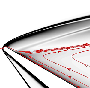
Figure 7 shows the corresponding flow visualisation based on contours of the density gradients for the same case and times  $t=10, 12.07, 13.02, 14.02$ and 14.28 ms corresponding to the last five curves in figure 6. The figure is a close-up of the separated region so that the major flow features are emphasised. In the figure the leading edge and separation shocks are denoted by LES and SS, respectively, and ‘
 $S$’ is the location of separation. Above the separated region, we note compression waves (shocklets) emanating from the shear layer corresponding to number of vortices. The main point to note here is the presence of three secondary vortices, which are formed as the reverse boundary layer (RBL) separates and encounters the primary vortex. The larger vortex ‘1’, which is predominantly on the expansion surface is anchored by the shear layer and the surface by a saddle point (red squares), while the smaller vortices ‘2’ and ‘3’ are located on the compression surface under vortex ‘1’ and under the primary vortex, respectively. We note that from tracking the vortices saddle point that no steady-state solution is reached by the end of the computational time
  $\approx 14.28$ ms. Unsteadiness of secondary vortices has been predicted in the previous numerical studies by Neiland, Sokolov & Shvedchenko (Reference Neiland, Sokolov and Shvedchenko2008) and Shvedchenko (Reference Shvedchenko2009) on compression corner geometry. In the present study, it is shown that unsteadiness can be caused in a leading-edge separation geometry by variations of the angle of incidence.

Figure 7. Flow structure based on the magnitude of the density gradients at  $\alpha =25^{\circ }$:
  $r=1000 \ \mathrm {\mu }$m case with time
  $t$. Results are shown for (a)
  $t = 10$ ms; (b)
  $t=12.07$ ms; (c)
  $t=13.02$ ms; (d)
  $t=14.02$ ms; (e)
  $t=14.28$ ms. Symbols: ‘
 $S$’ is separation, LES is leading-edge shock wave, SS is separation shock wave, 1–3 are the index of the secondary vortices and RBL denotes reverse boundary layer. Red square: saddle point. Here
  $x$ and
  $y$ are Cartesian coordinates in metres. Major streamlines are superposed on the contours.
6. Results and discussion
6.1. Effects of leading-edge bluntness
Figure 8 shows flow features and distributions of wall pressure (8a) and shear stress (8b) with changing nose radius from small (nominally sharp,  $r=15 \ \mathrm {\mu }$m) to the largest bluntness (
 $r=1000 \ \mathrm {\mu }$m) at the baseline angle of
  $\alpha = 30^{\circ }$, including the cases of
  $r=100$ and 500
  $\mathrm {\mu }$m.

Figure 8. Bluntness effects on surface parameters at the baseline incidence of  $\alpha =30^{\circ }$: (a) pressure; (b) shear stress. Legend:
  $r = 15 \ \mathrm {\mu }$m (blue);
  $r = 100 \ \mathrm {\mu }$m (green);
  $r = 500\ \mathrm {\mu }$m (red);
  $r = 1000 \ \mathrm {\mu }$m (grey). Note that
  $p^{*}$ and
  $\tau ^{*}$ are the normalised pressure and shear stress by the free-stream and dynamic pressure, respectively. Note that
  $s^{*}$ is the surface distance and
  $s$ is normalised by the characteristic length,
  $L_e=20$ mm. Here and throughout S is separation and R is reattachment. Insets are the leading-edge region.
Figure 9 shows contours of the density gradient with major streamlines superposed with some salient features of the flow. They cover the full range from nominally sharp to moderate to large bluntness in terms of the criterion suggested by Stollery (Reference Stollery1970) and based on present flow conditions of  $M = 9.66$ and
  $\bar {\chi } = 3.8$. With these stipulations,
  $r=500$
  $\mathrm {\mu }$m approximately demarcates the boundary between ‘large’ and ‘small’ bluntness effects.

Figure 9. Flow structure based on magnitude of the density gradients at  $\alpha =30^{\circ }$. (a)
  $r=15 \ \mathrm {\mu }$m; (b)
  $r=100\ \mathrm {\mu }$m; (c)
  $r=500 \ \mathrm {\mu }$m; (d)
  $r=100 \ \mathrm {\mu }$m. Here and throughout S is separation and R is reattachment, LES is leading-edge shock wave, SS is separation shock wave, TP is triple point, RS is recompression shock wave, ‘1’ is corner vortex and ‘2’ is a secondary wall eddy. Notice that figures (c) and (d) are plotted in difference scales compared with (a) and (b) due to the difference sizes of separation.
  $x$ and
  $y$ are Cartesian coordinates in metres. Major streamlines are superposed on the contours.
Referring to the first two cases  $r = 15\ \mathrm {\mu }$m and 100
  $\mathrm {\mu }$m in figure 9(a,b), they are based on the data given previously in Khraibut et al. (Reference Khraibut, Gai and Neely2019), while the results of the larger
  $r = 500\ \mathrm {\mu }$m and 1000
  $\mathrm {\mu }$m bluntness cases (plots (c) and (d) in the same figure) are based on the grid independence study given above. The main feature to note for the
  $r = 500 \ \mathrm {\mu }$m and
  $r = 1000 \ \mathrm {\mu }$m cases is the occurrence of multiple counter-rotating vortices instead of a large corner vortex embedded within the primary vortex. The vortices appear to grow as the reverse boundary layer encounters the vortical flow and the shear layer is distorted which gives rise to compression waves (shocklets) above the shear layer.
This becomes more obvious when we examine again the insets in figure 8, which show the surface pressure and shear stress for the range of bluntness cases presently studied ( $r=15\unicode{x2013}1000\ \mathrm {\mu }$m). We observe that when the leading-edge radius is increased, the separation point moves towards the curved part of the nose, just upstream of the shoulder for the largest nose radius and the size of separation also increases. This is all consistent with the visualisation based on the global density gradients in figure 9.
It is interesting to note in figure 8(a) that the increase of length of separation relates to the magnitude of the second shear stress minimum just before reattachment, which becomes shallower with increasing bluntness so much so that, for the two larger nose radii, the two minima (just after separation and before reattachment) are almost equal. This shallowing and stretching of the shear stress minimum results in the squeezing and stretching of the primary vortex (see figure 9) with increased bluntness. It is also worth pointing out that the shear stress pattern observed here, as the bluntness is increased, is very similar to the one seen with increasing wall temperature (see Khraibut et al. Reference Khraibut, Gai, Brown and Neely2017), in terms of the length of separation and shallowing of the second shear stress minimum. Note however that increasing nose bluntness seems to have an opposite effect on the fragmentation of vortices compared with increasing wall temperature.
Examining the corresponding pressure distribution (figure 8b), we further note that pressure gradients become substantially milder as reattachment is approached and pushed downstream with an increase in bluntness. This is attributed to the strong favourable pressure gradient induced at the blunt leading edge as the nose radius is increased.
6.2. The entropy layer
For a flat plate with a blunt leading edge and zero angle of incidence in a hypersonic flow, the shock shape can be expressed by the relation (Cheng & Pallone Reference Cheng and Pallone1956) as given earlier in (2.5). This relation was based on the extensive helium data of Hammitt & Bogdonoff (Reference Hammitt and Bogdonoff1956) and its general validity was later confirmed by Cheng et al. (Reference Cheng, Hall, Golian and Hertzberg1961) in their experiments with air. Both Hammitt & Bogdonoff (Reference Hammitt and Bogdonoff1956) and Cheng et al. (Reference Cheng, Hall, Golian and Hertzberg1961) data covered a large range of bluntness Reynolds numbers,  $Re_t$, thus confirming its validity for large and small bluntness values as well as for both adiabatic and cold walls. The equation's applicability for flows at varying angles of incidence, such as the present case, however, needs further justification. Cheng et al. (Reference Cheng, Hall, Golian and Hertzberg1961) and Stollery (Reference Stollery1970) both have shown that in the vicinity of the leading edge, incidence effects, in relation to both heat transfer and pressure, are quite small and only become dominant sufficiently downstream of the leading edge. In the case of a leading-edge separation, that shock shape relation (
 $y_s/t$) should at least be approximately valid, while noting that observations made in these studies were mainly based from measurements and calculations on the windward side, while the flow being discussed here relates to the leeward side (surface
  $AB$ in figure 2).
An estimate of the entropy layer thickness can be made from the shock layer thickness, based on the assumption that the boundary layer thickness is small, which is justified in a leading-edge separation and a cooled wall case. For a blunt flat plate, Oguchi (Reference Oguchi1963) suggests an entropy layer and a shock layer thickness ratio of 0.4 (2.5) so that in the present case, the entropy layer thickness is of the order of 0.76 mm. Figure 10, which shows contours of the density gradients and pressures for nose radii  $r=15$–1000
  $\mathrm {\mu }$m, also shows that the flow is affected by the expansion around the shoulder, but that the overall influence of expansion on shock shape, away from the nose region, is small.

Figure 10. Flow contours of the leading-edge region for  $r=15, 100, 500, 1000$
  $\mathrm {\mu }$m bluntness cases (see top–bottom). Symbols: ‘
 $S$’ is separation, LES is the leading-edge shock wave, SS is the separation shock wave, DSL is the dividing streamline, ‘
 $i$’ is the beginning of shock-viscous interaction. On the left, figures (a–d) are contours of the density gradients and on the right, figures (e–h) are the pressures in pascals. The legend in the pressure figures is scaled to show the range on the leeward side. Here
  $x$ and
  $y$ are Cartesian coordinates in metres. Major streamlines are superposed on the contours.
Figure 10 shows how increasing the leading edge bluntness increases the shock strengths in the leading edge and separation regions (LES and SS, respectively), which is evidenced by the increase of colour intensity of the contours of density gradients (left figures) at these locations with increased bluntness. Note also that in the large  $r=500$ and 1000
  $\mathrm {\mu }$m bluntness cases, the separation moves upstream but remains on the leeward side, which in the figure is noted by movement of the shock-viscous interaction region ‘
 $i$’ on the circumference of the leading edge.
Figure 11 shows the pressure (11a), velocity (11b) and vorticity (11c) profiles at the interaction ‘ $i$’ for the smallest to largest nose radii. In this figure
  $p$ and
  $u_x$ are normalised by the free-stream values, and the vorticity,
  $\omega _z = {{\rm d}u}/{{\rm d} y}-{{\rm d}v}/{{\rm d} x}$, is multiplied by the radius divided by the free-stream velocity. The profiles were taken along the normal as shown in figure 11(c), where the abscissa
  $= 0$ is the wall (subscript ‘
 $w$’) and unity at the edge of the entropy layer (subscript ‘
 $e$’).

Figure 11. Bluntness effects on the interaction profile (‘ $i$’ in figure 10) taken along the wall normal
  $n$: (a) pressure; (b) velocity; (c) vorticity in the
  $z$-direction. Subscripts are consistent with figure 3. Lines:
  $r = 15 \ \mathrm {\mu }$m (blue);
  $r = 100 \ \mathrm {\mu }$m (green);
  $r = 500 \ \mathrm {\mu }$m (red);
  $r = 1000 \ \mathrm {\mu }$m (grey). Coordinates are shown in figure 11(c).
Considering pressure profiles in figure 11(a), first, we note that the pressure stays nearly constant along the entropy layer and only begins to show significant changes with the larger  $r=500$ and 1000
  $\mathrm {\mu }$m bluntness cases. This, in conjunction with the visualisation in figure 10, seems to be caused by the delay in separation in the smaller bluntness cases, away from the leeside expansion and downstream of the bow shock. As a result, the boundary layer is also more developed in the smaller bluntness cases and the pressure range is a lower order than the larger
  $r=500$ and 1000
  $\mathrm {\mu }$m cases.
The corresponding velocity profiles for the same cases are shown in figure 11(b). Here, profiles of the smallest 15 and 100  $\mathrm {\mu }$m bluntness cases show the fuller boundary layer growth prior to separation with its thickness reducing with an increase of bluntness. In the larger bluntness
  $r=500$
  $\mathrm {\mu }$m and 1000
  $\mathrm {\mu }$m cases, that pattern continues so that the boundary layer is very thin as the separation occurs very close to the stagnation point in these two cases and the velocity profile is largely constant across the entropy layer.
In figure 11(c), which shows vorticity profiles for the largest  $r=500$ and 1000
  $\mathrm {\mu }$m bluntness cases, the vorticity drops from a maximum near the surface to a constant at
  $20\unicode{x2013}30\,\%$ of the distance from the wall to the edge of the entropy layer, while the two smaller bluntness cases show these profiles reduce from the maximum value to a constant at about
  $60\,\%$ in the
  $r=15\ \mathrm {\mu }$m bluntness case and
  $40\,\%$ in the
  $r=100$
  $\mathrm {\mu }$m bluntness case. These results are consistent with results from the velocity profiles in figure 11(b) with respect to changes in the boundary layer thickness due to bluntness.
6.3. Effects of incidence on small bluntness
In this section we elucidate the visualisation data obtained from numerical simulations. These visualisations are useful in providing further information on complex flow features of the effects of incidence on separation. Figure 12 shows contours of the density gradient for the three angles of incidence  $\alpha =25^{\circ }$, 30
 $^{\circ }$ and
  $35^{\circ }$ of the nominally sharp
  $r=15 \ \mathrm {\mu }$m case. Streamlines and major flow features, such as length of separation, triple points, shock waves and vortices, are also shown in the figure. In the case of the lowest angle of incidence
  $\alpha =25^{\circ }$ in figure 12(a), there are multiple vortices embedded within the separated region. The primary separation is denoted by locations
  $S$ and
  $R$, while a smaller secondary vortex exists mainly on the expansion surface ‘1’ and eddy ‘2’ emerges from the vertex. With the increase of incidence to
  $\alpha =30^{\circ }$ in figure 12(b), the primary vortex grows and stretches on the compression surface, while stretching the secondary vortex ‘1.’ In this case, corner eddy ‘2’ also amalgamates with vortex ‘1.’ In general, the flow and shocks appear relieved in this case compared with the lower
  $\alpha =25^{\circ }$ incidence. With an additional increase of incidence to
  $\alpha =35^{\circ }$ (figure 12c), still, new features emerge in the flow. Firstly, vortex ‘1’ splits into two smaller eddies disposed on either side of the corner. Secondly, the separating reverse boundary layer experiences a further relief, from the intensity of the contours, while the shocks become weaker and primary separation continues to grow and stretch over the compression surface.

Figure 12. Flow structure variation for  $r=15\ \mathrm {\mu }$m at
  $\alpha$: (a)
  $25^{\circ }$; (b) 30
 $^{\circ }$; (c) 35
 $^{\circ }$. Here and throughout S is separation and R is reattachment, LES is leading-edge shock wave, TP is the triple point, SS is separation shock wave, ‘1 and 2’ are secondary vortices due to the separation of the reverse boundary layer (RBL). Here
  $x$ and
  $y$ are Cartesian coordinates in metres. Major streamlines are superposed on the contours.
In terms of the external flow above the shear layer, both bow and separation shocks reduce in strength with incidence and the effect of that is seen on the movement of separation downstream on the leeside (surface  $AB$ in figure 2). In the smallest incidence case, as a results of separation being closest to the leading edge, the bow and separation shocks are merged but move away from each other with increasing strength of the expansion with an increase of incidence. This is clearly illustrated in figure 13 showing visualisation (based on the magnitude of density gradients and pressures) of the flow in the nose region of the same cases.

Figure 13. Contours of density gradients and pressure near the leading edge for  $r=15\ \mathrm {\mu }$m at various angles of incidence,
  $\alpha$: (a)
  $25^{\circ }$; (b) 30
 $^{\circ }$; (c) 35
 $^{\circ }$. Symbols: ‘
 $S$’ is separation, LES is leading-edge shock wave, SS is separation shock wave and ‘1’ is the corner vortex. The pressure figures on the bottom are in pascals. Here
  $x$ and
  $y$ are Cartesian coordinates in metres. Major streamlines are superposed on the contours.
The effect of incidence on the pressure and shear stress for the same nominally sharp case of 15  $\mathrm {\mu }$m and angles of incidence is illustrated in figures 14(a) and 14(b), respectively. An immediate effect of incidence on the shear stress is in the downstream movement of the separation ‘
 $S$’ and reattachment ‘
 $R$’ with an increase of incidence, also leading to a small overall increase in the length of separation. This confirms the visual results shown in figures 12 and 13. In the reattachment region, in the smallest
  $\alpha =25^{\circ }$ incidence case, also, the shear stress and pressure show two distinct peaks corresponding to the intersection of the leading edge–separation shock with the separation–reattachment shock and expansion, which forms an Edney type VI interaction. With the increase of incidence from
  $30^{\circ }$ to
  $35^{\circ }$, these peaks eventually reduce to a single broad peak in both the pressure and shear stress curves in the
  $35^{\circ }$ incidence case. We also note that the shocks weaken with an increase of incidence. As with the effect of bluntness, pressure gradients in the reattachment also become milder with larger incidence. The shear stress distribution in the neck region, on the other hand, becomes shallower so the second minimum
  $\tau _2$ progressively reduces in magnitude to about a third from
  $\alpha =25^{\circ }$ to
  $35^{\circ }$. Thus, the effect of incidence on the surface parameters is similar to that seen earlier with bluntness.

Figure 14. Incidence effects on surface parameters for the  $r=15 \ \mathrm {\mu }$m case: (a) pressure; (b) shear stress. Legend:
  $\alpha =25^{0}$ (blue);
  $\alpha =30^{0}$ (black);
  $\alpha =35^{0}$ (red). Note that
  $p^{*}$ and
  $\tau ^{*}$ are the normalised pressure and shear stress by the free-stream and dynamic pressure, respectively. Note that
  $s^{*}$ is the surface distance and
  $s$ is normalised by the characteristic length,
  $L_e=20$ mm. Here and throughout S is separation and R is reattachment. Insets are the leading-edge region.
6.4. Effects of incidence on large bluntness
In this section the combined effect of incidence and bluntness are considered for the case with the nose largest radius of 1000  $\mathrm {\mu }$m for the same angles of incidence. In the density gradient contours in figure 15, there are dramatic changes in the flow structure compared with the nominally sharp case. With the
  $25^{\circ }$ incidence (figure 15a), the main separation bubble consists of a main vortex and two other vortices: ‘1’ and ‘2’ near the corner. In this case, an interesting feature to note is the emergence of a saddle point on the crest of vortex ‘1’ with the primary vortex, which as seen in the earlier convergence studies oscillates between a maximum and a minimum.

Figure 15. Variation of flow structure for  $r=1000\ \mathrm {\mu }$m at
  $\alpha$: (a)
  $25^{\circ }$ at
  $t=14.28$ ms; (b) 30
 $^{\circ }$; (c) 35
 $^{\circ }$. Here and throughout S is separation and R is reattachment, LES is leading-edge shock wave, SS is separation shock wave, ‘1–3’ are secondary vortices due to the separation of the reverse boundary layer (RBL). Here
  $x$ and
  $y$ are Cartesian coordinates in metres. Major streamlines are superposed on the contours.
As the incidence increases to  $30^{\circ }$ (figure 15b), a slight increase in the separation length is observed while the shock strengths are reduced. In this case, vortex ‘1’ grows and pushes the primary vortex and vortex ‘2’ is formed below vortex ‘1.’ Compared with the
  $25^{\circ }$ incidence case, the primary vortex at
  $30^{\circ }$ incidence is ‘squashed’ and elongated by the corner vortex ‘1.’ The reverse boundary layer similarly is weaker and dissipates into the primary vortex. With a further increase in incidence to
  $35^{\circ }$, (figure 15c), the separation region is drastically reduced and devoid of compression waves (shocklets) or any other multiple structures. The possible reasons for these flow features become clearer by examining contours of the density gradient and pressure near the leading edge in figure 16.

Figure 16. Contours of density gradients and pressure in the leading-edge region for the largest bluntness case ( $r=1000 \ \mathrm {\mu }$m) at various angles of incidence,
  $\alpha$: (a)
  $25^{\circ }$; (b) 30
 $^{\circ }$; (c) 35
 $^{\circ }$. Symbols: ‘
 $S$’ is separation, LES is leading-edge shock wave, SS is separation shock wave, ‘1’ is the corner vortex. Pressure figures on the bottom are in pascals. Here
  $x$ and
  $y$ are Cartesian coordinates in metres. Major streamlines are superposed on the contours.
For the  $35^{\circ }$ incidence case, we note the separation has moved downstream so there are no secondary vortices or compression waves emanating from the shear layer (figure 16f (top)). Furthermore, with the increase in incidence the overall size of separation is reduced as a result of the combined and cumulative effect of a weakened bow shock and strong shoulder expansion which moves the separation downstream. At the same time, the front stagnation point shifts towards the windward side so that the effect of expansion on the leeward side is strongest. The figure furthermore shows that with the downstream movement of separation at the
  $35^{\circ }$ incidence, the streamline curvature is distinctly concave to the oncoming flow and that the curvature increases with the decrease in incidence.
Figure 17 shows non-dimensional shear stress (17a) and surface pressure (17b) at the three angles of incidence for the largest bluntness case. In the  $\alpha =25^{\circ }$ case, the data are shown at
  $t=14.28$ ms, which is the end of the computational time. Note from the earlier grid independent study (figure 6) the separation length remains steady after
  $t=7.6$ ms while the internal vortices change with time, so that the following discussion is valid. As in the nominally sharp case, we note several notable differences in the shear stress data. Firstly, the smallest
  $25^{\circ }$ and baseline
  $30^{\circ }$ incidence cases are associated with large separated regions with a shallower second shear stress minimum, while the
  $35^{\circ }$ incidence case shows the reverse effect on both parameters. This is similarly reflected in the surface pressures in figure 17(a), wherein the plateau pressure in the separated region after separation is the lowest for the largest
  $35^{\circ }$ incidence and highest for the smallest
  $25^{\circ }$ incidence. As the shock strength reduces with an increase of incidence, we also note that the peaks in the pressure after reattachment become indistinguishable but more pronounced in the shear stress.

Figure 17. Incidence effects on surface parameters for the  $r=1000 \ \mathrm {\mu }$m case: (a) shear stress; (b) pressure. Legend:
  $\alpha =25^{0}$ at
  $t=14.28$ ms (blue);
  $\alpha =30^{0}$ (black);
  $\alpha =35^{0}$ (red). Note that
  $\tau ^{*}$ and
  $p^{*}$ are the normalised shear stress and pressure by the dynamic pressure and free stream, respectively. Note that
  $s^{*}$ is the surface distance and
  $s$ is normalised by the characteristic length,
  $L_e=20$ mm. Here and throughout S is separation and R is reattachment. Insets are the leading-edge region. The grey line is the wall.
In the insets of figures 17(a) and 17(b), the surface pressure and shear stress data in the nose region reflect the previous results. The steep fall in shear stress for the  $25^{\circ }$ and
  $30^{\circ }$ incidence shows that the separation is abrupt, while in the largest
  $35^{\circ }$ incidence it takes place gradually after a boundary layer has sufficiently developed. This corresponds to the reduction seen in the pressure plateau after separation from
  $\approx 17 p_\infty$ in the lowest incidence to
  $\approx 2.6 p_\infty$ in the highest incidence.
6.5. Profiles prior to separation
Transverse profiles of pressure, velocity and vorticity similar to those in figure 11 are shown in figure 18 for the three angles of incidence for the large bluntness case ( $r=1000\ \mathrm {\mu }$m). These profiles are again taken at the beginning of shock-viscous interaction ‘
 $i$’ ahead of separation. In the
  $25^{\circ }$ and
  $30^{\circ }$ incidence cases, as the separation position changes only slightly, profiles of the pressure,
  $p/p_\infty$, velocity,
  $u_x/u_\infty$, and vorticity,
  $w_z r/u_{\infty }$, seem similar, while in the
  $35^{\circ }$ incidence, for which the separation occurs well downstream on the expansion surface, they are quite different.

Figure 18. Flow profiles of pressure (a), velocity (b) and vorticity (c) at the beginning of the interaction ‘ $i$’ and at various angles of incidence in the largest bluntness (
 $r=1000 \ \mathrm {\mu }$m) case:
  $\alpha =25^{\circ }$ (blue);
  $\alpha =30^{\circ }$ (black);
  $\alpha =35^{\circ }$ (red). Wall normal is measured from the wall (subscript ‘
 $o$’) to the edge of the entropy layer (subscript ‘
 $e$’). Parameters are normalised by the edge value of the entropy layer.
The main feature to note in the pressure profiles (figure 18a) is that transverse gradients are present for all incidences, and the lowest pressures in the  $35^{\circ }$ incidence suggests that the effect of expansion is strongest. The velocity profiles (figure 18b), on the other hand, which show the boundary layer growth at each incidence, also show that the boundary layer is fuller (and thicker) in the largest incidence, and the effect of expansion, in the same figure, is seen by an overshoot in the profile, after which the bow shock reduces the velocity at nearly 0.2 of the distance, from the surface to the edge of the entropy layer. The vorticity profiles in figure 18(c) are consistent with velocity profiles in that they are maximum at the surface then approach zero at the edge of the entropy layer. In the
  $35^{\circ }$ incidence there is a corresponding overshoot in the vorticity overshoot at nearly 0.2 of the distance from the surface to the edge of the entropy layer after which the vorticity remains nearly constant.
Figure 19 shows the non-dimensional plateau pressure  $p_p$ in the separated region for the smallest and the largest bluntness (blue diamonds and green circles, respectively) in terms of the parameter
  $K$ for the three angles of incidence, based on (4.2) and (4.3). We have used this parameter to correlate the plateau pressure,
  $p_p$, with an inclined flat plate in the literature as it is a more relevant quantity in the context of leading-edge separation. We first observe with the smallest bluntness, of which the incidence effects are dominant, that
  $K < 1$ and the variation of
  $p_p$ with
  $K$ is nearly linear. In the largest bluntness case, conversely, we note that
  $K > 10$ and the drop in
  $p_p$ is more abrupt so that where the bluntness effect is dominant, as in this case, the changes in
  $K$ with
  $\alpha$ are small. What this shows is that there is a clear demarcation between incidence affects on small and large bluntness. In general, one can say
  $K < 1$ for small and
  $K \gg 1$ for large bluntness.

Figure 19. Variation of non-dimensional plateau pressure (Cheng et al. Reference Cheng, Hall, Golian and Hertzberg1961) with new combined bluntness-incidence parameter  $K$ for the three angles of incidence (
 $\alpha =25^{\circ }\unicode{x2013}35^{\circ }$). Here
  $r=15 \ \mathrm {\mu }$m (blue diamonds) and
  $r=1000 \ \mathrm {\mu }$m (green circles).
6.6. Free interaction, length of separation and shear stress minima
According to Chapman et al. (Reference Chapman, Kuehn and Larson1958), free interaction is a feature of flow wherein the flow is free from ‘direct’ influence of the downstream geometry. However, they state in the same paper that it does not necessarily preclude processes that are not free from ‘indirect’ influence of the downstream flow. As the separation in the present case consists of a primary vortex, which is stretched and pushed downstream, and secondary vortices that are formed by the separation of the reverse boundary layer are pushed upstream so that the separation and reattachment are not entirely independent of each other. It is therefore instructive to compare the different effects on length of separation with the ratio of shear stress minima, which seem to correlate (see tables 3–5). As noted earlier, the leading-edge separation is a limiting case when the distance from the leading edge to separation goes to zero (Délery & Marvin Reference Délery and Marvin1986). Under such circumstances, the boundary layer separates before becoming fully developed and the separation is not a strictly free interaction. This is evident from examining the separation pressures  $p_s^{*}$ (normalised by the free-stream pressure).
Table 3. Effect of wall temperature ( $r=15$
  $\mathrm {\mu }$m;
  $\alpha =30^{\circ }$) on separation pressure, length of separation and ratio of the shear stress minima. Here
  $l_{sep}^{*}$ is normalised by the characteristic length (
 $L_e=20$ mm).

Table 4. Effect of leading-edge nose bluntness ( $T_w=300$ K;
  $\alpha =30^{\circ }$) on separation pressure, length of separation and ratio of the shear stress minima.

Table 5. Effect of incidence ( $T_w=300$ K) on separation pressure, length of separation and ratio of the shear stress minima.

Tables 3–5 show the effects of bluntness, incidence and wall temperature. We note that, for the wall temperature and nose bluntness cases, the separation length increases with an increase of separation pressure while the effect of incidence is quite different. With incidence, in the smallest bluntness cases the separation length reduces with a decrease of separation pressure, and in the largest bluntness case it increases with an increase of  $p_s^{*}$ from
  $\alpha =25^{\circ }$ to 30
 $^{\circ }$, then reduces with a further decrease of
  $p_s^{*}$ at
  $\alpha =35^{\circ }$. The reason for this reversal in the largest bluntness case at
  $\alpha =35^{\circ }$ can be explained when we examine the relationship between the separation length and ratio of shear stress minima for this and the other scenarios in tables 3–5. Note that in these tables,
  $l_{sep}^{*}$ has been normalised by the characteristic length (
 $L_e=20$ mm). We note that when the ratio of the two shear stress minima approaches unity, the length of separation is maximum, and when the ratio is large (i.e. the shear stress distribution is asymmetric), the length of separation is reduced. Once
  $\tau _2/\tau _1$ reaches a minimum, the only possible way for the growth of the length of separation is in the reverse direction. Figure 20 shows the variation of
  $\tau _2/\tau _1$ with
  $l_{sep}^{*}$ for the different effects and it is consistent with these observations. Here, the wall temperature and bluntness effects showed a nonlinear drop in
  $\tau _2/\tau _1$ with an increase in
  $l_{sep}^{*}$, and the smallest bluntness case showed a linear drop with varying incidence. The largest bluntness case showed a similar linear decrease in
  $\tau _2/\tau _1$ with
  $l_{sep}^{*}$, but we note that
  $l_{sep}^{*}$ experiences a reversal of direction for
  $\tau _2/\tau _1 \approx 1$.

Figure 20. Effect of wall temperature, bluntness and incidence on the variation of  $\tau _2/\tau _1$ and length of separation,
  $l_{sep}^{*}$. Black circles:
  $T_w=165, 300, 800, 2770$ K; blue crosses:
  $r=15, 100, 500, 1000$
  $\mathrm {\mu }$m; red diamonds:
  $\alpha =25^{\circ }, 30^{\circ }, 35^{\circ }$ (
 $r=15\ \mathrm {\mu }$m); green triangles:
  $\alpha =25^{\circ }, 30^{\circ }, 35^{\circ }$ (
 $r=1000\ \mathrm {\mu }$m). Here
  $l_{sep}^{*}$ is normalised by the characteristic length (
 $L_e=20$ mm).
7. Conclusions
This paper presents a numerical investigation on the effects of small to large bluntness as well as incidence on leading-edge separation in a laminar hypersonic flow. It has been found that both bluntness of the leading edge and incidence profoundly influence flow separation characteristics, both its size and internal bubble structure. Although leading-edge bluntness and incidence effects on flat plates have been addressed in the past, notably by Cheng et al. (Reference Cheng, Hall, Golian and Hertzberg1961), Kemp (Reference Kemp1968) and Stollery (Reference Stollery1970) and bluntness effects on separation at zero incidence by Holden (Reference Holden1971), the present paper has studied many features of moderate to large nose bluntness and incidence in a hypersonic flow with large separated regions not studied before.
A simplified bluntness and incidence parameter, which is only a function of the Reynolds number based on nose thickness and Mach numbers is suggested. The significance of this parameter is in that it does not rely on the strong shock and plane blast wave analogy. This parameter has also been applied to large separated flows at various angles of incidence and nose radii by comparing the plateau pressures.
Our investigation showed several interesting flow features of hypersonic flows with large separated regions when bluntness is large and the incidence is varied. It was noted that in this particular case the flow was quite unsteady with vigorous movement of the fragmented secondary vortices embedded within the main separation bubble, while the size of separation remained unchanged. It was also noted that these fragmented vortices emanated shocklets in the shear layer and with the increase in incidence both the secondary vortices and strength of the compression waves weakened. And perhaps for the first time, the significance of shear stress minima in describing large separation flows is highlighted.
Acknowledgements
We would like to thank Professor G. Candler of the University of Minnesota for access to US3D. Computer resources were provided by the National Computational Infrastructure (NCI) under the NCMAS Scheme and FD8 project.
Declaration of interests
The authors report no conflict of interest.


