2.1. Quasi-direct numerical simulation set-up

A QDNS of the three-dimensional (3-D) unsteady flow has been performed using the high-performance finite volumes multi-block structured FAST (flexible aerodynamic solver technology) compressible Navier–Stokes solver from ONERA (Péron et al. Reference Péron, Renaud, Mary, Benoit and Terracol2017). The temperature of the wall is imposed at 290 K to reproduce the experimental conditions of Benay et al. (Reference Benay, Chanetz, Mangin, Vandomme and Perraud2006) and Bur & Chanetz (Reference Bur and Chanetz2009). Standard supersonic inflow, outflow and far field conditions are used for the other boundaries. These are characteristics-based boundary conditions that avoid numerical reflections. The computational domain spans over $60^\circ$ in the azimuthal direction with periodic boundary conditions on the sides. This numerical periodicity, which is necessary for the simulation to be affordable, constrains the azimuthal wavenumbers that may exist within the simulated fields, which can only be multiples of 6. To excite convective instabilities, noise is injected at the upstream inlet of the domain (see § 2.2 for details).

The domain is discretised using a structured axisymmetric mesh whose main parameters are presented in table 2. The mesh sizing (presented in appendix C) is such that the flow upstream of the reattachment point is fully resolved with respect to DNS standards. On the flare, where the flow becomes turbulent and the wall-shear-stress is maximum, the sizing of the mesh becomes slightly under-resolved, and corresponds to a highly resolved LES of SBLI (Garnier, Sagaut & Deville Reference Garnier, Sagaut and Deville2002; Teramoto Reference Teramoto2005; Bonne et al. Reference Bonne, Brion, Garnier, Bur, Molton, Sipp and Jacquin2019) rather than a DNS. Therefore, the computation corresponds to a QDNS such as described by Spalart (Reference Spalart2000), since the resolution is in between the typical LES and DNS resolution (Garnier, Adams & Sagaut Reference Garnier, Adams and Sagaut2009; Georgiadis, Rizzetta & Fureby Reference Georgiadis, Rizzetta and Fureby2010).

Table 2. Grid for the QDNS.

A mesh corresponding to a strict DNS in the reattachment region of the flow would require about ten times more grid points, which would drastically increase the computational cost and make the SPOD analysis impossible. However, the dynamics of the reattachment region is not the primary focus of this paper. The goal instead, is to capture the mechanisms of transition, which are driven by coherent structures developing upstream of the reattachment. Therefore, we only need DNS resolution upstream of the transition point and LES resolution downstream, provided the feedback from the downstream region is negligible. This hypothesis was checked by performing a full-fledged DNS over a long enough period of time to converge the mean flow and transition point (but too short for SPOD analysis). Results shown in appendix C indicate that our quasi-DNS trade-off yields an accurate description of both and may therefore be considered appropriate for studying transition, at a fraction of the cost. This conclusion is in line with previous studies (Teramoto Reference Teramoto2005) which already showed that LES may be a satisfactory tool for the study of transition in such flows.

Viscous fluxes are computed using a second-order centred scheme, and convective fluxes are computed using the second-order upwind AUSM(P) scheme proposed by Mary & Sagaut (Reference Mary and Sagaut2002) with a third-order MUSCL reconstruction. The use of an upwind scheme is important in the under-resolved zone of the computation as it maintains the smoothness of the solution by offsetting the energy cascade (Spalart Reference Spalart2000) as is commonly done for monotonically integrated large eddy simulation (MILES). This version of the AUSMP(P) was already successfully used by Bonne et al. (Reference Bonne, Brion, Garnier, Bur, Molton, Sipp and Jacquin2019) in their MILES of an OSBLI case. The time integration is performed via an explicit third-order three-steps Runge–Kutta scheme. The time step is set to $10^{-8}\ \textrm {s}$ to ensure a Courant–Friedrichs–Levy number lower than 0.5 in the whole domain.

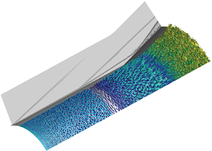
An isosurface of the $Q$-criterion ($Q=9\times 10^{-6}{U^2}/{\delta ^2}$) coupled to a numerical Schlieren visualisation of one snapshot from the DNS is presented in figure 2. It shows the three main regions of interest of the study: the attached boundary layer upstream from the interaction, then the mixing layer between the separation shock and the reattachment point, and finally the reattachment region.

Figure 2. Isosurface of $Q$-criterion ($Q=9\times 10^{-6}{U^2}/{\delta ^2}$) coloured by density and numerical Schlieren visualisation for an instantaneous snapshot of the QDNS.

2.2. Inlet perturbation

As mentioned in § 2.1, noise is added at the inlet of the domain to excite all possible convective instabilities. In several papers (Mayer et al. Reference Mayer, Von Terzi and Fasel2011; Franko & Lele Reference Franko and Lele2013, Reference Franko and Lele2014), the inlet disturbance is chosen in order to excite a particular instability mechanism within the boundary layer. In the present work it was chosen not to decide a priori which mechanism was going to be dominant and to let all of them compete in the simulation. Consequently, a generic spatio-temporally white perturbation has been injected at the inlet, which is able to excite vortical, acoustic and entropic modes. This is reminiscent of the work of Hader & Fasel (Reference Hader and Fasel2018), who injected broadband pressure fluctuations into their numerical simulation to study natural transition mechanisms in hypersonic boundary layers. Note that other choices of generic disturbances may have been considered. The particular receptivity of the chosen noise is studied in the article.

It is worth mentioning that the amplitude of the inlet noise is not a free stream turbulence level and cannot be linked directly to the turbulence level of the R2ch blowdown facility. The article does not aim at reproducing the actual free stream noise of the hypersonic wind tunnel, which is composed of various complex fluctuations (Schneider Reference Schneider2008) with noise radiating from the nozzle and shear layer plus possible perturbations coming from the upstream parts of the blowdown tunnel. Instead, it aims at studying a flow configuration with a generic inlet disturbance, which excites a variety of modes that would develop, compete and interact together.

However, injecting true spatio-temporally white noise raises numerical difficulties as spatial schemes are not designed to work with very short wavelength oscillations (of the order of a few cells). Because of that, high-amplitude white-noise injection requires filtering of the very small wavelength oscillations to avoid numerical instabilities. The present section discusses the effect of the noise amplitude on the flow (including high-amplitude noise). Therefore, it required such filtering, which is performed by a convolution of the disturbance signal by a Gaussian kernel that spans over seven cells in every direction.

Five QDNSs have been performed, each with a different level of filtered inlet noise (the noise levels are presented in figure 3), yielding five mean flows computed by averaging in time and along the azimuthal direction the simulation results. From these mean flows, a bubble length $L_{{sep}}$ can be computed, which gives the results presented in figure 3. The level of noise impacts the transition location and, therefore, influences $L_{{sep}}$ since both the separation and reattachment dynamics strongly depend on the laminar/turbulent nature of the flow. More importantly, these results show that for the appropriate level of inlet perturbation, the QDNS yields results in agreement with the experimental data from Benay et al. (Reference Benay, Chanetz, Mangin, Vandomme and Perraud2006), which validates the present computational parameters. But it also reveals how sensitive the flow is to external noise, which raises the question of the level of perturbation to choose for the present study. We choose not to reproduce the experimental conditions from Benay et al. (Reference Benay, Chanetz, Mangin, Vandomme and Perraud2006). This is mainly because the available experimental results only contain time-averaged data and do not bring any unsteady information on the dynamic of the flow that could be used for comparison. The chosen inlet perturbation involves a lower level of noise, which corresponds to a root mean-squared pressure amplitude of 1.5 % of the free stream value at the inlet and yields $L_{{sep}}\approx 0.5L$ (see figure 3). With such a low level of disturbance, one avoids the numerical stability issues mentioned above, such that the spatial filtering of the inlet perturbation becomes unnecessary. Therefore, to be in the most generic case, all the following results are based on an unfiltered white noise whose amplitude yields the same recirculation length $L_{{sep}}\approx 0.5L$. Quantitative characterisation of the white noise actually injected is given in figure 4: the red curve ($x=0.007$) displays the temporal spectrum of the wall pressure fluctuations a few millimetres downstream from the inlet, showing that the power spectral density is flat as expected. With that precaution, which avoids unnecessary numerical treatment, whatever instabilities growing in the simulations are most likely due to a physical process only. Technical details about the injected noise are presented in appendix B.

Figure 3. Size of the separated region of the mean flow with different levels of filtered noise and experimental value corresponding to the same free stream conditions from Benay et al. (Reference Benay, Chanetz, Mangin, Vandomme and Perraud2006), showing the impact of the disturbance on the topology of the mean flow.

Figure 4. Power spectral density of wall pressure fluctuations at different longitudinal locations of the QDNS.

The impact of the noise on the topology of the flow highlights the importance of boundary layer instabilities, which play a critical role in the transition by selecting and amplifying white noise to trigger secondary instabilities or nonlinear interactions later. In the case presented here, the transition point is located at the reattachment: the incoming boundary layer upstream of the interaction is laminar (incompressible shape factor around $2.7$). At reattachment, the incompressible shape factor is close to $1.5$, characteristic of a turbulent boundary layer. Figure 2 qualitatively shows how the transition process is increasing in intensity as it goes through each studied zone, eventually creating turbulent structures on the flare.

To confirm the assumption that the flow is transitioning at reattachment, figure 5 presents both the intermittency factor and the wall pressure distribution along the geometry. The local intermittency value $\gamma (x)$ represents the probability of being in a turbulent spot at a given time. It is commonly used to describe the transition process (see, for instance, Sandham et al. Reference Sandham, Schülein, Wagner, Willems and Steelant2014). An intermittency factor of 0 thus means that the boundary layer is fully laminar, with no turbulent spot, while a factor of 1 means that the flow is fully turbulent. Everything between 0 and 1 is considered transitional. In the present case, the intermittency factor is computed from spectrograms of wall pressure fluctuations along the geometry, following an idea of Arnal & Juillen (Reference Arnal and Juillen1977). First, a range of ‘laminar’ perturbation frequencies is defined. The presence of a turbulent spot is assumed if fluctuations are detected outside of this range (at higher frequencies). In the present case, it was decided to define the laminar range from 0 Hz up to 600 kHz. These values have been chosen such that the upper limit is more than twice the highest frequency of the common hypersonic boundary layer instabilities (results have shown that the shape of gamma is not impacted by a change of this threshold toward upper frequencies). The results presented in figure 5 show that the intermittency is strictly 0 in the whole attached boundary layer and really close to 0 for most of the separated region (which is characterised by the pressure plateau at $P/P_0=1.6$). In the final part of the mixing layer the intermittency first slightly increases and then brutally reaches 1 at the reattachment (which is characterised by a steep increase in pressure).

Figure 5. Intermittency factor and wall pressure distribution along the geometry showing that the transition is occurring near the reattachment point.

For all the different cases considered in this section, associated with different levels of noise, the transition location obviously changes. But so does the reattachment point, such that eventually, the transition to turbulence always occurs close to the reattachment, and the transition scenario was always the one presented here.

The relation between the recirculation bubble topology and the upstream perturbations has also been documented by Marxen & Rist (Reference Marxen and Rist2010) for incompressible separation. They showed that the transition caused by upstream perturbations leads to the shrinkage of the bubble from both sides. The fact that the flow topology is highly dependent on the level of free stream noise is one of the primary motivations to use the mean flow instead of a base flow for the stability analysis, as it was already advised by Marxen & Rist (Reference Marxen and Rist2010).

2.3. Spectral proper orthogonal decomposition

Convective amplification mechanisms are known to generate coherent structures (Beneddine et al. Reference Beneddine, Sipp, Arnault, Dandois and Lesshafft2016), which may be studied through a SPOD. This variant of the classical proper orthogonal decomposition (POD) was first introduced by Lumley (Reference Lumley1970) and has been widely used by the turbulence community since then (see, for instance, Gudmundsson & Colonius Reference Gudmundsson and Colonius2011). It has been recently studied from a mathematical point of view by Towne, Schmidt & Colonius (Reference Towne, Schmidt and Colonius2018), who showed that it is by construction the optimal decomposition to identify spatio-temporally correlated structures within statistically stationary flow.

To perform the decomposition, one has to first sample snapshots from the simulation, then gather them in $N_{r}$ (possibly overlapping) realisations of the flow. Each realisation contains a temporal sequence of snapshot vectors $(\boldsymbol {s}_{t_0},\boldsymbol {s}_{t_0+{\rm \Delta} t},\dots )$, where the components of $\boldsymbol {s}_{t}$ are the values of the 3-D flow field at time $t$. A direct Fourier transform is then applied both in the temporal and azimuthal direction, giving Fourier mode vectors $\hat {\boldsymbol{\mathsf{S}}}^{k}(\omega ,m)$, where $k$ is the realisation number, $\omega$ the angular frequency and $m$ the azimuthal wavenumber of the mode. Due to the spectral transformation in the azimuthal direction, the vectors $\hat {\boldsymbol{\mathsf{S}}}^{k}(\omega ,m)$ correspond to bi-dimensional fields: they contain complex values associated with each flow variable at each pair $(x,r)$ from the mesh. For a given pair ($\omega$,$m$) of interest, the Fourier modes of all realisations are then stacked in a matrix $\hat {\boldsymbol{\mathsf{X}}}_{\omega ,m}$, which reads as

(2.1)\begin{equation} \hat{\boldsymbol{\mathsf{X}}}_{\omega,m} =\left[ \hat{\boldsymbol{\mathsf{S}}}^{0}(\omega,m), \hat{\boldsymbol{\mathsf{S}}}^{1}(\omega,m), \ldots, \hat{\boldsymbol{\mathsf{S}}}^{N_r-1}(\omega,m) \right]. \end{equation}

This matrix is then processed similarly to a snapshot matrix in a classical space-only POD decomposition: the $i$-th SPOD mode $\boldsymbol {\varPhi }_{\boldsymbol {i}}^{(\omega ,m)}$ can be computed from the $i$-th left singular vector of $\hat {\boldsymbol{\mathsf{X}}}_{\omega ,m}$, which may be computed by solving the eigenproblem associated with the cross-spectral density matrix

(2.2)\begin{equation} \hat{\boldsymbol{\mathsf{X}}}_{\omega,m} \hat{\boldsymbol{\mathsf{X}}}_{\omega,m}^\star {\boldsymbol{\mathsf{Q}}}_{\boldsymbol{\mathsf{e}}} \, \boldsymbol{\varPsi}_{\boldsymbol{i}}^{(\omega,m)} = \lambda_i \boldsymbol{\varPsi}_{\boldsymbol{i}}^{(\omega,m)}, \end{equation}

with ${\boldsymbol{\mathsf{Q}}}_{\boldsymbol{\mathsf{e}}}$ the inner product associated with the energy norm defined by Chu (Reference Chu1965) which is presented in the appendix A. This norm is commonly used in order to describe fluctuation energy in compressible flow (Hanifi, Schmid & Henningson Reference Hanifi, Schmid and Henningson1996; George & Sujith Reference George and Sujith2011; Bugeat et al. Reference Bugeat, Chassaing, Robinet and Sagaut2019) and is more adapted than a simple kinetic energy norm often used for (quasi-)incompressible flows. The SPOD modes are ordered with respect to their contribution to the global dynamics, i.e. $\lambda _0 > \lambda _1 > \lambda _2>\dots$, and for a given pair $(\omega ,m)$, the relative contribution of the $i$-th SPOD mode is measured by the ratio $r_i = \lambda _i / \sum _k \lambda _k$. In the following, we will focus in particular on the leading SPOD mode, and $r_0$ will be systematically specified to quantify how dominant it is compared to the remaining ones.

In practice, the eigenmodes are computed by using the snapshots method of Berkooz, Holmes & Lumley (Reference Berkooz, Holmes and Lumley1993) which is a less costly but equivalent decomposition based on $\hat {\boldsymbol{\mathsf{X}}}_{\omega ,m}^\star {\boldsymbol{\mathsf{Q}}}_{\boldsymbol{\mathsf{e}}} \hat {\boldsymbol{\mathsf{X}}}_{\omega ,m}$ rather than (2.2). This provides the right singular vectors of $\hat {\boldsymbol{\mathsf{X}}}_{\omega ,m}$, from which one can easily retrieve the SPOD modes (see, for instance, Towne et al. (Reference Towne, Schmidt and Colonius2018) for details). The snapshot vector size is also reduced by downsampling the mesh since spatially coherent structures are always significantly bigger than the dissipation scale that needs to be resolved in the QDNS (see table 3). The resulting $i$-th singular vector is a discrete two-dimensional (2-D) field $\boldsymbol {\varPsi }_{\boldsymbol {i}}^{(\omega ,m)}$ corresponding to a slice of the SPOD mode in the azimuthal direction. This framework is well adapted for a spectral study of periodic structures that develop on an axisymmetric geometry such as streamwise vortices. For visualisation purposes, the structure of SPOD modes will be displayed in the present work by showing isocontours of the real part of $\boldsymbol {\varPsi }_{\boldsymbol {i}}^{(\omega ,m)}\,\textrm {e}^{\textrm {i} m\theta }$, which will be called SPOD mode in the captions for conciseness.

Table 3. Numerical parameters for the SPOD.

Note that the spectral resolution in $m$ and $\omega$ of the SPOD is set by the azimuthal span of the computational domain, the temporal length of each realization and the sampling frequency of the snapshots, respectively. These elements, as well as other parameters of the SPOD are specified in table 3. The sampling frequency is set to 200kHz in order to capture the most energetic physical mechanisms in the QDNS, A study using a low-pass filter (not shown here) has been carried out to ensure that this sampling frequency does not yield any noticeable aliasing. The power spectral densities of pressure fluctuations for probes distributed along the wall presented in figure 4 confirm that the transition process comes from a rather low-frequency mechanism and that high-frequency ones (i.e. $f \geqslant 100\ \textrm {kHz}$) are not important in the present context (justifications regarding linear amplification mechanisms will be presented later in § 4.3).

2.4. Fluctuation energy distribution

The matrix formulation used for the SPOD in § 2.3 is convenient to compute the global energy of the fluctuation in the simulation associated to a pair $(\omega ,m)$,

(2.3)\begin{equation} E_{Chu}(\omega,m)=\frac{\textrm{Tr}(\hat{\boldsymbol{\mathsf{X}}}_{\omega,m}^\star{\boldsymbol{\mathsf{Q}}}_{\boldsymbol{\mathsf{e}}} \hat{\boldsymbol{\mathsf{X}}}_{\omega,m})}{N_r}. \end{equation}

Equation (2.3) may be used to produce energy distribution maps that reveal regions in the ($\omega$-$m$)-domain where fluctuations are particularly energetic. A schematic of such a colour map is presented in figure 6, the top right quarter containing the clockwise modes and the bottom right the counter-clockwise modes. Modes along the frequency axis are axisymmetric and modes along the wavenumber axis are steady by construction. As the data from the QDNS are real, the Fourier transformed snapshots display Hermitian symmetry:

(2.4)\begin{equation} \hat{X}_{-\omega,-m}=\overline{\hat{X}_{\omega,m}}. \end{equation}

Because of that, the energy map is symmetric around the origin (i.e. the top right/left quarter is the same as the bottom left/right one). Additionally, as the flow is statistically homogeneous in the azimuthal direction, the clockwise and counter-clockwise modes mirror each other as well. Note that for visualisation purposes, the energy maps are displayed as continuous colour maps. However, the actual values are only defined in discrete pairs ($\omega$-$m$) (that are represented in the background of the maps as dots): $m$ is a multiple of 6 because of the spanwise extent of the domain, and the resolution of the $\omega$ axis is set by the temporal length of the time sequences that are Fourier-transformed (see § 2.3 and table 3).

Figure 6. Schematic of the fluctuation energy distribution map representing the corresponding structures for each zone.

3.1. Resolvent analysis

Global stability analysis is widely used to study the dynamics of fluid flows. In many cases, studying the spectrum of the linearised Navier–Stokes operator gives important information on unstable global modes to understand the origin of unsteady features of the flow. However, as the linearised Navier–Stokes operator is non-normal (i.e. its eigenfunctions are non-orthogonal), initial conditions or external forcings of very low amplitude can trigger high-amplitude fluctuations even when a flow is globally stable. The global resolvent analysis (sometimes called input/output analysis) allows us to study the impact of non-normality of the operator on the amplification of such disturbances. Compared to local approaches commonly used to study transition (such as local stability analysis, parabolised stability equation (PSE) analysis, etc.), no assumption about the parallelism of the flow is required, which makes it perfectly adapted for the study of convective instabilities in the presence of shocks and separation.

Several papers have unveiled the links between resolvent and local stability analyses, and it is now well established that resolvent modes match local stability results in zones where the flow is nearly parallel and dominated by some locally unstable modes. As such, resolvent analyses may be viewed as a generalization of the classical local stability approach, with the difference that it may deal with more complex situations that cannot be factored in by a local stability approach or by PSE (see Sipp & Marquet (Reference Sipp and Marquet2013), Beneddine et al. (Reference Beneddine, Sipp, Arnault, Dandois and Lesshafft2016), Bugeat et al. (Reference Bugeat, Chassaing, Robinet and Sagaut2019) for instance).

In the context of hypersonic boundary layers, the recent work of Bugeat (Reference Bugeat2017), Bugeat et al. (Reference Bugeat, Chassaing, Robinet and Sagaut2019) specifically shows how resolvent modes are related to classical linear stability theory (LST) results from the literature about the well-known modes 1 and 2.

Following the work of Brandt et al. (Reference Brandt, Sipp, Pralits and Marquet2011) and Bugeat et al. (Reference Bugeat, Chassaing, Robinet and Sagaut2019), we can separate the non-normal mechanisms presented in this study into two categories, the ‘convective-type non-normalities’ and the ‘component-type non-normalities’. The former are linked to the advection of perturbations in the mean flow and these are usually referred to as ‘modal’ instabilities in the LST framework. The latter are linked to the transport of mean flow momentum by the perturbations (the ‘lift-up’ effect for example) that would be referred to as non-normal instabilities in the local framework. Note that the vocabulary from the literature is somewhat ambiguous, as ‘modal’ and ‘non-modal’ terms are used differently in the global stability and the local LST frameworks, sometimes to characterise the same underlying physical mechanism. In the following, we focus on global resolvent analysis and use the global stability point of view to refer to the nature of the modes.

Starting from $\boldsymbol {q} =(\rho ,\rho \boldsymbol {u}, \rho E)$ the state vector of the flow and $\boldsymbol {\mathcal {N}}$ the compressible Navier–Stokes operator, the temporal evolution of $\boldsymbol {q}$ is governed by an equation of the form

(3.1)\begin{equation} \frac{\partial \boldsymbol{q}}{\partial t}= \boldsymbol{\mathcal{N}}(\boldsymbol{q}) + \boldsymbol{f}_\textbf{{0}}, \end{equation}

with $\boldsymbol {f}_\textbf {{0}}$ a forcing term corresponding to the injected noise perturbation. By introducing the mean flow $\boldsymbol {\bar {q}_{0}}$ as defined in § 2.2 and ${\boldsymbol{\mathsf{J}}}={\partial \boldsymbol {\mathcal {N}}}/ {\partial \boldsymbol {q}}|_{\boldsymbol {\bar {q}}_\textbf {{0}}}$ the linearisation of $\boldsymbol {{\mathcal {N}}}$ about $\boldsymbol {\bar {q}_0}$, the fluctuation around the mean flow $\boldsymbol {q'}=\boldsymbol {q}-\boldsymbol {\bar {q}}_\textbf {{0}}$ is governed by

(3.2)\begin{equation} \frac{\partial \boldsymbol{q'}}{\partial t} ={\boldsymbol{\mathsf{J}}}\boldsymbol{q'} + \boldsymbol{f}_\textbf{{0}} + \boldsymbol{\mathcal{F}}(\boldsymbol{q'},\bar{\boldsymbol{q}}_\textbf{{0}}), \end{equation}

with $\boldsymbol {\mathcal {F}}(\boldsymbol {q'},\bar {\boldsymbol {q}}_\textbf {{0}}) = \boldsymbol {\mathcal {N}}(\boldsymbol {q}) - {\boldsymbol{\mathsf{J}}}\boldsymbol {q'} - \boldsymbol {f}_\textbf {{0}}$ a term gathering the nonlinear part of the Navier–Stokes operator. Following the formalism of Beneddine et al. (Reference Beneddine, Sipp, Arnault, Dandois and Lesshafft2016), one may then define $\boldsymbol {f'} = \boldsymbol {f}_\textbf {{0}} + \boldsymbol {\mathcal {F}}(\boldsymbol {q'},\bar {\boldsymbol {q}}_\textbf {{0}})$ as a forcing term containing the nonlinear forcing and the injected perturbation such that (3.2) reduces to

(3.3)\begin{equation} \frac{\partial \boldsymbol{q'}}{\partial t} ={\boldsymbol{\mathsf{J}}}\boldsymbol{q'} + \boldsymbol{f'}. \end{equation}

The Fourier transform of (3.3) reads as

(3.4)\begin{equation} \hat{\boldsymbol{q'}}= \mathcal{R}\hat{\boldsymbol{f'}}, \end{equation}

with $\hat {\boldsymbol {f'}}$ and $\hat {\boldsymbol {q'}}$ the Fourier transform of $\boldsymbol {f'}$ and $\boldsymbol {q'}$, respectively, and $\mathcal {R}$ the resolvent operator defined as $\mathcal {R}=(\textrm {i}\omega {\boldsymbol{\mathsf{I}}}-{{\boldsymbol{\mathsf{J}}}})^{-1}$. This compact equation shows that the flow may be seen as an input-output system, where a forcing $\hat {\boldsymbol {f'}}$ generates a response $\hat {\boldsymbol {q'}}$ through the resolvent operator. Then, a resolvent analysis consists in computing for every frequency $\omega$ of interest an optimal forcing $\boldsymbol {\phi }_\textbf {{0}}$ which maximises the gain defined as

(3.5)\begin{equation} \mathcal{G}(\omega) = \frac{ \langle\mathcal{R} \boldsymbol{\phi},\mathcal{R}\boldsymbol{\phi} \rangle_e }{ \langle\boldsymbol{\phi},\boldsymbol{\phi}\rangle }, \end{equation}

where $\langle . , .\rangle _e$ represents the energy of the fluctuation as defined in § 2.4 and $\langle . , . \rangle$ the scalar product associated with the $\mathcal {L}_2$ norm

(3.6)\begin{equation} \langle \boldsymbol{\phi},\boldsymbol{\phi} \rangle = \boldsymbol{\phi}^* {\boldsymbol{\mathsf{Q}}} \boldsymbol{\phi}, \end{equation}

with ${\boldsymbol{\mathsf{Q}}}$ the weight matrix defined in appendix A. The optimal forcing and the associated gain are given by the dominant right singular vector and dominant singular value of $\mathcal {R}$, and they may be computed by solving

(3.7)\begin{equation} \mathcal{R}^* {\boldsymbol{\mathsf{Q}}}_{\boldsymbol{\mathsf{e}}} \mathcal{R} \boldsymbol{\phi}_{\boldsymbol{i}} = \mu_i^2 {\boldsymbol{\mathsf{Q}}} \boldsymbol{\phi}_{\boldsymbol{i}}. \end{equation}

The highest eigenvalue $\mu _0^2$ of (3.7) is the optimal gain, the corresponding eigenvector $\boldsymbol {\phi }_\textbf {{0}}$ is the optimal forcing. These quantities are functions of the frequency $\omega$. Additionally, as shown in § 3.2, one may perform a Fourier transform of (3.2) in the azimuthal direction such that the gain and optimal forcing are not only functions of $\omega$, but also functions of the azimuthal wavenumber $m$.

Computing lower-magnitude eigenvalues $\mu _{i\geqslant 1}^2$ of (3.7) gives sub-optimal forcings $\boldsymbol {\phi }_{\boldsymbol {i}\geqslant \textbf {1}}$. After normalization, these forcings yield an orthonormal basis of the forcing space, i.e. $\langle \boldsymbol {\phi }_{\boldsymbol {i}},\boldsymbol {\phi }_{\boldsymbol {j}} \rangle = \delta _{ij}$. The optimal responses given by $\boldsymbol {\psi }_{\boldsymbol {i}}=\mathcal {R}\boldsymbol {\phi }_{\boldsymbol {i}}/|| \mathcal {R}\boldsymbol {\phi }_{\boldsymbol {i}}||_e$ gives a similar basis of the response space, and (3.4) may then be decomposed as

(3.8)\begin{equation} \hat{\boldsymbol{q'}} =\boldsymbol{\psi}_\textbf{{0}}\mu_0 \langle\boldsymbol{\phi}_\textbf{{0}}, \hat{\boldsymbol{f'}}\rangle + \sum_{i\geqslant 1} \boldsymbol{\psi}_{\boldsymbol{i}} \mu_i \langle\boldsymbol{\phi}_{\boldsymbol{i}}, \hat{\boldsymbol{f'}}\rangle. \end{equation}

Physically, when there exists one strong convective instability mechanism within the flow (such as first or second mode instabilities), the optimal gain becomes very high, and the resolvent analysis yields $\mu _0\gg \mu _{i\geqslant 1}$ (see Beneddine et al. Reference Beneddine, Sipp, Arnault, Dandois and Lesshafft2016). When this occurs, the first term on the right-hand-side of (3.8) is expected to be dominant, as long as the noise contained in $\hat {\boldsymbol {f'}}$ does not preferentially excite a suboptimal forcing in a way that shifts the dominance (which was never observed in the present study). Then, $\hat {\boldsymbol {q'}}$ is going to be dominated by the first optimal response $\boldsymbol {\psi }_\textbf {{0}}$ as a result of this strong linear amplification mechanism. Therefore, the resolvent analysis may explain the appearance of coherent structures, and as such, it is an important tool to confront with SPOD analyses.

However, $\hat {\boldsymbol {f'}}$ may project better onto $\boldsymbol {\phi }_\textbf {{0}}$ for some given values of $(m,\omega )$. This may be investigated by introducing the coefficient $c_0 = \mu _0^2 |\langle \boldsymbol {\phi }_\textbf {{0}},\hat {\boldsymbol {f'}}\rangle |^2$, which represents the combination of two mechanisms: the ability of the linear operator to optimally amplify a certain type of structure (through $\mu _0$) and the strength of the excitation of this mechanism by $\hat {\boldsymbol {f'}}$, which contains both the injected noise and the nonlinear terms. Situations where $E_{Chu}(\omega ,m)$ is high while the dominant amplification mechanism is weak (i.e. $\mu _0^2(\omega ,m)$ is small) may be explained by receptivity processes that are accounted for by $c_0(\omega ,m)$. In general, in the context of strong nonlinear interaction and no dominant linear instability mechanism, $c_0(\omega ,m)$ is not expected to match $E_{Chu}(\omega ,m)$ since there is no reason for the forcing term $\hat {\boldsymbol {f'}}$ to specifically excite a given linear mechanism. However, if $c_0(\omega ,m)$ matches $E_{Chu}(\omega ,m)$ then, for this particular pair $(\omega ,m)$, the forcing term projects well onto $\boldsymbol {\phi }_\textbf {{0}}$ such that high-energy structures stem from a weak (but strongly excited) linear mechanism. As shown in the following, such a situation where the nonlinearities excite a very specific linear amplification mechanism is central for the transition scenario of the studied flow configuration.

It is also interesting to discriminate the contribution of the injected noise from the contribution of the nonlinear terms in the receptivity processes. To do so, one may simply compute $c_r$, which is defined in the same way as $c_0$ but with a scalar product spatially restricted to the stencil of the injection plane of the noise (i.e. the support of the forcing term). If $c_r$ is close to $c_0$, the receptivity is linked to the nature of the noise alone. Otherwise, the receptivity of the nonlinear terms also comes into play.

In order to preserve the stochastic framework introduced in § 2.3 and to conform with the SPOD approach, the actual computation of $c_{0}$ in the following is $c_{0} = \mu _0^2 E[|\langle \boldsymbol {\phi }_\textbf {{0}},\hat {\boldsymbol {f'}}\rangle |^2]$, where $E[.]$ is the expected value estimated from an average of values computed for several realisations (using the same time sequences as for the SPOD analysis described in § 2.3), $\hat {\boldsymbol {f'}}$ being computed as $\mathcal {R}^{-1}\hat {\boldsymbol {q'}}$.

Note that it is possible to localise the resolvent analysis to a given region of the flow by setting all coefficients of ${\boldsymbol{\mathsf{Q}}}_{\boldsymbol{\mathsf{e}}}$ associated with cells outside of this region to zero. The gain is then defined as the maximal energy restrained to this specific zone, and as such, the response is constrained in space (but the forcing is not). This approach is used in the following to study coherent structures in specific domains of the flow.

3.2. Azimuthal decomposition of the resolvent analysis

The computation of the resolvent operator requires the Jacobian matrix. Following the procedure described by Beneddine (Reference Beneddine2017), ${\boldsymbol{\mathsf{J}}}$ is obtained by a finite-differences linearisation of the discrete equations implemented in FAST. The largest eigenvalues of (3.7) may then be solved using the Arnoldi algorithm coupled with an LU solver for the inversion phase (using ARPACK Lehoucq, Sorensen & Yang (Reference Lehoucq, Sorensen and Yang1998) and MUMPS Amestoy et al. (Reference Amestoy, Duff, L'Excellent and Koster2001)). Unfortunately, given the size of the matrices involved, the computational cost of this strategy is not affordable. But since the mean flow is axisymmetric and the mesh is homogeneous in the azimuthal direction, the Jacobian operator may be rearranged in a block-diagonal form as proposed by Schmid, de Pando & Peake (Reference Schmid, de Pando and Peake2017) to make the computation significantly cheaper. This cost-reduction method, which has also been used in Paladini et al. (Reference Paladini, Beneddine, Dandois, Sipp and Robinet2019), is briefly presented below.

Since the solver FAST works internally with Cartesian coordinates, one has to first carry out a transformation to cylindrical coordinates to retrieve the axisymmetry of the flow using the following relation

(3.9)\begin{equation} \left( \begin{array}{@{}c@{}} \rho \\ \rho {u_x}\\ \rho {u_r}\\ \rho u_\theta \\ \rho E \end{array} \right) = \left[ \begin{array}{@{}ccccc@{}} 1 & 0 & 0 & 0 & 0 \\ 0 & 1 & 0 & 0 & 0 \\ 0 & 0 & \cos(\theta) & \sin(\theta) & 0 \\ 0 & 0 & -\sin(\theta) & \cos(\theta) & 0 \\ 0 & 0 & 0 & 0 & 1 \end{array} \right] \left(\begin{array}{@{}c@{}} \rho \\ \rho {u_x}\\ \rho {u_y}\\ \rho u_z \\ \rho E \end{array} \right). \end{equation}

Under appropriate indexing of the degrees of freedom, the Jacobian operator can then be rearranged into the block-circulant form

(3.10)\begin{equation} {\boldsymbol{\mathsf{J}}} = \left[\begin{array}{@{}ccccc@{}} {\boldsymbol{\mathsf{A}}}_0 & {\boldsymbol{\mathsf{A}}}_1 & \cdots & {\boldsymbol{\mathsf{A}}}_{n-2} & {\boldsymbol{\mathsf{A}}}_{n-1}\\ {\boldsymbol{\mathsf{A}}}_{n-1} & {\boldsymbol{\mathsf{A}}}_0 & \cdots & {\boldsymbol{\mathsf{A}}}_{n-3} & {\boldsymbol{\mathsf{A}}}_{n-2}\\ {\boldsymbol{\mathsf{A}}}_{n-2} & {\boldsymbol{\mathsf{A}}}_{n-1} & \cdots & {\boldsymbol{\mathsf{A}}}_{n-4} & {\boldsymbol{\mathsf{A}}}_{n-3}\\ \vdots & \vdots & \vdots & \vdots & \vdots \\ {\boldsymbol{\mathsf{A}}}_1 & {\boldsymbol{\mathsf{A}}}_2 & \cdots & {\boldsymbol{\mathsf{A}}}_{n-1} & {\boldsymbol{\mathsf{A}}}_{0} \end{array} \right] , \end{equation}

where each line of blocks corresponds to a given azimuthal slice of the mesh and the block matrices ${\boldsymbol{\mathsf{A}}}_0, \ldots , {\boldsymbol{\mathsf{A}}}_{n-1}$ have a size corresponding to such a slice (the size of a 2-D problem). The block-circulant nature of the matrix comes from the numerical and physical equivalence of all azimuthal slices of the mean flow, which cannot be distinguished from one another. As shown by Schmid et al. (Reference Schmid, de Pando and Peake2017), this block-circulant matrix can then be transformed into a block-diagonal matrix

(3.11)\begin{equation} \tilde{{\boldsymbol{\mathsf{J}}}} = \left[ \begin{array}{@{}ccccc@{}} \tilde{{\boldsymbol{\mathsf{A}}}}_0 & & & & \\ & {\tilde{{\boldsymbol{\mathsf{A}}}}}_1 & & & \\ & & \ddots & & \ \\ & & & & \tilde{{\boldsymbol{\mathsf{A}}}}_{n-1} \end{array} \right], \end{equation}

with

(3.12)\begin{equation} \tilde{{\boldsymbol{\mathsf{A}}}}_m = {\boldsymbol{\mathsf{A}}}_0 + \rho_m {\boldsymbol{\mathsf{A}}}_1 + \rho_m^2 {\boldsymbol{\mathsf{A}}}_2 + \cdots+ \rho_m^{n-1} {\boldsymbol{\mathsf{A}}}_{n-1}, \end{equation}

and $\rho _m=\textrm {e}^{{\textrm {i} 2 {\rm \pi}m}/{n}}$ corresponding to an $m$-root of unity.

Then, the analysis of the global 3-D resolvent may be done by performing $n$ smaller resolvent analyses by successively considering for $m=0,\dots ,n-1$ the operator

(3.13)\begin{equation} \tilde{\mathcal{R}}(m,\omega)=(\textrm{i}{\boldsymbol{\mathsf{I}}}\omega-{\tilde{{\boldsymbol{\mathsf{A}}}}}_m)^{-1}. \end{equation}

For each value of $m$, the 3-D optimal forcing and response, denoted as $\boldsymbol {\phi }_m$ and $\boldsymbol {\psi }_m$, respectively, are the singular vectors of $\mathcal {R}$ and can be computed from those of $\tilde {\mathcal {R}}$: $\tilde {\boldsymbol {\phi }}_m,\tilde {\boldsymbol {\psi }}_m$ as

(3.14a,b)\begin{equation} \boldsymbol{\phi}_m = \left( \begin{array}{@{}c@{}} \tilde{\boldsymbol{\phi}}_m \\ \rho_m \tilde{\boldsymbol{\phi}}_m\\ \rho_m^2 \tilde{\boldsymbol{\phi}}_m\ \\ \vdots \\ \rho_m^{n-1} \tilde{\boldsymbol{\phi}}_m \\ \end{array} \right),\quad\boldsymbol{\psi}_m = \left( \begin{array}{@{}c@{}} \tilde{\boldsymbol{\psi}}_m \\ \rho_m \tilde{\boldsymbol{\psi}}_m\\ \rho_m^2 \tilde{\boldsymbol{\psi}}_m\ \\ \vdots \\ \rho_m^{n-1} \tilde{\boldsymbol{\psi}}_m \end{array} \right). \end{equation}

This shows that $m$ is actually the azimuthal wavenumber of the resolvent mode. With this formulation, the resolvent operator does not only depend on the frequency but also $m$. This leads to an analysis in the $(\omega , m)$-domain that allows direct comparison of the resolvent gain with the energy map (see § 2.4). For that reason, resolvent analyses are performed for values of $m$ corresponding to multiples of 6 to be consistent with the DNS, and gain values are displayed for a $(\omega , m)$-domain encompassing that of the energy maps (including negative values of $m$ and $\omega$). Thus, the interpretation of the map is the same as that presented in figure 6 and § 2.4.