


1 Introduction
A charged drop of radius  $a$ suspended in a medium with electrical permittivity
  $\unicode[STIX]{x1D716}_{e}$ undergoes an instability when the total charge on the drop exceeds a critical value of
  $Q_{c}=8\unicode[STIX]{x03C0}\sqrt{\unicode[STIX]{x1D6FE}a^{3}\unicode[STIX]{x1D716}_{e}}$, where
  $\unicode[STIX]{x1D6FE}$ is the surface tension of the drop (Rayleigh 1882). This is termed the Rayleigh instability, which is believed to be responsible for the breakup of raindrops in thunderstorms, the formation of sub-nanometre droplets in electrosprays and the generation of ions in ion-mass spectrometry (Fenn et al. Reference Fenn, Mann, Meng, Wong and Whitehouse1989; Rosell-Llompart & De La Mora Reference Rosell-Llompart and De La Mora1994). This instability occurs when the repulsive Coulombic force overcomes the restoring surface tension force. An infinitesimal quadrupolar shape perturbation (the second Legendre mode) on a spherical drop charged beyond
  $Q_{c}$ is known to be the most unstable mode (Tsamopoulos, Akylas & Brown Reference Tsamopoulos, Akylas and Brown1985; Basaran & Scriven Reference Basaran and Scriven1989; Thaokar & Deshmukh Reference Thaokar and Deshmukh2010). Although the Rayleigh limit predicts the point of onset of instability, it leaves the details of the break up pathway completely unspecified. To predict the Rayleigh fission process various theoretical models using the energy minimization method were proposed in the literature (Ryce & Patriarche Reference Ryce and Patriarche1965; Pfeifer & Hendricks Reference Pfeifer and Hendricks1967; Bailey Reference Bailey1974; Roth & Kelly Reference Roth and Kelly1983; Elghazaly & Castle Reference Elghazaly and Castle1987). However, these simplistic models were based on several assumptions, such as a charged drop undergoing binary division or disrupting into
  $n$ identical progeny droplets, the energy of the system being conserved before and after the breakup event, the charge on the mother drop being distributed uniformly to the
  $n$ progeny droplets. The models compare the initial and final states of the system and ignore the fluid dynamics, whereby the pathway cannot be explained in this formalism. Thus, these models could not correctly capture the complex breakup pathway of a critically charged drop.
The inherent complexity present in the breakup mechanisms was demonstrated only recently through systematic experiments on a levitated charged drop in a quadrupolar trap (Duft et al. Reference Duft, Achtzehn, Müller, Huber and Leisner2003; Giglio et al. Reference Giglio, Gervais, Rangama, Manil, Huber, Duft, Müller, Leisner and Guet2008). These experiments indicated that, above its Rayleigh limit, a charged drop gradually deforms into the shape of a prolate spheroid, elongating further to form sharp conical tips, wherefrom a jet emerges within a very short time. These jets further disintegrate into a cloud of smaller daughter droplets which eventually take away a significant fraction (20 %–50 %) of the original charge, although the associated mass loss is small (0.1 %–1 %) (Doyle, Moffett & Vonnegut Reference Doyle, Moffett and Vonnegut1964; Abbas & Latham Reference Abbas and Latham1967; Roulleau & Desbois Reference Roulleau and Desbois1972; Richardson, Pigg & Hightower Reference Richardson, Pigg and Hightower1989; Taflin, Ward & Davis Reference Taflin, Ward and Davis1989; Duft et al. Reference Duft, Achtzehn, Müller, Huber and Leisner2003). The size and charge on the daughter droplets thus formed are important since they determine whether the progenies can undergo further breakup or not. In this paper, we focus on providing a model to explain the observed breakup pathway and estimate the size and charge on the daughter droplets.
The Rayleigh fission process of an isolated charged drop is generally modelled under the assumption of a perfectly conducting (PC) liquid drop in which the charges are distributed uniformly on its equipotential surface. The flow equations are solved numerically using the boundary element method (BEM) either in the viscous flow limit (Betelú et al. Reference Betelú, Fontelos, Kindelán and Vantzos2006) or in the potential flow limit (Burton & Taborek Reference Burton and Taborek2011). Both these studies show that the charged drop deforms initially into the shape of a spheroid, progressively deforming into an elongated object with sharp conical tips, whereafter it undergoes a numerical singularity. The results in the viscous flow limit indicate that the capillary stresses at the sharp tips become subdominant and a balance of the viscous and the electric stresses leads to the formation of a dynamic cone angle of approximately 25°. In contrast, the simulations for the potential flow limit yield a cone angle of approximately 49. 3°, coincidentally close to the classical equilibrium angle of the Taylor cone derived from static considerations. Actual experimental images show a cone angle of 30°, indicating significant viscous effects (Giglio et al. Reference Giglio, Gervais, Rangama, Manil, Huber, Duft, Müller, Leisner and Guet2008). Furthermore, the PC model was also used for predicting fractional charge loss of approximately 39 % (Gawande, Mayya & Thaokar Reference Gawande, Mayya and Thaokar2017) assuming negligible mass loss.
To proceed beyond singularity within the framework of the PC model and predict ejection, Garzon, Gray & Sethian (Reference Garzon, Gray and Sethian2014) performed BEM simulations coupled with a level set technique for inviscid drops. Although the model could predict the formation of daughter droplets, the ejection occurred from protrusions, whose lengths were far smaller (1/5th of the droplet diameter), in contrast to the experimental observation of long (3 times the drop diameter) jets (Duft et al. Reference Duft, Achtzehn, Müller, Huber and Leisner2003; Giglio et al. Reference Giglio, Gervais, Rangama, Manil, Huber, Duft, Müller, Leisner and Guet2008). Besides, in view of the absence of viscosity, the protrusions observed in these numerical studies were likely to be artefacts of inertial excursions rather than due to sustained axial momentum exerted by tangential stresses necessarily required for jet formation. Considering these, the PC model fails to predict the jet formation and one needs to look for alternative mechanisms to explain the complex pathway of break up seen in the experiments. This indicates that it is necessary to consider a high but finite value of conductivity of the drop while solving the Rayleigh breakup problem.
Taylor (Reference Taylor1966) suggested the leaky dielectric model for systems where the charged double layer thickness is much smaller than the other length scales in the system. When the droplet and the surrounding fluid both are weakly conducting, the difference in the electric current inside and outside the droplet gives rise to a surface charge distribution. Thus, the drop surface is acted upon by tangential electric stresses along with normal stresses. These tangential stresses are balanced by viscous stresses which result in the flow inside the droplet. The direction of the flow depends on the electrical properties, such as permittivities and conductivities of the drop and the surrounding medium, which decide whether the droplet will deform into a prolate or oblate shape (Melcher & Taylor Reference Melcher and Taylor1969; Saville Reference Saville1997). This model is widely used in the literature for the numerical prediction of steady state deformations as well as breakup modes of low conducting droplets under an applied electric field assuming the Stokes flow limit (Sherwood Reference Sherwood1988; Basaran et al. Reference Basaran, Patzek, Benner and Scriven1995; Dubash & Mestel Reference Dubash and Mestel2007; Lac & Homsy Reference Lac and Homsy2007; Supeene, Koch & Bhattacharjee Reference Supeene, Koch and Bhattacharjee2008; Deshmukh & Thaokar Reference Deshmukh and Thaokar2013; Karyappa, Deshmukh & Thaokar Reference Karyappa, Deshmukh and Thaokar2014). Although these studies have shown the effect of tangential stresses on the drop deformation and breakup, the effect of charge convection is neglected, assuming instantaneous surface charge relaxation as compared to the deformation (hydrodynamic) time.
The surface charge convection, however, cannot be always ignored when the electrohydrodynamic time scale is of the same order as the charge relaxation time. For the case of viscous droplets deforming under an applied electric field, in the leaky dielectric framework, Feng (Reference Feng1999) accounted for the charge convection effect to predict the steady prolate and oblate deformations and reported that the oblate deformations are suppressed while prolate deformations are enhanced when the charge convection is considered. This observation is further confirmed by Lanauze, Walker & Khair (Reference Lanauze, Walker and Khair2015) and Das & Saintillan (Reference Das and Saintillan2017) considering an unsteady state charge dynamics equation that accounts for the effects of convection of charges and dilatation of the drop interface on the temporal evolution of surface charge density. These studies also indicated that when surface charge convection effects are considered, not only the steady state deformations but also the temporal evolution of the drops are altered. The analysis is further extended to predict the breakup of prolate drops where the electric Reynolds number (a measure of the relative importance of the charge relaxation and hydrodynamic time scales) is observed to significantly affect the modes of breakup of the prolate drops (Sengupta, Walker & Khair Reference Sengupta, Walker and Khair2017). A similar model with an outside medium that is a perfect dielectric is used by Collins et al. (Reference Collins, Jones, Harris and Basaran2008, Reference Collins, Sambath, Harris and Basaran2013), who demonstrated that the charge dynamics and the viscous stresses are necessary for the jet formation in the study of the breakup of uncharged oil drops under strong applied electric fields.
Recently, Gañán-Calvo et al. (Reference Gañán-Calvo, López-Herrera, Rebollo-Muñoz and Montanero2016) and Pillai et al. (Reference Pillai, Berry, Harvie and Davidson2016) studied the electrokinetic effects on the ejection of jet and progeny from the drops under electric fields using the volume of fluid approach by respectively ignoring and considering the thermal energy of the ions. Both these analyses are carried out for low to moderate Ohnesorge number ( $Oh=\unicode[STIX]{x1D707}_{i}/\sqrt{\unicode[STIX]{x1D70C}_{i}a\unicode[STIX]{x1D6FE}}\leqslant 10$) values. These studies indicated that, near the cone–jet transition, the charge transport to the surface of the drop from the bulk is limited by ion mobility and thus the electrokinetic effects significantly modify the transient drop dynamics. However, it is observed that the importance of the electrokinetic effects reduces for higher
  $Oh$ values and can become redundant in the large
  $Oh$ limit (i.e. for highly viscous drops) (Pillai et al. Reference Pillai, Berry, Harvie and Davidson2016). A detailed physical discussion on electrokinetic effects and the applicability of the leaky dielectric model in the context of a cone–jet electrospray system was recently reviewed in Ganán-Calvo et al. (Reference Ganán-Calvo, López-Herrera, Herrada, Ramos and Montanero2018).
In the Rayleigh breakup of a charged drop, the perfect conductor model fairly predicts the drop deformation until the formation of the cone (Betelú et al. Reference Betelú, Fontelos, Kindelán and Vantzos2006; Giglio et al. Reference Giglio, Gervais, Rangama, Manil, Huber, Duft, Müller, Leisner and Guet2008; Gawande et al. Reference Gawande, Mayya and Thaokar2017; Singh et al. Reference Singh, Gawande, Mayya and Thaokar2019b). Up to this stage, the bulk charges are indeed zero. At the time of onset of jet ejection at the tip of the cones, the bulk charge conductivity effect could manifest as a charge depletion layer at the interface. In the present work, the charge near the interface, which is spread into the bulk as volume charge density, is volume averaged and expressed as a surface charge. The surface charge density variations are then considered accurately through the surface charge dynamics model. Thus, the model is accurate when the bulk charge depletion layer is smaller than other length scales in the problem such that volume averaging remains meaningful.
In this work, for  $Oh\rightarrow \infty$, we therefore ignore the dynamics in bulk conduction and apply the leaky dielectric model to the case of Rayleigh break up of a charged drop (in the absence of any external electric field). We consider the drop has high but finite conductivity which involves faster dynamics and high electrical stresses due to high permittivity ratios as compared to oil drops. We call this a finite conductivity (FC) model as the drop needs to support high charge to undergo Rayleigh breakup and the outer medium considered is perfectly dielectric. Thus, the total charge on the drop is conserved throughout the breakup process. The main objective of this work is to explore the mechanism involved in the formation of jet and progeny during the Rayleigh breakup of a charged drop. It should be noted that, in the presence of an external electric field, the drop deformation consistently increases with the applied field, while in the Rayleigh breakup of a charged droplet considered in this work, the droplet is rendered unstable only when the charge increases beyond a critical limit and spherical symmetry is perturbed by a small dipolar perturbation.
2 Problem formulation
The problem is solved numerically by considering an electrically charged drop of a conducting liquid of viscosity  $\unicode[STIX]{x1D707}_{i}$, permittivity,
  $\unicode[STIX]{x1D716}_{i}$ and conductivity
  $\unicode[STIX]{x1D70E}_{i}$ suspended in a perfectly dielectric Newtonian fluid medium of viscosity
  $\unicode[STIX]{x1D707}_{e}$ with a permittivity,
  $\unicode[STIX]{x1D716}_{e}$. We consider the hydrodynamics in the Stokes flow limit, where
  $Oh$ is large and the electrokinetic effects are neglected such that
  $a>\unicode[STIX]{x1D6FC}_{D}$, where
  $\unicode[STIX]{x1D6FC}_{D}$ is the Debye layer thickness (Gañán-Calvo et al. Reference Gañán-Calvo, López-Herrera, Rebollo-Muñoz and Montanero2016; Pillai et al. Reference Pillai, Berry, Harvie and Davidson2016). Thus, this limit could be considered for the breakup of droplets of sizes of the order of their viscous length scales (
 $\unicode[STIX]{x1D707}_{i}^{2}/(\unicode[STIX]{x1D70C}\unicode[STIX]{x1D6FE})$) or smaller, but greater than
  $\unicode[STIX]{x1D6FC}_{D}$. The governing equations for the flow field are then given by
 $$\begin{eqnarray}\displaystyle & \tilde{\unicode[STIX]{x1D735}}\boldsymbol{\cdot }\tilde{\boldsymbol{v}}_{i,e}=0, & \displaystyle\end{eqnarray}$$
 $$\begin{eqnarray}\displaystyle & -\tilde{\unicode[STIX]{x1D735}}\tilde{p}_{i,e}+\unicode[STIX]{x1D707}_{i}\tilde{\unicode[STIX]{x1D6FB}}^{2}\tilde{\boldsymbol{v}}_{i,e}=0. & \displaystyle\end{eqnarray}$$
 Here, the subscripts  $i$ and
  $e$ represent the parameters corresponding to the drop and the external medium respectively and the external medium is considered to be air. The electric potential on the surface of the drop due to the presence of surface charge is denoted by
  $(\tilde{\unicode[STIX]{x1D719}})$ and is assumed to follow
 $$\begin{eqnarray}\tilde{\unicode[STIX]{x1D735}}^{2}\tilde{\unicode[STIX]{x1D719}}_{i,e}=0.\end{eqnarray}$$
 The electric field is thus expressed as  $\tilde{\boldsymbol{E}}_{i,e}=-\tilde{\unicode[STIX]{x1D735}}(\tilde{\unicode[STIX]{x1D719}}_{i,e})$.
The dimensional quantities are indicated by a tilde and non-dimensional quantities are without a tilde. The non-dimensional parameters used in this problem are as follows: length scales are of the order of the initial radius  $a$ of the spherical drop. The time is non-dimensionalized by the hydrodynamic time scale,
  $t_{h}=\unicode[STIX]{x1D707}_{i}a/\unicode[STIX]{x1D6FE}$, the velocity by
  $\unicode[STIX]{x1D6FE}/\unicode[STIX]{x1D707}_{i}$, the surface charge density
  $\tilde{q}$ by
  $\sqrt{\unicode[STIX]{x1D6FE}\unicode[STIX]{x1D716}_{e}/a}$ and the electric field by
  $\sqrt{\unicode[STIX]{x1D6FE}/a\unicode[STIX]{x1D716}_{e}}$. The total surface charge is non-dimensionalized by
  $\sqrt{\unicode[STIX]{x1D6FE}a^{3}\unicode[STIX]{x1D716}_{e}}$ such that the non-dimensional Rayleigh charge is
  $8\unicode[STIX]{x03C0}$. The electrostatic and Stokes equations are solved using the axisymmetric boundary integral method, using well-established methodologies (Deshmukh & Thaokar Reference Deshmukh and Thaokar2012; Lanauze et al. Reference Lanauze, Walker and Khair2015; Gawande et al. Reference Gawande, Mayya and Thaokar2017).
For a finitely conducting charged drop, the electric boundary conditions at the interface in the scaled variables can be written as  $E_{ne}-SE_{ni}=q$,
  $E_{t_{e}}=E_{t_{i}}$. Thus the boundary integral equation for the electric field calculation is given by
 $$\begin{eqnarray}\displaystyle & & \displaystyle \frac{(S+1)}{2S}E_{n_{e}}(\boldsymbol{r}_{s})+\frac{1}{4\unicode[STIX]{x03C0}}\frac{(S-1)}{S}\int \boldsymbol{n}\boldsymbol{\cdot }\unicode[STIX]{x1D735}\boldsymbol{G}^{e}(\boldsymbol{r},\boldsymbol{r}_{s})E_{n_{e}}(\boldsymbol{r})\,\text{d}A(\boldsymbol{r})\nonumber\\ \displaystyle & & \displaystyle \quad =\frac{1}{2S}q(\boldsymbol{r})-\frac{1}{4\unicode[STIX]{x03C0}S}\int \boldsymbol{n}\boldsymbol{\cdot }\unicode[STIX]{x1D735}\boldsymbol{G}^{e}(\boldsymbol{r},\boldsymbol{r}_{s})q(\boldsymbol{r})\,\text{d}A(\boldsymbol{r})\end{eqnarray}$$
 and for the electrostatic potential  $\unicode[STIX]{x1D719}(\boldsymbol{r}_{s})$,
 $$\begin{eqnarray}\unicode[STIX]{x1D719}(\boldsymbol{r}_{s})=\frac{1}{4\unicode[STIX]{x03C0}}\int \boldsymbol{G}^{e}(\boldsymbol{r},\boldsymbol{r}_{s})(E_{n_{e}}(\boldsymbol{r})-E_{n_{i}}(\boldsymbol{r}))\,\text{d}A(\boldsymbol{r}),\end{eqnarray}$$
 where  $\boldsymbol{G}^{e}(\boldsymbol{r},\boldsymbol{r}_{s})=1/(|\boldsymbol{r}-\boldsymbol{r}_{s}|)$ while
  $\boldsymbol{r}$ and
  $\boldsymbol{r}_{s}$ are the position vectors on the surface of the drop with area
  $A$ and
  $E_{ne}=\boldsymbol{E}_{e}\boldsymbol{\cdot }\boldsymbol{n}$ where
  $\boldsymbol{n}$ is the outward unit normal. The conservation of the total surface charge is ensured through the charge dynamics equation which on non-dimensionalization reduces to
 $$\begin{eqnarray}\frac{\unicode[STIX]{x2202}q}{\unicode[STIX]{x2202}t}=\frac{S}{Sa}E_{ni}-\left(\frac{1}{r}\left[\frac{\unicode[STIX]{x2202}}{\unicode[STIX]{x2202}s}(qrv_{t})\right]+q(\unicode[STIX]{x1D735}_{s}\boldsymbol{\cdot }\boldsymbol{n})(\boldsymbol{v}\boldsymbol{\cdot }\boldsymbol{n})\right),\end{eqnarray}$$
 where  $S=\unicode[STIX]{x1D716}_{i}/\unicode[STIX]{x1D716}_{e}$ is the ratio between permittivities of the drop and the external medium while
  $Sa=t_{e}/t_{h}$ is the non-dimensional number known as the Saville number, where
  $t_{e}=\unicode[STIX]{x1D716}_{i}/\unicode[STIX]{x1D70E}_{i}$ is the charge relaxation time and
  $t_{h}$ is the hydrodynamic time scale. Here,
  $\unicode[STIX]{x1D735}_{s}=(\boldsymbol{I}-\boldsymbol{n}\boldsymbol{n})\boldsymbol{\cdot }\unicode[STIX]{x1D735}$ represents the surface gradient. The charge dynamics equation is analogous to the conservation equation governing the distribution of surfactant concentration on the drop used to study the deformation of surfactant laden viscous drops (Stone Reference Stone1990; Pawar & Stebe Reference Pawar and Stebe1996; Teigen & Munkejord Reference Teigen and Munkejord2010; Nganguia et al. Reference Nganguia, Young, Vlahovska, Blawzdziewicz, Zhang and Lin2013). The first term on the right-hand side of (2.6) accounts for charges brought to the surface by conduction while the second and third terms are the convection terms. The second term represents the meridional advection of charges while the third term is a source-like term which accounts for local change in the charge density due to dilatation of the drop surface. Here, the outside electric field does not appear as the conductivity of the external fluid medium,
  $\unicode[STIX]{x1D70E}_{e}$, is considered to be zero. The force density responsible for drop deformation is then given by
  $\unicode[STIX]{x0394}\boldsymbol{f}=\boldsymbol{n}[\unicode[STIX]{x1D735}\boldsymbol{\cdot }\boldsymbol{n}-[\unicode[STIX]{x1D749}^{e}]]$, where
  $[\unicode[STIX]{x1D749}^{e}]$ is the non-dimensional jump in the electrical traction across the interface and is given by
 $$\begin{eqnarray}[\unicode[STIX]{x1D749}^{e}]={\textstyle \frac{1}{2}}[(E_{n_{e}}^{2}-SE_{n_{i}}^{2})+(S-1)E_{t_{e}}^{2}]\boldsymbol{n}+qE_{t_{e}}\boldsymbol{t}.\end{eqnarray}$$
The integral equation for the interfacial velocity is given by
 $$\begin{eqnarray}\boldsymbol{v}(\boldsymbol{r}_{s})=-\frac{\unicode[STIX]{x1D706}}{4\unicode[STIX]{x03C0}(1+\unicode[STIX]{x1D706})}\int \unicode[STIX]{x0394}\boldsymbol{f}(\boldsymbol{r})\boldsymbol{\cdot }G(\boldsymbol{r},\boldsymbol{r}_{s})\,\text{d}A(\boldsymbol{r})+\frac{(1-\unicode[STIX]{x1D706})}{4\unicode[STIX]{x03C0}(1+\unicode[STIX]{x1D706})}\int \boldsymbol{n}(\boldsymbol{r})\boldsymbol{\cdot }T(\boldsymbol{r},\boldsymbol{r}_{s})\boldsymbol{\cdot }\boldsymbol{v}(\boldsymbol{r})\,\text{d}A(\boldsymbol{r}),\end{eqnarray}$$
 where  $\unicode[STIX]{x1D706}=\unicode[STIX]{x1D707}_{i}/\unicode[STIX]{x1D707}_{e}$ while
  $G(\boldsymbol{r},\boldsymbol{r}_{s})=1/|\boldsymbol{x}|+\boldsymbol{x}\boldsymbol{x}/|\boldsymbol{x}|^{3}$ and
  $T(\boldsymbol{r},\boldsymbol{r}_{s})=-6(\boldsymbol{x}\boldsymbol{x}\boldsymbol{x}/|\boldsymbol{x}|^{5})$ are the kernel functions with
  $\boldsymbol{x}=(\boldsymbol{r}-\boldsymbol{r}_{s})$ and are extensively discussed in the literature (Sherwood Reference Sherwood1988; Pozrikidis Reference Pozrikidis1992).
To initiate the evolution process the drop is deformed into the shape of a prolate spheroid given by  $r(\unicode[STIX]{x1D703})=1+\unicode[STIX]{x1D6FF}P_{2}(\cos \unicode[STIX]{x1D703})$, where
  $P_{2}(\cos \unicode[STIX]{x1D703})$ is the second Legendre polynomial. For the Rayleigh breakup process it has been shown that the
  $P_{2}$ mode is the most unstable mode (Rayleigh 1882; Thaokar & Deshmukh Reference Thaokar and Deshmukh2010). The practical relevance of the initial perturbation in Rayleigh breakup of a charged droplet is discussed in detail in our recent paper (Singh et al. Reference Singh, Gawande, Mayya and Thaokar2019a). An initial perturbation amplitude,
  $\unicode[STIX]{x1D6FF}=0.1$, is used and a total charge of
  $8.1\unicode[STIX]{x03C0}$ (which is slightly above the Rayleigh limit) is then distributed uniformly on the deformed drop. In the present simulations it is ensured that the total surface charge is conserved to an accuracy of 1 % (details are given in the Appendix). As the drop deforms with time an adaptive meshing is used to ensure that the local grid size
  $\unicode[STIX]{x0394}s_{min}$ is sufficient to capture the minimum neck radius. The time steps are also adapted using the criterion,
  $\unicode[STIX]{x0394}t=C\unicode[STIX]{x0394}s_{min}/v_{n_{max}}$, where
  $C$ denotes the CFL (Courant–Friedrichs–Lewy condtion) number which is kept constant at 0.01 and
  $v_{n_{max}}$ is the maximum velocity with which the grid points move in the given time step. The details and convergence test of the numerical scheme can be found in the Appendix.
3 Results and discussion
3.1 Mechanism of jet and progeny formation
To understand the Rayleigh fission of a charged drop, a drop is generally modelled as a perfectly conducting liquid drop (Betelú et al. Reference Betelú, Fontelos, Kindelán and Vantzos2006; Giglio et al. Reference Giglio, Gervais, Rangama, Manil, Huber, Duft, Müller, Leisner and Guet2008; Gawande et al. Reference Gawande, Mayya and Thaokar2017). This is a limiting case of  $Sa=0$ in the present model. Thus for the PC drop, equation (2.6) implies that the inside electric field is zero and the charge distribution is instantaneous, rendering the surface of the drop as an equipotential surface. In this case, the external electric field
  $E_{ne}$ can be calculated using (2.5) by putting
  $E_{ni}=0$, where the constant surface potential
  $\unicode[STIX]{x1D719}(\boldsymbol{r}_{s})$ is determined by the condition of conservation of charge,
  $\int E_{ne}(\boldsymbol{r})\,\text{d}A(\boldsymbol{r})=Q$, with
  $Q$ as the constant total charge on the drop surface. The non-dimensional jump in the electrical stresses thus reduces to
  $[\unicode[STIX]{x1D749}^{e}]=\frac{1}{2}E_{ne}^{2}\boldsymbol{n}$. Typically, for example, a methanol drop of radius 50 μm with conductivity (
 $\unicode[STIX]{x1D70E}_{i}=4\times 10^{-4}~\text{S}~\text{m}^{-1}$) taken at room temperature has
  $Sa=0.55$. This indicates that, when the length scales are of the order of the droplet radius
  $a$, the charge relaxation is twice faster than the characteristics time scales used in the simulations. Thus, at these length scales, the charges are distributed faster to induce sufficient normal electric stresses to balance the capillary forces as the drop deforms with time. This suggests that, initially, the drop behaves as a PC drop and it appears that the PC drop model may suffice to predict the Rayleigh fission process.
This can be also observed from figure 1, which depicts the typical drop deformation sequences with time for the two cases of  $Sa=0$ (PC model) and
  $Sa=0.55$ (FC model). The figure shows that, until
  $t=15$, the droplets deform similarly in both the models. However, at
  $t=23.8$, the PC drop model exhibits a shape singularity owing to its limitation of instantaneous charge transport and the absence of tangential electric stresses. This limitation is overcome by the FC model in which the finite time taken by the flow of charge to the regions of high curvature delimits the build up of charge at the tip of the drop to a finite value since, by then, the capillary stresses relax the tip curvature (
 $\unicode[STIX]{x1D705}_{tip}$) and the simulations can be continued further. A dynamic cone angle is observed to vary from 25° at the onset of jet formation (at
  $t=23$) to 28° near the point of end pinch off of the progeny from the jet (at
  $t=25.3$). This closely agrees with the experimental observation of cone angle of approximately 30° (Giglio et al. Reference Giglio, Gervais, Rangama, Manil, Huber, Duft, Müller, Leisner and Guet2008).

Figure 1. Comparison of the temporal evolution of the drop shapes for the two cases of PC (dotted line) ( $Sa=0$ and
  $\unicode[STIX]{x1D706}=30$) and FC (solid line) drop models (for
  $S=30$,
  $Sa=0.55$ and
  $\unicode[STIX]{x1D706}=30$). The inset at the right bottom corner is the experimental image of drop breakup presented by Duft et al. (Reference Duft, Achtzehn, Müller, Huber and Leisner2003) (reprinted with permission).

Figure 2. Comparison of the temporal evolution of curvature and charge density at the tip of the drop for the two cases of PC (filled symbols) and FC (open symbols) drop models (for  $S=30$,
  $Sa=0.55$ and
  $\unicode[STIX]{x1D706}=30$).
As the charge density and the curvature are inter-dependent quantities in the Rayleigh breakup problem, the poles of the drop are closely analysed to understand the cause and the effect for the formation of the relaxed tip. The temporal analysis shown in figure 2 indicates that the charge density at the poles seems to reduce earlier in time (at  $t=22.5$) than the curvature (maximum at
  $t=23.2$), suggesting that the reduction in curvature at the poles is a consequence of the reduction in charge density. At this stage, the electric potential near the tip of the FC drop reduces and the equipotential assumption is no longer valid (as shown in figure 3). The spatial variation of charge density and curvature, as shown in figures 4 and 5 respectively, indicate that it is now extremized at a location below the poles, unlike the PC drop, where both the charge density and curvature remain maximum at the tip of the drop.

Figure 3. Distribution of electric potential inside and outside the drop various times (a)  $t=23$, (b)
  $t=23.5$ and (c)
  $t=23.8$ in the case of the finite conductor drop model.

Figure 4. The distribution of charge density ( $q$) on the drop surface as a function of normalized arclength (
 $s$) at various times and drop shapes indicating point of maximum charge density (red dot) for the corresponding times in case of (a) PC and (b) FC drop models (for
  $S=30$,
  $Sa=0.55$ and
  $\unicode[STIX]{x1D706}=30$). The figures are magnified near the north pole for better clarity. Note that the abscissa is transformed using a relation
  $s^{\prime }=2(s-1)$, where
  $s$ is the normalized arclength of the drop and the data are shown for a half-drop due to perfect up–down symmetry across the equatorial plane.

Figure 5. Curvature of the drop as a function of normalized arclength for various times for (a) PC drop and (b) FC drop (for  $S=30$,
  $Sa=0.55$ and
  $\unicode[STIX]{x1D706}=30$). The abscissa is transformed similar to figure 4.
A similar observation of divergence of the tip curvature and charge density is reported by Sengupta et al. (Reference Sengupta, Walker and Khair2017) for unsteady deformations of leaky dielectric drops breaking via formation of sharp conical ends. This behaviour is observed for the drops with higher electric Reynolds number. The physics of these two problems, however, is different. In the case of the leaky dielectric drops deforming under an applied electric field, a high electric Reynolds number corresponds to significant charge convection effects which cause accumulation of more charges at the poles of the drop. This is suggested to be the main reason for increase in the steady prolate deformations when the charge convection is considered as compared to the case without charge convection effects (Feng Reference Feng1999). However, in the present problem, the charge convection restricts the transport of charge towards the conical ends of the drop, which results in a reduction in tip charge density. Thus, in the Rayleigh breakup process, for  $Sa>0$, the divergence of charge density and thereby normal electric stresses are prevented, thereby avoiding numerical singularities.
At the time of formation of conical tips the normal electric stresses are maximum at the poles in the PC model (figure 6a). On the other hand, in the FC model, the normal electric stress increases with time up to the formation of the conical ends, but subsequently shows a dramatic reduction at the poles. However, the tangential stress, which is nearly negligible up to the cone formation, builds up with time and modifies the overall electric stress distribution on the drop surface (figure 6b). In case of a PC drop, due to the dominance of the normal electric stresses over the capillary stresses, the pressure,  $P=(\unicode[STIX]{x1D6FE}\unicode[STIX]{x1D705}-\frac{1}{2}E_{n}^{2})$, inside the drop reduces with time and a low pressure region is created near the tip. This causes continuous acceleration of the fluid towards the tip with the maximum velocity at the axis of symmetry and the minimum at the drop surface, leading to a parabolic axial velocity profile, as shown in figure 6(c). Thus resulting in the formation of a sharp conical tip.

Figure 6. Electric stress distribution (a,c) and velocity profiles (b,d) in the case of PC and FC drop model, respectively at time  $t=23.8$. The electric stress is purely normal in the case of the PC drop model with maximum stress acting on the tip of the drop while the stress distribution is modified due to the presence of weak tangential stresses in the case of the FC drop model. The velocity profiles show the flow reversal due to modification of the stress distribution in the FC drop model (for
  $S=30$,
  $Sa=0.55$ and
  $\unicode[STIX]{x1D706}=30$).

Figure 7. Pressure distribution inside and outside the drop surface in the case of a finitely conducting liquid drop at (a)  $t=23$, (b)
  $t=23.5$, (c)
  $t=23.8$ and (d) the blown tip of the drop at
  $t=23.8$ indicating the gradient formed inside the jet. A high pressure region is created below the flattened end which restricts the flow to the tip and forms a neck.
In the case of a FC drop (figure 7) a dramatic reduction in the normal electric stresses at the tip enables the capillary stresses to dominate from  $t=23.1$ onwards and the pressure in the tip region starts to increase. Thus the pressure at the poles and in the neck region is positive and high, as shown in figure 7. This results in the reversal of the flow. However, due to tangential momentum exerted by the tangential electric stresses in the direction opposite to the direction of the flow, the velocity of the fluid is maximum near the drop surface and minimum at the axis of symmetry. Thus the drop surface continues to stretch and a jet emerges from the conical ends of the drop. The flow reversals due to the presence of tangential stresses are also observed in the simulations of the droplets under an electric field (Lac & Homsy Reference Lac and Homsy2007) and in cone–jet mode electrospray systems (Herrada et al. Reference Herrada, López-Herrera, Gañán-Calvo, Vega, Montanero and Popinet2012). However, this flow reversal behaviour is observed at steady state in both of these problems. The observation of flow reversal inside the droplet for the case of an unsteady problem such as Rayleigh breakup is counterintuitive as the jet continuously grows at the poles of the drop. Thus it can be attributed to modification of the normal electric stress distribution due to the presence of tangential stresses which lead to the emergence and subsequent fattening of a jet from the conical ends of the droplet. The role of tangential stresses is affirmed by switching them off in the force balance and the jet formation is then not observed.
As the jet develops, the charge density in the region around the tip of the jet decreases, causing a decrease in curvature at the tip, unlike the case of PC drop where the tip curvature diverges with time (figure 5a). This decrease in capillary stresses at the tip leads to a reduction in pressure (as shown in figure 7d) which restricts the flow to the tip and results in a bulbous end. At the location where the capillary stresses dominate over the electric stresses due to low charge density and high curvature (shown in figure 5b), a neck is formed.
In view of the numerical results presented here, the mechanism of jet and progeny formation in the Rayleigh fission process is suggested as follows. As the dynamics accelerates after the formation of the conical ends, the length scale independent charge dynamics becomes comparable to the size ( $l$) dependent hydrodynamic time scale (
 $t_{hl}=\unicode[STIX]{x1D707}_{i}l/\unicode[STIX]{x1D6FE}$). While in a slightly deformed drop (up to the formation of the conical ends), the length scale can be assumed to be of the order of the size of the drop, subsequently, the curvature at the poles becomes the more relevant length scale. The slow charge dynamics relative to the hydrodynamics now means that the charges cannot reach instantaneously to the new surface created, resulting in violation of the equipotential assumption. The variation of charge density and potential along the surface of the drop leads to a tangential field and thereby tangential electric stresses. Unlike the normal electric stresses which can be balanced by the capillary forces, the tangential electric stresses lead to tangential fluid flow in the system. Thus, a hyperboloidal tip is formed in the FC drop from where the jet emerges (figure 1). This jet continues to elongate until the point of neck formation, where the charge density reduces and the curvature diverges indicating pinch off.

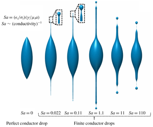
Figure 8. Effect of  $Sa$ on the drop shapes formed before breakup in the FC drop case (for
  $S=30$ and
  $\unicode[STIX]{x1D706}=30$). (a) Size of the progeny, (b) length of the jet, (c) the ratio of charge carried by the progeny droplet to its Rayleigh limit and (d) deformed drop shapes as a function of
  $Sa$ at the onset of progeny detachment.
3.2 Effect of conductivity
Figure 8(a) shows the effect of conductivity in terms of  $Sa$ on the size of the progeny formed during the Rayleigh breakup. It is observed that a liquid drop of higher conductivity will form smaller progenies. This is in agreement with the previous numerical studies (Burton & Taborek Reference Burton and Taborek2011; Collins et al. Reference Collins, Sambath, Harris and Basaran2013) as well as with the recent experimental observations, which indicate that the charged drops with higher conductivities eject thinner jets and subsequently smaller progeny droplets (Singh et al. Reference Singh, Gawande, Mayya and Thaokar2019b). A naive scaling of a balance of the electric time scale
  $t_{e}$ and the hydrodynamic time scale
  $t_{hl}$ leads to
  $l/a\sim Sa$. On the other hand, if we consider that the jet is issued after the conical tips approach the singularity, we find that the radius of the jet (
 $r_{j}$) is equivalent to the reciprocal of the curvature (
 $1/\unicode[STIX]{x1D705}$) at the tip of the drop that scales as
  $(t_{o}-t)^{1/2}$ (refer to Gawande et al. Reference Gawande, Mayya and Thaokar2017). In dimensional terms, this suggests that the jet radius
  $r_{j}/a\sim [(\tilde{t}_{o}-\tilde{t})/(\unicode[STIX]{x1D707}_{i}a/\unicode[STIX]{x1D6FE})]^{1/2}$. Realizing that the charge loss occurs over the electric time scale
  $(\tilde{t}_{o}-\tilde{t})\sim t_{e}$, leads to
  $r_{j}/a\sim Sa^{1/2}$. Thus over the length scale
  $l$, the jet has a lower charge and thereby the surface tension forces become dominant in the jet region. This leads to jet breakup by the Rayleigh Plateau instability and forms the progeny droplets of size equivalent to the radius of the jet. This qualitatively explains the progeny droplet size
  $r_{d}\sim Sa^{1/2}$ as observed in the simulations. Interestingly, similar scaling for the jet diameter is reported in a steady cone–jet electrospray system for the case where viscous forces and polarization forces dominate over inertia (Ganan-Calvo Reference Ganan-Calvo2004). The jet diameter is reported to scale as
  $r_{j}\sim [\unicode[STIX]{x1D707}_{i}Q_{f}/(S-1)\unicode[STIX]{x1D6FE}]^{1/2}$, where
  $Q_{f}$ is the volumetric flow rate in the electrospray system. The natural flow rate in the present problem can be written as
  $Q_{f}\sim a^{3}/(\tilde{t}_{o}-\tilde{t})$, which reduces to the similar scaling as obtained from our simulations. This indicates that, in the absence of inertia as considered in this work, when the hydrodynamic time scale becomes comparable to the charge relaxation time scales and the progeny is about to pinch off, the effect of tangential electric stress becomes significant, which results in the observed scaling. It should be noted, however, that the normal stresses continue to be higher than the tangential stresses throughout the process.
The asymptotic results of high  $Sa$ are in agreement with the perfect dielectric calculations (not discussed here) which are independent of the conductivity of the droplet. Thus, the weak scaling of
  $r_{d}$ (
 ${\sim}Sa^{0.1}$) at higher
  $Sa$ can be attributed to strong dielectric effects. Similarly, the scalings for the dimensional charge carried by the progeny can be explained by the singular scaling of charge density at the incipience of a jet, which is given by
  $q_{d}\sim [(t_{o}-t)/(\unicode[STIX]{x1D707}_{i}a/\unicode[STIX]{x1D6FE})]^{-1/2}$ (Gawande et al. Reference Gawande, Mayya and Thaokar2017). Thus, the total charge on the progeny droplet,
  $Q_{d}\sim q_{d}{r_{d}}^{2}$ implies that
  $Q_{d}\sim Sa^{1/2}$ over the electric time scale
  $t_{e}$. This, when dimensionalized and presented in terms of the fraction of the Rayleigh charge (
 $Q_{c}$), results in
  $\tilde{Q}_{d}\sim Q_{c}Sa^{-1/4}$ (figure 8b). This indicates that the Rayleigh fission of a charged droplet with high conductivity will produce marginally stable progeny droplets. This result is in agreement with the results predicted by potential flow analysis (Burton & Taborek Reference Burton and Taborek2011). It is also observed that the jet length increases with the decrease in conductivity and reaches a maximum value for
  $Sa=1.1$ but reduces for higher
  $Sa$ values (figure 8c).
The jet length is governed by a balance of tangential electric stress and the viscous stresses,  $\unicode[STIX]{x1D707}(v_{t}/r_{j})=qE_{t}$, where
  $v_{t}$ is the jet velocity. Since the radius of the jet and the charge scale as
  $Sa^{1/2}$ and
  $Sa^{-1/2}$ respectively, as shown earlier, and using the numerically obtained scaling of tangential electric field
  $E_{t}$ scaling as
  $Sa^{-1/3}$, and the jet elongation time scaling of
  $Sa^{1/2}$, the jet velocity is seen to scale as
  $Sa^{-1/3}$, which leads to the jet length scaling of
  $Sa^{1/6}$. The 1/6 scaling is seen in the simulations as well. The drop shapes at the onset of breakup for various
  $Sa$ (figure 8d) show that the drops with higher conductivity form a distinct jet before a progeny detaches from the tip of the drop. However, at lower conductivities, the dominance of capillary stresses occurs much earlier than the formation of a sustained jet and the droplet breakup occurs via end-lobe pinching from the tip of the drop.
3.3 Effect of viscosity contrast

Figure 9. (a) Drop shapes at the onset of end pinch off for various values of viscosity ratio ( $\unicode[STIX]{x1D706}$) (inset shows the blown up tips of the drop) and (b) scaling of progeny size and jet length with respect to viscosity ratio. Parameters used are
  $S=30$,
  $Sa=0.55$.
Further, to demonstrate the effect of viscosity contrast between a finitely conducting charged drop and the surrounding medium, the simulations were carried out for various  $\unicode[STIX]{x1D706}$ values. Figure 9(a) shows the deformed drop at the onset of pinch off for various values of the viscosity ratio at
  $S=30$ and
  $Sa=0.55$. It is observed that, when the viscosity of the drop is equal to the viscosity of the surrounding medium (
 $\unicode[STIX]{x1D706}=1$), which is a hypothetical case, the droplet deforms and forms a small progeny at the tip of the drop with small protrusion. However, a long sustained cylindrical jet is not observed in this case. This establishes that the sufficient viscous stresses are essential to balance the tangential electric stresses for the formation of a jet. This also therefore confirms the previous results (Burton & Taborek Reference Burton and Taborek2011), which shows that the inviscid formalism for Rayleigh breakup of a charged drop cannot predict the jet formation, although the progeny formation is observed due to charge convection effects. From figure 9 it can be observed that the length of the jet as well as the size of the progeny follow a 1/6 scaling with
  $\unicode[STIX]{x1D706}$. It is observed that, for a higher value of the viscosity ratio (
 $\unicode[STIX]{x1D706}\geqslant 150$), the thickness of the jet formed is less at the cone–jet transition region, which goes on increasing towards a thin thread connecting the progeny with the jet (as shown in the figure 9a inset). Thus, we propose that, for higher viscosity contrast between the drop and the surrounding medium, the drop will undergo breakup by ejecting one progeny (from each pole of the drop) followed by jet detachment.
4 Concluding remarks
This work investigates the formation of jet and progeny droplets due to a highly nonlinear breakup of a viscous drop charged to its Rayleigh limit. It is observed that the tangential electric stresses are important for the prediction of jet formation and the conductivity of the liquid drop determines the size and charge on the progeny droplets at the onset of their formation. It is also observed that the viscosity contrast between the drop and the surrounding medium is essential for the formation of long sustained jets and the drops with higher viscosity ratio can undergo breakup by jet detachment. The analysis presented in this work is valid when  $Oh\gg 1$. For example, the results presented in this work will hold for the case of 4 μm droplets for 1-octanol, 6 μm droplet for n-decanol or 32 μm droplet for 3-ethylene glycol. It is proposed that, since the droplets in processes such as electrospray or ionization in ion-mass spectroscopy eventually undergo Rayleigh fission at the smallest length scales, the viscous analysis does become relevant in these processes at late stages, and could actually explain the nanometre sized progeny droplets formed in the experiments on electrospray (Chen, Pui & Kaufman Reference Chen, Pui and Kaufman1995; Singh et al. Reference Singh, Khan, Koli, Sapra and Mayya2016). Thus, while the analysis reported by Collins et al. (Reference Collins, Jones, Harris and Basaran2008) and Gañán-Calvo et al. (Reference Gañán-Calvo, López-Herrera, Rebollo-Muñoz and Montanero2016) will hold good for prediction of the size of the first ejected droplet from the Taylor cone under an applied electric field, the final size distribution could be governed by the viscous scaling suggested in this work.

Figure 10. (a) Effect of nodes on the total surface charge without renormalization. The change in the total charge ( $\unicode[STIX]{x1D6FF}Q$) with time is indicated as a percentage of the initial charge (
 $Q=8.1\unicode[STIX]{x03C0}$). (b) Effect of nodes on the shape of the drop near breakup to check the convergence of the results with mesh refinement. (Parameters used are
  $S=30$,
  $Sa=15$,
  $\unicode[STIX]{x1D706}=30$.)
Declaration of interests
The authors report no conflict of interest.
Appendix
Conservation of total surface charge is critical in numerical analysis of the Rayleigh breakup of a charged drop problem. We therefore performed simulations with the same physical parameters but with different space discretizations to ascertain numerical convergence. The total charge on the drop is calculated after every iteration by integrating local surface charge density over the drop surface area. The total charge on the drop surface as a function of time during a typical Rayleigh breakup process is presented in figure 10(a). It is observed that, when the surface charge was allowed to change with time, the change in the total charge was less than 1 %. This result confirms that the implementation of an upwind scheme for solving the charge dynamics equation is correct and accurate to a precision of  $O(10^{-1})\,\%$. To avoid any charge loss due to numerical diffusion, we renormalized the charge by the initial charge on the drop. The renormalization is carried out particularly if the total charge value changes by 1 % of the initial charge.
Since the progeny droplets formed in the process are orders of magnitude smaller than the mother drop, the length scales change drastically. To capture the smallest length scales it is required to have higher resolution in the region where progenies are formed. Thus we used a non-uniform distribution of elements, where internode spacing increases in geometric progression from the north pole to the equator and decreases from the equator to the south pole. This ensures a higher number of elements (smaller grid size) near the poles as compared to the equatorial region. As the drop is assumed to be axisymmetric the grid size ( $\unicode[STIX]{x0394}s_{min}$) is always kept smaller than the minimum neck radius (
 $r_{min}$). The drop surface is populated with a higher number of node points when
  $r_{min}\leqslant \unicode[STIX]{x0394}s_{min}$. The charge density and the
  $r$–
$r$– $z$ coordinates of these nodes are obtained by cubic spline interpolation with respect to arclength. For convergence, tests of the simulations were carried out for four cases where the initial number of elements used were
  $N=50$, 100, 150, 200 and the drop shapes obtained are plotted in figure 10(b).
The numerical results are obtained for the entire drop and the perfect up–down symmetry obtained in our calculations was considered as the signature of correct implementation of the numerical scheme. Since the drop exhibits a perfect up–down symmetry across the equatorial plane, the upper half of the drop is presented here. The results showed that the size of the progeny converges for  $N=200$ and
  $N=250$ (as shown in figure 10b). Thus we used
  $N=200$ in all our further simulations.


