


1 Introduction
The nature of wall-bounded turbulent flows over rough surfaces, whose roughness distribution is homogeneous, has been studied extensively and is relatively well defined. To study such surfaces, engineers are equipped with tools such as the Moody chart (Moody Reference Moody1944) and the Hama roughness function (Hama Reference Hama1954). Most surfaces in nature and engineering applications, however, are heterogeneous and the heterogeneity can be arranged in an infinite number of ways. Examples include: rivets on aircraft, biofouling on ships, sedimentation on riverbeds and forest and crop boundaries in the atmospheric surface layer.
In this study, we consider a specific case of heterogeneous roughness where the roughness varies in the spanwise direction. Spanwise heterogeneity is imposed by alternating rough and smooth strips to form a test surface over which a turbulent boundary layer is developed. We investigate the behaviour of secondary flows as a function of the spanwise wavelength of heterogeneity with focus on the temporal as well as the time-average behaviour of these features.
1.1 Classification of spanwise heterogeneous roughness
Hinze (Reference Hinze1967) and later Anderson et al. (Reference Anderson, Barros, Christensen and Awasthi2015) showed that the secondary flows over spanwise heterogeneous rough surfaces are driven by the spanwise variation of Reynolds shear stress components and thus are Prandtl’s secondary flows of the second kind (Prandtl Reference Prandtl1952). Colombini & Parker (Reference Colombini and Parker1995) and Hwang & Lee (Reference Hwang and Lee2018) recognised two types of surfaces that induce spanwise variation of Reynolds shear stress: strip type (figure 1a), where spanwise variation of the Reynolds shear stress is affected by roughness variations or directly imposed, and ridge type (figure 1b), where spanwise variation of the Reynolds shear stress is affected by variations in surface elevation.

Figure 1. Types of spanwise heterogeneous roughness: (a) strip type and (b) ridge type (Colombini & Parker Reference Colombini and Parker1995; Hwang & Lee Reference Hwang and Lee2018). (a) White is the smooth strip, corresponding to low wall shear stress ( $\unicode[STIX]{x1D70F}_{s}$), black is the rough strip, corresponding to high wall shear stress (
 $\unicode[STIX]{x1D70F}_{r}$);
  $S$ is the width of the strips. (b)
  $L$ is the spacing between protruding elements,
  $b$ is the width of the elements,
  $h$ is the height of the elements and
  $\unicode[STIX]{x1D6FF}$ is the boundary-layer thickness (might be channel half-height or flow depth).
In numerical simulations, strip roughness can be modelled as spanwise alternating regions of high and low wall shear stress ( $\unicode[STIX]{x1D70F}_{r}$ and
  $\unicode[STIX]{x1D70F}_{s}$ in figure 1a) imposed directly as boundary conditions (Willingham et al. Reference Willingham, Anderson, Christensen and Barros2014; Chung, Monty & Hutchins Reference Chung, Monty and Hutchins2018). Superhydrophobic surfaces, with spanwise-alternating no-slip and free-slip boundary conditions can also be considered as such (Jelly, Jung & Zaki Reference Jelly, Jung and Zaki2014; Türk et al. Reference Türk, Daschiel, Stroh, Hasegawa and Frohnapfel2014; Lee, Jelly & Zaki Reference Lee, Jelly and Zaki2015; Stroh et al. Reference Stroh, Hasegawa, Kriegseis and Frohnapfel2016). Experimentally, surfaces can be constructed from spanwise alternating roughness strips (Hinze Reference Hinze1973; McLean Reference McLean1981; Nakagawa, Nezu & Tominaga Reference Nakagawa, Nezu and Tominaga1981; McLelland et al. Reference McLelland, Ashworth, Best and Livesey1999; Wang & Cheng Reference Wang and Cheng2005, Reference Wang and Cheng2006; Vermaas, Uijttewaal & Hoitink Reference Vermaas, Uijttewaal and Hoitink2011; Bai, Kevin & Monty Reference Bai, Hutchins and Monty2018).
The recessed part of previously investigated ridge-type roughness is typically a flat surface, while the elevated part has many possible cross-sectional shapes: rectangular (Wang & Cheng Reference Wang and Cheng2006; Hwang & Lee Reference Hwang and Lee2018; Medjnoun, Vanderwel & Ganapathisubramani Reference Medjnoun, Vanderwel and Ganapathisubramani2018, Reference Medjnoun, Vanderwel and Ganapathisubramani2020), trapezoidal (Nezu & Nakagawa Reference Nezu and Nakagawa1984), triangular (Goldstein & Tuan Reference Goldstein and Tuan1998; Medjnoun et al. Reference Medjnoun, Vanderwel and Ganapathisubramani2020; Zampiron, Cameron & Nikora Reference Zampiron, Cameron and Nikora2020), semicircle (Medjnoun et al. Reference Medjnoun, Vanderwel and Ganapathisubramani2020), streamwise-aligned pyramids (Yang & Anderson Reference Yang and Anderson2018) and smoother, sinusoidal-like spanwise elevation variations (Colombini Reference Colombini1993; Wang & Cheng Reference Wang and Cheng2006; Awasthi & Anderson Reference Awasthi and Anderson2018). Studied surfaces often involve a combination of both ridge-type and strip-type roughnesses (Vanderwel & Ganapathisubramani Reference Vanderwel and Ganapathisubramani2015; Vanderwel et al. Reference Vanderwel, Stroh, Kriegseis, Frohnapfel and Ganapathisubramani2019; Stroh et al. Reference Stroh, Schäfer, Frohnapfel and Forooghi2020). Surfaces with multiple spanwise roughness wavelengths (Barros & Christensen Reference Barros and Christensen2014) have also been studied.
A slightly different class of spanwise heterogeneity has been studied by Kevin et al. (Reference Monty, Bai, Pathikonda, Nugroho, Barros, Christensen and Hutchins2017) based on alternating arrangements of directional/anisotropic rough surfaces. However, both strip-type and ridge-type roughnesses in figure 1(a,b) have isotropic local roughness, whereas converging–diverging (C–D) riblets (Nugroho, Hutchins & Monty Reference Nugroho, Hutchins and Monty2013; Kevin et al. Reference Monty, Bai, Pathikonda, Nugroho, Barros, Christensen and Hutchins2017; Kevin & Hutchins Reference Monty and Hutchins2019b) have spanwise varying anisotropy or directionality. Converging–diverging riblets also generate secondary flows even in laminar boundary layers (Xu, Zhong & Zhang Reference Xu, Zhong and Zhang2018), where no spanwise gradients of Reynolds shear stress are present. This possibly suggests a different generation mechanism to Prandtl’s secondary flows (of the second kind) typically attributed to spanwise heterogeneous roughness.
1.2 The effect of spanwise heterogeneity on turbulent boundary layers
The effect of spanwise heterogeneity-induced secondary flows is observed as thickening and thinning of boundary-layer thickness in the cross-plane of the boundary layer (Nugroho et al. Reference Nugroho, Hutchins and Monty2013; Barros & Christensen Reference Barros and Christensen2014; Vanderwel & Ganapathisubramani Reference Vanderwel and Ganapathisubramani2015; Kevin et al. Reference Monty, Bai, Pathikonda, Nugroho, Barros, Christensen and Hutchins2017; Medjnoun et al. Reference Medjnoun, Vanderwel and Ganapathisubramani2018). This is associated with the formation of high momentum (HMPs) and low momentum pathways (LMPs) above the surfaces (Barros & Christensen Reference Barros and Christensen2014; Willingham et al. Reference Willingham, Anderson, Christensen and Barros2014; Anderson et al. Reference Anderson, Barros, Christensen and Awasthi2015).
Hinze (Reference Hinze1967) hypothesised the occurrence of secondary flows as a consequence of the production–dissipation imbalance of turbulent kinetic energy over spanwise heterogeneity. For strip-type roughness (figure 1a), production exceeds the dissipation above the  $\unicode[STIX]{x1D70F}_{r}$ strips, transferring turbulent-rich flow to the adjacent
  $\unicode[STIX]{x1D70F}_{s}$ strips, and vice versa. This results in a secondary flow above the roughness interface between
  $\unicode[STIX]{x1D70F}_{r}$ and
  $\unicode[STIX]{x1D70F}_{s}$, with upwelling above
  $\unicode[STIX]{x1D70F}_{s}$ strips and downwelling above
  $\unicode[STIX]{x1D70F}_{r}$. Locally, due to lift-up, there will be low momentum pathways associated with upwelling, and high momentum pathways associated with downwelling. In ridge-type roughness, the secondary flow occurs somewhere near the junction between the raised and recessed sections of the surface, with the upwelling either above the junction (Wang & Cheng Reference Wang and Cheng2006) or above the ridge (Nezu & Nakagawa Reference Nezu and Nakagawa1984; Colombini Reference Colombini1993; Medjnoun et al. Reference Medjnoun, Vanderwel and Ganapathisubramani2018).
Recent studies showed that the size, spanwise location and direction of the secondary flows may be affected by the specific configuration of spanwise heterogeneity (Goldstein & Tuan Reference Goldstein and Tuan1998; Wang & Cheng Reference Wang and Cheng2006; Türk et al. Reference Türk, Daschiel, Stroh, Hasegawa and Frohnapfel2014; Vanderwel & Ganapathisubramani Reference Vanderwel and Ganapathisubramani2015; Stroh et al. Reference Stroh, Hasegawa, Kriegseis and Frohnapfel2016; Awasthi & Anderson Reference Awasthi and Anderson2018; Chung et al. Reference Chung, Monty and Hutchins2018; Hwang & Lee Reference Hwang and Lee2018; Medjnoun et al. Reference Medjnoun, Vanderwel and Ganapathisubramani2018; Yang & Anderson Reference Yang and Anderson2018; Medjnoun et al. Reference Medjnoun, Vanderwel and Ganapathisubramani2020; Zampiron et al. Reference Zampiron, Cameron and Nikora2020). For strip-type roughness, the spanwise roughness wavelength  $\unicode[STIX]{x1D6EC}=2S$ (figure 1a) seems to determine the behaviour of the secondary flows. The effect of the roughness half-wavelength
  $S$ is shown by Chung et al. (Reference Chung, Monty and Hutchins2018), where the flow, far removed from the secondary flows, speeds up above the smooth strips and slows down above the rough strips when
  $S\gg \unicode[STIX]{x1D6FF}$ (figure 2a), which is as would be expected for flow over homogeneous roughness. The opposite occurs when
  $S\approx \unicode[STIX]{x1D6FF}$ (figure 2b), where the secondary flows are space filling. When
  $S\ll \unicode[STIX]{x1D6FF}$ (figure 2c), the size of the secondary flows decreases and the flow approaches spanwise homogeneity for
  $z\gtrsim S$. The effect of spanwise roughness wavelength in superhydrophobic surfaces is also explored in Türk et al. (Reference Türk, Daschiel, Stroh, Hasegawa and Frohnapfel2014) and Stroh et al. (Reference Stroh, Hasegawa, Kriegseis and Frohnapfel2016). For ridge-type roughness, the contributing factors are shown in figure 1(b): the spacing between ridges
  $L$ (Goldstein & Tuan Reference Goldstein and Tuan1998; Vanderwel & Ganapathisubramani Reference Vanderwel and Ganapathisubramani2015; Medjnoun et al. Reference Medjnoun, Vanderwel and Ganapathisubramani2018; Yang & Anderson Reference Yang and Anderson2018; Zampiron et al. Reference Zampiron, Cameron and Nikora2020), the width
  $b$ (Hwang & Lee Reference Hwang and Lee2018; Medjnoun et al. Reference Medjnoun, Vanderwel and Ganapathisubramani2020) and height
  $h$ of the ridge (Wang & Cheng Reference Wang and Cheng2006; Awasthi & Anderson Reference Awasthi and Anderson2018; Yang & Anderson Reference Yang and Anderson2018). As the geometry of the spanwise roughness becomes more complicated (Vanderwel & Ganapathisubramani Reference Vanderwel and Ganapathisubramani2015), the resulting secondary flows are a combination of the aforementioned factors.

Figure 2. Illustration of surfaces with spanwise heterogeneous roughness, similar to that shown in Chung et al. (Reference Chung, Monty and Hutchins2018): (a) limiting case  $S/\unicode[STIX]{x1D6FF}\gg 1$, (b) intermediate case
  $S/\unicode[STIX]{x1D6FF}\approx 1$ and (c) limiting case
  $S/\unicode[STIX]{x1D6FF}\ll 1$. The boundary-layer thickness is - - -; areas bounded by
  $\cdots \cdots$ show regions approaching spanwise homogeneity.
In the existing studies, these secondary flows are almost always discussed in the time-averaged sense. Recent studies, however, have uncovered certain time-dependent features of the secondary flows which are masked by time averaging. A hint of these features is given by the one-dimensional (1-D) energy spectrograms (Nugroho et al. Reference Nugroho, Hutchins and Monty2013; Awasthi & Anderson Reference Awasthi and Anderson2018; Medjnoun et al. Reference Medjnoun, Vanderwel and Ganapathisubramani2018; Zampiron et al. Reference Zampiron, Cameron and Nikora2020), two-point correlation maps (Kevin et al. Reference Monty, Bai, Pathikonda, Nugroho, Barros, Christensen and Hutchins2017; Kevin & Hutchins Reference Monty and Hutchins2019b) and proper orthogonal decomposition of the turbulent fluctuation fields (Vanderwel et al. Reference Vanderwel, Stroh, Kriegseis, Frohnapfel and Ganapathisubramani2019). A streamwise periodic behaviour is implicit in many of these results, reminiscent of the meandering of very large-scale motions (VLSM) that occur naturally in the log layer of wall-bounded turbulence (Hutchins & Marusic Reference Hutchins and Marusic2007a). Meandering of the secondary flows induced by spanwise heterogeneity, akin to that observed for VLSMs, has been shown in Kevin et al. (Reference Monty, Bai, Pathikonda, Nugroho, Barros, Christensen and Hutchins2017), Kevin & Hutchins (Reference Monty and Hutchins2019b) and Vanderwel et al. (Reference Vanderwel, Stroh, Kriegseis, Frohnapfel and Ganapathisubramani2019) for a surface whose spanwise wavelength is approximately equal to  $\unicode[STIX]{x1D6FF}$ (close to the expected spanwise scale of the VLSM). These findings pose a further question about the meandering behaviour where the roughness wavelength is not equal to
  $\unicode[STIX]{x1D6FF}$. A recent study in ridge-type roughness by Zampiron et al. (Reference Zampiron, Cameron and Nikora2020) showed the possibility of coexistence between the meandering secondary flows and VLSM when the roughness spacing is approximately
  $4\unicode[STIX]{x1D6FF}$. However, it should be noted that the behaviour of the secondary flows in ridge-type roughness is deeply affected by the geometry and size of the ridges. Furthermore, it has been shown in Stroh et al. (Reference Stroh, Schäfer, Frohnapfel and Forooghi2020) that increasing spanwise variation in virtual origin can reverse the direction of secondary flows.
In this study, we aim to isolate a pure strip-type roughness, similar to that of Hinze (Reference Hinze1967, Reference Hinze1973), by minimising variations in surface elevation between roughness strips. In the absence of ridge-related behaviour, we explore the effects of spanwise roughness wavelength  $2S$ on the resulting secondary flows over a range of
  $S/\overline{\unicode[STIX]{x1D6FF}}$ (
 $0.32\leqslant S/\overline{\unicode[STIX]{x1D6FF}}\leqslant 6.81$). This range is chosen to represent the intermediate cases,
  $S/\unicode[STIX]{x1D6FF}\approx 1$, where meandering secondary flows have been observed (Kevin et al. Reference Monty, Bai, Pathikonda, Nugroho, Barros, Christensen and Hutchins2017; Kevin & Hutchins Reference Monty and Hutchins2019b; Vanderwel et al. Reference Vanderwel, Stroh, Kriegseis, Frohnapfel and Ganapathisubramani2019), and the two limits where
  $S/\unicode[STIX]{x1D6FF}\gg 1$ and
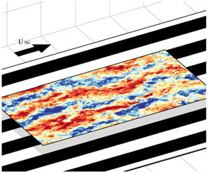
  $S/\unicode[STIX]{x1D6FF}\ll 1$. To further study the time-dependent behaviour of the secondary flows, we focus on the fluctuating as well as the time-averaged velocity components. We conduct hot-wire anemometry (HWA) and particle image velocimetry (PIV) measurements on turbulent boundary layers developing over surfaces composed of streamwise-aligned strips of sandpaper separated by smooth strips of cardboard laid down in a spanwise-alternating pattern. PIV measurements capture the flow field in two planes: stereoscopic PIV (SPIV) in the spanwise–wall-normal plane and wall-parallel PIV (WPPIV) in the streamwise–spanwise plane (figure 7b).

Figure 3. Triple decomposition of streamwise velocity  $u$ for case SR50 (
 $S/\overline{\unicode[STIX]{x1D6FF}}=0.62$).
The instantaneous velocity components are defined as  $\boldsymbol{u}=(u,v,w)$, corresponding to the axis system
  $\boldsymbol{x}=(x,y,z)$. Here,
  $x$,
$x$,  $y$ and
  $z$ refer to the streamwise, spanwise and wall-normal directions, respectively. Due to spanwise periodicity,
  $\boldsymbol{u}$ can be decomposed into its temporal and spatial average, similar to the decomposition method utilised in Raupach & Shaw (Reference Raupach and Shaw1982), Finnigan (Reference Finnigan2000) and Coceal et al. (Reference Coceal, Thomas, Castro and Belcher2006). The total velocity
  $\boldsymbol{u}$ at a particular
  $x$ location can be triply decomposed into
 $$\begin{eqnarray}\displaystyle \boldsymbol{u}(y,z,t) & = & \displaystyle \boldsymbol{U}(y,z)+\boldsymbol{u}^{\prime }(y,z,t)\end{eqnarray}$$
 $$\begin{eqnarray}\displaystyle & = & \displaystyle \langle \boldsymbol{U}\rangle _{\unicode[STIX]{x1D6EC}}(z)+\widetilde{\boldsymbol{U}}(y,z)+\boldsymbol{u}^{\prime }(y,z,t)\end{eqnarray}$$
 $$\begin{eqnarray}\displaystyle & = & \displaystyle \langle \boldsymbol{U}\rangle _{\unicode[STIX]{x1D6EC}}(z)+\widetilde{\boldsymbol{u}}^{\prime }(y,z,t),\end{eqnarray}$$
 where  $\boldsymbol{U}$ is the Reynolds (temporal) average, or the local mean velocity, and
  $\boldsymbol{u}^{\prime }$ is the turbulent fluctuation;
  $\boldsymbol{U}$ can be further decomposed into its
  $yt$ average
  $\langle \boldsymbol{U}\rangle _{\unicode[STIX]{x1D6EC}}$, or the global mean over the span, and the time-averaged spatial variations about this mean
  $\widetilde{\boldsymbol{U}}$. We also introduce the quantity
  $\widetilde{\boldsymbol{u}}^{\prime }$, which is the combination of
  $\widetilde{\boldsymbol{U}}$ and
  $\boldsymbol{u}^{\prime }$. An example of this triple decomposition for the streamwise velocity
  $u$ is shown in figure 3. Here,
  $\widetilde{U}$ shows the presence of low-speed flows above the smooth strips and high-speed flows above the rough strips, which coincide with the common flow up and down of the mean secondary flows, respectively (figure 8e). The asymmetry of
  $\widetilde{U}$ in figure 3 is due to the lack of convergence in the rough-wall SPIV data, where we only have 4800 realisations at each
  $(y,z)$ position for computing
  $\widetilde{U}$.
2 Experimental set-up
2.1 Facility
The measurements are performed in an open return boundary-layer wind tunnel in the Walter Basset Aerodynamics Laboratory at the University of Melbourne. A complete description of this facility is given in Harun et al. (Reference Harun, Monty, Mathis and Marusic2013). The test section has the dimensions of  $6.7~\text{m}\times 0.94~\text{m}\times 0.38~\text{m}$ (length
  $\times$ width
  $\times$ height), with measurements made in the turbulent boundary layer developing over the lower surface. The free-stream turbulence level is
  ${\approx}0.3\,\%$. The boundary layer is tripped by a strip of P-40 sandpaper (length 115 mm) at the beginning of the test section.
The streamwise pressure coefficient  $C_{p}\equiv 2\unicode[STIX]{x0394}P/\unicode[STIX]{x1D70C}U_{\infty }^{2}$ is measured for each surface in this study using 11 static pressure taps located at the roof of the tunnel, spaced approximately by 0.5 m in
  $x$, from
  $x=0$ to 5.5 m (
 $x=0$ is at the end of the trip, at the inlet of the working section);
  $\unicode[STIX]{x0394}P$ is the difference between the static pressure measured on each tap and the reference tap above the trip,
  $\unicode[STIX]{x1D70C}$ is the density of air and
  $U_{\infty }$ is the free-stream velocity. For all heterogeneous surfaces, the magnitude of
  $C_{p}$ varies within
  $\pm 0.013$ along the length of the test section. This range is very close to the
  $C_{p}$ variation (
 $C_{p}\pm 0.01$) observed for the zero-pressure-gradient smooth-wall cases conducted in the same facility previously by Harun et al. (Reference Harun, Monty, Mathis and Marusic2013).
2.2 Spanwise heterogeneous cases
Spanwise heterogeneous surfaces are constructed from strips of P-36 grit sandpaper (rough patch) and 2 mm thick cardboard (smooth patch) of equal width  $S$, as shown in figure 4(b). These strips are assembled in a spanwise-alternating pattern, covering the first 5.6 m of the test section after the trip (from
  $x=0$ and extending to
  $x=5.6~\text{m}$), such that the surfaces have periodic rough and smooth patches of wavelength
  $\unicode[STIX]{x1D6EC}=2S$. The use of the 2 mm thick cardboard strips for the smooth patches ensures, as far as possible, that the heterogeneity is imposed by the spanwise shear stress variation between the cardboard and sandpaper strips rather than any mismatch in virtual origin (strip- rather than ridge-type heterogeneity, figure 1). The thickness of the cardboard is selected to minimise variation in the virtual origin between the rough and smooth strips. A laser scan of a
  $60~\text{mm}\times 20~\text{mm}$ sample of this surface (figure 4a) reveals that the cardboard surface is close to the maximum height of the sand grains, with the average height of the sandpaper grain 0.728 mm lower than the cardboard, and the maximum peak height of the sandpaper approximately 0.324 mm above the cardboard. The mean grain size of the sandpaper roughness is
  $k=0.902~\text{mm}$ with
  $k_{s}=1.96~\text{mm}$ (Squire et al. Reference Squire, Morrill-Winter, Hutchins, Schultz, Klewicki and Marusic2016), which corresponds to
  $\unicode[STIX]{x1D6FF}_{s}/k\approx 63$ for the wind tunnel conditions used here (where
  $\unicode[STIX]{x1D6FF}_{s}$ is the smooth wall boundary layer at
  $x=4~\text{m}$ and
  $k$ is the mean grain size of the sandpaper strip). For the spanwise heterogeneous surfaces, the equivalent sand grain roughness
  $k_{s}$ and the true virtual origin are unknown and, in fact, not well defined.

Figure 4. (a) Magnified view of  $20~\text{mm}\times 20~~\text{mm}$ sample of the spanwise heterogeneous surface. Rough patch profile is obtained from a laser profilometer. (b) Spanwise heterogenous surface and measurement plane at 4 m downstream of the inlet to the working section. The white and black patches correspond to strips of cardboard and sandpaper, respectively. (c) Hot-wire anemometry measurement grid. Measurements start at the centre of a smooth patch (——, blue) and end at the centre of the adjacent rough patch (——, red).
  $S$ is the width of the roughness strips.
Table 1. Summary of spanwise heterogeneous roughness cases and the reference smooth- and rough-wall cases. The statistics are obtained from HWA:  $\overline{\unicode[STIX]{x1D6FF}}$ is the spanwise-averaged 98 % boundary-layer thickness of the surface with spanwise heterogeneity, while
  $\unicode[STIX]{x1D6FF}_{s}$ and
  $\unicode[STIX]{x1D6FF}_{r}$ are the 98 % boundary-layer thickness of the reference smooth- and rough-wall cases, respectively;
  $\overline{\unicode[STIX]{x1D703}}$ is the spanwise-averaged momentum thickness of the spanwise heterogeneous surfaces, while
  $\unicode[STIX]{x1D703}_{s}$ and
  $\unicode[STIX]{x1D703}_{r}$ are the momentum thickness of the reference smooth- and rough-wall cases, respectively. Reynolds number definitions are:
  $Re_{x}\equiv xU_{\infty }/\unicode[STIX]{x1D708}$,
  $Re_{\unicode[STIX]{x1D6FF}}\equiv \unicode[STIX]{x1D6FF}U_{\infty }/\unicode[STIX]{x1D708}$, and
  $Re_{\unicode[STIX]{x1D703}}\equiv \unicode[STIX]{x1D703}U_{\infty }/\unicode[STIX]{x1D708}$. The last three columns show the availability of data from all measurement methods: HWA, SPIV and WPPIV.

Table 1 describes all spanwise heterogeneous roughness (‘SR’) cases in this study. Five surfaces with varying  $S$ are constructed for this study to achieve a range of
  $S/\overline{\unicode[STIX]{x1D6FF}}=0.32{-}6.81$. Here,
  $S$ is normalised by the spanwise-averaged boundary-layer thickness
  $\overline{\unicode[STIX]{x1D6FF}}$. The variation of boundary-layer thickness
  $\unicode[STIX]{x1D6FF}(y)$ across the span is under
  $\pm 20\,\%$ of its mean.
All SR cases, except for SR250-1, are carried out at matched free-stream velocity  $U_{\infty }\approx 15~\text{m}~\text{s}^{-1}$ at
  $x=4~\text{m}$. Due to the limited test section width (0.94 m), measurements are carried out at
  $x=1.85~\text{m}$ for SR250-1 to achieve
  $S/\overline{\unicode[STIX]{x1D6FF}}=6.81$.
2.3 Reference cases
Two reference cases for spanwise homogeneous conditions are included in table 1 for comparison to SR cases. The first is the reference smooth-wall case (‘SW’) and the second is the reference rough-wall case (‘RW’), where the surface is constructed entirely from a sheet of P-36 grit sandpaper (the same sandpaper used to form the roughness strips for the SR cases). HWA measurements for these reference cases are taken at similar  $Re_{x}\equiv xU_{\infty }/\unicode[STIX]{x1D708}$ to their spanwise heterogeneous counterparts, that is, SW-1 and RW-1 for case SR250-1 at
  $x=1.85~\text{m}$, SW-2 and RW-2 for all other cases at
  $x=4~\text{m}$.
Table 2. Summary of reference smooth- and rough-wall cases in viscous-scaled units.  $\unicode[STIX]{x1D6FF}_{s}$ and
  $\unicode[STIX]{x1D6FF}_{r}$ are the 98 % boundary-layer thickness for the smooth- and rough-wall reference cases, respectively, and
  $\unicode[STIX]{x1D6FF}_{s}^{+}\equiv \unicode[STIX]{x1D6FF}_{s}U_{\unicode[STIX]{x1D70F}}/\unicode[STIX]{x1D708}$,
  $\unicode[STIX]{x1D6FF}_{r}^{+}\equiv \unicode[STIX]{x1D6FF}_{r}U_{\unicode[STIX]{x1D70F}}/\unicode[STIX]{x1D708}$.
  $l^{+}$ is the viscous-scaled length of the etched portion of the hot-wire. Coefficient of friction is defined as
  $C_{f}\equiv 2(U_{\unicode[STIX]{x1D70F}}/U_{\infty })^{2}$.


Figure 5. Boundary-layer profiles from hot-wire measurements of reference smooth- and rough-wall cases, SW-1, SW-2, RW-1 and RW-2 (legend in table 2). (a) Mean streamwise velocity profile  $U^{+}$; - - -,
  $(1/0.384)\log z^{+}+4.17$. (b) Turbulence intensity
  $\overline{u^{\prime }u^{\prime }}^{+}$; DNS (Sillero, Jiménez & Moser Reference Sillero, Jiménez and Moser2014), filtered according to the spatial resolution
  $l^{+}$ for SW-1 (——, grey) and SW-2 (——, black). (c) Velocity defect profile
  $U_{\infty }^{+}-U^{+}$; - - -,
 $2.3-(1/0.384)\log (z/\unicode[STIX]{x1D6FF}_{99})$, where
  $\unicode[STIX]{x1D6FF}_{99}$ is the 99 % boundary-layer thickness. Data points are downsampled for clarity.
For the SW cases, the wall friction velocity  $U_{\unicode[STIX]{x1D70F}}$ is determined by fitting the mean velocity profile from HWA measurements to the composite profile of Chauhan, Monkewitz & Nagib (Reference Chauhan, Monkewitz and Nagib2009). In the outer region, the smooth-wall turbulent boundary-layer profile follows
 $$\begin{eqnarray}U^{+}=\frac{1}{\unicode[STIX]{x1D705}}\log z^{+}+A+\frac{2\unicode[STIX]{x1D6F1}}{\unicode[STIX]{x1D705}}{\mathcal{W}}\left(\frac{z}{\unicode[STIX]{x1D6FF}}\right),\end{eqnarray}$$
 where subscript ‘ $+$’ denotes viscous scaling of velocity and length
  $U^{+}\equiv U/U_{\unicode[STIX]{x1D70F}}$,
  $z^{+}\equiv zU_{\unicode[STIX]{x1D70F}}/\unicode[STIX]{x1D708}$, where
  $\unicode[STIX]{x1D705}$ is the von Kármán constant,
  $\unicode[STIX]{x1D6F1}$ is the wake parameter and
  ${\mathcal{W}}$ is the modified wake function (Chauhan et al. Reference Chauhan, Monkewitz and Nagib2009). Here,
  $\unicode[STIX]{x1D705}=0.384$ and
  $A=4.17$, following Marusic et al. (Reference Marusic, Chauhan, Kulandaivelu and Hutchins2015). The viscous-scaled parameters for the reference cases are summarised in table 2.
For the RW cases, the profile is shifted from (2.1) according to the Hama roughness function (Hama Reference Hama1954),
 $$\begin{eqnarray}\unicode[STIX]{x0394}U^{+}=\frac{1}{\unicode[STIX]{x1D705}}\log k_{s}^{+}+A-A_{FR},\end{eqnarray}$$
 where  $k_{s}^{+}\equiv k_{s}U_{\unicode[STIX]{x1D70F}}/\unicode[STIX]{x1D708}$ and
  $A_{FR}$ is 8.5, following Nikuradse (Reference Nikuradse1933). As shown in table 2,
  $k_{s}\approx 2~\text{mm}$ for both RW-1 and RW-2, close to that obtained by Squire et al. (Reference Squire, Morrill-Winter, Hutchins, Schultz, Klewicki and Marusic2016) for the same P-36 sandpaper surface. This value translates to 98 and 91 viscous units for RW-1 and RW-2, respectively.
HWA-measured boundary-layer profiles for these reference cases are shown in figure 5. Figure 5(a) shows that  $U^{+}$ for the smooth-wall reference cases SW-1 and SW-2 collapses to the log law
  $\unicode[STIX]{x1D705}^{-1}\log z^{+}+A$, while
  $U^{+}$ for the rough-wall cases RW-1 and RW-2 is shifted by
  $\unicode[STIX]{x0394}U^{+}\approx 7.5$ from this line. Viscous-scaled turbulence intensities
  $\overline{u^{\prime }u^{\prime }}^{+}$ are shown in figure 5(b). Reasonable collapse is observed for SW-1 and SW-2 to the direct numerical simulation (DNS) results of Sillero et al. (Reference Sillero, Jiménez and Moser2014) at matched
  $Re_{\unicode[STIX]{x1D703}_{s}}\equiv \unicode[STIX]{x1D703}_{s}U_{\infty }/\unicode[STIX]{x1D708}$, where
  $\unicode[STIX]{x1D703}_{s}$ is the momentum thickness of the reference smooth-wall cases. It should be noted that the
  $\overline{u^{\prime }u^{\prime }}$ attributed to the DNS results have been modified to account for the expected attenuation due to the hot-wire spatial resolution
  $l^{+}\equiv lU_{\unicode[STIX]{x1D70F}}/\unicode[STIX]{x1D708}$ (table 2) utilised in this study. That is, the missing energy, which is assumed to be function of
  $l^{+}$, has been subtracted from the original DNS statistics, following the approach of Lee, Kevin & Hutchins (Reference Lee, Monty and Hutchins2016). A measure of outer-layer similarity for these reference cases is given in figure 5(c), where velocity defect profiles
  $U_{\infty }^{+}-U^{+}$ for all cases collapse to the line
  $2.3-\unicode[STIX]{x1D705}^{-1}\log (z/\unicode[STIX]{x1D6FF}_{99})$, consistent with Marusic et al. (Reference Marusic, Chauhan, Kulandaivelu and Hutchins2015).
2.4 Hot-wire anemometry
Two sets of hot-wire measurements of streamwise velocity are performed for each case of spanwise heterogeneity in table 1. The first is a wall-normal traverse at 40 logarithmically spaced  $z$ locations over the centre of the smooth patch to obtain the near-wall profile. The second is a measurement over a spanwise–wall-normal grid, in which profiles are obtained at 11 (cases SR25–SR160) and 15 (cases SR250-1 and SR250-2) spanwise locations over one half-wavelength
  $S$. The grid spans from the midpoint of the smooth patch to the midpoint of the adjacent rough patch (figure 4c). At each spanwise location, the boundary layer is traversed at 30 logarithmically spaced wall-normal locations. For both smooth- and rough-wall reference cases (SW and RW), only the wall-normal traverse is conducted at the spanwise centre of the test section.
Hot-wire measurements are carried out using a modified Dantec 55P05 single-sensor boundary-layer probe attached to a Dantec 55H21 probe support. The sensor is made by soldering a Woolaston wire with a  $5~\unicode[STIX]{x03BC}\text{m}$ diameter platinum core to the tip of the probe. A 1 mm long portion of the wire is etched with nitric acid solution to remove the silver coating, yielding the recommended wire length-to-diameter ratio of 200 (Ligrani & Bradshaw Reference Ligrani and Bradshaw1987). The viscous-scaled etched lengths
  $l^{+}$ for the reference cases are shown in table 2. The anemometer used in this study is an in-house constant-temperature anemometer (MUCTA) with a fixed overheat ratio of 1.8. The output signal from the constant-temperature anemometer (CTA) is sampled at 30 kHz and low-pass filtered at the cutoff frequency of 15 kHz, corresponding to
  $t^{+}\sim O(1)$. Sampling time
  $T$ is set to maintain turnover times
  $TU_{\infty }/\unicode[STIX]{x1D6FF}\geqslant 20\,000$ (Hutchins et al. Reference Hutchins, Nickels, Marusic and Chong2009), thus allowing the convergence of energy spectra.
The hot-wire probe is calibrated before and after each measurement to obtain the output voltage and streamwise velocity relationship, which is fitted with a third-order polynomial. For the wall-normal traverse, time-based interpolation is applied between pre- and post-calibration curves to compensate for a slight sensor drift. For the spanwise–wall-normal grid measurements, which take longer times, the hot-wire voltage in the free stream is monitored after each wall-normal traverse to account for sensor drift using a modified version of the methodology suggested by Talluru et al. (Reference Talluru, Kulandaivelu, Hutchins and Marusic2014).

Figure 6. (a) Field of view of stereoscopic PIV measurements, stitched from front camera (C $_{F}$) and rear camera (C
 $_{R}$). (b) Schematic of stereoscopic PIV set-up.

Figure 7. (a) Field of view of wall-parallel PIV measurements, stitched from 3 cameras: C $_{1}$, C
 $_{2}$ and C
 $_{3}$. (b) Schematic of wall-parallel PIV set-up.
  $z_{sheet}$ is the distance between the laser sheet and the wall.

Figure 8. Contours of mean streamwise velocity  $U/U_{\infty }$ for reference smooth-wall case SW-2 (a) and spanwise heterogeneous (SR) cases (b–g). All data are obtained from SPIV measurements except for (b), which data are obtained from HWA measurements. The white and black patches correspond to smooth and rough strips, respectively. Vectors indicate
  $V$ and
  $W$, downsampled for clarity. Solid white lines mark the three spanwise locations related to the mean secondary flows: common flow up (ⓤ), centre of a mean secondary flow (ⓒ) and common flow down (ⓓ). White dashed lines are the 98 % boundary-layer thickness
  $\unicode[STIX]{x1D6FF}$ as a function of
  $y$.
$y$.
2.5 Stereoscopic PIV
Non-time-resolved cross-stream plane ( $y$–
$y$– $z$) stereoscopic PIV experiments are performed at
  $x=4$ m. As shown in table 1, SPIV data are available for all spanwise heterogeneous cases and the reference smooth wall, except for cases located at
  $x=1.85~\text{m}$ (SR250-1 and SW-1) due to limited optical access. SPIV measurements are also not conducted on the reference rough-wall cases (RW-1 and RW-2).
The complete description of the experimental set-up and PIV parameters are given in appendix A. SPIV images are captured from two pco.4000 cameras positioned upstream and downstream of the  $y$–
$y$– $z$-plane (figure 6b). The current set-up gives a field of view (FOV) of approximately
  $4\unicode[STIX]{x1D6FF}_{s}\times 3\unicode[STIX]{x1D6FF}_{s}$ (figure 6a), where
  $\unicode[STIX]{x1D6FF}_{s}$ corresponds to the SW-2 case. The FOV width is 240 mm or
  ${\geqslant}2S$ for SR25, SR50, and SR100, but
  ${<}2S$ for case SR160 and SR250-2. For these two cases, the FOV is limited to the region near to the rough-to-smooth interface and a complete pair of roll modes is not captured. Furthermore, since a full wavelength is not captured for these two cases, the global mean
  $\langle \boldsymbol{U}\rangle _{\unicode[STIX]{x1D6EC}}$ and the time-averaged, spanwise variations
  $\widetilde{\boldsymbol{U}}$ in (1.2) are obtained by reflecting the FOV about the centre of a smooth strip (
 $y=0$).
2.6 Wall-parallel PIV
In order to more fully capture the spatio-temporal variation of the roll modes, PIV measurements are performed on streamwise–spanwise ( $x$–
$x$– $y$) planes, parallel to the surfaces and non-simultaneous with the SPIV measurements. As with the SPIV, WPPIV measurements are not conducted for cases located at 1.85 m downstream of the trip (SR250-1 and SW-1, table 1) or for the reference rough-wall cases (RW-1 and RW-2).
The complete description of the experimental set-up and PIV parameters are given in appendix B. The streamwise extent of the FOV (figure 7a) extends from  $x=3.5~\text{m}$ to
  $x=4.01~\text{m}$, covering approximately
  $9\unicode[STIX]{x1D6FF}_{s}$ in the streamwise direction, and is constructed by stitching together three pco.4000 cameras (figure 7b). The spanwise width of the FOV is 270 mm or
  ${\geqslant}2S$ for SR25, SR50 and SR100, but
  ${<}2S$ for case SR160 and SR250-2. Similar to the SPIV measurements, the FOV is limited to the region close to the rough-to-smooth interface for case SR160 and SR250-2 and a complete pair of roll modes is not captured for these cases. To capture the roll modes forming above the spanwise heterogeneous roughness surfaces, the WPPIV laser sheet is set at some distance
  $z_{sheet}$ from the wall (figure 7b), approximately at the centre of the mean secondary flows (figure 8). For the reference smooth-wall case SW-2, the laser sheet is set at
  $z_{sheet}/\unicode[STIX]{x1D6FF}_{s}=0.5$.
3 Mean velocity fields
3.1 Mean streamwise velocity
Figure 8 shows the contours of mean streamwise velocity profiles  $U$ for the reference smooth-wall case SW-2 (figure 8a) and all spanwise heterogeneous (SR) cases in table 1 (figure 8b–g). Contours are obtained from SPIV measurements, except for case SR250-1 (figure 8b) due to limited optical access at the streamwise location where the measurements are taken. For this case, the contours are constructed from the spanwise–wall-normal grid of HWA measurements. Since no attempt is made to measure
  $U_{\unicode[STIX]{x1D70F}}$ for these cases, we present
  $U$ normalised by the free-stream velocity
  $U_{\infty }$ as a function of outer-scaled wall location
  $z/\overline{\unicode[STIX]{x1D6FF}}$ and spanwise location
  $y/S$. The origin of
  $z$ is at the smooth strips, whereas the virtual origin for the rough strips remains unknown. The contours are presented in the same spatial extent (see ordinate and abscissa on the right-hand sides and figure 8a,b). It should be noted that for cases SR250-1, SR250-2 and SR160 (figure 8b–d), the FOV is
  ${<}2S$, hence only one half-pair of secondary flows is shown, whereas for cases SR100, SR50 and SR25 (figure 8e–g), at least a complete pair of secondary flows is captured in the FOV.

Figure 9. (a) Mean wall-normal velocity  $W$ of case SR50 (
 $S/\overline{\unicode[STIX]{x1D6FF}}=0.62$) at
  $z/S=0.5$ obtained from SPIV data (——, grey), smoothed (——, black). The maximum of
  $W$ is the common flow up (ⓤ), minimum is the common flow down (ⓓ) and
  $W\approx 0$ is the centre of the secondary flow (ⓒ). (b) Mean secondary flows width
  $l_{y}$ normalised by
  $\overline{\unicode[STIX]{x1D6FF}}$ as a function of
  $S/\overline{\unicode[STIX]{x1D6FF}}$.
The mean secondary flows are shown in figure 8 as vectors of  $V$ and
  $W$ (mean spanwise and wall-normal velocity, respectively). As expected, large-scale mean secondary flows do not exist in the reference smooth-wall case SW-2 (figure 8a). Where spanwise heterogeneity exists, however, large-scale secondary flows are apparent near the roughness transition between the smooth and rough patches. The direction of the secondary flows, for all SR cases, is consistent with that shown in Hinze (Reference Hinze1967, Reference Hinze1973), where turbulent flows are transferred from the high shear stress patch (rough strip) to the low shear stress patch (smooth strip). The resulting mean secondary flows are characterised with regions of upwelling (
 $W>0$) and downwelling (
 $W<0$) over the smooth and rough strips, respectively. The spanwise locations of common flow up is identified as the maximum of
  $W$ at a given wall-normal location (see for example figure 9a), while the common flow down is the minimum. The maxima and minima of
  $W$ are computed at
  $z/\overline{\unicode[STIX]{x1D6FF}}=0.35$ for cases SR250–SR100 (figure 8c–e) and
  $z/S=0.5$ for cases SR50 and SR25 (figure 8f,g) due to the decreasing size of the mean secondary flows. Between common flow up and down, the spanwise location where
  $W\approx 0$ is the centre of the secondary flows. The spanwise locations of common flow up, centre of the secondary flow and common flow down in figure 8 are marked by symbols ⓤ, ⓒ and ⓓ, respectively. These regions are marked in figure 8 (for clarity only a single secondary flow is annotated in this manner). The local boundary-layer thickness
  $\unicode[STIX]{x1D6FF}(y)$ is shown by the white dashed line. It is observed in figure 8(c–g) that within the common flow up regions, positive
  $W$ locally corresponds to a thickening of the boundary layers, whereas within the common flow down regions, negative
  $W$ drives the flows towards the wall, corresponding to a local thinning of the boundary layers. Based on this observation of local thickening and thinning of the boundary layers, the locations of common flow up and down for case SR250-1 (figure 8b) can be estimated even though the vectors of
  $V$ and
  $W$ are not available for this case.
Figure 8 also shows how the size of the secondary flows vary with the roughness patch size. We define  $l_{y}$ as the width of the secondary flow, measured from the spanwise location of the common flow up to down (ⓤ and ⓓ in figure 8).
  $l_{y}$ for various
  $S/\overline{\unicode[STIX]{x1D6FF}}$ can be approximated as
 $$\begin{eqnarray}l_{y}\approx \left\{\begin{array}{@{}ll@{}}C\overline{\unicode[STIX]{x1D6FF}}, & S/\overline{\unicode[STIX]{x1D6FF}}\geqslant C\\ S, & S/\overline{\unicode[STIX]{x1D6FF}}<C.\end{array}\right.\end{eqnarray}$$
 The precise value of the constant  $C$ in (3.1) will vary according to the assessment method. An assessment of figure 8 and the extent of non-zero swirl strength in figure 11 suggest that
  $C\approx 0.7$ is a good approximation for the present data (figure 9b). Regardless of the assessment method, the overall trend shown by figure 9(b) holds; when
  $S/\overline{\unicode[STIX]{x1D6FF}}$ is small, the size of the secondary flow is a function of
  $S$, but when
  $S$ becomes comparable to
  $\overline{\unicode[STIX]{x1D6FF}}$, the size of the secondary flow seems to asymptote to a constant. The effect of patch size (and consequently the size of the secondary flows) on
  $U$ is discussed in the following.

Figure 10. Mean streamwise velocity  $U/U_{\infty }$ for SR cases. Red curves show centre of the rough patch, blue curves show centre of the smooth patch and grey curves show all intermediate positions. Reference SW and RW case data are plotted for comparison using symbols defined in table 2, normalised by
  $\unicode[STIX]{x1D6FF}_{s}$ and
  $\unicode[STIX]{x1D6FF}_{r}$. The legend is given schematically at the top of the figure.

Figure 11. Large-scale secondary flows shown by the mean swirl strength  $\unicode[STIX]{x1D6EC}_{ci}$ multiplied by the sign of vorticity
  $\unicode[STIX]{x1D6FA}_{x}/|\unicode[STIX]{x1D6FA}_{x}|$. Red and blue indicate counterclockwise (CCW) and clockwise (CW) secondary flows, respectively. In (b), —— illustrates the area of integration in (3.2).
The largest  $S/\overline{\unicode[STIX]{x1D6FF}}$ cases correspond to SR250-1 (
 $S/\overline{\unicode[STIX]{x1D6FF}}=6.81$) and SR250-2 (
 $S/\overline{\unicode[STIX]{x1D6FF}}=3.63$). These cases (figure 8b,c) exhibit a thicker boundary layer above the rough patch than that above the smooth patch, with the exception of the area surrounding the secondary flows. For these largest
  $S/\overline{\unicode[STIX]{x1D6FF}}$ cases,
  $U$ is slower above the centre of a rough patch than above the centre of a smooth patch at any
  $z/\overline{\unicode[STIX]{x1D6FF}}$. This is consistent with observations from either a homogeneous rough- or smooth-wall flow at a matched free-stream velocity. Figure 10 shows the profiles of
  $U$ in various spanwise locations as a function of
  $z/\overline{\unicode[STIX]{x1D6FF}}$. For the largest spanwise wavelengths (SR250-1 and SR250-2, figures 10a and 10b, respectively), the profiles at the centres of the smooth and rough strips nearly collapse to the corresponding homogeneous smooth and rough reference cases (SW and RW, respectively), suggesting that for these largest
  $S/\overline{\unicode[STIX]{x1D6FF}}$, the centre of the rough and smooth strips are in near equilibrium with their local boundary conditions, as observed by Chung et al. (Reference Chung, Monty and Hutchins2018). Hinze (Reference Hinze1967) suggests that secondary flows occur where the production–dissipation imbalance occurs, i.e. somewhere near the spanwise roughness transition. When
  $S$ is larger than
  $\overline{\unicode[STIX]{x1D6FF}}$, the secondary flows have approximate diameter
  $\overline{\unicode[STIX]{x1D6FF}}$ and are confined near the transition between smooth–rough patch (figure 2a). Sufficiently far removed in the span from these secondary flows, the flow becomes locally homogeneous in accord with the local surface conditions and therefore the smooth and rough patches approach the reference SW and RW cases, respectively. In these regions, we would expect outer-layer similarity to be preserved. In figures 8 and 10, we observe locally homogeneous conditions for
  $S/\overline{\unicode[STIX]{x1D6FF}}\gtrsim 3$, which is comparable to the limit found in other studies, such as
  $S/\unicode[STIX]{x1D6FF}\gtrsim 6$ (Chung et al. Reference Chung, Monty and Hutchins2018) for strip-type roughness, and
  $L/(2\unicode[STIX]{x1D6FF})>1.6$ (Medjnoun et al. Reference Medjnoun, Vanderwel and Ganapathisubramani2018),
  $L/(2\unicode[STIX]{x1D6FF})\gtrsim 1$ (Yang & Anderson Reference Yang and Anderson2018) for ridge-type roughness.
The intermediate case of  $S/\overline{\unicode[STIX]{x1D6FF}}\approx 1$ is approximately attained for cases SR100 and SR50, which correspond to
  $S/\overline{\unicode[STIX]{x1D6FF}}=1.35$ and 0.62, respectively (figure 8e,f). For these cases, the boundary layer is thicker above the smooth patch than above the rough patch. The velocity profiles in figure 10(d,e) show that, away from the immediate near-wall region (
 $z/\overline{\unicode[STIX]{x1D6FF}}\gtrsim 0.05$), the flow slows down above the centres of the smooth strips and speeds up above the centres of the rough strips. This is the opposite behaviour to that observed for
  $S/\overline{\unicode[STIX]{x1D6FF}}\gg 1$ (figures 10a,b and 8b,c). We attribute the switch in this behaviour to the secondary flows at the limit of
  $S/\overline{\unicode[STIX]{x1D6FF}}\approx 1$. At this limit of
  $S/\overline{\unicode[STIX]{x1D6FF}}\approx 1$, the secondary flows fill the space inside the boundary layer such that in this case the centres of the smooth strips are characterised by common flow up, where the flow is pushed upward, thickening the boundary layers above the smooth strips (ⓤ in figure 8e,f). Common flow down is observed somewhere nearby the roughness transitions (ⓓ in figure 8e) or at the centres of the rough strips (ⓓ in figure 8f), leading to the thinning of the boundary layers above the rough strips. A similar switch in the isovels (a switch in whether low or high speed occurs above the rough or smooth strips) is also documented in other studies, with the range where behaviour switches estimated as
  $S/\unicode[STIX]{x1D6FF}\approx$ 0.8–3 (Chung et al. Reference Chung, Monty and Hutchins2018),
  $L/(2\unicode[STIX]{x1D6FF})\approx 0.5$ (Medjnoun et al. Reference Medjnoun, Vanderwel and Ganapathisubramani2018),
  $0.5\lesssim L/(2\unicode[STIX]{x1D6FF})\lesssim 1$ (Yang & Anderson Reference Yang and Anderson2018). It should be noted that this behaviour is expected as
  $S/\overline{\unicode[STIX]{x1D6FF}}$ continues to decrease. As the strips become narrower, a secondary cell is restricted by its spanwise-adjacent secondary cell such that the common flow up occurs above the centre of smooth strips and common flow down above the centre of rough strips.
The limiting case  $S/\overline{\unicode[STIX]{x1D6FF}}\ll 1$ is represented by case SR25 (
 $S/\overline{\unicode[STIX]{x1D6FF}}=0.32$) in figure 8(g). Since
  $S<\overline{\unicode[STIX]{x1D6FF}}$, the diameter of secondary flows is limited by
  $S$ instead of
  $\overline{\unicode[STIX]{x1D6FF}}$ and hence these secondary flows are confined closer to the wall. The contour in figure 8(g) shows that for wall-normal distances beyond the influence of the secondary flows, the boundary layer approaches a spanwise homogeneous condition, as illustrated in figure 2(c), and the boundary-layer thickness is approximately constant across the spanwise extent. In figure 10(f), it is noted that
  $U/U_{\infty }$ collapses at all spanwise positions for
  $z/\overline{\unicode[STIX]{x1D6FF}}\gtrsim 0.32=S/\overline{\unicode[STIX]{x1D6FF}}$, suggesting spanwise homogeneity. We note that this homogeneous outer velocity profile for
  $z/\overline{\unicode[STIX]{x1D6FF}}>0.32$ falls somewhere between the reference SW and RW cases. This limiting case is documented in other studies as
  $L/(2\unicode[STIX]{x1D6FF})\leqslant 0.23$ (Vanderwel & Ganapathisubramani Reference Vanderwel and Ganapathisubramani2015),
  $S/\unicode[STIX]{x1D6FF}<0.4$ (Chung et al. Reference Chung, Monty and Hutchins2018) and
  $L/(2\unicode[STIX]{x1D6FF})\lesssim 0.5$ (Yang & Anderson Reference Yang and Anderson2018). We also note certain parallels with the study of homogeneous sinusoidal egg-carton type roughness by Chan et al. (Reference Chan, Chung, MacDonald, Hutchins and Ooi2018), which showed that spanwise homogeneity is attained when
  $z\gtrsim 0.5\unicode[STIX]{x1D706}$, where
  $\unicode[STIX]{x1D706}$ is the spanwise wavelength of the sinusoids.
3.2 Time-averaged strength of the secondary flows: mean swirl
Figure 11 shows the swirl strength  $\unicode[STIX]{x1D6EC}_{ci}$ for all of the cases in table 1 (where SPIV data are available). The swirl strength is defined as the imaginary part of the complex eigenvalue of the mean velocity gradient tensor (Tomkins & Adrian Reference Tomkins and Adrian2003). The direction of the swirl, either clockwise (CW) or counterclockwise (CCW), is obtained by multiplying the swirl strength by the sign of mean vorticity,
  $\unicode[STIX]{x1D6FA}_{x}/|\unicode[STIX]{x1D6FA}_{x}|$,
  $\unicode[STIX]{x1D6FA}_{x}\equiv \unicode[STIX]{x2202}W/\unicode[STIX]{x2202}y-\unicode[STIX]{x2202}V/\unicode[STIX]{x2202}z$. The quantity
  $\unicode[STIX]{x1D6EC}_{ci}\unicode[STIX]{x1D6FA}_{x}/|\unicode[STIX]{x1D6FA}_{x}|$ in figure 11 is normalised by the free-stream velocity and the boundary-layer thickness of the reference smooth-wall case SW-2,
  $U_{\infty }/\unicode[STIX]{x1D6FF}_{s}$.

Figure 12. Integrated mean swirl strength  $I_{\unicode[STIX]{x1D6EC}_{ci}}$ as a function of
  $S/\overline{\unicode[STIX]{x1D6FF}}$.
  $I_{\unicode[STIX]{x1D6EC}_{ci}}$ of counterclockwise (–▪–, red) and clockwise (–▪–, blue) roll modes inside the FOV (if any). Dashed line (- - -) is the reference smooth-wall case (SW-2).
In figure 11(b–f), regions of non-zero swirl strength clearly show the counter-rotating large-scale mean secondary flows due to spanwise heterogeneity. The strength of the swirl appears to be dependent on  $S/\overline{\unicode[STIX]{x1D6FF}}$, with the strongest swirl at case SR50 (
 $S/\overline{\unicode[STIX]{x1D6FF}}=0.62$, figure 11e). The mean swirl then decays in strength and size as
  $S/\overline{\unicode[STIX]{x1D6FF}}$ decreases further to SR25 (
 $S/\overline{\unicode[STIX]{x1D6FF}}=0.32$, figure 11f). To investigate this further, the strength of the mean secondary flows is quantified for every case by integrating
  $\unicode[STIX]{x1D6EC}_{ci}\unicode[STIX]{x1D6FA}_{x}/|\unicode[STIX]{x1D6FA}_{x}|$ across a span
  $\pm 0.5l_{y}$ about the spanwise location of the centre of the secondary flows
  $y_{c}$ (ⓒ in figure 8), and the wall-normal location,
  $0<z\leqslant l_{y}$
 $$\begin{eqnarray}I_{\unicode[STIX]{x1D6EC}_{ci}}=\frac{1}{N}\mathop{\sum }^{N}\frac{1}{l_{y}^{2}}\int _{0}^{l_{y}}\int _{y_{c}-l_{y}/2}^{y_{c}+l_{y}/2}\left|\unicode[STIX]{x1D6EC}_{ci}\frac{\unicode[STIX]{x1D6FA}_{x}}{|\unicode[STIX]{x1D6FA}_{x}|}\frac{\unicode[STIX]{x1D6FF}_{s}}{U_{\infty }}\right|\,\text{d}y\,\text{d}z,\end{eqnarray}$$
 where  $l_{y}^{2}$ is the area of integration marked by —— in figure 11(b). For cases where a number (
 $N$) of roll modes are present in the FOV (cases SR25 and SR50), the integrated swirl is averaged over
  $N$. For the reference smooth-wall SW-2 case,
  $\unicode[STIX]{x1D6EC}_{ci}\unicode[STIX]{x1D6FA}_{x}/|\unicode[STIX]{x1D6FA}_{x}|$ is integrated over the entire FOV,
  $-2\unicode[STIX]{x1D6FF}_{s}\leqslant y\leqslant 2\unicode[STIX]{x1D6FF}_{s}$ and
  $0\leqslant z\leqslant \unicode[STIX]{x1D6FF}_{s}$. The integrated swirl strength
  $I_{\unicode[STIX]{x1D6EC}_{ci}}$ as a function of
  $S/\overline{\unicode[STIX]{x1D6FF}}$ in figure 12 confirms the observation from figure 11 and preliminary results in Wangsawijaya et al. (Reference Wangsawijaya, de Silva, Baidya, Chung, Marusic and Hutchins2019). The value of
  $I_{\unicode[STIX]{x1D6EC}_{ci}}$ is close to zero over a smooth wall (case SW-2, dashed line in figure 12), peaks at case SR50 (
 $S/\overline{\unicode[STIX]{x1D6FF}}\approx 1$) and decays as
  $S/\overline{\unicode[STIX]{x1D6FF}}$ increases further.
4 Time-varying behaviour of the secondary flows
4.1 Turbulence energy spectra
To further explore the nature of the turbulence under the imposed spanwise heterogeneities, the energy spectrograms (constructed from hot-wire measurements) of all SR cases are presented and discussed in the following. The power spectral density of the streamwise turbulent fluctuations  $\unicode[STIX]{x1D6F7}_{u^{\prime }u^{\prime }}$ in the streamwise direction is defined as
 $$\begin{eqnarray}\overline{u^{\prime }u^{\prime }}=\int _{0}^{\infty }\unicode[STIX]{x1D6F7}_{u^{\prime }u^{\prime }}\,\text{d}(k_{x}).\end{eqnarray}$$
 Here,  $k_{x}\equiv 2\unicode[STIX]{x03C0}/\unicode[STIX]{x1D706}_{x}$ is defined as the streamwise wavenumber and
  $\unicode[STIX]{x1D706}_{x}\equiv U(y,z)/f$ is the streamwise wavelength, where
  $f$ is the sampling frequency and
  $U(y,z)$ is the mean streamwise velocity at each spanwise–wall-normal grid data point. We assume Taylor’s hypothesis (Taylor Reference Taylor1938) to project time-series data spatially, with the local mean
  $U(y,z)$ as the assumed convection velocity. Specifically, here we are focussing on energetic signatures that are in the range of
  $\unicode[STIX]{x1D706}_{x}/\overline{\unicode[STIX]{x1D6FF}}=3{-}6$. The limitation of Taylor’s hypothesis over large projected streamwise distance was investigated by Dennis & Nickels (Reference Dennis and Nickels2008). They confirmed the accuracy of Taylor’s approximation for projection distances up to 6
 $\unicode[STIX]{x1D6FF}$, which covers the range of events investigated here. Furthermore, we show later in § 4.2 that the results from energy spectra are supported by true spatial measurements from WPPIV. The premultiplied energy spectrograms are normalised by free-stream velocity
  $U_{\infty }^{2}$, since
  $U_{\unicode[STIX]{x1D70F}}$ is not available for the spanwise heterogeneous cases.

Figure 13. Premultiplied 1-D streamwise energy spectra  $k_{x}\unicode[STIX]{x1D6F7}_{u^{\prime }u^{\prime }}$ as a function of streamwise wavelength
  $\unicode[STIX]{x1D706}_{x}$ and wall location
  $z$ of (a) reference homogeneous cases (SW-2 and RW-2) and (b–f) SR cases: (i) is the spectrogram at the centre of the smooth patch and (ii) is at the centre of the rough patch (legends are at the top of the page). Label Ⓘ indicates the energetic peak associated with the secondary flow. Inner-scaled axis are available for (a) at the right and side and top, where
  $U_{\unicode[STIX]{x1D70F}}$ is obtained by composite fit described in § 2.3. Dashed line in (f) is
  $z/\overline{\unicode[STIX]{x1D6FF}}=0.32$.

Figure 14. Isosurface of 1-D streamwise energy spectra  $k_{x}\unicode[STIX]{x1D6F7}_{u^{\prime }u^{\prime }}$ across half-wavelength
  $S$ for cases (a) SR250-1, (b) SR250-2, (c) SR160, (d) SR100, (e) SR50, (f) SR25. Colour level: blue (
 $k_{x}\unicode[STIX]{x1D6F7}_{u^{\prime }u^{\prime }}/U_{\infty }^{2}=0.001$), yellow (0.0015) and red (0.002). Label Ⓘ denotes the peak associated with the secondary flows exist. The red box in (e) is the integration domain in (4.2).
Figure 13(a) shows the premultiplied energy spectrograms  $k_{x}\unicode[STIX]{x1D6F7}_{u^{\prime }u^{\prime }}$ for the homogeneous smooth- and rough-wall reference cases (SW-2 and RW-2). The premultiplied energy spectrograms are shown as a function of
  $\unicode[STIX]{x1D706}_{x}$ and
  $z$, normalised by
  $\unicode[STIX]{x1D6FF}_{s}$ (SW-2) or
  $\unicode[STIX]{x1D6FF}_{r}$ (RW-2) at the left-hand side and bottom axis. The inner-scaled
  $\unicode[STIX]{x1D706}_{x}$ and
  $z$ (
$z$ ( $\unicode[STIX]{x1D706}_{x}^{+}$ and
  $z^{+}$) are shown in the right-hand side and top axis for the reference cases only. The inner peak representing the viscous near-wall cycle (Hutchins & Marusic Reference Hutchins and Marusic2007b) of SW-2 (
 $\unicode[STIX]{x1D6FF}_{s}^{+}=2030$), marked by ‘
 $+$’ in figure 13(a), is captured at
  $z/\unicode[STIX]{x1D6FF}_{s}\approx 0.01$ and
  $\unicode[STIX]{x1D706}_{x}/\unicode[STIX]{x1D6FF}_{s}\approx 0.5$, which correspond to
  $z^{+}\approx 15$ and
  $\unicode[STIX]{x1D706}_{x}^{+}\approx 1000$. A smaller outer peak (also marked by ‘
 $+$’) emerges at
  $z/\unicode[STIX]{x1D6FF}_{s}\approx 0.1$, whose wavelength is
  $\unicode[STIX]{x1D706}_{x}/\unicode[STIX]{x1D6FF}_{s}\approx 6$, consistent with that of long, meandering large-scale structures observed in the logarithmic region by Hutchins & Marusic (Reference Hutchins and Marusic2007a,Reference Hutchins and Marusicb), Mathis, Hutchins & Marusic (Reference Mathis, Hutchins and Marusic2009) and others. The reference rough-wall case RW-2 in figure 13(a) has overall higher energy than that of SW-2. A peak (marked by ‘
 $+$’) is detected within the logarithmic region at
  $z/\unicode[STIX]{x1D6FF}_{r}\approx 0.1$,
  $\unicode[STIX]{x1D706}_{x}/\unicode[STIX]{x1D6FF}_{r}\approx 3$.
The energy spectrograms of the spanwise heterogeneous cases are shown for the cases measured at  $x=4$ m: SR250-2 (
 $S/\overline{\unicode[STIX]{x1D6FF}}=3.63$, figure 13b), SR160 (
 $S/\overline{\unicode[STIX]{x1D6FF}}=2.28$, figure 13c), SR100 (
 $S/\overline{\unicode[STIX]{x1D6FF}}=1.35$, figure 13d), SR50 (
 $S/\overline{\unicode[STIX]{x1D6FF}}=0.62$, figure 13e) and SR25 (
 $S/\overline{\unicode[STIX]{x1D6FF}}=0.32$, figure 13f), plotted as a function of
  $\unicode[STIX]{x1D706}_{x}/\overline{\unicode[STIX]{x1D6FF}}$ and
  $z/\overline{\unicode[STIX]{x1D6FF}}$. For each case, the spectrogram is shown at two spanwise locations: the centre of a smooth strip (marked by (i) in figure 13) and the centre of a rough strip (marked by (ii) in figure 13).
Comparisons are drawn between the spectrograms of the reference smooth-wall case SW-2 and the spanwise heterogeneous roughness cases. In terms of the viscous near-wall cycle, the reference smooth-wall case SW-2 and all of the spanwise heterogeneous cases over the centre of a smooth strip show a nearly constant location of the inner peak (marked by ‘ $+$’) at
  $z/\overline{\unicode[STIX]{x1D6FF}}\approx 0.01$,
  $\unicode[STIX]{x1D706}_{x}/\overline{\unicode[STIX]{x1D6FF}}\approx 0.5$ (figure 13b (i)–f (i)). Later, we show that the increasing strength of secondary flows and increasing meandering are observed for
  $\unicode[STIX]{x1D706}_{y}/\overline{\unicode[STIX]{x1D6FF}}\approx 2$, which roughly corresponds to
  $\unicode[STIX]{x1D706}_{y}^{+}\approx 4000$ wall units or 40 times the Kline spacing (
 ${\approx}100U_{\unicode[STIX]{x1D70F}}/\unicode[STIX]{x1D708}$) of the near-wall streaks (Kline et al. Reference Kline, Reynolds, Schraub and Runstadlers1967). This supports the observation in Stroh et al. (Reference Stroh, Hasegawa, Kriegseis and Frohnapfel2016) and Vanderwel et al. (Reference Vanderwel, Stroh, Kriegseis, Frohnapfel and Ganapathisubramani2019), that outer scaling is more relevant than inner scaling in the formation of secondary flows. The spectrograms in the outer layer, however, differ between the reference smooth-wall and spanwise heterogeneous cases. In case SR250-2 (the limit where
  $S/\overline{\unicode[STIX]{x1D6FF}}\gg 1$, figure 13b), we observe that the energy spectrograms over the centre of the smooth and the rough strips best resemble the homogeneous reference cases (figure 13a) as compared to other cases. This observation from the spectra is in line with that from the mean velocity profiles of figures 10 and 8 for
  $S/\overline{\unicode[STIX]{x1D6FF}}\gg 1$. The outer peak for SW-2 (figure 13a) occurs at
  $\unicode[STIX]{x1D706}_{x}/\unicode[STIX]{x1D6FF}_{s}\approx 6$,
  $z/\unicode[STIX]{x1D6FF}_{s}\approx 0.1$ and is associated with the large-/very large-scale motions (LSM/VLSM) in the log region. For SR250-2, this peak (marked by ‘
 $+$’ in figure 13b (i)) is still present over the centre of the smooth strip but is now supplemented with additional energy at
  $\unicode[STIX]{x1D706}_{x}/\overline{\unicode[STIX]{x1D6FF}}\approx 3$,
  $z/\overline{\unicode[STIX]{x1D6FF}}\approx 0.2$ (labelled Ⓘ in figure 13). The additional energetic sites labelled Ⓘ in these figures are presumed to be related to the secondary flows formed over these surfaces. As
  $S/\overline{\unicode[STIX]{x1D6FF}}$ decreases to 2.28 (figure 13c (i)), this additional outer bump of energy at
  $\unicode[STIX]{x1D706}_{x}/\overline{\unicode[STIX]{x1D6FF}}\approx 3$ is pushed outwards towards
  $z/\overline{\unicode[STIX]{x1D6FF}}\approx 0.5$, which approximately coincides with the wall-normal location of the centre of the secondary flow (figure 8d). The relation between the peak associated with LSM/VLSM and secondary flows due to heterogeneity is discussed further in § 5. Meanwhile, the energy spectra above the rough strips (figure 13b (ii), c (ii)) still resemble those above the reference rough wall RW-2 (figure 13a), which is expected since the counter-rotating pairs of secondary flows tend to move towards the centres of the smooth strips (instead of rough strips) as
  $S/\overline{\unicode[STIX]{x1D6FF}}$ decreases (figure 8).
The spectrograms for cases where  $S/\overline{\unicode[STIX]{x1D6FF}}\approx 1$ (figure 13d,e) offer a new insight. In this case, the spectrogram above the smooth strip exhibits a strong additional energetic site at a wavelength of
  $\unicode[STIX]{x1D706}_{x}/\overline{\unicode[STIX]{x1D6FF}}\approx 3$ at a wall-normal location of
  $z/\overline{\unicode[STIX]{x1D6FF}}\approx 0.5$ for SR100 (figure 13d (i)) and
  $z/\overline{\unicode[STIX]{x1D6FF}}\approx 0.3$ for SR50 (figure 13e (i)), roughly corresponding to the wall-normal location of the centre of the secondary flows for these configurations (figure 8e,f). As this additional outer peak above the centre of a smooth strip becomes stronger in case SR50 (
 $S/\overline{\unicode[STIX]{x1D6FF}}=0.62$, figure 13e (i)), the energy in the outer layer of the rough strip becomes less prominent (figure 13e (ii)).
As  $S/\overline{\unicode[STIX]{x1D6FF}}$ decreases further to the small limit where
  $S/\overline{\unicode[STIX]{x1D6FF}}\ll 1$ (SR25, figure 13f), the energy levels over the smooth and rough strips appear more equal, and no longer resemble the reference cases. We note that the outer peak over the centre of a smooth and a rough strip is now located at
  $z/\overline{\unicode[STIX]{x1D6FF}}\approx 0.1$ (close to the location in the reference cases). For
  $z/\overline{\unicode[STIX]{x1D6FF}}>0.32$ (corresponding to
  $z>S$, marked by the dashed line in figure 13f), the energy spectrograms over the rough and smooth strips are almost the same, indicating a return to spanwise homogeneity in the outer region for this case.
In figure 14, the 3-D isosurfaces of streamwise energy spectrograms are plotted for all SR cases to show the complete spanwise variation in energy. The isosurfaces are plotted as a function of the streamwise wavelength  $\unicode[STIX]{x1D706}_{x}/\overline{\unicode[STIX]{x1D6FF}}$, spanwise location
  $y/S$ and wall-normal location
  $z/\overline{\unicode[STIX]{x1D6FF}}$. The isosurfaces span one half-wavelength
  $S$, where
  $y/S=0$ is the centre of a smooth strip,
  $y/S=0.5$ is the roughness transition and
  $y/S=1$ is the centre of the adjacent rough strip. For clarity, only three levels are shown. Note that the aspect ratio of spanwise to wall-normal axes is not preserved between plots in figure 14. For example, figure 13(a) covers a much wider spanwise domain (
 $6.81\overline{\unicode[STIX]{x1D6FF}}$) than figure 14(f) (
 $0.32\overline{\unicode[STIX]{x1D6FF}}$).
At the limit where  $S/\overline{\unicode[STIX]{x1D6FF}}\gg 1$, the energy spectrograms of SR250-1 (
 $S/\overline{\unicode[STIX]{x1D6FF}}=6.81$) in figure 14(a) exhibit the expected behaviour. The rough patch has higher energy than the smooth patch and the behaviour is relatively homogeneous across the rough and smooth strips. A small bulge of energy in the outer layer is noticeable near the roughness transition, at
  $y/S\approx 0.4$ (visible in the blue isosurface and labelled Ⓘ). As
  $S/\overline{\unicode[STIX]{x1D6FF}}$ reduces through figure 14(b,c), the degree of spanwise uniformity over either the rough or smooth patches diminishes. The bulge remains as
  $S/\overline{\unicode[STIX]{x1D6FF}}$ decreases and extends towards the centre of the smooth patch. This bulge is centred at
  $y/S\approx 0.3$ in case SR250-2 (figure 14b) and nearly throughout the spanwise extent of the smooth patch for case SR160 (figure 14c), appearing to be related to the regions of common flow up (figure 8b–d) due to the secondary flows, where the boundary layer thickens and there is a local low momentum pathway.
As  $S/\overline{\unicode[STIX]{x1D6FF}}$ decreases to the intermediate case where
  $S/\overline{\unicode[STIX]{x1D6FF}}\approx 1$ in figure 14(d) (SR100,
  $S/\overline{\unicode[STIX]{x1D6FF}}=1.35$), the counter-rotating secondary flows fill the entire spanwise and wall-normal extent of the boundary layer and common flow up occurs over the centre of smooth strips. The extra bulge of energy now becomes stronger still (yellow isosurface) and is approximately centred at
  $z/\overline{\unicode[STIX]{x1D6FF}}\approx 0.5$ and with a characteristic length scale of
  $\unicode[STIX]{x1D706}_{x}/\overline{\unicode[STIX]{x1D6FF}}\approx 3$. The bulge is even stronger (red isosurface) as
  $S/\overline{\unicode[STIX]{x1D6FF}}$ decreases to 0.62 (SR50, figure 14e), appearing over the roughness transition (
 $y/S=0.5$) and spanning the wall-normal location
  $0.1\lesssim z/\overline{\unicode[STIX]{x1D6FF}}\lesssim 0.5$. The streamwise wavelength of the bulge is roughly unchanged from the previous case at
  $\unicode[STIX]{x1D706}_{x}/\overline{\unicode[STIX]{x1D6FF}}\approx 3$.
In the limit where  $S/\overline{\unicode[STIX]{x1D6FF}}\ll 1$, figure 14(f) shows that the energy spectrograms of the smooth and rough strips approach spanwise homogeneity. The two roughness strips have similar energy spectrograms in the outer layer. Closer to the surface, energy spectrograms are governed by their respective wall conditions, notably with high energy above the rough patch. An energy bulge is detected above the roughness transition (
 $y/S=0.5$) at
  $\unicode[STIX]{x1D706}_{x}/\overline{\unicode[STIX]{x1D6FF}}\approx 3$ and
  $z/\overline{\unicode[STIX]{x1D6FF}}\approx 0.1$. However, the main observation from figure 14(f) is that beyond the expected secondary flows, i.e.
  $z/\overline{\unicode[STIX]{x1D6FF}}\gtrsim 0.32$, the energy across the rough and smooth strips is homogeneous, marking the return to spanwise homogeneity as suggested by Chung et al. (Reference Chung, Monty and Hutchins2018) and Medjnoun et al. (Reference Medjnoun, Vanderwel and Ganapathisubramani2018), and as illustrated in figure 2(c).

Figure 15. Integrated energy spectra  $I_{\unicode[STIX]{x1D6F7}_{u^{\prime }u^{\prime }}}$ as a function of
  $S/\overline{\unicode[STIX]{x1D6FF}}$ for SR cases (–▪–). Dashed line (- - -) is reference smooth wall SW-1 and dash-dot line (– ⋅ – ⋅ –) is reference rough wall RW-2.
The additional information provided by the energy spectra in figures 13 and 14 is the presence of an additional outer energetic peak approximately above the roughness transition, where secondary flows occur. We quantify the strength of this emergent peak in the energy spectra by integrating  $k_{x}\unicode[STIX]{x1D6F7}_{u^{\prime }u^{\prime }}$ within the volume in figure 14, in which this emergent peak resides. The integration volume (figure 14e) comprises a range of streamwise wavelengths encompassing a region in the spectrograms where the energy peak is observed (
 $1\leqslant \unicode[STIX]{x1D706}_{x}/\overline{\unicode[STIX]{x1D6FF}}\leqslant 10$), the wall-normal extent up to the boundary-layer height (
 $0<z\leqslant \overline{\unicode[STIX]{x1D6FF}}$), and a span
  $\pm 0.5l_{y}$ about the spanwise location of the centre of the secondary flows
  $y_{c}$ (ⓒ in figure 8),
  $l_{y}$ is the width of the mean secondary flows defined in (3.1). The integrated energy is given by
 $$\begin{eqnarray}I_{\unicode[STIX]{x1D6F7}_{u^{\prime }u^{\prime }}}=\frac{1}{\overline{\unicode[STIX]{x1D6FF}}l_{y}}\int _{0}^{\overline{\unicode[STIX]{x1D6FF}}}\;\int _{y_{c}-l_{y}/2}^{y_{c}+l_{y}/2}\;\int _{2\unicode[STIX]{x03C0}/\overline{\unicode[STIX]{x1D6FF}}}^{2\unicode[STIX]{x03C0}/(10\overline{\unicode[STIX]{x1D6FF}})}\frac{\unicode[STIX]{x1D6F7}_{u^{\prime }u^{\prime }}}{U_{\infty }^{2}}\,\text{d}k_{x}\,\text{d}y\,\text{d}z.\end{eqnarray}$$
For comparison, the integrated energy is also calculated for the reference smooth- and rough-wall cases
 $$\begin{eqnarray}I_{\unicode[STIX]{x1D6F7}_{u^{\prime }u^{\prime }}}=\frac{1}{\unicode[STIX]{x1D6FF}}\int _{0}^{\unicode[STIX]{x1D6FF}}\int _{2\unicode[STIX]{x03C0}/\unicode[STIX]{x1D6FF}}^{2\unicode[STIX]{x03C0}/(10\unicode[STIX]{x1D6FF})}\frac{\unicode[STIX]{x1D6F7}_{u^{\prime }u^{\prime }}}{U_{\infty }^{2}}\,\text{d}k_{x}\,\text{d}z,\end{eqnarray}$$
 where  $\unicode[STIX]{x1D6FF}$ is either
  $\unicode[STIX]{x1D6FF}_{s}$ for the reference smooth-wall cases (SW-1 and SW-2) or
  $\unicode[STIX]{x1D6FF}_{r}$ for the reference rough-wall cases (RW-1 and RW-2).
The magnitude of  $I_{\unicode[STIX]{x1D6F7}_{u^{\prime }u^{\prime }}}$ as a function of
  $S/\overline{\unicode[STIX]{x1D6FF}}$ is shown in figure 15, along with the integrated energy from both smooth and rough reference cases. In the limit where
  $S/\overline{\unicode[STIX]{x1D6FF}}\gg 1$, the integrated energy of case SR250-1 (
 $S/\overline{\unicode[STIX]{x1D6FF}}=6.81$) approaches its reference smooth-wall counterpart (SW-1, dashed line in figure 15). In the other limit, as
 $S/\overline{\unicode[STIX]{x1D6FF}}\ll 1$, we would expect the energy within the integral bounds to asymptote to some value between the reference SW and RW cases. This case is represented by SR25 (
 $S/\overline{\unicode[STIX]{x1D6FF}}=0.32$), whose integrated energy falls below its reference rough-wall counterpart (RW-2, dash-dot line in figure 15). Clearly, figure 15 indicates that there is an
  $S/\overline{\unicode[STIX]{x1D6FF}}$ dependency in the energy within the integral limits, with a clear peak occurring at
  $S/\overline{\unicode[STIX]{x1D6FF}}\approx 1$. The peak in the energy indicates an additional periodicity that becomes prominent at case SR50 (
 $S/\overline{\unicode[STIX]{x1D6FF}}=0.62$,
  $S/\overline{\unicode[STIX]{x1D6FF}}\approx 1$) and seems to be related to the location of the secondary flows. This suggests that there is some time-varying dependence or instability of the secondary flows that emerges at these spanwise wavelengths. We also note that the trend shown in figure 15 is similar to that of the mean secondary flow strength in figure 12. At this point, with only hot-wire time-series data, we lack the ability to reconstruct a view of the flow structure that leads to these features in the energy spectra. We are able, however, to view the flow structure through the instantaneous velocity fields in the
  $x$–
$x$– $y$-plane taken from the WPPIV measurements.

Figure 16. Snapshot of  $\widetilde{u}^{\prime }$ (turbulent fluctuations and mean spanwise variation) for (a) the reference smooth-wall case SW-2, (b) SR100 and (c) SR50, taken from WPPIV measurements. Dashed lines are the spanwise locations related to the common flow up (ⓤ) and common flow down (ⓓ) of the mean secondary flows.
Figure 16 shows the instantaneous velocity fields for the reference smooth-wall case SW-2 (figure 16a) and the intermediate cases,  $S/\overline{\unicode[STIX]{x1D6FF}}\approx 1$, where a strong outer peak in the energy spectra is observed (SR100 and SR50, figures 16b and 16c, respectively). It should be noted that the HWA-measured energy spectrograms are constructed from the turbulent fluctuations
  $u^{\prime }$, while the velocity fields in figure 16 are shown as
  $\widetilde{u}^{\prime }$ (these two quantities are equal in the reference smooth-wall case). Long, large-scale structures, spanning the entire streamwise extent of the FOV, can be observed clearly in the intermediate cases (figure 16b,c), but less so in the reference smooth-wall case SW-2 (figure 16a). These PIV planes slice the centre of the mean secondary flows for the spanwise heterogeneous cases, hence we believe that we capture the instantaneous flow fields of the secondary flows in figure 16(b,c). These flow fields suggest that the secondary flows are not a time-invariant feature, and instead exhibit a prominent spatial meandering.
4.2 Turbulent fluctuation velocity fields
To further examine the meandering behaviour of the secondary flows shown by the HWA-measured energy spectrograms, two-point correlations of the velocity fields obtained from SPIV and WPPIV measurements are computed. The correlations are computed for the streamwise turbulent fluctuations  $u^{\prime }$ (figure 3). To limit the observations to the large-scale structures which are approximately the scale of the secondary flows induced by spanwise heterogeneity, the velocity fields are filtered with a box filter of
  $0.1\unicode[STIX]{x1D6FF}_{s}\times 0.1\unicode[STIX]{x1D6FF}_{s}$ size for case SW-2 and
  $0.1\overline{\unicode[STIX]{x1D6FF}}\times 0.1\overline{\unicode[STIX]{x1D6FF}}$ for the SR cases. The filtered streamwise turbulent fluctuations are denoted by
  $u_{f}^{\prime }$.

Figure 17. Contours of the normalised one-sided two-point correlation coefficient  $R_{u_{f}^{\prime }u_{f}^{\prime }}$ computed for low-speed events only (
 $u_{f}^{\prime }<0$), where
  $u_{f}^{\prime }$ is the filtered streamwise velocity fluctuations, for (a) reference smooth-wall case SW-2, (b) SR250-2, (c) SR160, (d) SR100, (e) SR50 and (f) SR25. For heterogeneous cases, correlations are computed at a spanwise location corresponding to the common flow up of the secondary flow (ⓤ in figure 8). Symbol ‘
 $+$’ indicates the reference wall height
  $z_{ref}/\unicode[STIX]{x1D6FF}_{s}=0.1$ (a) and
  $z_{ref}/\overline{\unicode[STIX]{x1D6FF}}=0.1$ (b–f). Red and blue solid contour lines are
  $R_{u_{f}^{\prime }u_{f}^{\prime }}=0.1,0.2,\ldots ,0.9$, further conditioned based on the sign of filtered spanwise velocity fluctuations at the reference location:
  $v_{f}^{\prime }>0$ (——, red) and
  $v_{f}^{\prime }<0$ (——, blue). Dashed line (- - -) shows the inclination of the
  $v_{f}^{\prime }$-conditioned correlation maps. In (e),
  ${\hat{y}}$ is the distance between
  $v_{f}^{\prime }$-conditioned correlation maps measured at
  $z/\overline{\unicode[STIX]{x1D6FF}}=0.5$ and
  $\unicode[STIX]{x1D713}$ is the angle between the inclination of correlation maps.
For the reference smooth-wall case SW-2 in the  $y$–
$y$– $z$-plane, the two-point correlation coefficient of
  $u_{f}^{\prime }$ taken at a wall-normal reference point
  $z_{ref}$ and normalised by the standard deviation,
  $\unicode[STIX]{x1D70E}_{u_{f}^{\prime }}$, is defined as
 $$\begin{eqnarray}R_{u_{f}^{\prime }u_{f}^{\prime }}(z_{ref})=\frac{\overline{u_{f}^{\prime }(y,z_{ref})u_{f}^{\prime }(y+\unicode[STIX]{x0394}y,z)}}{\unicode[STIX]{x1D70E}_{u_{f}^{\prime }}(z_{ref})\unicode[STIX]{x1D70E}_{u_{f}^{\prime }}(z)},\end{eqnarray}$$
while for the heterogeneous (SR) cases, where the flow is heterogeneous in the spanwise direction,
 $$\begin{eqnarray}R_{u_{f}^{\prime }u_{f}^{\prime }}(y_{ref},z_{ref})=\frac{\overline{u_{f}^{\prime }(y_{ref},z_{ref})u_{f}^{\prime }(y_{ref}+\unicode[STIX]{x0394}y,z)}}{\unicode[STIX]{x1D70E}_{u_{f}^{\prime }}(y_{ref},z_{ref})\unicode[STIX]{x1D70E}_{u_{f}^{\prime }}(y_{ref}+\unicode[STIX]{x0394}y,z)},\end{eqnarray}$$
 where  $\unicode[STIX]{x0394}y$ is the spanwise separation between
  $u_{f}^{\prime }$. Figure 17 shows the contours of
  $R_{u_{f}^{\prime }u_{f}^{\prime }}$ in the cross-plane computed at a reference wall height
  $z_{ref}/\unicode[STIX]{x1D6FF}_{s}=0.1$ for case SW-2 and
  $z_{ref}/\overline{\unicode[STIX]{x1D6FF}}=0.1$ for SR cases. The one-sided correlations are conditioned on low-speed events,
  $u_{f}^{\prime }<0$, which is approximately 50 % of available vectors for all cases. For SR cases in figure 17(b–f), the correlations are taken at the spanwise location of the common flow up (ⓤ in figure 8). For the intermediate case, where
  $S/\overline{\unicode[STIX]{x1D6FF}}\approx 1$, the instantaneous velocity fields in figure 16(b,c) show that the occurrence of long, persistent low-speed streaks coincides with this spanwise location. It should be noted that figure 17(a–f) is shown within the same spatial extent in mm (see ordinate and abscissa on the right-hand side and top). Within this spatial extent, the positive correlation map (
 $R_{u_{f}^{\prime }u_{f}^{\prime }}>0$, red-filled contour) in all SR cases is taller than that in the SW-2 case. This is expected since the structures scale with the locally thickening boundary layer in the common flow up regions (ⓤ in figure 8).
Aside from these differences in scale (resulting from spanwise variations in local  $\unicode[STIX]{x1D6FF}$), no marked difference is observed in the overall shape of the
  $R_{u_{f}^{\prime }u_{f}^{\prime }}>0$ contours between the reference smooth-wall (SW-2) and SR cases. However, as shown in Kevin et al. (Reference Monty, Bai, Pathikonda, Nugroho, Barros, Christensen and Hutchins2017), the shape of ensemble-averaged correlation maps might result from the superposition of two opposing events. To investigate this, we further condition the events in the velocity fields based on the sign of the filtered spanwise turbulent fluctuations
  $v_{f}^{\prime }$ at the reference point. Note that with this additional condition, we are now looking at two-point correlation coefficients of negative
  $u_{f}^{\prime }$ fluctuations, further conditioned on the sign of
  $v_{f}^{\prime }$. Hence, each case (either
  $u_{f}^{\prime }<0$,
  $v_{f}^{\prime }<0$ or
  $u_{f}^{\prime }<0$,
  $v_{f}^{\prime }>0$) will occur for approximately 25 % of snapshots at a given reference location. The correlation maps for this additional
  $v_{f}^{\prime }>0$ and
  $v_{f}^{\prime }<0$ condition are shown by the solid red and blue contour lines. Only contour lines for
  $R_{u_{f}^{\prime }u_{f}^{\prime }}>0$ are shown for clarity. The contours depict a large-scale structure leaning sideways to the left or right depending on the sign of
  $v_{f}^{\prime }$. The standard one-sided two-point correlation results in the superposition of these two events, shown as the red filled contours in figure 17. We can relate this spanwise-leaning motion to the time-varying behaviour of the secondary flows inferred from the energy spectrograms of figures 13 and 14 and also from the instantaneous WPPIV shown in figure 16. The red and blue contours in figure 17 show that an ejection (
 $u^{\prime }<0$) event, which is associated with the low-speed streak, has a possibility of either leaning left (
 $v^{\prime }<0$) or right (
 $v^{\prime }>0$) depending on the sign of the local spanwise fluctuation. When projected into the wall-parallel plane, this left- and right-leaning tendency will give rise to long, meandering low-speed sinusoidal-like structures (as evident from blue-coloured contours in the instantaneous WPPIV shown in figure 16).
Figure 17(d,e) shows that the spanwise-leaning tendency becomes somewhat more prominent in the intermediate cases ( $S/\overline{\unicode[STIX]{x1D6FF}}\approx 1$) compared to other SR cases (figure 17b,c,f) and the reference smooth-wall case (figure 17a). This spanwise-leaning tendency is quantifiable, as shown in the preliminary results in Wangsawijaya et al. (Reference Wangsawijaya, de Silva, Baidya, Chung, Marusic and Hutchins2019). We attempt to measure the magnitude of leaning by fitting a major axis of the
  $v_{f}^{\prime }$ conditioned correlation contours, drawn by taking the linear trend of maximum
  $R_{u_{f}^{\prime }u_{f}^{\prime }}$ at every wall-normal location (dashed lines in figure 17). Spanwise distance between two major axes of
  $v_{f}^{\prime }$-conditioned correlation maps
  ${\hat{y}}$ is measured at
  $z/\unicode[STIX]{x1D6FF}_{s}=0.5$ for SW and
  $z/\overline{\unicode[STIX]{x1D6FF}}=0.5$ for spanwise heterogeneous cases. Figure 17(e) shows a visual representation of
  ${\hat{y}}$ extraction from the conditional correlation maps. An alternative method to quantify the leaning tendency is by measuring the angle
  $\unicode[STIX]{x1D713}$ between the two major axes of the
  $v_{f}^{\prime }$-conditioned correlation maps (figure 17e). Figure 18 shows the amplitude of spanwise leaning, normalised by
  $\unicode[STIX]{x1D6FF}_{s}$ or
  $\overline{\unicode[STIX]{x1D6FF}}$ for each case, and the spanwise leaning angle
  $\unicode[STIX]{x1D713}$ as a function of
  $S/\overline{\unicode[STIX]{x1D6FF}}$. This trend is maximum when
  $S/\overline{\unicode[STIX]{x1D6FF}}\approx 1$ and decays as
  $S/\overline{\unicode[STIX]{x1D6FF}}$ increases, similar to that obtained from integrated energy spectrograms in figure 15 and the integrated mean swirl strength in figure 12. So far, these results (from HWA and SPIV) suggest that the secondary flows meander, and the behaviour of the meandering is dependent of the roughness patch width
  $S/\overline{\unicode[STIX]{x1D6FF}}$. Both results also show that the meandering is most prominent when
  $S/\overline{\unicode[STIX]{x1D6FF}}\approx 1$. The HWA-measured data, however, are converted from time series to space with the assumption that Taylor’s hypothesis holds. It is not possible to extract information on the streamwise wavelength of meandering from the statistically independent non-time-resolved instantaneous cross-plane snapshots obtained from the SPIV measurements. Hence, to complete the analysis on the meandering of the secondary flows, we compute the two-point correlations of the velocity fluctuation
  $R_{u_{f}^{\prime }u_{f}^{\prime }}$ in the
  $xy$-plane using the WPPIV data.

Figure 18. Spanwise distance between  $v_{f}^{\prime }$-conditioned correlation maps in figure 17
  ${\hat{y}}$, normalised by the boundary-layer thickness of each case
  $\overline{\unicode[STIX]{x1D6FF}}$. Right hand-side axis: the angle between the inclination of correlation maps
  $\unicode[STIX]{x1D713}$ in figure 17.

Figure 19. Contours of normalised two-point correlation coefficient  $R_{u_{f}^{\prime }u_{f}^{\prime }}$ in
  $x$–
$x$– $y$-plane. Correlations are taken at the centre of secondary flows (ⓒ in figure 8). Symbol ‘
 $+$’ indicates the reference point. Contour levels:
  $R_{u_{f}^{\prime }u_{f}^{\prime }}=0.05$ (——) and
  $R_{u_{f}^{\prime }u_{f}^{\prime }}=-0.025$ (– ⋅ – ⋅ –). Dash-dot lines (- - -) are the spanwise locations related to the mean secondary flows, the symbols are previously defined in figure 8.
For the reference smooth-wall case, where the flow is homogeneous in both  $x$ and
  $y$, the two-point correlation of the filtered streamwise velocity fluctuations
  $R_{u_{f}^{\prime }u_{f}^{\prime }}$ in the
  $x$–
$x$– $y$-plane is defined as
 $$\begin{eqnarray}R_{u_{f}^{\prime }u_{f}^{\prime }}=\frac{\overline{u_{f}^{\prime }(x,y)u_{f}^{\prime }(x+\unicode[STIX]{x0394}x,y+\unicode[STIX]{x0394}y)}}{\unicode[STIX]{x1D70E}_{u_{f}^{\prime }}\unicode[STIX]{x1D70E}_{u_{f}^{\prime }}},\end{eqnarray}$$
 while for the SR cases, due to heterogeneity in  $y$,
$y$,
 $$\begin{eqnarray}R_{u_{f}^{\prime }u_{f}^{\prime }}(y_{ref})=\frac{\overline{u_{f}^{\prime }(x,y_{ref})u_{f}^{\prime }(x+\unicode[STIX]{x0394}x,y_{ref}+\unicode[STIX]{x0394}y)}}{\unicode[STIX]{x1D70E}_{u_{f}^{\prime }}(y_{ref})\unicode[STIX]{x1D70E}_{u_{f}^{\prime }}(y_{ref}+\unicode[STIX]{x0394}y)},\end{eqnarray}$$
 where  $\unicode[STIX]{x0394}x$ is the streamwise separation between
  $u_{f}^{\prime }$. Figure 19 shows the contours of
  $R_{u_{f}^{\prime }u_{f}^{\prime }}$ in the
  $x$–
$x$– $y$-plane for the reference smooth-wall case (a) and SR cases (b–f);
  $R_{u_{f}^{\prime }u_{f}^{\prime }}$ is computed without conditions in both
  $u_{f}^{\prime }$ and
  $v_{f}^{\prime }$. The contours in figure 19 are presented in the same spatial extent (see ordinate and abscissa on the right-hand side and top of panels). For the SR cases, the two-point correlations are computed at the spanwise location that corresponds to the centre of the secondary flows (ⓒ in figure 8), which is approximately where the energetic peak is observed in the intermediate cases (figure 14d,e). This spanwise location is approximately midway between the high- and low-speed streaks formed by the secondary flow (see for example figure 16c). Contours of
  $R_{u_{f}^{\prime }u_{f}^{\prime }}>0$ and
  $R_{u_{f}^{\prime }u_{f}^{\prime }}<0$ are shown by the solid and dashed black lines, respectively. Dash-dot lines in figure 19(b–f) show the three spanwise locations of the upwelling, downwelling and centre of the secondary flows (symbols are defined in figure 8). The contours of
  $R_{u_{f}^{\prime }u_{f}^{\prime }}$ for the reference smooth-wall case SW-2 in
  $x$–
$x$– $y$- and
  $y$–
$y$– $z$-planes (figures 19a and 17a, respectively) depict the high- and low-speed large-scale structures in the canonical spanwise homogeneous turbulent boundary layers, where a streamwise elongated region of positive correlation is flanked by two negative (anticorrelated) lobes. A largely similar pattern is observed in the cases where
  $S/\overline{\unicode[STIX]{x1D6FF}}\gtrsim 1$ (SR250-2 and SR160, figure 19b,c) and
  $S/\overline{\unicode[STIX]{x1D6FF}}\ll 1$ (SR25, figure 19f).
However, a distinctly different pattern in  $R_{u_{f}^{\prime }u_{f}^{\prime }}$ is observed for the intermediate cases (SR100 and SR50, figures 19d and 19e, respectively). Here, a pronounced anticorrelated pattern emerges in
  $x$ (a streamwise alternating pattern of positive and negative correlation, with antiphase behaviour to the span). It is noted that a similar anticorrelated pattern was also observed above the yawed region of C-D riblets in Kevin & Hutchins (Reference Monty and Hutchins2019b), where
  $S/\overline{\unicode[STIX]{x1D6FF}}\approx 1$. This pattern suggests a strong periodicity in the flow field for the turbulent fluctuations
  $u^{\prime }$. The distance between two
  $R_{u_{f}^{\prime }u_{f}^{\prime }}>0$ regions in
  $x$ can be used to estimate the streamwise wavelength of this flow periodicity (in figure 19e this can also be estimated from the separation between consecutive
  $R_{u_{f}^{\prime }u_{f}^{\prime }}<0$ regions). The streamwise wavelength is estimated at
  $\unicode[STIX]{x1D706}_{x}/\overline{\unicode[STIX]{x1D6FF}}\approx 4$. The time-series hot-wire data, when converted to space using Taylor’s hypothesis, also show an energetic peak at
  $\unicode[STIX]{x1D706}_{x}/\overline{\unicode[STIX]{x1D6FF}}\approx 3{-}4$ in the premultiplied energy spectrograms of
  $u^{\prime }$ for the same cases (SR100 and SR50, figures 14d and 14e, respectively), at spanwise and wall-normal locations that approximately correspond to the centre of the secondary flows. Taken together, the extra bump of energy evident in the pre-multiplied energy spectrograms, along with the side-to-side leaning apparent in the cross-plane SPIV, and now the anticorrelated behaviour observed in the wall-parallel plane, together strongly suggest that the secondary flows meander in the streamwise direction. Such meandering is also evident in the instantaneous WPPIV snapshots shown in figure 16. This meandering is masked by the tendency to consider secondary flows in only a time-averaged sense. Further, it is observed that the degree of meandering is strongly dependent on the size of the roughness patches (
 $S/\overline{\unicode[STIX]{x1D6FF}}$), with the most prominent meandering modes occurring when
  $S/\overline{\unicode[STIX]{x1D6FF}}\approx 1$. This also corresponds to the spanwise heterogeneous wavelength at which the strongest secondary flows are observed for a given heterogeneity condition, and where the secondary flows are approximately space filling within the turbulent boundary layer.
5 Discussion
It is not clear, at this point, what causes the secondary flows over spanwise heterogeneous roughness to meander and why this meandering should be the strongest when  $S/\overline{\unicode[STIX]{x1D6FF}}\approx 1$. We note, however, that there are similarities between the secondary flows (when viewed instantaneously) and the large-scale structures that occur naturally in the log layer of canonical spanwise homogeneous wall-bounded turbulence (Kim & Adrian Reference Kim and Adrian1999; Ganapathisubramani, Longmire & Marusic Reference Ganapathisubramani, Longmire and Marusic2003; Tomkins & Adrian Reference Tomkins and Adrian2003; Hutchins & Marusic Reference Hutchins and Marusic2007a,Reference Hutchins and Marusicb). Both of these structures are characterised by elongated high and low momentum streaks and, in a mean sense, by large-scale counter-rotating roll modes. Certainly these large-scale features in canonical flows have also been observed to meander. However, unlike the large-scale structures, the secondary flows are time persistent, spanwise locked, do not diminish with Reynolds averaging and, in this study, occupy the wake region instead of residing predominantly in the log layer (the centre of the secondary flows is at
  $0.1\lesssim z/\overline{\unicode[STIX]{x1D6FF}}\lesssim 0.5$).
Recent studies have shown that the secondary flows meander in a similar manner to the large-scale structures in canonical flows. When analysing the instantaneous structure of the secondary flows formed over converging–diverging riblets, Kevin et al. (Reference Monty, Bai, Pathikonda, Nugroho, Barros, Christensen and Hutchins2017) showed that instantaneously, the secondary flows exhibited counter-rotating behaviour in only approximately 30 % of snapshots, with highly asymmetric one-sided roll modes (and associated flapping from side to side of the low-speed regions) in a further 30 % of snapshots. In a subsequent extension of this study, Kevin & Hutchins (Reference Monty and Hutchins2019a) demonstrated that the roll modes that flank the naturally occurring superstructures in canonical turbulent boundary layers exhibit almost identical behaviour. A structural model was sketched by Kevin & Hutchins (Reference Monty and Hutchins2019a) to explain this behaviour, which consisted of asymmetric roll modes arranged about a meandering low-speed streak, similar to the self-sustaining streak-vortex model that has been proposed for the near-wall structure (Jeong et al. Reference Jeong, Hussain, Schoppa and Kim1997), and that has recently gained traction as a model for the structure in the logarithmic region (Flores & Jiménez Reference Flores and Jiménez2010; de Giovanetti, Sung & Hwang Reference de Giovanetti, Sung and Hwang2017). The new information presented in this study is the suggestion that this meandering behaviour of the secondary flows is a strong function of the spanwise wavelength of heterogeneity, with the most pronounced meandering occurring in cases where the spanwise repeating wavelength is approximately in the range  $1{-}2\overline{\unicode[STIX]{x1D6FF}}$. Curiously, this range corresponds quite closely to the observed spanwise wavelength of the naturally occurring very large-scale motions.
These similarities between secondary flows and the large-scale motions raise many important questions. Firstly, is it possible that they share similar formation mechanisms? Lee, Sung & Adrian (Reference Lee, Sung and Adrian2019) suggested parallels between the formation of large-scale motions in homogeneous turbulent pipe flows due to instantaneous lateral variations in the wall shear stress and the secondary flows that form over spanwise heterogeneous roughness, where the lateral variations in wall shear stress are imposed on the surface. It has also been shown by Townsend (Reference Townsend1976) that transient (impulsive imposed) lateral variations in wall shear stress with  $\unicode[STIX]{x1D6FF}$-scaled spanwise wavelength can excite persistent large-scale secondary flows. Instantaneously, spanwise heterogeneous surfaces of the type investigated here will generate large-scale streaks and roll modes. These may likely undergo a similar streak-vortex instability to that proposed for the naturally occurring large-scale structures (Jeong et al. Reference Jeong, Hussain, Schoppa and Kim1997; Flores & Jiménez Reference Flores and Jiménez2010; de Giovanetti et al. Reference de Giovanetti, Sung and Hwang2017) and will give rise to the observed characteristics of instantaneous asymmetry and meandering.
The second question is whether the secondary flows and the large-scale structures coexist and interact with each other. Coexistence between VLSM and secondary flows was hinted at by Zampiron et al. (Reference Zampiron, Cameron and Nikora2020) at larger spanwise wavelengths, where these two features exist at a very different scale in the energy spectrograms. Certainly when  $S/\overline{\unicode[STIX]{x1D6FF}}\gg 1$ and when
  $S/\overline{\unicode[STIX]{x1D6FF}}\ll 1$, we might expect the VLSM to exist in a relatively unaltered form, especially when we are far from the secondary flows (far from the roughness transition for the case with
  $S\gg \overline{\unicode[STIX]{x1D6FF}}$, or
  $z>S$ for the case where
  $S\ll \overline{\unicode[STIX]{x1D6FF}}$). It should also be noted that the degree to which we can separate naturally occurring large-scale structures and secondary flows is very much swayed by the choice of decomposition, and this becomes increasingly difficult when the spanwise scales of these two features become roughly equal (
 $S/\overline{\unicode[STIX]{x1D6FF}}\approx 1$). Philosophical and circular questions can often arise. For example, are secondary flows naturally occurring VLSMs that are locked at a certain spanwise location? Or, following the suggestion of Lee et al. (Reference Lee, Sung and Adrian2019) and Townsend (Reference Townsend1976), are VLSMs instantaneously formed and transient secondary flows? Either argument is difficult to unpick. As
  $S/\overline{\unicode[STIX]{x1D6FF}}$ approaches 1, however, previous studies show that, regardless of the roughness type (ridge, strip, or C-D riblets), secondary flows thoroughly modify the flow such that an additional outer-layer peak emerges in the energy spectrograms. The exact streamwise wavelength of the peak reported in these studies differs, approximately in the range
  $3\lesssim \unicode[STIX]{x1D706}_{x}/\unicode[STIX]{x1D6FF}\lesssim 8$ (Nugroho et al. Reference Nugroho, Hutchins and Monty2013; Awasthi & Anderson Reference Awasthi and Anderson2018; Medjnoun et al. Reference Medjnoun, Vanderwel and Ganapathisubramani2018; Zampiron et al. Reference Zampiron, Cameron and Nikora2020). The streamwise periodicity extracted from conditional averaging reported in Kevin & Hutchins (Reference Monty and Hutchins2019b) also falls within this range. It is noted that this is also the order of the large-scale structures in smooth wall-bounded turbulence;
  $\unicode[STIX]{x1D706}_{x}/\overline{\unicode[STIX]{x1D6FF}}\approx 3{-}4$ is associated with the meandering secondary flows in this study, while the outer peak associated with meandering large-scale structures occurs at
  $\unicode[STIX]{x1D706}_{x}/\unicode[STIX]{x1D6FF}_{s}\approx 6$ (SW-2, figure 13a). One element that is missing from the present analysis is any consideration of the convection velocity of the meandering features, or their temporal development. Ultimately, time-resolved data may be able to better address these questions.
6 Summary and conclusions
A series of HWA and PIV measurements are conducted in a turbulent boundary layer with spanwise heterogeneous surface roughness composed of spanwise-alternating strips of cardboard and sandpaper. The width of the strips vary such that a range of spanwise half-wavelength  $0.32\leqslant S/\overline{\unicode[STIX]{x1D6FF}}\leqslant 6.81$ is tested. Spanwise and wall-normal hot-wire surveys reveal the secondary flows and perturbed turbulent boundary layers resulting from these spanwise-varying surface conditions.
The behaviour of the turbulent boundary layer in the presence of spanwise heterogeneous surface roughness can be categorised into two limiting cases and one intermediate case:  $S/\overline{\unicode[STIX]{x1D6FF}}\gg 1$,
  $S/\overline{\unicode[STIX]{x1D6FF}}\approx 1$, and
  $S/\overline{\unicode[STIX]{x1D6FF}}\ll 1$. When
  $S/\overline{\unicode[STIX]{x1D6FF}}\gg 1$, the diameter of the secondary roll modes are capped by
  $\overline{\unicode[STIX]{x1D6FF}}$ and confined in the span to the vicinity of the roughness transition. Farther from the transition, the flow becomes locally homogeneous above each roughness strip with outer-layer similarity approximately recovered based on the local wall condition. In this case, higher-speed flow occurs above the smooth strip and lower-speed flow occurs above the rough strip, as would be expected in the homogeneous rough or smooth cases. At the other limit when
  $S/\overline{\unicode[STIX]{x1D6FF}}\ll 1$, the diameter of the secondary flow is limited by
  $S$ and the region above this secondary flow approaches spanwise homogeneity (and global outer-layer similarity). Outer-layer similarity is destroyed when
  $S/\overline{\unicode[STIX]{x1D6FF}}\approx 1$, where the secondary flow fills the entire boundary layer. In this regime, we also observe a reversal in the isovels as observed in DNS by Chung et al. (Reference Chung, Monty and Hutchins2018), with high-speed regions occurring above the rough surface and low-speed regions occurring above the smooth patch.
The size and strength of time-averaged secondary flows are functions of  $S/\overline{\unicode[STIX]{x1D6FF}}$. The size is approximately capped by either the boundary-layer thickness or the roughness patch width (3.1), while the strength is maximum when
  $S/\overline{\unicode[STIX]{x1D6FF}}\approx 1$ (figure 12). However, this study uncovers the time-varying features of the secondary flow and their dependency on
  $S/\overline{\unicode[STIX]{x1D6FF}}$. The time-varying behaviour of the secondary flow manifests as an outer-layer peak in the energy spectrogram. The strength of this emergent peak is a function of
  $S/\overline{\unicode[STIX]{x1D6FF}}$, and becomes prominent around
  $S/\overline{\unicode[STIX]{x1D6FF}}\approx 1$ (figure 15), suggesting some instability of the secondary flows. Instantaneous velocity fields in the wall-parallel plane show the secondary flows as long, phase-locked and meandering large-scale structures spanning the entire streamwise extent of the FOV for these intermediate cases. Further analysis of the instantaneous turbulent fluctuations fields from PIV also show the tendency of these large-scale structures to lean sideways, more prominently when
  $S/\overline{\unicode[STIX]{x1D6FF}}\approx 1$ (figure 18). Also around this range of
  $S/\overline{\unicode[STIX]{x1D6FF}}$, two-point correlations of streamwise velocity fluctuation fields show that an anti-correlated pattern emerges, suggesting a streamwise periodicity. From these observations, we propose that contrary to the steady view of these secondary flows that often emerges from the triple decomposition, these flows in fact have a quantifiable unsteadiness that seems to be a function of
  $S/\overline{\unicode[STIX]{x1D6FF}}$. When
  $S/\overline{\unicode[STIX]{x1D6FF}}\approx 1$, the emergence of a strong energetic peak in the energy spectrograms and two-point correlations of streamwise velocity fluctuation suggest an additional periodicity in the flow with a preferred streamwise wavelength of
  $\unicode[STIX]{x1D706}_{x}\approx$ 3–4
 $\overline{\unicode[STIX]{x1D6FF}}$.
Acknowledgements
This research is supported by the Australian Research Council Discovery Project (DP160102279) and the Office of Naval Research (BRC N00014-17-1-2307).
Declaration of interests
The authors report no conflict of interest.
Appendix A. SPIV set-up
The set-up and parameters of the SPIV measurements are detailed in figure 6(b) and table 3. The measurement plane is illuminated by a laser sheet generated from an InnoLas SpitLight Compact PIV 400 dual pulse Nd:YAG laser and a typical optical configuration. The thickness of the laser sheet is estimated using a method described in Grayson et al. (Reference Grayson, de Silva, Hutchins and Marusic2018), corresponding to  $\unicode[STIX]{x0394}x^{+}\approx 165$ for the reference case SW-2. The flow is seeded with polyamide particles of
  $1{-}2~\unicode[STIX]{x03BC}\text{m}$ diameter. Two 14-bit pco.4000 cameras, each equipped with a Tamron 180 mm macro lens and Scheimpflug adapter, are positioned upstream and downstream of the measurement plane to capture the PIV images (C
 $_{F}$ and C
 $_{R}$ in figure 6b, respectively). The cameras are angled about
  $\pm 40^{\circ }$ with respect to the free stream.
Table 3. Parameters of the SPIV and WPPIV experiments.

Stereoscopic calibration is performed by capturing images of a two-sided calibration target at 9 streamwise locations with a distance of  $500~\unicode[STIX]{x03BC}\text{m}$ between each location. This calibration target has a laser etched regular grid of dots with a 3 mm dot diameter and 10 mm spacing in the
  $y$ and
  $z$ direction. The self-calibration technique (Wieneke Reference Wieneke2005) is employed to obtain the calibration matrix and to correct slight misalignments between the image plane and the calibration target. In the present self-calibration algorithm, a pinhole camera model is assumed and the misalignments are calculated from the particle image disparity map between the two cameras. The cross-correlation of image pairs and post-processing of the resulting vectors are performed using an in-house PIV package developed at the University of Melbourne (de Silva et al. Reference de Silva, Gnanamanickam, Atkinson, Buchmann, Hutchins, Soria and Marusic2014). Velocity vectors are reconstructed from the pixel displacement vectors using the method described in Willert (Reference Willert1997).
Appendix B. WPPIV set-up
The set-up and parameters of the WPPIV measurements are detailed in figure 7(b) and table 3. The laser and the seeding particles are the same as those used in appendix A. The FOV is constructed by stitching together three pco.4000 cameras, C $_{1}$, C
 $_{2}$ and C
 $_{3}$, which are mounted above the wind tunnel roof. These cameras are equipped with a Nikon lens (60 mm focal length).
The WPPIV laser sheet is set at some distance  $z_{sheet}$ from the wall, approximately at the centre of the mean secondary flows (figure 8). The laser sheet is either set at
  $z_{sheet}/\overline{\unicode[STIX]{x1D6FF}}\approx 0.5$ for the cases where
  $S/\overline{\unicode[STIX]{x1D6FF}}>1$ (cases SR250-2, SR160 and SR100) or
  $z_{sheet}/S\approx 0.5$ for cases where
  $S/\overline{\unicode[STIX]{x1D6FF}}<1$ (cases SR50 and SR25). For the reference smooth-wall case SW-2, where there is no mean secondary flows, the laser sheet is set at
  $z_{sheet}/\unicode[STIX]{x1D6FF}_{s}\approx 0.5$. The complete description of the laser sheet location in WPPIV measurements is given in table 4.

Figure 20. Boundary-layer profiles from SPIV (●) and WPPIV (○) measurements of reference smooth-wall case SW-2. WPPIV measurements are conducted at  $z/\unicode[STIX]{x1D6FF}_{s}=0.46$ (table 4). (a) Mean streamwise velocity profile
  $U^{+}$ (left axis),
  $\overline{u^{\prime }u^{\prime }}^{+}$ and
  $-\overline{u^{\prime }w^{\prime }}^{+}$ (right axis). (b)
  $\overline{v^{\prime }v^{\prime }}^{+}$ and
  $\overline{w^{\prime }w^{\prime }}^{+}$ (right axis). For the second-order statistics, solid lines are DNS data (Sillero et al. Reference Sillero, Jiménez and Moser2014): fully resolved (——, grey) and filtered according to the spatial resolution (——, black). Data points are downsampled for clarity.
Table 4. Wall-normal locations of laser sheet  $z_{sheet}$ in WPPIV measurements.

PIV calibration and stitching of the vector fields from the three cameras are performed by taking an image of a calibration target with each camera prior to and after image acquisition. The calibration target has a laser etched regular grid of dots with a 1 mm dot diameter and 5 mm spacing in the  $x$ and
  $y$ direction. The relation between pixel and physical coordinates (and vice versa) is defined by two-dimensional third-order polynomials. The cross-correlation of image pairs and post-processing of the resulting vectors are performed using an in-house PIV package developed at University of Melbourne (de Silva et al. Reference de Silva, Gnanamanickam, Atkinson, Buchmann, Hutchins, Soria and Marusic2014).
Figure 20 shows the boundary-layer profiles of the reference smooth-wall case SW-2, obtained from PIV measurements. Black circles ( $\bullet$) are the velocity profiles measured from SPIV measurements, with the WPPIV data at
  $z/\unicode[STIX]{x1D6FF}_{s}\approx 0.5$ shown in white circles (
 $\circ$);
  $U_{\unicode[STIX]{x1D70F}}$ is shown in table 2, obtained from (2.1). The profile of
  $U^{+}$ collapses reasonably with DNS data of Sillero et al. (Reference Sillero, Jiménez and Moser2014) at matched
  $Re_{\unicode[STIX]{x1D703}_{s}}$. The Reynolds stress for all three velocity components,
  $\overline{u^{\prime }u^{\prime }}^{+}$,
  $\overline{v^{\prime }v^{\prime }}^{+}$,
  $\overline{w^{\prime }w^{\prime }}^{+}$, and the Reynolds shear stress component
  $-\overline{u^{\prime }w^{\prime }}^{+}$ are also shown in the same figure. These second-order statistics are also validated with DNS data of Sillero et al. (Reference Sillero, Jiménez and Moser2014) at matched
  $Re_{\unicode[STIX]{x1D703}_{s}}$ (fully resolved profiles are shown in ——, grey). As with the HWA measurements data (figure 5), energy attenuation is expected, this time due to the spatial resolution of the PIV interrogation voxel (table 3). The DNS data are filtered accordingly using a method proposed by Lee et al. (Reference Lee, Monty and Hutchins2016). The filtered DNS profiles are shown in solid black lines (——, black) in figure 20, with which the SPIV and WPPIV data exhibit reasonable collapse. It should be noted that the SPIV measurements can only obtain velocity profiles at
  $z/\unicode[STIX]{x1D6FF}_{s}\gtrsim 0.05$ (
 $z^{+}\gtrsim 100$). Near-wall profiles are not captured due to wall reflections in the raw images.


