


1. Introduction
For solid micron particles immersed in turbulence, various complicated particle-scale interactions, such as van der Waals attraction (Israelachvili Reference Israelachvili2011; Chen, Li & Marshall Reference Chen, Li and Marshall2019a), capillary force (Royer et al. Reference Royer, Evans, Oyarte, Guo, Kapit, Möbius, Waitukaitis and Jaeger2009) and electrostatic forces (Jones Reference Jones2005; Steinpilz et al. Reference Steinpilz, Joeris, Jungmann, Wolf, Brendel, Teiser, Shinbrot and Wurm2020), lead to the formation of agglomerates. On the other hand, breakage of agglomerates also happens due to the flow stress (Higashitani, Iimura & Sanda Reference Higashitani, Iimura and Sanda2001; Bäbler, Morbidelli & Bałdyga Reference Bäbler, Morbidelli and Bałdyga2008) and collisions of other particles (Liu & Hrenya Reference Liu and Hrenya2018). Both the formation and the breakage of agglomerates find broad applications in industry, ranging from particulate matter control (Chang et al. Reference Chang, Zheng, Yang, Fang, Gao, Luo and Cen2017; Jaworek et al. Reference Jaworek, Marchewicz, Sobczyk, Krupa and Czech2018; Wei et al. Reference Wei, Zhang, Fang, Wu and Sun2019), drug delivery (Voss & Finlay Reference Voss and Finlay2002), agglomerate dispersion in gas phase (Iimura et al. Reference Iimura, Suzuki, Hirota and Higashitani2009) to water treatment (Renault et al. Reference Renault, Sancey, Charles, Morin-Crini, Badot, Winterton and Crini2009). However, to predict if and how fast agglomeration and deagglomeration occur in turbulence is highly challenging because of the multiscale characteristics associated with both turbulent flows and the interacting modes between particles (Marshall Reference Marshall2009; Li et al. Reference Li, Marshall, Liu and Yao2011; Marshall & Li Reference Marshall and Li2014).
The mechanisms of agglomeration have been extensively studied. It is generally accepted that the turbulent flow first brings two initially separate particles to a sufficiently close distance, and microphysical mechanisms (collisional dissipation, hydrodynamic interactions, surface effects) then determine whether the two approaching particles can form an agglomerate. Collision kernels, expressed as the product of the mean relative radial velocity and the radial distribution function, have been proposed to predict the rate at which the flow brings separate particles into contact (Saffman & Turner Reference Saffman and Turner1956; Wang, Wexler & Zhou Reference Wang, Wexler and Zhou2000). The kernel functions are further extended to reflect the influence of particle inertia, identifying the effect of preferential concentration (Squires & Eaton Reference Squires and Eaton1991; Saw et al. Reference Saw, Shaw, Ayyalasomayajula, Chuang and Gylfason2008; Balachandar & Eaton Reference Balachandar and Eaton2010; Tagawa et al. Reference Tagawa, Mercado, Prakash, Calzavarini, Sun and Lohse2012) leading to an inhomogeneous particle distribution and sling or caustic effects (Falkovich, Fouxon & Stepanov Reference Falkovich, Fouxon and Stepanov2002; Wilkinson, Mehlig & Bezuglyy Reference Wilkinson, Mehlig and Bezuglyy2006; Pumir & Wilkinson Reference Pumir and Wilkinson2016) which cause inertial particles to collide with large velocity differences. Recent studies also suggest that complicated interparticle interactions, including elastic repulsion (Bec, Musacchio & Ray Reference Bec, Musacchio and Ray2013; Voßkuhle et al. Reference Voßkuhle, Lévêque, Wilkinson and Pumir2013), electrostatic interactions (Lu et al. Reference Lu, Nordsiek, Saw and Shaw2010; Lu & Shaw Reference Lu and Shaw2015) and van der Waals adhesion (Kellogg et al. Reference Kellogg, Liu, LaMarche and Hrenya2017; Chen et al. Reference Chen, Li and Marshall2019a), give rise to non-trivial collision phenomenon that cannot be predicted from the ghost collision approximation, where particles can pass through each other without any modification to their trajectories.
The breakage of agglomerates, in contrast, is still far from clear. Previous studies mainly focus on shear-induced breakage. Discrete particle approach, which provides information at the particle level, has been employed to better understand the relationship between flow strain rate and the internal stress of agglomerates. For isostatic agglomerates exposed to the flow, the forces and torques on each elementary particle can be calculated assuming force and torque balances on all particles (Seto, Botet & Briesen Reference Seto, Botet and Briesen2011; Vanni & Gastaldi Reference Vanni and Gastaldi2011; Fellay & Vanni Reference Fellay and Vanni2012). The bond between particles instantly breaks up if the interparticle force reaches a critical value (bond strength), leading to the breakage of the isostatic agglomerate (De Bona, Lanotte & Vanni Reference De Bona, Lanotte and Vanni2014; Bäbler et al. Reference Bäbler, Biferale, Brandt, Feudel, Guseva, Lanotte, Marchioli, Picano, Sardina and Soldati2015). To simulate the breakage of hyperstatic agglomerates with a dense structure, soft-sphere discrete element method (DEM) is usually regarded as a powerful tool. In DEM, translational and rotational motions of all particles in an agglomerate are integrated with a sufficiently small time step so that the deformations at the contact region are resolved. Based on DEM simulations, a criterion for shear-induced breakage of hyperstatic agglomerates has been proposed, which is valid across a wide range of shear stress and interparticle adhesion values (Ruan, Chen & Li Reference Ruan, Chen and Li2020).
Turbulent flows are usually considered to enhance the clustering and agglomeration of particles. However, recent work has revealed that a stronger clustering effect gives rise to a higher collision velocity, which increases the breakage rate of agglomerates (Liu & Hrenya Reference Liu and Hrenya2018). The collision-induced breakage is important for gas–solid systems containing small but heavy particles (with high Stokes numbers). Such systems exist in the electrostatic agglomerators for the removal of fly ash particles from flue gas (Jaworek et al. Reference Jaworek, Marchewicz, Sobczyk, Krupa and Czech2018), high temperature gas-cooled nuclear reactors containing graphite aerosols in the primary loop (Wei et al. Reference Wei, Zhang, Fang, Wu and Sun2019) and fluidized beds with Geldart Group A particles (Gu, Ozel & Sundaresan Reference Gu, Ozel and Sundaresan2016). The competition between clustering and deagglomeration provides an explanation for the saturation of agglomeration levels in these gas–solid systems. To predict the kernel function for collision-induced breakage in turbulence requires one to know (i) the statistics of particle collision velocity; (ii) the particle-scale interactions (e.g. adhesions, elastic repulsions and frictions), which determine whether two colliding agglomerates will either merge into a large one, rebound from each other or break up into fragments (Dizaji, Marshall & Grant Reference Dizaji, Marshall and Grant2019). However, to our knowledge, the formulation of the breakage rate that can reflect both these two aspects is still far from perfect. Besides, it has been suggested that flow structure significantly affect the collisions of non-interacting particles (Bec et al. Reference Bec, Ray, Saw and Homann2016; Picardo et al. Reference Picardo, Agasthya, Govindarajan and Ray2019; Xiong et al. Reference Xiong, Li, Fei, Liu and Luo2019). It is not clear how to correlate the collision-induced breakage to the structure of flows.
In this paper, we try to address the issues above by investigating the collision-induced deagglomeration of solid adhesive particles in homogeneous isotropic turbulence. An adhesive DEM is employed to fully resolve the translational and rotational motions of all particles. We first introduce how to identify various events, including sticking, rebound, collision-induced breakage and shear-induced breakage of agglomerates, in simulations. The collision-induced breakage rate is then formulated based on the Smoluchowski equations and a breakage fraction function. A universal transfer function is proposed to predict the breakage fraction function from the probability distribution of collision velocity. We also demonstrate how intense vorticity and strain contribute to the breakage of agglomerates and show how the breakage rate scales with particle size, particle number density and agglomerate size.
2. Methods
2.1. Fluid phase calculation
To investigate the collision-induced breakage of agglomerates, we consider non-Brownian solid particles suspended in an incompressible isotropic turbulent flow, which is calculated by direct numerical simulation (DNS) on a cubic, triply periodic domain with  $128^3$ grid points. A pseudospectral method with second-order Adams–Bashforth time stepping is applied to solve the continuity and momentum equations
 \begin{gather} \boldsymbol{\nabla} \boldsymbol{\cdot} \boldsymbol{u} = 0, \end{gather}
 \begin{gather} \frac{\partial \boldsymbol{u}}{\partial t}+(\boldsymbol{u} \boldsymbol{\cdot} \boldsymbol{\nabla}) \boldsymbol{u} =-\frac{1}{\rho_f}\boldsymbol{\nabla} p+\nu \nabla^{2} \boldsymbol{u}+\boldsymbol{f}_F +\boldsymbol{f}_P. \end{gather}
Here,  $\boldsymbol {u}$ is the fluid velocity,
  $p$ is the pressure,
  $\rho _f$ is the fluid density and
  $\nu$ is the fluid kinematic viscosity. The small wavenumber forcing term
  $\boldsymbol {f}_F$ is used to maintain the turbulence with an approximately constant kinetic energy. The particle body force
  $\boldsymbol{f}_P$ is calculated at each Cartesian grid node
  $i$ using
  $\boldsymbol {f}_p(\boldsymbol {x}_i) = - \sum _{n = 1}^N \boldsymbol {F}_n^F \delta _h (\boldsymbol {x}_i - \boldsymbol {X}_{p,n} )$. Here,
  $\boldsymbol {x}_i$ is the location of grid node
  $i$,
$i$,  $\boldsymbol {F}_n^F$ is the fluid force on particle
  $n$ located at
  $\boldsymbol {X}_{p,n}$ and
  $\delta _h (\boldsymbol {x}_i - \boldsymbol {X}_{p,n} )$ is a regularized delta function, which is given by
 \begin{equation} \delta_{h}\left(\boldsymbol{x}_{i}-X_{p, n}\right)=\begin{cases}\dfrac{n_{b i}}{N_{g} N_{b}}, & \text{if } \boldsymbol{x}_{i} \in \mathcal{N}^{B},\\ 0, & \text{if } \boldsymbol{x}_{i} \notin \mathcal{N}^{B}. \end{cases}\end{equation}
Here,  $\mathcal {N}^B$ is the set consisting of
  $N_b=27$ adjoining grid cells (three in each directions) and each cell has
  $N_g=8$ grid nodes. The cell containing the particle locates in the centre of the 27 cells. For a given grid node
  $x_i$, the number of cells in the set
  $\mathcal {N}^B$ that contain this specific node is recorded as
  $n_{bi}$. For the nodes defining the centre cell in
  $\mathcal {N}^B$ (i.e. the cell containing the particle), each of the nodes is shared by eight different cells in
  $\mathcal {N}^B$, therefore,
  $n_{bi} = 8$. It indicates that the eight nodes receive the same load. The summation of
  $\delta _h$ over all grid nodes is unity, i.e.
  $\sum _{\boldsymbol {x}_{i}} \delta _{h}(\boldsymbol {x}_{i}-X_{p, n})=1$, indicating that the choice of delta function is conservative in force.
All the parameters in our simulation have been non-dimensionalized by typical length, velocity and mass scales that are relevant to the agglomeration of microparticles. Specifically, the typical length scale is  $L_0 = 100r_p = 0.001\ \textrm {m}$, where
  $r_p = 10\ \mathrm {\mu }\textrm {m}$ is the particle radius. The box size for the simulation is set as
  $2{\rm \pi} L_0$. The velocity scale is set as
  $U_0 = 10\ \textrm {m}\,\textrm {s}^{-1}$ which is the typical value for the gas flow in a turbulent-mixing agglomerate (Jaworek et al. Reference Jaworek, Marchewicz, Sobczyk, Krupa and Czech2018). The typical mass is
  $M_0 = \rho _f L_0^3= 10^{-9}\ \textrm {kg}$, where
  $\rho _f=1\ \textrm {kg}\,\textrm {m}^{-3}$ is the fluid density. The typical time scale is given by
  $T_0=L_0/U_0=10^{-4}\ \textrm {s}$. Other dimensional input parameters are the fluid viscosity
  $\mu =1.0\times 10^{-5}\ \textrm {Pa}\,\textrm {s}$, the particle density
  $\rho _p = 10\text {--}320\ \textrm {kg}\,\textrm {m}^{-3}$ and the particle surface energy
  $\gamma = 0.01\text {--}5\ \textrm {J}\,\textrm {m}^{-2}$. Hereinafter, all the variables appear in their dimensionless form and, for simplicity, the same notations as the dimensional variables are used. One could obtain ‘physical’ values of dimensionless variables by multiplying the dimensionless values with the typical scales.
2.2. Equations of motion and particle–particle interactions
A soft-sphere DEM is employed to track the dynamics of every individual particle. We integrate the linear and angular momentum equations of particles
 \begin{gather} m_i \boldsymbol{\dot{v}}_i = \boldsymbol{F}_i^F + \boldsymbol{F}_i^C, \end{gather}
 \begin{gather} I_i \boldsymbol{\dot{\varOmega}}_i = \boldsymbol{M}_i^F + \boldsymbol{M}_i^C, \end{gather}
where  $m_i$ and
  $I_i$ are mass and moment of inertia of particle
  $i$, and
  $\boldsymbol {v}_i$ and
  $\boldsymbol {\varOmega }_i$ are the translational velocity and the rotation rate of the particle. The forces and torques are induced by both the fluid flow
  $\left (\boldsymbol {F}_i^F\ \textrm {and}\ \boldsymbol {M}_i^F\right )$ and the interparticle contact
  $\left (\boldsymbol {F}_i^C\ \textrm {and}\ \boldsymbol {M}_i^C\right )$. In this work, the dominant fluid force/torque is the Stokes drag given by
  $\boldsymbol {F}^{drag} = -3{\rm \pi} \mu d_p (\boldsymbol {v} - \boldsymbol {u})f$ and
  $\boldsymbol {M}^{drag} = -{\rm \pi} \mu d_p^3 (\boldsymbol {\varOmega } - \boldsymbol {\omega }/2)$, where
  $\boldsymbol {u}$ and
  $\boldsymbol {\omega }$ are velocity and vorticity of the fluid,
  $\mu$ is the fluid viscosity and
  $d_p$ is the particle diameter. Each particle in the flow is surrounded by other particles, the presence of surrounding particles will influence the drag force for any given particle. The friction factor
  $f$, given by Di Felice (Reference Di Felice1994), is used to correct for the crowding of particles. It plays a similar role as the mobility matrix used in Stokesian dynamics for calculating the hydrodynamic drag experienced by a particle inside an agglomerate (Seto et al. Reference Seto, Botet and Briesen2011; Vanni & Gastaldi Reference Vanni and Gastaldi2011; De Bona et al. Reference De Bona, Lanotte and Vanni2014). For particle Reynolds number in the range 0.01 to
  $10^{4}$,
  $f$ can be written as
 \begin{equation} f = (1-\phi)^{1-\zeta},\quad \zeta = 3.7 - 0.65 \exp\left[-\frac{1}{2}\left(1.5 - \ln Re_p \right)^2 \right]. \end{equation}
Here,  $\phi$ is the local particle volume fraction which is determined by the concentration blob method (Marshall & Sala Reference Marshall and Sala2013; Marshall & Li Reference Marshall and Li2014) and
  $Re_p$ is the particle Reynolds number, which is defined as
  $Re_p=d_p |\boldsymbol {v} - \boldsymbol {u}|/\nu$. In addition to the Stokes drag, we also include the Saffman and Magnus lift forces in
  $\boldsymbol {F}^F_i$ (Rubinow & Keller Reference Rubinow and Keller1961; Saffman Reference Saffman1965). Added mass force is neglected here, since the current work considers small and heavy particles.
Two approaching particles interact with each other through the fluid squeeze film between them. Such near contact interaction significantly reduces the approach velocity and further influences the collision and agglomeration process. In this work, a viscous damping force derived from the classical lubrication theory is included, given by
 \begin{equation} F_l = -\frac{3{\rm \pi}\mu r_p^2}{2h}\frac{\textrm{d}h}{\textrm{d}t}. \end{equation}
Here,  $F_l$ is initiated at a surface separation distance
  $h = h_{max} = 0.01r_p$ and a minimum value of
  $h$,
$h$,  $h_{min} = 2\times 10^{-4}r_p$, is set at the instant of particle contact according to experiments (Yang & Hunt Reference Yang and Hunt2006; Marshall Reference Marshall2011). The maximum value
  $h_{max}= 0.01r_p$ is selected such that the particles are close enough that the lubrication theory is valid. The value of
  $h_{max}$ is assigned according to previous work on particle–wall collision (Davis, Serayssol & Hinch Reference Davis, Serayssol and Hinch1986; Marshall Reference Marshall2011), in which simulation results yield a good fit to the experimental data for restitution coefficient. The minimum separation distance
  $h_{min}$ is set to avoid singularity. It is normally accepted that the fluid density and viscosity can increase significantly at small value of
  $h$, making the fluid within the contact region behave in a more ‘solid-like’ manner and limiting the value of
  $h$. Surface roughness will also impose a lower limit on the value of
  $h$ (Barnocky & Davis Reference Barnocky and Davis1988). The contact mechanics are then activated when
  $h<h_{min}$. Setting a small gap between contacting particles has been widely adopted in contact theories (see Israelachvili (Reference Israelachvili2011) and references therein). The hydrodynamic force is then neglected when the two particles are in contact with each other since the contacting forces are normally much larger than the hydrodynamic force.
When two particles  $i$ and
  $j$ are in contact at
  $t_0$, the normal force
  $F^N$, the sliding friction
  $F^S$, the twisting torque
  $M^T$ and the rolling torque
  $M^R$ acting on particle
  $i$ from particle
  $j$ are expressed as
 \begin{gather} F_{ij}^N = F_{ij}^{NE} + F_{ij}^{ND} = -4F_C\left(\hat{a}^3_{ij} - \hat{a}_{ij}^{3/2} \right) - \eta_N \boldsymbol{v}_{ij}\boldsymbol{\cdot} \boldsymbol{n}_{ij}, \end{gather}
 \begin{gather} F_{ij}^S = -\min\left[ k_T\int_{t_0}^t \boldsymbol{v}_{ij}(\tau)\boldsymbol{\cdot} \boldsymbol{\xi}_S \,\mathrm{d}\tau +\eta_T\boldsymbol{v}_{ij}\boldsymbol{\cdot} \boldsymbol{\xi}_S,\ F_{ij,crit}^S \right], \end{gather}
 \begin{gather} M_{ij}^T = -\min\left[ \frac{k_Ta^2}{2}\int_{t_0}^t \boldsymbol{\varOmega}_{ij}^T(\tau)\boldsymbol{\cdot} \boldsymbol{n}_{ij}\,\mathrm{d}\tau + \frac{\eta_Ta^2}{2}\boldsymbol{\varOmega}_{ij}^T\boldsymbol{\cdot} \boldsymbol{n}_{ij},\ M_{ij,crit}^T \right], \end{gather}
 \begin{gather} M_{ij}^R = -\min\left[ 4F_C\hat{a}_{ij}^{3/2}\int_{t_0}^t \boldsymbol{v}_{ij}^L(\tau)\boldsymbol{\cdot} \boldsymbol{t}_R\,\mathrm{d}\tau +\eta_R \boldsymbol{v}_{ij}^L\boldsymbol{\cdot} \boldsymbol{t}_R,\ M_{ij,crit}^R \right]. \end{gather}
The normal force  $F_{ij}^N$ contains an elastic term
  $F_{ij}^{NE}$ derived from the Johnson–Kendall–Roberts (Johnson, Kendall & Roberts Reference Johnson, Kendall and Roberts1971) contact theory and a damping term
  $F_{ij}^{ND}$, which is proportional to the rate of deformation. Here,
  $F^{NE}$ combines the effects of van der Waals attraction and the elastic deformation and its scale is set by the critical pull-off force,
  $F_C = 3{\rm \pi} R_{ij}\gamma$, where
  $R_{ij} = \left (r_{p,i}^{-1} +r_{p,j}^{-1}\right )^{-1}$ is the reduced particle radius and
  $\gamma$ is the surface energy density of the particle. The surface energy density
  $\gamma$ is defined as half the work required to separate two contacting surfaces per unit area.
The normal dissipation coefficient  $\eta _N$ in (2.6a) is given as
  $\eta _{N}=\alpha \sqrt {m^{*} k_{N}}$, where the coefficient
  $\alpha$ is a function of a prescribed value of coefficient of restitution
  $e_0$ (see Marshall Reference Marshall2009),
  $m^*=\left (m_i^{-1}+m_j^{-1}\right )^{-1}$ is the effective mass of the two colliding particles and the normal elastic stiffness
  $k_N$ is expressed as
  $k_N=(4/3) E_{ij} a_{ij}$. The tangential stiffness
  $k_T$ is expressed as
  $k_T=8G_{ij}a_{ij}$ and the effective elastic modulus
  $E_{ij}$ and shear modulus
  $G_{ij}$ are functions of particle's Young's modulus
  $E_i$ and Poisson ratio
  $\sigma _i$,
 \begin{equation} \frac{1}{E_{i j}}=\frac{1-\sigma_{i}^{2}}{E_{i}}+\frac{1-\sigma_{j}^{2}}{E_{j}}, \quad \frac{1}{G_{i j}}=\frac{2-\sigma_{i}}{G_{i}}+\frac{2-\sigma_{j}}{G_{j}}, \end{equation}
where  $G_i=E_i/(2(1+\sigma _i))$ is the particle's shear modulus. The radius of contact area
  $a_{ij}$ is related to the value at the zero-load equilibrium state
  $a_{ij,0}$ through
  $a_{ij}=\hat {a}_{ij}a_{ij,0}$, where
  $a_{ij,0}$ is given as
  $a_{ij,0}=(9{\rm \pi} \gamma R_{ij}^2/E_{ij})^{1/3}$ and
  $\hat {a}_{ij}$ is calculated inversely from the particle overlap,
  $\delta$, through (Johnson et al. Reference Johnson, Kendall and Roberts1971; Chokshi, Tielens & Hollenbach Reference Chokshi, Tielens and Hollenbach1993; Marshall Reference Marshall2009)
 \begin{equation} \frac{\delta}{\delta_C} = 6^{{1}/{3}}\left[2(\hat{a}_{ij})^2 - \frac{4}{3}(\hat{a}_{ij})^{{1}/{2}} \right], \end{equation}
where  $\delta _C$ is the critical overlap and is given by
  $\delta _{C}=a_{i j, 0}^{2} /(2(6)^{{1}/{3}} R_{i j})$. The contact between the particles is built up when the overlap
  $\delta >0$ and is broken when
  $\delta <-\delta _C$. For the tangential dissipation coefficient
  $\eta _T$ in (2.6b) and (2.6c), we simply set
  $\eta _T=\eta _N$ (Tsuji, Tanaka & Ishida Reference Tsuji, Tanaka and Ishida1992). The rolling viscous damping coefficient
  $\eta _R$ in (2.6d) is a function of coefficient of restitution
  $e_0$, normal elastic force
  $F_{ij}^{NE}$ and the effective mass of the two colliding particles
  $m^*$, for details see Marshall (Reference Marshall2009).
The sliding friction  $F^S$, twisting torque
  $M^T$ and rolling torque
  $M^R$ ((2.6b)–(2.6d)) are all calculated based on spring–dashpot–slider models, where
  $\boldsymbol {v}_{ij}\boldsymbol {\cdot }\boldsymbol {\xi }_S$,
  $\boldsymbol {\varOmega }_{ij}^T$ and
  $\boldsymbol {v}_{ij}^L$ are the relative sliding, twisting and rolling velocities. When these resistances reach their critical limits, namely
  $F_{ij,crit}^S$,
  $M_{ij,crit}^T$ and
  $M_{ij,crit}^R$, irreversible relative sliding, twisting and rolling motions will take place between a particle and its neighbouring particle. The critical limits are expressed as (Marshall Reference Marshall2009)
 \begin{gather} F_{ij,crit}^S = \mu_{S} F_C \left|4\left(\hat{a}_{ij}^3 - \hat{a}^{3/2}_{ij}\right) + 2 \right|, \end{gather}
 \begin{gather} M_{ij,crit}^T = \frac{3{\rm \pi} a_{ij} F_{ij,crit}^S} {16}, \end{gather}
 \begin{gather} M_{ij,crit}^R = 4F_C\hat{a}_{ij}^{3/2} \theta_{crit}R_{ij}. \end{gather}
Here  $\mu _S (= 0.3)$ is the friction coefficient and
  $\theta _{crit} (= 0.01)$ is the critical rolling angle. We set these values according to experimental measurements (Sümer & Sitti Reference Sümer and Sitti2008). The soft-sphere DEM for adhesive particles has been successfully applied to simulations of various systems, including particle–wall collisions (Chen, Liu & Li Reference Chen, Liu and Li2019b) and deposition of particles on a fibre (Yang, Li & Yao Reference Yang, Li and Yao2013) or on a plane (Liu et al. Reference Liu, Li, Baule and Makse2015), and agglomeration of particles in a pressure-driven duct flow (Liu & Wu Reference Liu and Wu2020), with a series of experimental and theoretical validations.
2.3. Simulation conditions
Monodisperse particles are randomly seeded into the domain after the turbulence reaching the statistically stationary state. The statistical properties of the turbulent flow is fixed. Dimensionless flow parameters include the Taylor–Reynolds number  $Re_{\lambda } = 93.0$, the fluctuating velocity
  $u^{\prime } = 0.28$, the dissipation rate
  $\epsilon = 0.0105$, the kinematic viscosity
  $\nu = 0.001$, the Kolmogorov length
  $\eta = 0.0175$, the Kolmogorov time
  $\tau _k = 0.31$ and the large-eddy turnover time
  $T_e = 7.4$. These parameters together with typical scales and particle properties are listed in table 1 in both dimensional and dimensionless forms.
Table 1. Physical and dimensionless values of the parameters in the simulation.

The solid particles are assumed to be of micrometre scale so that the interparticle adhesion due to van der Waals attraction is expected to be the dominant force. Gravity is thus neglected here. One of the most important parameters governing the clustering of particles is the Kolmogorov scale Stokes number,  $St = \tau _p/\tau _k$, where
  $\tau _p = m/(6{\rm \pi} r_p \mu )$ is the particle response time and
  $\tau _{k} = (\nu /\epsilon )^{1/2}$ is the Kolmogorov time. In the classical theory of turbulent collision of non-adhesive particles,
  $St$ significantly influences the value of the collision kernel.
The turbulent flow brings separate particles together to form agglomerates in the presence of adhesion. A sufficiently high collisional impact velocity between particles, on the other hand, gives rise to the breakage of agglomerates (collision-induced breakage, see figure 1a). The adhesion parameter  $Ad = \gamma /(\rho _p u^{\prime 2}r_p)$, defined as the ratio of interparticle adhesion to particle's kinetic energy, is normally used to quantify the adhesion effect (Li & Marshall Reference Li and Marshall2007; Marshall & Li Reference Marshall and Li2014). The surface energy density
  $\gamma$ is determined according to experimental measurements (Sümer & Sitti Reference Sümer and Sitti2008; Krijt et al. Reference Krijt, Güttler, Heißelmann, Dominik and Tielens2013) or calculated from the Hamaker coefficients of the materials (Marshall & Li Reference Marshall and Li2014). For two colliding particles, a modified adhesion number
  $Ad_n = \gamma /(\rho _p v_n^2 r_p)$, which is defined based on normal impact velocity
  $v_n$, is often used to predict the post-collision behaviour. The determination of
  $Ad_n$ requires the information of the normal impact velocity
  $v_n$, which is usually obtained from the post-processing of the simulations. One can also adopt analytical expressions to model
  $v_n$ (see Ayala, Rosa & Wang Reference Ayala, Rosa and Wang2008; Pan & Padoan Reference Pan and Padoan2010) so that the value of
  $Ad_n$ can be estimated before the simulations. The parameter
  $Ad$ (
 $Ad_n$) has been successfully used to estimate the critical sticking velocity of two colliding particles (Chen, Li & Yang Reference Chen, Li and Yang2015), agglomeration efficiency of particles in turbulence (Chen et al. Reference Chen, Li and Marshall2019a), the aerosol capture efficiency during fibre filtrations (Yang et al. Reference Yang, Li and Yao2013; Chen, Liu & Li Reference Chen, Liu and Li2016) and the packing structure of adhesive particles (Liu et al. Reference Liu, Li, Baule and Makse2015, Reference Liu, Jin, Chen, Makse and Li2017). In this work we systematically vary
  $Ad$ (
 $Ad_n$) to show the effect of adhesion on the collision-induced breakage.

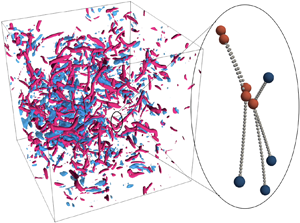
Figure 1. (a) Trajectories of an agglomerate (doublet) and a particle from DNS–DEM simulation. Here,  $1$,
$1$,  $2$ and
  $3$ are initial positions of the particles;
  $1'$,
$1'$,  $2'$ and
  $3'$ are corresponding particles at the collision moment;
  $1''$,
  $2''$ and
  $3''$ are corresponding particles at the end of trajectories. Here, 82 000 collision time steps are used to resolve the process in panel (a), and the position of the particles at each 2000 time steps is presented by a grey sphere. (b) Evolution of the interparticle overlap, where the contacting bond between particle 2 and 3 are formed at
  $\delta _{23} = 0$ (indicated by the vertical dashed line on the left-hand side) and the bonds between particle 2 and 3 and particle 1 and 2 break at
  $\delta _{23} = -\delta _C$ and
  $\delta _{12} = -\delta _C$, indicated by the vertical dashed lines in the middle and on the right-hand side, respectively.
2.4. Identification of collision, rebound and breakage events
The DNS–DEM computational framework is designed with multiple-time steps (Li & Marshall Reference Li and Marshall2007; Marshall Reference Marshall2009). The flow field is updated with a dimensionless fluid time step  $\textrm {d}t_F = 0.005$, which ensures a sufficiently small Courant number. A dimensionless particle convective time step
  $\textrm {d}t_P = 2.5\times 10^{-4}$ is adopted to update the force, velocity and position of particles that do not collide with other particles. Such a small
  $\textrm {d}t_p$ ensures that the distance each particle travels during a time step is only a small fraction of the particle radius so that any possible collision events can be captured. Once a particle collides with other particles during the particle time step, we then recover its information (i.e. its force, velocity and position) to the start of the current particle time step and instead advect it with a dimensionless collision time step
  $\textrm {d}t_C = 6.25\times 10^{-6}$. The value of
  $\textrm {d}t_C$ is small enough to resolve the rapid variation of the deformation within the contact region between touching particles (see figure 1b) (Marshall Reference Marshall2009). All processes, including particle agglomeration, breakage and rearrangement of agglomerates, therefore are automatically accounted for.
Figure 1(a) presents a typical collision-induced breakage event from the DNS–DEM simulation, where a doublet containing particles 1 (P1) and 2 (P2) collides with a third particle (P3) and then breaks into two singlets. The evolutions of interparticle overlap (scaled by the particle radius  $r_p$) between P1 and P2 and that between P2 and P3 are shown in figure 1(b). The vertical dashed lines, from left to right, mark the moment when the contact between P2 and P3 is formed, the bond between P2 and P3 and that between P1 and P2 break. The contact duration
  $\tau$ of each bond thus can be calculated. For instance,
  $\tau _{23}$ in figure 1(b) indicates the contact duration between P2 and P3.
To accurately interpret the breakage mechanism and formulate the breakage rate of agglomerates in turbulence, it is of crucial importance to identify various events in the simulation, including sticking of particles upon collision, rebound, collision-induced breakage and shear-induced breakage of agglomerates. We determine all these events according to the following criteria.
(a) If the contact duration
 $\tau$ between two colliding particles is smaller than a critical value $\tau _C$, we regard it as a rebound event. In this case, there is no agglomerate formed by these two colliding particles. A rebound event normally happens when the collisional velocity is large (Dong et al. Reference Dong, Mei, Li, Shang and Li2018; Fang et al. Reference Fang, Wang, Zhang, Wei, Wu and Sun2019).
(b) If the bond between two colliding particles does not break within
$\tau _C$, we regard it as a sticking collision. An agglomerate is then formed (or grows in size) upon the collision.(c) When a breakage of a certain bond, whose contact duration is larger than
$\tau _C$, leads to the fragmentation of an agglomerate, we regard it as a breakage event. For each breakage case, two different breakage mechanisms are further identified: if the broken agglomerate collideds with other particles right before its breakage, we consider the breakage event as a collision-induced breakage, otherwise, the breakage event is regarded as shear-induced breakage.


To determine the value of  $\tau _C$, we plot the probability distribution of the contact duration
  $\tau$ for the interparticle bonds in two typical cases in double logarithmic coordinates (see figure 2). There is an obvious scale separation between the contact duration in rebound events and breakage events. In the current work, the critical value
  $\tau _C = 0.005$ (indicated by the vertical dashed line) was chosen to separate the rebound events (
 $\tau < \tau _C$) and the breakage events (
 $\tau > \tau _C$). The following quantities thus can be recorded in each simulation run: the number of collisions
  $N_C$; the number of sticking events
  $N_S$; rebound events
  $N_R$; and breakage events
  $N_B$.

Figure 2. Scaled probability distribution of the contact duration  $\tau$ for the interparticle bonds in two typical cases with
  $St = 5.8$ and (a)
  $Ad = 0.64$ and (b)
  $Ad = 6.4$. The vertical dashed line indicates the critical value
  $\tau = \tau _C = 0.005$, which separates the rebound events (
 $\tau < \tau _C$) and the breakage events (
 $\tau > \tau _C$).
3. Results
3.1. Effect of adhesion on breakage
In figure 3(a–c), we show the temporal evolution of the number of overall collisions  $N_C$, the number of sticking collisions
  $N_S$, rebound events
  $N_R$ and breakage events
  $N_B$ for
  $St = 5.8$ and three different values of adhesion parameter
  $Ad_n$, which is defined as
 \begin{equation} Ad_n = \frac{\gamma}{\rho_p \bar{v}_{n}^2 r_p}, \end{equation}
where  $\bar {v}_{n} = \sqrt {\langle v_n^{2}\rangle }$ is the square root of the average value of
  $v_n^{2}$ over all collision events. The particles are considered to have collided at the minimum separation distance
  $h = h_{min} = 2 \times 10^{-4} r_p$ and the impact velocity
  $v_n$ is calculated for each collision event at this moment. The values of
  $v_n$ are different for different collision events and
  $\bar {v}_{n}$ here can be regarded as an effective value to measure the kinetic energy of colliding particles. When the adhesion is extremely weak (
 $Ad_n = 0.73$),
  $N_C$ increases linearly with time. It indicates that the collision kernel
  $\varGamma$ almost keeps as a constant, which is consistent with previous DNS results for non-adhesive particles (Wang et al. Reference Wang, Wexler and Zhou2000). Here,
  $N_R$ is close to
  $N_C$ and both
  $N_S$ and
  $N_B$ are nearly zero. Agglomerates therefore can barely be formed given such a weak adhesion. For the case with a relatively stronger adhesion (
 $Ad_n = 7.3$), agglomeration between colliding particles can be clearly observed. However, the agglomeration at this
  $Ad_n$ value is still quite limited, since the sticking probability is small (
 ${\sim }0.4$). When
  $Ad_n$ further increases to
  $70$, adhesion plays a dominant role. As illustrated in figure 3(c),
  $N_S \approx N_C$, implying that almost all collisions lead to the agglomeration of colliding particles. Moreover,
  $N_C$ no longer increases linearly with time in this case, which confirms previous results that intense agglomeration will push the system away from statistical equilibrium.

Figure 3. Temporal evolution of the number of collisions  $N_C$, the number of sticking collisions
  $N_S$ and rebound collisions
  $N_R$, and the number of breakage events
  $N_B$ for
  $St = 5.8$ and
  $(a)$
$(a)$ $Ad_n = 0.73$,
  $(b)$
$(b)$ $Ad_n = 7.3$ and
  $(c)$
$(c)$ $Ad_n = 70$.
Another interesting result observed in figure 3 is that the breakage of agglomerates is not obvious when the adhesion is either too weak or too strong. When  $Ad_n = 0.73$, the breakage is limited by the small number of bonds that can be formed upon collisions. In contrast, the contacting bond formed at
  $Ad_n = 70$ is too strong to be broken by the fluid stress or the impact of a third particle. A considerable number of breakage events can only be observed at a moderate value of
  $Ad_n$.
We normalize the number of sticking collisions  $N_S$, rebound collisions
  $N_R$ and breakage events
  $N_B$ with the total number of collisions
  $N_C$ and plot them against
  $Ad_n$ in figure 4. Three different regimes can be identified: a rebound regime with
  $\hat {N}_R > 95\,\%$; a sticking regime with
  $\hat {N}_S > 95\,\%$; and a transient regime between the above two regimes. The critical
  $Ad_n$ values dividing the three regimes are approximately
  $1.5$ and
  $35$. Simulation results for different
  $St$ collapse, implying that the possibility of occurrence of sticking, rebound and breakage events can be well quantified by the dimensionless adhesion number
  $Ad_n$.

Figure 4. Normalized number of sticking collisions  $\hat {N}_S$ (blue), rebound collisions
  $\hat {N}_R$ (red) and breakage events
  $\hat {N}_B$ (purple) over the entire simulation as functions of
  $Ad_n$. Results for three different Stokes numbers are shown: circles,
  $St = 2.9$; triangles,
  $St = 5.8$; and diamonds,
  $St = 12$.
3.2. Formulation of breakage rate
In the current subsection, we focus on the formulation of the rate of collision-induced breakage of agglomerates. In turbulent flow laden with particles, the growth or collision-induced breakage of agglomerates results from two successive processes. First, the turbulent flow brings two initially separate agglomerates (or particles) close enough to initiate collisions. Second, the two colliding agglomerates will either merge into a large one, rebound from each other or break up into fragments.
For the first step (i.e. collision), we introduce the classic statistical model of the collision rate in particle-laden turbulence. The collision rate for agglomerates of size  $i$,
$i$,  $\dot {n}_{C}(i)$, can be expressed as
 \begin{equation} \dot{n}_{C}(i)= \sum_{j=1}^{\infty} \varGamma(i, j) n(j)n(i), \end{equation}
where  $\varGamma (i,j)$ is the collision kernel between agglomerates of size
  $i$ and agglomerates of size
  $j$ and
  $n(i)$ is the average number concentration of size group
  $i$. For homogenous isotropic turbulence, the collision kernel
  $\varGamma (i, j)$ has been modelled by (Zhou, Wexler & Wang Reference Zhou, Wexler and Wang2001)
 \begin{equation} \varGamma(i, j)=2 {\rm \pi}R_{i j}^{2}\left\langle\left|w_{r}\right|\right\rangle g\left(R_{i j}\right), \end{equation}
where  $R_{ij}$ is the radius of the effective collision spheres (known as ECSs) for agglomerates of size
  $i$ and
  $j$,
$j$,  $\langle |w_{r}|\rangle = \bar {v}_n$ is the average radial relative velocity and
  $g(R_{ij})$ is the radial distribution function at the distance of contact. The collision kernel
  $\varGamma (i,j)$ has been evaluated for non-interacting particles with different values of Stokes number in several previous studies. For monodisperse spherical particles (i.e.
  $i=j=1$), the collision kernel, normalized by the collision kernel for zero-inertia particles
  $\varGamma _0 (1,1) =(8 {\rm \pi}\epsilon / 15 v)^{1 / 2}(2 r_{p})^{3}$, increase from
  $1$ to
  ${\sim }10$ as
  $St$ increase from
  $0$ to
  ${\sim }1$ and does not obviously change when
  $St$ further increases (Saffman & Turner Reference Saffman and Turner1956; Sundaram & Collins Reference Sundaram and Collins1997; Wang et al. Reference Wang, Wexler and Zhou2000; Zhou et al. Reference Zhou, Wexler and Wang2001). In our simulation, the values of
  $\varGamma (1,1) / \varGamma _{0}(1,1)$ are
  $7.0$,
  $10.2$,
  $11.1$,
  $11.0$ for
  $St = 1.4, 2.9, 5.8$,
  $12$, respectively. These values are quite close to the previous DNS results for non-interacting particles (Wang et al. Reference Wang, Wexler and Zhou2000). The effective collision radius for an agglomerate with
  $i$ primary particles and that with
  $j$ primary particles can be calculated as
  $R_{ij}=R_g(i)+R_g(j)$, where
  $R_g(i)$ is the gyration radius for the agglomerates with
  $i$ primary particles (Jiang & Logan Reference Jiang and Logan1991; Flesch, Spicer & Pratsinis Reference Flesch, Spicer and Pratsinis1999; Chen et al. Reference Chen, Li and Marshall2019a).
The breakage rate due to the collisions with other particles or agglomerates can be expressed as the product of the collision rate  $\dot {n}_{C}(i)$ and the fraction of collision events resulting in breakage
  $\varPsi$ (Kellogg et al. Reference Kellogg, Liu, LaMarche and Hrenya2017) as follows:
 \begin{equation} f_{br}(i) = \frac{\varPsi \dot{n}_{C}(i)} {n(i)} = \varPsi \sum_{j=1}^{\infty} \varGamma(i, j) n(j). \end{equation}
 Here, the fraction of breakage events  $\varPsi$ is defined as the ratio of the breakage number to the overall collision number and should include the influence of both turbulent transport and particle scale interactions. In prior work, a critical breakage velocity
  $v_{b,crit}$ was introduced, assuming that agglomerate breaks when the magnitude of the normal relative velocity
  $v_n$ satisfies
  $v_n > v_{b,crit}$. The fraction of breakage events
  $\varPsi$, therefore, can be calculated as
  $\varPsi =\int _{v_{b, {crit}}}^{\infty } P_C(v_{n})\,\textrm {d} v_{n}$, with
  $P_C(v_n)$ being the probability density function (p.d.f.) of normal impact velocity (Kellogg et al. Reference Kellogg, Liu, LaMarche and Hrenya2017; Liu & Hrenya Reference Liu and Hrenya2018). Here, we introduce a new statistical framework to calculate
  $\varPsi$ in terms of well known impact velocity distributions
  $P_C(v_n)$. This formulation is expected to be more general than the previous model based on the critical breakage velocity. For collision events with impact velocity
  $v_n$, the fine-grained probability of breakage is recorded as
  $\psi (v_n)$. Thus, the distribution of velocity for a breakage event is given by
 \begin{equation} P_B(v_n)=\frac{P_C(v_n) \psi\left(v_{n}\right)}{\int_0^{\infty} P_C(v) \psi\left(v\right)\, \mathrm{d} v}, \end{equation}
where the denominator is the normalization coefficient. Here,  $\psi (v)$ can be regarded as a transfer function, which relates the probability distribution of breakage to the impact velocity distribution.
For particles with a given adhesion value,  $\psi (v_n)$ is expected to be zero as
  $v_n$ tends to zero (sticking regime), and rises to unity as
  $v_n$ increases, given that all colliding agglomerates will break when the impact velocity is sufficiently large. Knowing the value of
  $\psi (v_n)$, one can directly obtain the fraction of breakage
  $\varPsi$ through
 \begin{equation} \varPsi = \int_0^{\infty} P_C(v_n) \psi\left(v_n\right)\, \mathrm{d} v_n. \end{equation}
Substituting (3.6) into (3.4) further gives the breakage rate.
To validate the statistical framework above and to give a specification of the transfer function  $\psi (v_n)$, we obtain the statistics of doublet breakage from DNS–DEM simulation and compare them with the theoretical descriptions in (3.4). The breakage of doublets has been widely adopted as the prototype of agglomerates that break into two fragments. For doublets, the breakage rate in (3.4) reduces to
 \begin{equation} f_{br}(2) = \frac{\varPsi \dot{n}_{C}(2)}{n(2)} = \varPsi \sum_{j=1}^{\infty} \varGamma(2, j) n(j). \end{equation}
At the early stage of agglomeration most particles remain as singlets (Liu & Hrenya Reference Liu and Hrenya2018; Chen et al. Reference Chen, Li and Marshall2019a) and the equation above can be further simplified as
 \begin{equation} f_{br}(2) \approx \varPsi \varGamma(1, 2) n(1) = n(1)S_{12} \varPsi \varGamma(1,1). \end{equation}
On the right-hand side of the equation, we relate the singlet–doublet collision kernel  $\varGamma (1,2)$ to the singlet–singlet kernel through
  $\varGamma (1,2) = S_{12}\varGamma (1,1)$, where the constant
  $S_{12}$ is the correction for collisional cross-sectional areas for singlet–doublet collisions. Here,
  $\varGamma (1,1)$ for particles with different
  $St$ values has been well modelled from the ghost particle approach. Although the expression in (3.8) only gives low-order statistics for the breakage of doublets, it provides valuable insights: the breakage rate scale linearly to the number concentration and the effect of turbulent transport are included in both
  $\varGamma (1,1)$ and the breakage fraction
  $\varPsi$; contacting interactions affects the breakage rate by changing
  $\varPsi$ through the transfer function
  $\psi (v_n)$ in (3.6).
In order to obtain the transfer function  $\psi (v_n)$, we track all the collision events in the simulation and record whether the collision leads to the breakage of the agglomerate according to the criterion in § 2.4. The p.d.f. of the impact velocity
  $P_C(v_n)$ for singlet–doublet collision events are then measured at different
  $St$ and
  $Ad$ values (as shown in figure 5a–c). For the cases with weak adhesion (
 $Ad = 0.64$), most particles remain as singlets and the number of singlet–doublet collision events that can be observed within a large-eddy turnover time is quite limited. We thus run three simulations with different initial random positions of particles to obtain more collision events. It ensures a good statistic on the collision velocity for singlet–doublet collision events and breakage events. For a given value of
  $St$, varying
  $Ad$ does not obviously affect
  $P_C(v_n)$. In contrast, a strong dependence on
  $St$ can be observed. For collisions that result in the breakage of a doublet, we also plot the corresponding p.d.f. of the impact velocity,
  $P_B(v_n)$, in figure 5(d–f). One can easily find a strong correlation between
  $P_B(v_n)$ and
  $Ad$. Particles with stronger adhesion tend to stick together upon collisions. The breakage events, therefore, are more likely to happen with a higher impact velocity.

Figure 5. Probability density functions of the collision velocity (normal component)  $v_n$ for singlet–doublet collision events (a–c) and collision-induced breakage events (d–f). Statistics are made over approximately a large-eddy turnover time
  $t\in [15, 25]$. Different columns are results for different Stokes numbers:
  $St = 2.9$ (a,d);
  $St = 5.8$ (b,e); and
  $St = 12$ (c,f). For each Stokes number, we show results from different
  $Ad$ values:
  $Ad = 0.64$ (squares);
  $Ad = 1.3$ (circles);
  $Ad = 6.4$ (upward triangles); and
  $Ad = 12$ (downward triangles).
We then calculate the transfer function  $\psi (v_n)$ inversely from
  $P_C(v_n)$ and
  $P_B(v_n)$ according to (3.5). As shown in figure 6(a), despite the inconsistency in
  $P_C(v_n)$,
  $\psi (v_n)$ for different
  $St$ collapses nicely. In contrast, the adhesion strongly affects
  $\psi (v_n)$. Although, there is considerable scatter in the data at large
  $v_n$ due to the limited sample size of the energetic collision events, the transfer function
  $\psi (v_n)$ at a given
  $Ad$ value is roughly linear to the collision velocity
  $v_n$. The results in figure 6(a) suggest that the transfer function may only depend on the short-range contacting interactions, whereas the effects of turbulent transport and hydrodynamic interactions are included in the p.d.f. of the impact velocity
  $P_C(v_n)$. To validate the argument above, we run simulations with different particle radius (ranging from 0.0075 to 0.0125) and with/without the hydrodynamic damping force (2.5) at a fixed
  $St$ value. As seen in figure 6(a), the measured transfer function
  $\psi (v_n)$ does not show obvious dependence on the particle size and the hydrodynamic interaction, confirming that the transformation function
  $\psi (v_n)$ is determined by the short-range contacting interactions.

Figure 6. (a) Transfer function  $\psi (v_{{n}})$ versus collision velocity
  $v_n$ for different Stokes numbers:
  $St = 2.9$ (squares);
  $5.8$ (circles); and
  $12$ (triangles). Also for different
  $Ad$ values:
  $Ad = 1.3$ (light blue);
  $6.4$ (yellow); and
  $12$ (dark blue). Results with different particle radius (ranging from 0.0075 to 0.0125) and with/without the hydrodynamic damping force (2.5) at
  $St = 2.9$ are also included. Scatters are results calculated from p.d.f. in figure 5, and dashed lines are linear fittings from (3.9). (b and c) Fitting parameters
  $(v_{C2} - v_{C1})^{-1}$ and
  $v_{C1}$ as functions of
  $Ad$. Legends are the same as in panel (a).
According to the results in figure 6(a), we propose a linear relationship between  $\psi$ and
  $v_n$ as follows:
 \begin{equation} \psi(v_n)=\begin{cases} {0,} & {\text{for } v_n < v_{C1},} \\ {\dfrac{1}{v_{C2} - v_{C1} } (v_n - v_{C1}),} & {\text{for } v_{C1} \leq v_n \leq v_{C2},}\\ {1,} & {\text{for } v_n > v_{C2}.} \end{cases}\end{equation}
Two typical values of collision velocity  $v_{C1}$ and
  $v_{C2}$ are indicated by (3.9). Breakage does not happen when the collision velocity between two agglomerates,
  $v_n$, is smaller than
  $v_{C1}$. On the other hand, if
  $v_n > v_{C2}$, the colliding doublets always break. We then fit the measured values of the transfer function
  $\psi (v_n)$ (linear part) using (3.9) for all the cases presented in figure 6(a) and plot the fitting parameters
  $v_{C1}$ and the slope
  $(v_{C2} - v_{C1})^{-1}$ as a function of
  $Ad$. It is seen that the fitted values of the slope for different cases centre around a logarithmic curve (figure 6b), which reads
 \begin{equation} (v_{C2} - v_{C1})^{-1} = -2.1 \ln \left( \frac{Ad}{13}\right). \end{equation}
Several interesting features are indicated by (3.10). First, the slope diverges in the small adhesion limit ( $Ad \to 0$), indicating that there is a critical collision velocity separating the breakage and non-breakage collisions. This is in accordance with the theoretical model proposed by Liu & Hrenya (Reference Liu and Hrenya2018), in which a Heaviside function
  $H(v - v_{b,crit})$ is proposed to transform the p.d.f. of normal impact velocity
  $P_C(v_n)$ into the p.d.f. of impact velocity for breakage events
  $P_B(v_n)$. We show here that such a transfer function is reasonable only when the adhesive interaction is extremely weak. As
  $Ad$ increases, the slope of
  $\psi (v_n)$ considerably decreases and there is no sharp transition between breakage and non-breakage collision velocities. Although the data points for the minimum breakage velocity
  $v_{C1}$ are relatively dispersed when plotted as a function of
  $Ad$, a quadratic curve,
  $v_{C1} = a\,Ad^2$ with
  $a = 7.4\times 10^{-4}$, can roughly describe the variation of
  $v_{C1}$ (see figure 6c). At large adhesion limit
  $v_{C1}$ diverges, implying that all collisions give rise to the growth of agglomerates when the adhesion is sufficiently strong.
To further validate the model of the transfer function, we present an example of the model prediction for cases with  $St= 2.9$ in figure 7(a). First, the p.d.f. of the normal collision velocity
  $P_C(v_n)$ is measured from the simulation with small
  $Ad$ value (
 $1.3$). The breakage fraction
  $\varPsi$ is then calculated by substituting (3.9) and the measured
  $P_C(v_n)$ into (3.6). One can also adopt models of
  $P_C(v_n)$ obtained from simulations with non-interacting particles to estimate the breakage fraction
  $\varPsi$ (Salazar & Collins Reference Salazar and Collins2012; Saw et al. Reference Saw, Bewley, Bodenschatz, Ray and Bec2014; Bhatnagar, Gustavsson & Mitra Reference Bhatnagar, Gustavsson and Mitra2018). Such approximation does not bring large errors since
  $P_C(v_n)$ is almost independent of adhesive interactions (see figure 5). The result generated from the model together with predictions for
  $St = 1.4$,
  $5.8$ and
  $11.5$ is plotted as a dashed line in figure 7(b). We see that the model predictions are in accordance with DNS–DEM simulations.

Figure 7. (a) Probability density functions  $P_C(v_n)$ of the normal collision velocity for
  $St = 2.9$ and
  $Ad = 1.3$ (left-hand axis) and the transfer function
  $\psi (v_n)$ modelled by (3.9) (right-hand axis). Colour code spans from blue to yellow with increasing
  $Ad$ (from
  $0.1$ to
  $10$). (b) Fraction of collision-induced breakage of doublets
  $\varPsi$ at different
  $Ad$ values. Points are DNS–DEM results and dashed lines are results calculated from
  $P_C(v_n)$ and the modelled
  $\psi (v_n)$ (3.9).
The deviation between the model and the simulations in figure 7(b) may result from the linear assumption of the transfer function  $\psi (v_n)$ (3.9), in which a sharp transition is assumed between the linear part
  $((v_n-v_{C1})/(v_{C2}-v_{C1}))$ and unity. The simulation data in figure 6(a), in contrast, shows a much slower approach to unity, indicating that the model in (3.9) overestimates
  $\psi (v_n)$ when
  $v_n \to v_{C2}$. Despite this deviation, our simplified model well captures the variation of breakage fraction
  $\varPsi$ with adhesion
  $Ad$. Moreover, the Stokes number dependence of
  $\varPsi$ can be observed in figure 7(b). Since the breakage fraction
  $\varPsi$ here is calculated from a universal transfer function, the
  $St$ number dependence of
  $\varPsi$ originates from the difference in
  $P_C(v_n)$: the hydrodynamic damping force significantly reduces the relative approaching velocity of colliding particles with small
  $St$.
$St$.
The collision-induced breakage rate of the doublets  $f_{b r}(2)$ is calculated from (3.8) and compared with DNS–DEM results in figure 8(a). Quantitative agreement is observed, indicating that the analytical model well captures the effects of the particle inertia and the adhesive interaction on the breakage. Since the adhesion parameter
  $Ad$ does not include the effect of particle inertia, there is considerable distinction in results for different
  $St$ at the same
  $Ad$. We stress again that particle inertia affects the breakage rate through its influence on the statistics of the collision velocity. One simple way to include both effects of particle inertia and the adhesion is to use the modified adhesion parameter
  $Ad_{n}$ (see (3.1)), which scales the adhesion using
  $St$-dependent average velocity
  $\bar {v}_{n} = \sqrt {\langle v_n^{2}\rangle }$. The normalized breakage rate, when plotted as a function of
  $Ad_{n}$, collapses nicely onto the exponential curve (see figure 8b)
 \begin{equation} \frac{f_{br}\tau_k}{r_p^3 n(1)} = 86\exp(-0.12Ad_n). \end{equation}
The result indicates that  $\bar {v}_{n} = \sqrt {\langle v_n^{2}\rangle }$ is an appropriate choice to scale the effect of adhesion and the collision-induced breakage rate can be well estimated once
  $Ad_n$ is known.

Figure 8. (a) Normalized breakage rate  $f_{br}\tau _k/(r_p^3 n(1))$ for doublets as a function of
  $Ad$. The scatters are DNS–DEM results and the dashed lines are predictions from (3.8), in which the breakage fraction
  $\varPsi$ is calculated from the p.d.f. of normal collision velocity through
  $\varPsi =\int _{0}^{\infty } P_{C}(v_n) \psi (v_n) \,\mathrm {d} v$ (see (3.6)) and the transfer function
  $\psi (v_n)$ is modelled by (3.9). (b) Normalized breakage rate as a function of
  $Ad_n$. The dashed line is exponential fittings using (3.11).
It should be noted that the model in (3.8) is valid only for early stage agglomeration, since the transfer function is derived for singlet–doublet collisions. Both agglomerate size and structure may affect the formulation of the transfer function. Predicting the breakage rate for agglomerates with arbitrary size and structures through first principles is practically impossible. It is thus normally accepted to describe the breakage rate using an exponential or a power-law function, in which the parameters are related to agglomerate size and particle–particle interactions. Agglomerate size dependence of the breakage rate will be discussed in § 3.3.
It is of great importance to know how the breakage rate scales with particle size  $r_p$ and particle number density
  $n$. We measure the doublet breakage at different particle sizes (
 $r_p = 0.005\text {--}0.015$) and particle numbers (
 $N = 19\,600\text {--}40\,000$) for typical
  $St$ and
  $Ad$ values (shown in figure 9). The results are plotted in a scaled form:
  $\hat {f}_{br} = f_{br}(r_p)/f_{br}(r_{p,0})$,
  $\hat {r}_p = r_p/r_{p,0}$ in figure 9(a) and
  $\hat {f}_{br} = f_{br}(n(1))/f_{br}(n_{m}(1))$,
  $\hat {n}(1) = n(1)/n_{m}(1)$ in figure 9(b). Here,
  $f_{br}(r_{p,0})$ is the doublet breakage rate for the case with
  $r_{p,0} = 0.01$ and
  $f_{br}(n_{m}(1))$ is the breakage rate for the case with the maximum value of singlet number density
  $n_{m}(1)$. As displayed in figure 9, DNS–DEM results follow the power laws
  $\hat {f}_{br} \propto \hat {r}^2_p$ and
  $\hat {f}_{br} \propto \hat {n}^1(1)$ when particle size and singlet number density are varied.

Figure 9. Scaled breakage rate  $\hat {f}_{br}$ as a function of (a) scaled particle size
  $\hat {r}_p$ and (b) scaled number density of singlet
  $\hat {n}(1)$ at
  $St = 2.9$,
  $5.8$
$5.8$ $12$ and
  $Ad = 1.3$,
  $3.8$. Dashed lines in (a and b) indicate power law functions with exponents
  $2$ and
  $1$, respectively.
The  $n(1)$ dependence is easy to understand from (3.8). The
  $\hat {r}^2_p$ scaling originates from the
  $r_p$ dependence of the collision kernel
  $\varGamma (1,1)$ in (3.8). For inertial particles (
 $St \gg 1$), the approaching velocity of colliding particles is decorrelated from the local fluid gradient, thus is not affected by the particle size. The
  $\hat {r}^2_p$ scaling enters
  $\varGamma (1,1)$ through the effective collision area. We note that the size scaling here is valid for particles that are smaller than or comparable to the Kolmogorov scale. It may not hold for particles that are considerably larger than the Kolmogorov scale. In the latter case, particle-resolved simulations would be needed to precisely calculate the flow around and forces on particles (Ernst, Dietzel & Sommerfeld Reference Ernst, Dietzel and Sommerfeld2013; Liu & Wu Reference Liu and Wu2019; Peng, Ayala & Wang Reference Peng, Ayala and Wang2019; Wang et al. Reference Wang, Wan, Peng, Liu and Wang2019).
3.3. Agglomerate size dependence of the breakage rate
The breakage rate of agglomerates with size  $A$ are calculated from DNS–DEM simulations according to
 \begin{equation} f_{br}(A) = \frac{N_{br}(A)}{N(A)\Delta t}, \end{equation}
where  $N(A)$ is the number of agglomerates of size A averaged over the time range
  $t\in [30,40]$,
  $N_{br}(A)$ is the breakage number of agglomerates with size
  $A$ and
  $\Delta t = 10$. As shown in figure 10(a), a stronger adhesion promotes the formation of larger agglomerates. In contrast, the number of breakages decreases with
  $Ad$ (see figure 10b). To provide meaningful statistics, we only calculate
  $f_{br}(A)$ when
  $N_{br}(A)$ is larger than
  $20$. The results are normalized by the mean shear rate
  $G$ and plotted as a function of size
  $A$ in figure 10(c). It is seen that the breakage rate depends linearly on the agglomerate size with the slope being a function of
  $Ad_n$. Fitting the data at different
  $Ad_n$ and
  $St$ according to
 \begin{equation} \frac{f_{b r}(A)}{G}=\zeta(St, Ad_n)\, A +\chi \end{equation}
gives us the values of the slope  $\zeta (St,Ad_n)$. As shown in figure 10(d), when plotted as a function of
  $Ad_n$,
  $\zeta$ for different
  $St$ centres around a universal curve, which is analogous to the
  $f_{br}$ dependence in figure 8(b). The universal curve has an power-law form:
  $\zeta = 0.012Ad_n^{-0.81}$. These results once again confirm that the modified adhesion parameter
  $Ad_n$ is an appropriate choice to reflect both effects of the particle inertia and adhesive interactions on the breakage.

Figure 10. (a) Number of agglomerates of size  $A$ averaged over the time range
  $t\in [30,40]$. (b) Number of breakages of agglomerates of size
  $A$ measured within
  $t\in [30,40]$ for
  $St = 5.8$. (c) Breakage rate, normalized by the shear rate
  $G$, as a function of agglomerate size
  $A$. The dashed lines are linear fittings from (3.13). (d) The fitting values of the slope
  $\zeta$ for the linear relationship between
  $f_{br}/G$ and
  $A$ at different
  $Ad_n$ and
  $St$ values. The dashed line indicates the power function
  $\zeta = 0.012Ad_n^{-0.81}$.
3.4. Role of flow structure
In this subsection, we quantify the correlation between structures of turbulence and the breakage of agglomerates with different  $St$ and
  $Ad$ values. We identify the flow structures based on the second invariant of the velocity gradient tensor
  $\mathcal {Q}=(\mathcal {R}^{2}-\mathcal {S}^{2}) / 2$, where the strain rate tenor
  $\mathcal {S}=(\mathcal {A}+\mathcal {A}^{\mathrm {T}}) / 2$ and the rotation rate tensor
  $\mathcal {R}=(\mathcal {A}-\mathcal {A}^{\mathrm {T}}) / 2$ are symmetric and antisymmetric parts of the velocity gradient tensor
  $\mathcal {A}=\tau _{k} \boldsymbol {\nabla } \boldsymbol {u}$ (normalized by the Kolmogorov time
  $\tau _{k}$), respectively. Figure 11(a) presents the countour plots of
  $Q$, showing the vortex tubes with
  $Q > 3.3\sqrt {\langle Q^2 \rangle }$ and straining sheets with
  $Q < -2.5\sqrt {\langle Q^2 \rangle }$, and the corresponding two-dimensional slice at
  $y=0$. One can clearly see the red vortex tubes surrounded by blue straining sheets (vortex-strain worm-rolls), which implies that intense structures typically occur near each other (Picardo et al. Reference Picardo, Agasthya, Govindarajan and Ray2019).

Figure 11. (a) Countour plot of  $Q$ and the two-dimensional slice at
  $y=0$. Vortex tubes with
  $Q > 3.3\sqrt {\langle Q^2 \rangle }$ are coloured in red and straining sheets with
  $Q <-2.5\sqrt {\langle Q^2 \rangle }$ are coloured in blue. (b) Average
  $Q$, sampled by singlet–doublet collision events and (c) average
  $Q$ sampled by doublet breakage events as functions of
  $St$. (d) Average
  $Q$ for breakage events as a function of
  $Ad$ at different
  $St$ values:
  $St= 1.4$ (squares);
  $St = 2.9$ (circles);
  $St = 5.8$ (upward triangles); and
  $St = 12$ (downward triangles). The straight dashed lines are linear fittings.
We calculate the average  $\mathcal {Q}$, sampled by singlet–doublet collisions, at different
  $St$ and
  $Ad$ values in figure 11(b). The results for non-interacting particles based on ghost collision approximations are also included (Picardo et al. Reference Picardo, Agasthya, Govindarajan and Ray2019) (only data at
  $St > 0.5$ are shown here). One can notice that as
  $St$ increases from
  $0.5$ to
  $20$,
$20$,  $\mathcal {Q}$ increases from a negative value to zero, implying that finite-inertia particles (
 $St\sim 1$) tend to collide in the straining zone whereas particles with large inertia collide uniformly. According to Picardo et al. (Reference Picardo, Agasthya, Govindarajan and Ray2019), decreasing
  $St$ also leads to the approach to zero of
  $\mathcal {Q}$ and the largest absolute value of
  $\mathcal {Q}$ occurs at
  $St \approx 0.3$. Such flow structure dependence is due to two aspects. First, particles with finite inertia (
 $St \approx 1$) tend to accumulate in straining regions outside vortices due to the centrifugal effect (known as preferential concentration). Moreover, particle inertia also increases the relative approaching velocity between particles. Such an effect also prevails in straining zones (Picardo et al. Reference Picardo, Agasthya, Govindarajan and Ray2019). Here, we show that varying particle–particle contacting interactions (
 $Ad$) does not obviously affect the structure dependence of collisions.
The average  $\mathcal {Q}$, sampled by singlet–doublet collision-induced breakage events, shows a strong dependence on
  $Ad$ (figure 11c). Doublets with larger
  $Ad$ value are more difficult to break thus needing higher impact velocities. For particles with moderate inertia (
 $St \approx 1$), violent collisions are more likely caused by particles ejected rapidly from strong vortices and happen in straining sheets (with smaller negative
  $\mathcal {Q}$) that envelope the vortices. As
  $St$ increases, the relative velocity between colliding particles becomes less sensitive to the underlying flow, both collision events and breakage events distribute more uniformly in the flow. As shown in figure 11(d), the relationship between
  $\mathcal {Q}$ and
  $Ad$ at given
  $St$ can be well described by linear functions.
4. Discussion and conclusions
By means of DNS and multiple time scale DEM, we are able to resolve all the collision, rebound and breakage events for adhesive particles in turbulence. We have shown that the collision-induced breakage rate of agglomerates can be modelled based on the statistics of the collision rate and a breakage fraction function  $\varPsi$. A scaling relationship of the breakage rate for doublets at the early stage is proposed, which includes the effects of particle size, turbulent transport and particle number concentration. The fraction function
  $\varPsi$ is further expressed as a function of the well known distributions of impact velocity and a universal transfer function
  $\psi (v_n)$, which are shown to rely on particle–particle contacting interactions and are independent of particle inertia
  $St$, particle size and hydrodynamic interactions. Based on a large number of simulations, we propose an exponential function of adhesion parameter
  $Ad_n$ for the breakage rate of doublets and show that the breakage rate increases linearly as the agglomerate size increases. The framework allows one to estimate the breakage rate for early stage agglomerates of arbitrary size.
It is of great interest to compare our results with shear-induced breakage of agglomerates, which has been extensively investigated for both isostatic loose agglomerates (De Bona et al. Reference De Bona, Lanotte and Vanni2014) and dense ones. The shear-induced breakup rate for doublets scales exponentially with a dimensionless parameter,  $\mathcal {N}$ (De Bona et al. Reference De Bona, Lanotte and Vanni2014),
 \begin{equation} f_{br}^{sh}= \frac{k_{f}}{\tau_{k}} \exp (-\alpha \mathcal{N}), \end{equation}
where  $\mathcal {N}=F_{C} /(6 {\rm \pi}\mu r_p^{2} {G}_{{eff}})$,
  $F_{C}$ is the strength of the bond and
  $6 {\rm \pi}\mu r_p^{2} G_{{eff}}$ estimates the largest tensile stress acting on the bond by the flow field with an effective shear rate
  ${G}_{{eff}}$. Here,
  $k_{f}$ is a prefactor of order unity and
  $\alpha$ is fitted to be
  $4.8$ for
  $\mathcal {N} <0.5$ and
  $1.8$ for
  $\mathcal {N} > 1.5$. According to (3.11) and (4.1), the ratio between collision-induced breakage rate
  $f_{br}^{co}$ and shear-induced breakage rate
  $f_{br}^{sh}$ can be estimated as
 \begin{equation} \frac{f_{b r}^{s h}}{f_{b r}^{c o}} \sim \phi^{-1} \frac{\exp \left(-0.25\alpha \gamma r_{p}^{-1} \mu^{-1} {G}_{{eff}}^{-1} \right)}{\exp (-0.12 Ad_n)} = \phi^{-1} \frac{\exp \left(-0.25\alpha Ad_{sh} \right)}{\exp (-0.12 Ad_n)}, \end{equation}
where  $\phi$ is the volume fraction of particles. The numerator in (4.2) is rearranged to form an adhesion parameter
  $Ad_{sh}$, which measures the relative importance of adhesion and the shear stress. The parameter
  $Ad_{sh}$ has been successfully used to predict whether an agglomerate exposed to the simple shear flow will break or not (Ruan et al. Reference Ruan, Chen and Li2020). Given the parameters in our simulation conditions, we have
  $f_{br}^{sh}/f_{br}^{co} \ll 1$, indicating that shear-induced breakage can be neglected in the current work. However, increasing the effective shear rate (
 $G_{{eff}}$) and decreasing the volume fraction (
 $\phi$) of the particles can both magnify the relative importance of shear-induced breakage. Given (4.2), it is straightforward to determine the dominant breakage mechanism. Our results extend those of Seto et al. (Reference Seto, Botet and Briesen2011), Vanni & Gastaldi (Reference Vanni and Gastaldi2011), Fellay & Vanni (Reference Fellay and Vanni2012), De Bona et al. (Reference De Bona, Lanotte and Vanni2014) and Bäbler et al. (Reference Bäbler, Biferale, Brandt, Feudel, Guseva, Lanotte, Marchioli, Picano, Sardina and Soldati2015), which focus on the breakage of agglomerates due to hydrodynamic stresses, forming a more complete picture of breakage in turbulent flows.
In the present work, we have also shown that for adhesive particles with moderate inertia ( $St\approx 1$), the breakage events are more likely caused by particles ejected from strong vortices and happen in strain regions. It should be noted that the Reynolds number
  $Re_{\lambda }$ currently used in the DNS–DEM simulation is fixed as
  $93$, which is a modest value. Higher
  $Re_{\lambda }$ results in stronger intermittency and more intense vortex and strain structures, which give rise to extremely high impact velocities. Such intense structures, however, occupy smaller volumes as
  $Re_{\lambda }$ increases (Picardo et al. Reference Picardo, Agasthya, Govindarajan and Ray2019). These competing effects would cause a non-monotonic variation of the breakage rate. For heavy particles with
  $St \ge 10$, the radial relative velocity increases with
  $Re_{\lambda }$ since the particles carry a memory of more energetic motions as
  $Re_{\lambda }$ increases. Such an effect is expected to increase the collision-induced breakage rate according to (3.8). Other effects, including the correlated and extreme collision events (Bec et al. Reference Bec, Ray, Saw and Homann2016; Saw et al. Reference Saw, Kuzzay, Faranda, Guittonneau, Daviaud, Wiertel-Gasquet, Padilla and Dubrulle2016) and multifractal statistics of velocities differences (Saw et al. Reference Saw, Bewley, Bodenschatz, Ray and Bec2014), appear in high-Reynolds-number flows may also contribute to the breakage rate. A complete picture of agglomeration and breakage, therefore, should include the role of both the turbulent transport and particle-level interactions, which will be systematically investigated in future studies.
Acknowledgements
S.Q.L. acknowledges support from the National Natural Science Foundation of China (grant no. 51725601). We are grateful to Professor F. Toschi at Technische Universiteit Eindhoven, Marshall, Professor J. Marshall at Vermont and Professor E. Climent at Université de Toulouse for fruitful discussions, and Professor C. Sun and Mr Ruan at Tsinghua University for their useful suggestions.
Declaration of interests
The authors report no conflict of interest.


