2.1 Looijenga pairs

Let $(Y,D)$ be a Looijenga pair:Footnote ⁴ $Y$ is a smooth projective complex surface and $D$ is a singular reduced normal crossings anticanonical divisor on $Y$. Writing the irreducible components

$$\begin{eqnarray}D=D_{1}+\cdots +D_{r},\end{eqnarray}$$

$D$ is a cycle of $r$ irreducible smooth rational curves $D_{j}$ if $r\geqslant 2$, or an irreducible nodal rational curve if $r=1$. The complement $U:=Y-D$ is a non-compact Calabi–Yau surface, equipped with a holomorphic symplectic form $\unicode[STIX]{x1D6FA}_{U}$, defined up to non-zero scaling and having first-order poles along $D$. We refer to [Reference LooijengaLoo81, Reference FriedmanFri15, Reference Gross, Hacking and KeelGHK15a, Reference Gross, Hacking and KeelGHK15b] for more background on Looijenga pairs.

There are two basic operations on Looijenga pairs:

1. – Corner blow-up. If $(Y,D)$ is a Looijenga pair, then the blow-up ${\tilde{Y}}$ of $Y$ at one of the corners of $D$, equipped with the preimage $\tilde{D}$ of $D$, is a Looijenga pair.

2. – Boundary blow-up. If $(Y,D)$ is a Looijenga pair, then the blow-up ${\tilde{Y}}$ of $Y$ at a smooth point of $D$, equipped with the strict transform $\tilde{D}$ of $D$, is a Looijenga pair.

A corner blow-up does not change the interior $U$ of a Looijenga pair $(Y,D)$. An interior blow-up changes the interior of a Looijenga pair: if $({\tilde{Y}},\tilde{D})$ is an interior blow-up of $(Y,D)$, then, for example, we have

$$\begin{eqnarray}e(\tilde{U} )=e(U)+1,\end{eqnarray}$$

where $U$ is the interior of $(Y,D)$, $\tilde{U}$ is the interior of $({\tilde{Y}},\tilde{D})$, and $e(-)$ denotes the topological Euler characteristic.

If $\bar{Y}$ is a smooth toric variety and $\bar{D}$ is its toric boundary divisor, then $(\bar{Y},\bar{D})$ is a Looijenga pair, of interior $U=(\mathbb{C}^{\ast })^{2}$. In particular, we have $e(U)=e((\mathbb{C}^{\ast })^{2})=0$. Such Looijenga pairs are called toric. A Looijenga pair $(Y,D)$ is toric if and only if its interior $U=Y-D$ has a vanishing Euler topological characteristic: $e(U)=0$.

A toric model of a Looijenga pair $(Y,D)$ is a toric Looijenga pair $(\bar{Y},\bar{D})$ such that $(Y,D)$ is obtained from $(\bar{Y},\bar{D})$ by successively applying a finite number of boundary blow-ups.

If $(Y,D)$ is a Looijenga pair, then, by [Reference Gross, Hacking and KeelGHK15a, Proposition 1.3], there exists a Looijenga pair $({\tilde{Y}},\tilde{D})$, obtained from $(Y,D)$ by successively applying a finite number of corner blow-ups, which admits a toric model. In particular, we have $e(U)\geqslant 0$, where $U$ is the interior of $(Y,D)$.

Let $(\bar{Y},\bar{D})$ be a toric model of a Looijenga pair $(Y,D)$ of interior $U$. Let $\bar{\unicode[STIX]{x1D714}}$ be a torus invariant real symplectic form on $(\mathbb{C}^{\ast })^{2}=\bar{Y}-\bar{D}$. Then the corresponding moment map for the torus action gives $\bar{Y}$ the structure of toric fibration, whose restriction to $U$ is a smooth fibration in Lagrangian tori. By definition of a toric model, we have a map $p:(Y,D)\rightarrow (\bar{Y},\bar{D})$, a composition of successive boundary blow-ups. Let $E_{j}$ denote the exceptional divisors, $j=1,\ldots ,e(U)$. Then for small enough positive real numbers $\unicode[STIX]{x1D716}_{j}$, there exists a symplectic form $\unicode[STIX]{x1D714}$ in the class

$$\begin{eqnarray}p^{\ast }[\bar{\unicode[STIX]{x1D714}}]-\mathop{\sum }_{j=1}^{e(U)}\unicode[STIX]{x1D716}_{j}E_{j}\end{eqnarray}$$

with respect to which $Y$ admits an almost toric fibration, whose restriction to $U$ is a fibration in Lagrangian tori with $e(U)$ nodal fibers [Reference Abouzaid, Auroux and KatzarkovAAK16].

Toric models of a given Looijenga pair are very far from being unique but are always related by sequences of corner blow-ups/blow-downs and boundary blow-ups/blow-downs. The corresponding almost toric fibrations are related by nodal trades [Reference SymingtonSym03].

Following [Reference Gross, Hacking and KeelGHK15a, §6.3], we say that $(Y,D)$ is positive if one of the following equivalent conditions is satisfied.

1. – There exist positive integers $a_{1},\ldots ,a_{r}$ such that, for all $1\leqslant k\leqslant r$, we have

   $$\begin{eqnarray}\biggl(\mathop{\sum }_{j=1}^{r}a_{j}D_{j}\biggr)\cdot D_{k}>0.\end{eqnarray}$$

2. – $U$ is deformation equivalent to an affine surface.

3. – $U$ is the minimal resolution of $\operatorname{Spec}\,(H^{0}(U,{\mathcal{O}}_{U}))$, which is an affine surface with at worst Du Val singularities.

2.2 Tropicalization of Looijenga pairs

We refer to [Reference Gross, Hacking and KeelGHK15a, §§1.2 and 2.1] and [Reference Gross, Hacking, Keel and SiebertGHKS16, §1] for details. Let $(Y,D)$ be a Looijenga pair. Let $D_{1},\ldots ,D_{r}$ be the component of $D$, ordered in a cyclic order, the index $j$ of $D_{j}$ being considered modulo $r$. For every $j$ modulo $r$, we consider an integral affine cone $\unicode[STIX]{x1D70E}_{j,j+1}=(\mathbb{R}_{{\geqslant}0})^{2}$, of edges $\unicode[STIX]{x1D70C}_{j}$ and $\unicode[STIX]{x1D70C}_{j+1}$. We abstractly glue together the cones $\unicode[STIX]{x1D70E}_{j-1,j}$ and $\unicode[STIX]{x1D70E}_{j,j+1}$ along the edge $\unicode[STIX]{x1D70C}_{j}$. We obtain a topological space $B$, homeomorphic to $\mathbb{R}^{2}$, equipped with a cone decomposition $\unicode[STIX]{x1D6F4}$ in two-dimensional cones $\unicode[STIX]{x1D70E}_{j,j+1}$, all meeting at a point that we call $0\in B$, and pairwise meeting along one-dimensional cones $\unicode[STIX]{x1D70C}_{j}$. The pair $(B,\unicode[STIX]{x1D6F4})$ is the dual intersection complex of $(Y,D)$. We define an integral linear structure on $B_{0}=B-\{0\}$ by the charts

$$\begin{eqnarray}\unicode[STIX]{x1D713}_{j}:U_{j}\rightarrow \mathbb{R}^{2},\end{eqnarray}$$

where $U_{j}:=\text{Int}(\unicode[STIX]{x1D70E}_{j-1,j}\cup \unicode[STIX]{x1D70E}_{j,j+1})$ and $\unicode[STIX]{x1D713}_{j}$ is defined on the closure of $U_{j}$ by

$$\begin{eqnarray}\unicode[STIX]{x1D713}_{j}(v_{j-1})=(1,0),\quad \unicode[STIX]{x1D713}_{j}(v_{j})=(0,1),\quad \unicode[STIX]{x1D713}_{j}(v_{j+1})=(-1,-D_{j}^{2}),\end{eqnarray}$$

where $v_{j}$ is a primitive generator of $\unicode[STIX]{x1D70C}_{j}$ and $\unicode[STIX]{x1D713}_{j}$ is defined linearly on the two-dimensional cones. Let $\unicode[STIX]{x1D6EC}$ be the sheaf of integral tangent vectors of $B_{0}$. It is a locally constant sheaf on $B_{0}$ of fibers $\mathbb{Z}^{2}$.

The integral linear structure on $B_{0}$ extends to $B$ through $0$ if and only if $(Y,D)$ is toric. In this case, $B$ can be identified with $\mathbb{R}^{2}$ as an integral linear manifold and $\unicode[STIX]{x1D6F4}$ is simply the fan of the toric variety $Y$. In general, the integral linear structure is singular at 0, with a non-trivial monodromy along a loop going around 0.

As $B_{0}$ is an integral linear manifold, its set $B_{0}(\mathbb{Z})$ of integral points is well defined. We denote $B(\mathbb{Z}):=B_{0}(\mathbb{Z})\cup \{0\}$. If $(Y,D)$ is toric, with $Y-D=(\mathbb{C}^{\ast })^{2}$, then $B(\mathbb{Z})$ is the lattice of cocharacters of $(\mathbb{C}^{\ast })^{2}$, that is, the lattice of one-parameter subgroups $\mathbb{C}^{\ast }\rightarrow (\mathbb{C}^{\ast })^{2}$. Thus, intuitively, a point of $B_{0}(\mathbb{Z})$ is a way to go to infinity in $(\mathbb{C}^{\ast })^{2}$. This intuition remains true in the non-toric case: a point in $B_{0}(\mathbb{Z})$ is a way to go to infinity in the interior $U$ of the pair $(Y,D)$.

More precisely, if we equip $(Y,D)$ with its divisorial log structure, then $p\in B(\mathbb{Z})$ defines a tangency condition along $D$ for a marked point $x$ on a stable log curve $f:C\rightarrow (Y,D)$. If $p=0$, then $f(x)\notin D$. If $p=m_{j}v_{j}$, $m_{j}\in \mathbb{N}$, then $f(x)\in D_{j}$ with tangency order $m_{j}$ along $D_{j}$ and tangency order zero along $D_{j-1}$ and $D_{j+1}$. If $p=m_{j}v_{j+1}+m_{j+1}v_{j+1}$, $m_{j},m_{j+1}\in \mathbb{N}$, then $f(x)\in D_{j}\cap D_{j+1}$ with tangency order $m_{j}$ along $D_{j}$ and tangency order $m_{j+1}$ along $D_{j+1}$.Footnote ⁵

Let $P$ be a toric monoid and $P^{\text{gp}}$ be its group completion, a finitely generated abelian group. Denote $P_{\mathbb{R}}^{\text{gp}}:=P^{\text{gp}}\otimes _{\mathbb{Z}}\mathbb{R}$, a finite-dimensional $\mathbb{R}$-vector space. Let $\unicode[STIX]{x1D711}$ be a convex $P_{\mathbb{R}}^{\text{gp}}$-valued multivalued $\unicode[STIX]{x1D6F4}$-piecewise linear function on $B_{0}$. Let $\unicode[STIX]{x1D6EC}_{j}$ be the fiber of the sheaf $\unicode[STIX]{x1D6EC}$ of integral tangent vectors over the chart $U_{j}$. Let $n_{j-1,j},n_{j,j+1}\in \unicode[STIX]{x1D6EC}_{i}^{\vee }\otimes P^{\text{gp}}$ be the slopes of $\unicode[STIX]{x1D711}|_{\unicode[STIX]{x1D70E}_{j-1,j}}$ and $\unicode[STIX]{x1D711}|_{\unicode[STIX]{x1D70E}_{j,j+1}}$. Let $\unicode[STIX]{x1D6EC}_{\unicode[STIX]{x1D70C}_{j}}$ be the fiber of the sheaf of integral tangent vectors to the ray $\unicode[STIX]{x1D70C}_{j}$. Let $\unicode[STIX]{x1D6FF}_{j}:\unicode[STIX]{x1D6EC}_{j}\rightarrow \unicode[STIX]{x1D6EC}_{j}/\unicode[STIX]{x1D6EC}_{\unicode[STIX]{x1D70C}_{j}}\simeq \mathbb{Z}$ be the quotient map. We fix signs by requiring $\unicode[STIX]{x1D6FF}_{j}$ to be non-negative on tangent vectors pointing from $\unicode[STIX]{x1D70C}_{j}$ to $\unicode[STIX]{x1D70E}_{j,j+1}$. Then $(n_{j,j+1}-n_{j-1,j})(\unicode[STIX]{x1D6EC}_{\unicode[STIX]{x1D70C}_{j}})=0$ and hence there exists $\unicode[STIX]{x1D705}_{\unicode[STIX]{x1D70C}_{j},\unicode[STIX]{x1D711}}\in P$ with

$$\begin{eqnarray}n_{j,j+1}-n_{j-1,j}=\unicode[STIX]{x1D6FF}_{j}\unicode[STIX]{x1D705}_{\unicode[STIX]{x1D70C}_{j},\unicode[STIX]{x1D711}},\end{eqnarray}$$

called the kink of $\unicode[STIX]{x1D711}$ along $\unicode[STIX]{x1D70C}_{j}$.

Let $\mathbb{B}_{0,\unicode[STIX]{x1D711}}$ be the $P_{\mathbb{R}}^{\text{gp}}$-torsor, which is set-theoretically $B_{0}\times P_{\mathbb{R}}^{\text{gp}}$ but with an integral affine structure twisted by $\unicode[STIX]{x1D711}$: for each chart $\unicode[STIX]{x1D713}_{j}:U_{j}\rightarrow \mathbb{R}^{2}$ of $B_{0}$, we define a chart on $\mathbb{B}_{0,\unicode[STIX]{x1D711}}$ by

$$\begin{eqnarray}(x,p)\mapsto \left\{\begin{array}{@{}ll@{}}(\unicode[STIX]{x1D713}_{j}(x),p)\quad & \text{if }x\in \unicode[STIX]{x1D70E}_{j-1,j},\\ (\unicode[STIX]{x1D713}_{j}(x),p+\tilde{\unicode[STIX]{x1D6FF}}_{j}(x)\unicode[STIX]{x1D705}_{\unicode[STIX]{x1D70C}_{j},\unicode[STIX]{x1D711}})\quad & \text{if }x\in \unicode[STIX]{x1D70E}_{j,j+1},\end{array}\right.\end{eqnarray}$$

where $\tilde{\unicode[STIX]{x1D6FF}}_{j}:\unicode[STIX]{x1D70E}_{j,j+1}\rightarrow \mathbb{R}_{{\geqslant}0}$ is the integral affine map of differential $\unicode[STIX]{x1D6FF}_{j}$. By definition, $\unicode[STIX]{x1D711}$ can be viewed as a section of the projection $\unicode[STIX]{x1D70B}:\mathbb{B}_{0,\unicode[STIX]{x1D711}}\rightarrow B_{0}$. Then ${\mathcal{P}}:=\unicode[STIX]{x1D711}^{\ast }\unicode[STIX]{x1D6EC}_{\mathbb{B}_{0,\unicode[STIX]{x1D711}}}$ is a locally constant sheaf on $\mathbb{B}_{0,\unicode[STIX]{x1D711}}$, of fiber $\mathbb{Z}^{2}\oplus P^{\text{gp}}$, and the projection $\unicode[STIX]{x1D70B}:\mathbb{B}_{0,\unicode[STIX]{x1D711}}\rightarrow B_{0}$ induces a short exact sequence

$$\begin{eqnarray}0\rightarrow \text{}\underline{P}^{\text{gp}}\rightarrow {\mathcal{P}}\xrightarrow[{}]{\mathfrak{r}}\unicode[STIX]{x1D6EC}\rightarrow 0\end{eqnarray}$$

of locally constant sheaves on $B_{0}$, where $\text{}\underline{P}^{\text{gp}}$ is the constant sheaf on $B_{0}$ of fiber $P^{\text{gp}}$, and where $\mathfrak{r}$ is the derivative of $\unicode[STIX]{x1D70B}$.

The sheaf $\unicode[STIX]{x1D6EC}$ is naturally a sheaf of symplectic lattices: we have a skew-symmetric non-degenerate form

$$\begin{eqnarray}\langle -,-\rangle :\unicode[STIX]{x1D6EC}\otimes \unicode[STIX]{x1D6EC}\rightarrow \mathbb{Z}.\end{eqnarray}$$

We extend $\langle -,-\rangle$ to a skew-symmetric form on ${\mathcal{P}}$ of kernel $\text{}\underline{P}^{\text{gp}}$.

Let $P$ be a toric monoid and let $\unicode[STIX]{x1D702}:NE(Y)\rightarrow P$ be a morphism of monoids. Then there exists a unique (up to a linear function) convex $P_{\mathbb{R}}^{\text{gp}}$-valued multivalued $\unicode[STIX]{x1D6F4}$-piecewise linear function $\unicode[STIX]{x1D711}$ on $B_{0}$ with kinks $\unicode[STIX]{x1D705}_{\unicode[STIX]{x1D70C}_{j},\unicode[STIX]{x1D711}}=\unicode[STIX]{x1D702}([D_{j}])$.

2.3 Algebras and quantum algebras

When we write ‘$A$ is an $R$-algebra’, we mean that $A$ is an associative algebra with unit over a commutative ring with unit $R$. In particular, $R$ is naturally contained in the center of $A$.

We fix $\unicode[STIX]{x1D55C}$ an algebraically closed field of characteristic zero and $i\in \unicode[STIX]{x1D55C}$ a square root of $-1$.

For every monoidFootnote ⁶$M$ equipped with a skew-symmetric bilinear form

$$\begin{eqnarray}\langle -,-\rangle :M\times M\rightarrow \mathbb{Z},\end{eqnarray}$$

we denote by $\unicode[STIX]{x1D55C}[M]$ the monoid algebra of $M$, consisting of monomials $z^{m}$, $m\in M$, such that $z^{m}\cdot z^{m^{\prime }}=z^{m+m^{\prime }}$. It is a Poisson algebra, of Poisson bracket determined by

$$\begin{eqnarray}\{z^{m},z^{m^{\prime }}\}=\langle m,m^{\prime }\rangle z^{m+m^{\prime }}.\end{eqnarray}$$

We denote by $\unicode[STIX]{x1D55C}_{q}:=\unicode[STIX]{x1D55C}[q^{\pm 1/2}]$ and $\unicode[STIX]{x1D55C}_{q}[M]$ the possibly non-commutative $\unicode[STIX]{x1D55C}_{q}$-algebra structure on $\unicode[STIX]{x1D55C}[M]\otimes _{\unicode[STIX]{x1D55C}}\unicode[STIX]{x1D55C}_{q}$ such that

$$\begin{eqnarray}\hat{z}^{m}\cdot \hat{z}^{m^{\prime }}=q^{(1/2)\langle m,m^{\prime }\rangle }\hat{z}^{m+m^{\prime }}.\end{eqnarray}$$

We denote $\unicode[STIX]{x1D55C}_{\hbar }:=\unicode[STIX]{x1D55C}\unicode[STIX]{x27E6}\hbar \unicode[STIX]{x27E7}$. We view $\unicode[STIX]{x1D55C}_{\hbar }$ as a complete topological ring for the $\hbar$-adic topology and, in particular, we will use the operation of completed tensor product $\hat{\otimes }$ with $\unicode[STIX]{x1D55C}_{\hbar }$:

$$\begin{eqnarray}(-)\,\hat{\otimes }_{\unicode[STIX]{x1D55C}}\,\unicode[STIX]{x1D55C}_{\hbar }:=\mathop{\varprojlim }\nolimits_{j}\,(-)\otimes _{\unicode[STIX]{x1D55C}}(\unicode[STIX]{x1D55C}[\hbar ]/\hbar \text{}^{j}).\end{eqnarray}$$

We view $\unicode[STIX]{x1D55C}_{\hbar }$ as a $\unicode[STIX]{x1D55C}_{q}$-module by the change of variables

$$\begin{eqnarray}q=e^{i\hbar }=\mathop{\sum }_{k\geqslant 0}\frac{(i\hbar )^{k}}{k!}.\end{eqnarray}$$

We denote $\unicode[STIX]{x1D55C}_{\hbar }[M]:=\unicode[STIX]{x1D55C}_{q}[M]\,\hat{\otimes }_{\unicode[STIX]{x1D55C}_{q}}\,\unicode[STIX]{x1D55C}_{\hbar }$. The possibly non-commutative algebra $\unicode[STIX]{x1D55C}_{\hbar }[M]$ is a deformation quantization of the Poisson algebra $\unicode[STIX]{x1D55C}[M]$ in the sense that $\unicode[STIX]{x1D55C}_{\hbar }[M]$ is flat as $\unicode[STIX]{x1D55C}_{\hbar }$-module, we recover $\unicode[STIX]{x1D55C}[M]$ in the limit $\hbar \rightarrow 0$, $q\rightarrow 1$, and the linear term in $\hbar$ of the commutator $[\hat{z}^{m},\hat{z}^{m^{\prime }}]$ in $\unicode[STIX]{x1D55C}_{\hbar }[M]$ is determined by the Poisson bracket $\{z^{m},z^{m^{\prime }}\}$ in $\unicode[STIX]{x1D55C}[M]$:

$$\begin{eqnarray}\,[\hat{z}^{m},\hat{z}^{m^{\prime }}]=(q^{(1/2)\langle m,m^{\prime }\rangle }-q^{-(1/2)\langle m,m^{\prime }\rangle })\hat{z}^{m+m^{\prime }}=\langle m,m^{\prime }\rangle i\hbar \hat{z}^{m+m^{\prime }}+{\mathcal{O}}(\hbar \text{}^{2}).\end{eqnarray}$$

We will often apply the constructions $\unicode[STIX]{x1D55C}[M]$ and $\unicode[STIX]{x1D55C}_{\hbar }[M]$ to $M$ a fiber of the locally constant sheaves $\unicode[STIX]{x1D6EC}$ or ${\mathcal{P}}$.

In particular, considering the toric monoid $P$ with the zero skew-symmetric form, we denote

$$\begin{eqnarray}R:=\unicode[STIX]{x1D55C}[P]\end{eqnarray}$$

and

$$\begin{eqnarray}R^{\hbar }:=\unicode[STIX]{x1D55C}_{\hbar }[P]=R\,\hat{\otimes }_{\unicode[STIX]{x1D55C}}\,\unicode[STIX]{x1D55C}_{\hbar }.\end{eqnarray}$$

For every monomial ideal $I$ of $R$, we denote

$$\begin{eqnarray}R_{I}:=R/I,\end{eqnarray}$$

$$\begin{eqnarray}R_{I}^{q}:=R/I\otimes _{\unicode[STIX]{x1D55C}}\unicode[STIX]{x1D55C}_{q}=R_{I}[q^{\pm 1/2}]\end{eqnarray}$$

and

$$\begin{eqnarray}R_{I}^{\hbar }:=R^{\hbar }/I=R_{I}\,\hat{\otimes }_{\unicode[STIX]{x1D55C}}\,\unicode[STIX]{x1D55C}_{\hbar }=R_{I}\unicode[STIX]{x27E6}\hbar \unicode[STIX]{x27E7}.\end{eqnarray}$$

Observe that the algebras $R^{\hbar }$, $R_{I}^{q}$ and $R_{I}^{\hbar }$ are commutative.

2.4 Ore localization

As should be clear from the previous section, we will be dealing with non-commutative rings. Unlike what happens for commutative rings, it is not possible in general to localize with respect to an arbitrary multiplicative subset of a non-commutative ring, because of left–right issues. These left–right issues are absent by definition if the multiplicative subset satisfies the so-called Ore conditions.

We refer, for example, to [Reference KapranovKap98, §2.1] and [Reference GinzburgGin98, §1.3] for short presentations of these elementary notions of non-commutative algebra. A multiplicative subset $S\subset A-\{0\}$ of an associative ring $A$ is said to satisfy the Ore conditions if:

1. – for all $a\in A$ and $s\in S$, there exist $b\in A$ and $t\in S$ such thatFootnote ⁷ $ta=bs$;

2. – for all $a\in A$, if there exists $s\in S$ such that $as=0$, then there exists $t\in S$ such that $ta=0$;

3. – for all $b\in A$ and $t\in S$, there exists $a\in A$ and $s\in S$ such thatFootnote ⁸ $ta=bs$;

4. – for all $a\in A$, if there exists $s\in S$ such that $sa=0$, then there exists $t\in S$ such that $at=0$.

If $S$ is a multiplicative subset of an associative ring $A$ and if $S$ satisfies the Ore conditions, then there is a well-defined localized ring $A[S^{-1}]$.

Let $R$ be a commutative ring. Denote $R^{\hbar }:=R\unicode[STIX]{x27E6}\hbar \unicode[STIX]{x27E7}$.

Definition 2.1. Let $A$ be an $R^{\hbar }$-algebra such that $A_{0}:=A/\hbar A$ is a commutative $R$-algebra. Assume that $A$ is $\hbar$-complete, that is, that $A=\mathop{\varprojlim }\nolimits_{j}A/\hbar \text{}^{j}A$. By Lemma 2.1, each $A/\hbar \text{}^{j}A$ defines a sheaf of algebras on $X_{0}:=\operatorname{Spec}\,A_{0}$, which we denote by ${\mathcal{O}}_{X_{0}}^{\hbar }/\hbar \text{}^{j}$. We define

$$\begin{eqnarray}{\mathcal{O}}_{X_{0}}^{\hbar }:=\mathop{\varprojlim }\nolimits_{j}{\mathcal{O}}_{X_{0}}^{\hbar }/\hbar \text{}^{j},\end{eqnarray}$$

which is a sheaf in $R^{\hbar }$-algebras over $X_{0}$, such that ${\mathcal{O}}_{X_{0}}^{\hbar }/\hbar ={\mathcal{O}}_{X_{0}}$.

Definition 2.1 gives us a systematic way to turn certain non-commutative algebras into sheaves of non-commutative algebras.

2.5 The Gross–Hacking–Keel mirror family

We fix a Looijenga pair $(Y,D)$. Let $NE(Y)_{\mathbb{R}}\subset A_{1}(Y,\mathbb{R})$ be the cone generated by curve classes and let $NE(Y)$ be the monoid $NE(Y)_{\mathbb{R}}\cap A_{1}(Y,\mathbb{Z})$.

Let $\unicode[STIX]{x1D70E}_{P}\subset A_{1}(Y,\mathbb{R})$ be a strictly convex polyhedral cone containing $NE(Y)_{\mathbb{R}}$. Let $P:=\unicode[STIX]{x1D70E}_{P}\cap A_{1}(Y,\mathbb{Z})$ be the associated monoid and let $R:=\unicode[STIX]{x1D55C}[P]$ be the corresponding $\unicode[STIX]{x1D55C}$-algebra. We denote by $t^{\unicode[STIX]{x1D6FD}}$ the monomial in $R$ defined by $\unicode[STIX]{x1D6FD}\in P$. Let $\mathfrak{m}_{R}$ be the maximal monomial ideal of $R$. For every monomial ideal $I$ of $R$ with radical $\mathfrak{m}_{R}$, we denote $R_{I}:=R/I$ and $S_{I}:=\operatorname{Spec}\,R_{I}$.

Let $T^{D}:=\mathbb{G}_{m}^{r}$ be the torus whose character group has a basis $e_{D_{j}}$ indexed by the irreducible components $D_{j}$ of $D$. The map

$$\begin{eqnarray}\unicode[STIX]{x1D6FD}\mapsto \mathop{\sum }_{j=1}^{r}(\unicode[STIX]{x1D6FD}\cdot D_{j})e_{D_{j}}\end{eqnarray}$$

induces an action of $T^{D}$ on $S_{I}$.

[Reference Gross, Hacking and KeelGHK15a, Theorem 0.1] gives the existence of a flat $T^{D}$-equivariant morphism

$$\begin{eqnarray}X_{I}\rightarrow S_{I},\end{eqnarray}$$

with $X_{I}$ affine. The algebra of functions of $X_{I}$ is given as $R_{I}$-module by

$$\begin{eqnarray}H^{0}(X_{I},{\mathcal{O}}_{X_{I}})=A_{I}:=\bigoplus _{p\in B(\mathbb{Z})}R_{I}\unicode[STIX]{x1D717}_{p}.\end{eqnarray}$$

The algebra structure on $H^{0}(X_{I},{\mathcal{O}}_{X_{I}})$ is determined by genus-$0$ log Gromov–Witten invariants of $(Y,D)$.

By [Reference Gross, Hacking and KeelGHK15a, Theorem 0.2], there exists a unique smallest radical monomial ideal $J_{\min }\subset R$ such that the following statements hold.

1. – For every monomial ideal $I$ of $R$ of radical containing $J_{\min }$, there is a finitely generated $R_{I}$-algebra structure on $A_{I}$ compatible with the $R_{I+\mathfrak{m}^{N}}$-algebra structure on $A_{I+\mathfrak{m}^{N}}$ given by [Reference Gross, Hacking and KeelGHK15a, Theorem 0.1] for all $N>0$.

2. – The zero locus $V(J_{\min })\subset \operatorname{Spec}\,R$ contains the union of the closed toric strata corresponding to faces $F$ of $\unicode[STIX]{x1D70E}_{P}$ such that there exists $1\leqslant j\leqslant r$ such that $[D_{j}]\notin F$. If $(Y,D)$ is positive, then $J_{\min }=0$ and $V(J_{\min })=\operatorname{Spec}\,R$.

3. – Let $\hat{R}^{J_{\min }}$ denote the $J_{\min }$-adic completion of $R$. The algebras $A_{I}$ determine a $T^{D}$-equivariant formal flat family of affine surfaces ${\mathcal{X}}^{J_{\min }}\rightarrow \operatorname{Spf}\,\hat{R}^{J_{\min }}$. The theta functions $\unicode[STIX]{x1D717}_{p}$ determine a canonical embedding ${\mathcal{X}}^{J_{\min }}\subset \mathbb{A}^{\max (r,3)}\times \operatorname{Spf}\,\hat{R}^{J_{\min }}$. In particular, if $(Y,D)$ is positive, then we get an algebraic family ${\mathcal{X}}\rightarrow \operatorname{Spec}\,R$ and the theta functions $\unicode[STIX]{x1D717}_{p}$ determine a canonical embedding ${\mathcal{X}}\subset \mathbb{A}^{\max (r,3)}\times \operatorname{Spec}\,R$.

2.6 Deformation quantization

We now discuss the notion of deformation quantization. There are two technical aspects to keep in mind: first, we work relative to a non-trivial base; and second, we work in general with formal schemes. We refer to [Reference KontsevichKon01, Reference YekutieliYek05, Reference Bezrukavnikov and KaledinBK04], for general facts about deformation quantization in algebraic geometry.

Definition 2.2. A Poisson scheme over a scheme $S$ is a scheme $\unicode[STIX]{x1D70B}:X\rightarrow S$ over $S$, equipped with a $\unicode[STIX]{x1D70B}^{-1}{\mathcal{O}}_{S}$-bilinear Poisson bracket, that is, a $\unicode[STIX]{x1D70B}^{-1}{\mathcal{O}}_{S}$-bilinear skew-symmetric map of sheaves

$$\begin{eqnarray}\{-,-\}:{\mathcal{O}}_{X}\times {\mathcal{O}}_{X}\rightarrow {\mathcal{O}}_{X},\end{eqnarray}$$

which is a biderivation

$$\begin{eqnarray}\{a,bc\}=\{a,b\}c+\{a,c\}b,\end{eqnarray}$$

and a Lie bracket

$$\begin{eqnarray}\{a,\{b,c\}\}+\{b,\{c,a\}\}+\{c,\{a,b\}\}=0.\end{eqnarray}$$

The two definitions below give two notions of deformation quantization of a Poisson scheme.

Definition 2.3. Let $\unicode[STIX]{x1D70B}:(X,\{-,-\})\rightarrow S$ be a Poisson scheme over a scheme $S$. A deformation quantization of $(X,\{-,-\})$ over $S$ is a sheaf ${\mathcal{O}}_{X}^{\hbar }$ of associative flat $\unicode[STIX]{x1D70B}^{-1}{\mathcal{O}}_{S}\,\hat{\otimes }\,\unicode[STIX]{x1D55C}_{\hbar }$-algebras on $X$, complete in the $\hbar$-adic topology, equipped with an isomorphism ${\mathcal{O}}_{X}^{\hbar }/\hbar {\mathcal{O}}_{X}^{\hbar }\simeq {\mathcal{O}}_{X}$, such that for every $f$ and $g$ in ${\mathcal{O}}_{X}$, and lifts $\tilde{f}$ and $\tilde{g}$ of $f$ and $g$ in ${\mathcal{O}}_{X}^{\hbar }$, we have

$$\begin{eqnarray}[\tilde{f},\tilde{g}]=i\hbar \{f,g\}\hspace{0.2em}{\rm mod}\hspace{0.2em}\hbar \text{}^{2},\end{eqnarray}$$

where $[\tilde{f},\tilde{g}]:=\tilde{f}\tilde{g}-\tilde{g}\tilde{f}$ is the commutator in ${\mathcal{O}}_{X}^{\hbar }$.

Definition 2.4. Let $\unicode[STIX]{x1D70B}:(X,\{-,-\})\rightarrow S$ be a Poisson scheme over a scheme $S$. Assume that both $X$ and $S$ are affine. A deformation quantization of $(X,\{-,-\})$ over $S$ is a flat $H^{0}(S,{\mathcal{O}}_{S})\,\hat{\otimes }\,\unicode[STIX]{x1D55C}_{\hbar }$-algebra $A$, complete in the $\hbar$-adic topology, equipped with an isomorphism $A/\hbar A\simeq H^{0}(X,{\mathcal{O}}_{X})$, such that for every $f$ and $g$ in $H^{0}(X,{\mathcal{O}}_{X})$, and lifts $\tilde{f}$ and $\tilde{g}$ of $f$ and $g$ in $A$, we have

$$\begin{eqnarray}[\tilde{f},\tilde{g}]=i\hbar \{f,g\}\hspace{0.2em}{\rm mod}\hspace{0.2em}\hbar \text{}^{2},\end{eqnarray}$$

where $[\tilde{f},\tilde{g}]:=\tilde{f}\tilde{g}-\tilde{g}\tilde{f}$ is the commutator in $A$.

The compatibility of these two definitions is guaranteed by the following lemma.

Definitions 2.3 and 2.4 and Lemma 2.2 have obvious analogues if one replaces schemes by formal schemes.Footnote ⁹

2.7 Main results

We fix a Looijenga pair $(Y,D)$ and we use notation introduced in §2.5. Our main result, Theorem 2.1, is the construction of a deformation quantization of the Gross–Hacking–Keel mirror family by a higher-genus deformation of the Gross–Hacking–Keel construction.

Theorem 2.1. Let $I$ be a monomial ideal of $R$ with radical $\mathfrak{m}_{R}$. Then there exists a flat $T^{D}$-equivariant $R_{I}^{\hbar }$-algebra $A_{I}^{\hbar }$, such that $A_{I}^{\hbar }$ is a deformation quantization over $S_{I}$ of the Gross–Hacking–Keel mirror family $X_{I}\rightarrow S_{I}$, and $A_{I}^{\hbar }$ is given as $R_{I}^{\hbar }$-module by

$$\begin{eqnarray}A_{I}^{\hbar }=\bigoplus _{p\in B(\mathbb{Z})}R_{I}^{\hbar }\hat{\unicode[STIX]{x1D717}}_{p},\end{eqnarray}$$

where the algebra structure is determined by higher-genus log Gromov–Witten invariants of $(Y,D)$, with genus expansion parameter identified with the quantization parameter $\hbar$.

Taking the limit over all monomial ideals $I$ of $R$ with radical $\mathfrak{m}_{R}$, we get a deformation quantization of the formal family

$$\begin{eqnarray}\mathop{\varinjlim }\nolimits_{I}X_{I}\rightarrow \mathop{\varinjlim }\nolimits_{I}S_{I}.\end{eqnarray}$$

The following theorem is a quantum version of [Reference Gross, Hacking and KeelGHK15a, Theorem 0.2].

The following result controls the dependence in $\hbar$ of the deformation quantization given by Theorem 2.2: this dependence is algebraic in $q=e^{i\hbar }$.

Theorem 2.3. Let $I$ be a monomial ideal of $R$ with radical containing $J_{\min }^{\hbar }$. Then there exists a flat $R_{I}^{q}$-algebra $A_{I}^{q}$ such that

$$\begin{eqnarray}A_{I}^{\hbar }=A_{I}^{q}\,\hat{\otimes }_{\unicode[STIX]{x1D55C}_{q}}\,\unicode[STIX]{x1D55C}_{\hbar },\end{eqnarray}$$

where $\unicode[STIX]{x1D55C}_{\hbar }$ is viewed as a $\unicode[STIX]{x1D55C}_{q}$-module via $q=e^{i\hbar }$.

The proof of Theorems 2.1–2.3 is given in §§3–5. In §3 we explain how a consistent quantum scattering diagram can be used as input to a construction of quantum modified Mumford degeneration, giving a deformation quantization of the modified Mumford degeneration of [Reference Gross, Hacking and KeelGHK15a, Reference Gross, Hacking, Keel and SiebertGHKS16], constructed from a classical scattering diagram. In §4 we explain how to construct a quantum scattering diagram from higher-genus log Gromov–Witten theory of a Looijenga pair and we prove its consistency using the main result of [Reference BousseauBou18]. We finish the proof of Theorems 2.1–2.3 in §5.

3.1 Building blocks

The goal of this section is to define non-commutative deformations $R_{\unicode[STIX]{x1D70E},I}^{\hbar }$ and $R_{\unicode[STIX]{x1D70C},I}^{\hbar }$ of the rings $R_{\unicode[STIX]{x1D70E},I}$ and $R_{\unicode[STIX]{x1D70C},I}$ defined in [Reference Gross, Hacking and KeelGHK15a, §§2.1 and 2.2]. The way to go from $R_{\unicode[STIX]{x1D70E},I}$ to $R_{\unicode[STIX]{x1D70E},I}^{\hbar }$ is fairly obvious. The deformation $R_{\unicode[STIX]{x1D70C},I}^{\hbar }$ of $R_{\unicode[STIX]{x1D70C},I}$ is perhaps not so obvious.

We fix a Looijenga pair $(Y,D)$, its tropicalization$(B,\unicode[STIX]{x1D6F4})$, a toric monoid $P$, a radical monomial ideal $J$ of $P$, and a $P_{\mathbb{R}}^{\text{gp}}$-valued multivalued convex $\unicode[STIX]{x1D6F4}$-piecewise linear function $\unicode[STIX]{x1D711}$ on $B$.

For any locally constant sheaf ${\mathcal{F}}$ on $B_{0}$ and any simply connected subset $\unicode[STIX]{x1D70F}$ of $B_{0}$, we write ${\mathcal{F}}_{\unicode[STIX]{x1D70F}}$ for the stalk of this local system at any point of $\unicode[STIX]{x1D70F}$. We will constantly use this notation for $\unicode[STIX]{x1D70F}$ a cone of $\unicode[STIX]{x1D6F4}$.

If $\unicode[STIX]{x1D70F}$ is a cone of $\unicode[STIX]{x1D6F4}$, we define the localized fan $\unicode[STIX]{x1D70F}^{-1}\unicode[STIX]{x1D6F4}$ as being the fan in $\unicode[STIX]{x1D6EC}_{\mathbb{R},\unicode[STIX]{x1D70F}}$ defined as follows.

1. – If $\unicode[STIX]{x1D70F}$ is two-dimensional, then $\unicode[STIX]{x1D70F}^{-1}\unicode[STIX]{x1D6F4}$ consists just of the entire space $\unicode[STIX]{x1D6EC}_{\mathbb{R},\unicode[STIX]{x1D70F}}$.

2. – If $\unicode[STIX]{x1D70F}$ is one-dimensional, then $\unicode[STIX]{x1D70F}^{-1}\unicode[STIX]{x1D6F4}$ consists of the tangent line of $\unicode[STIX]{x1D70F}$ in $\unicode[STIX]{x1D6EC}_{\mathbb{R},\unicode[STIX]{x1D70F}}$ along with the two half-planes with boundary this tangent line.

For each $\unicode[STIX]{x1D70F}$ cone of $\unicode[STIX]{x1D6F4}$, the $\unicode[STIX]{x1D6F4}$-piecewise $P$-convex function $\unicode[STIX]{x1D711}:B_{0}\rightarrow \mathbb{B}_{0,\unicode[STIX]{x1D711}}$ determines a $\unicode[STIX]{x1D70F}^{-1}\unicode[STIX]{x1D6F4}$-piecewise linear $P$-convex function $\unicode[STIX]{x1D711}_{\unicode[STIX]{x1D70F}}:\unicode[STIX]{x1D6EC}_{\mathbb{R},\unicode[STIX]{x1D70F}}\rightarrow {\mathcal{P}}_{\mathbb{R},\unicode[STIX]{x1D70F}}$: if we choose a two-dimensional cone $\unicode[STIX]{x1D70E}$ of $\unicode[STIX]{x1D6F4}$ containing $\unicode[STIX]{x1D70F}$, we have an identification ${\mathcal{P}}_{\mathbb{R},\unicode[STIX]{x1D70F}}\simeq \unicode[STIX]{x1D6EC}_{\mathbb{R},\unicode[STIX]{x1D70F}}\oplus P_{\mathbb{R}}$, and we define

$$\begin{eqnarray}\displaystyle \unicode[STIX]{x1D711}_{\unicode[STIX]{x1D70F}}:\unicode[STIX]{x1D6EC}_{\mathbb{R},\unicode[STIX]{x1D70F}} & \rightarrow & \displaystyle {\mathcal{P}}_{\mathbb{R},\unicode[STIX]{x1D70F}}=\unicode[STIX]{x1D6EC}_{\mathbb{R},\unicode[STIX]{x1D70F}}\oplus P_{\mathbb{R}}\nonumber\\ \displaystyle m & \mapsto & \displaystyle (m,\unicode[STIX]{x1D711}|_{\unicode[STIX]{x1D70E}}(m)).\nonumber\end{eqnarray}$$

It follows from the definition of ${\mathcal{P}}$ given in §2.2 that $\unicode[STIX]{x1D711}_{\unicode[STIX]{x1D70F}}$ is well defined, that is, independent of the choice of $\unicode[STIX]{x1D70E}$. By construction, $\unicode[STIX]{x1D711}_{\unicode[STIX]{x1D70F}}:\unicode[STIX]{x1D6EC}_{\mathbb{R},\unicode[STIX]{x1D70F}}\rightarrow {\mathcal{P}}_{\mathbb{R},\unicode[STIX]{x1D70F}}$ is a section of the natural projection map $\mathfrak{r}:{\mathcal{P}}_{\mathbb{R},\unicode[STIX]{x1D70F}}\rightarrow \unicode[STIX]{x1D6EC}_{\mathbb{R},\unicode[STIX]{x1D70F}}$ discussed in §2.2.

We define the toric monoid $P_{\unicode[STIX]{x1D711}_{\unicode[STIX]{x1D70F}}}\subset {\mathcal{P}}_{\unicode[STIX]{x1D70F}}$ by

If $\unicode[STIX]{x1D70C}$ is a one-dimensional cone of $\unicode[STIX]{x1D6F4}$, bounding the two-dimensional cones $\unicode[STIX]{x1D70E}_{+}$ and $\unicode[STIX]{x1D70E}_{-}$ of $\unicode[STIX]{x1D6F4}$, we have $P_{\unicode[STIX]{x1D711}_{\unicode[STIX]{x1D70C}}}\subset P_{\unicode[STIX]{x1D711}_{\unicode[STIX]{x1D70E}_{+}}}$, $P_{\unicode[STIX]{x1D711}_{\unicode[STIX]{x1D70C}}}\subset P_{\unicode[STIX]{x1D711}_{\unicode[STIX]{x1D70E}_{-}}}$, and

$$\begin{eqnarray}P_{\unicode[STIX]{x1D711}_{\unicode[STIX]{x1D70E}_{+}}}\cap P_{\unicode[STIX]{x1D711}_{\unicode[STIX]{x1D70E}_{-}}}=P_{\unicode[STIX]{x1D711}_{\unicode[STIX]{x1D70C}}}.\end{eqnarray}$$

Figure 1. The monoid $P_{\unicode[STIX]{x1D711}_{\unicode[STIX]{x1D70E}_{+}}}$.

Figure 2. The monoid $P_{\unicode[STIX]{x1D711}_{\unicode[STIX]{x1D70E}_{-}}}$.

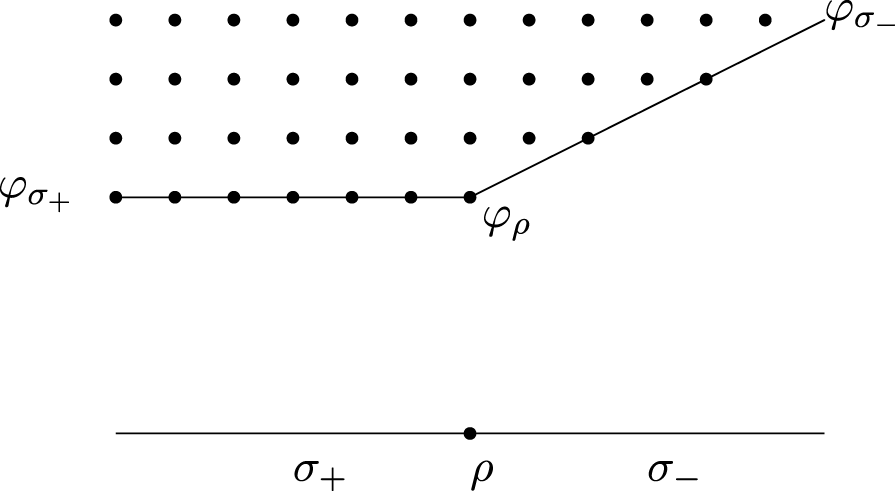
Figure 3. The monoid $P_{\unicode[STIX]{x1D711}_{\unicode[STIX]{x1D70C}}}$.

The monoids $P_{\unicode[STIX]{x1D711}_{\unicode[STIX]{x1D70E}_{+}}}$, $P_{\unicode[STIX]{x1D711}_{\unicode[STIX]{x1D70E}_{-}}}$ and $P_{\unicode[STIX]{x1D711}_{\unicode[STIX]{x1D70C}}}$ are represented in Figures 1–3.

For every $\unicode[STIX]{x1D70E}$ two-dimensional cone of $\unicode[STIX]{x1D6F4}$, we define $R_{\unicode[STIX]{x1D70E},I}^{\hbar }:=\unicode[STIX]{x1D55C}_{\hbar }[P_{\unicode[STIX]{x1D711}_{\unicode[STIX]{x1D70E}}}]/I$, a deformation quantization of $R_{\unicode[STIX]{x1D70E},I}:=\unicode[STIX]{x1D55C}[P_{\unicode[STIX]{x1D711}_{\unicode[STIX]{x1D70E}}}]/I$. We have a natural trivialization $P_{\unicode[STIX]{x1D711}_{\unicode[STIX]{x1D70E}}}=P\oplus \unicode[STIX]{x1D6EC}_{\unicode[STIX]{x1D70E}}$ and so $R_{\unicode[STIX]{x1D70E},I}^{\hbar }$ is simply the algebra of functions on a trivial family of two-dimensional quantum tori parametrized by $\operatorname{Spec}\,R_{I}$.

Let $\unicode[STIX]{x1D70C}$ be a one-dimensional cone of $\unicode[STIX]{x1D6F4}$. Let $\unicode[STIX]{x1D705}_{\unicode[STIX]{x1D70C},\unicode[STIX]{x1D711}}\in P$ be the kink of $\unicode[STIX]{x1D711}$ across $\unicode[STIX]{x1D70C}$, so that $z^{\unicode[STIX]{x1D705}_{\unicode[STIX]{x1D70C},\unicode[STIX]{x1D711}}}\in R_{I}$. Let $X$ be an invertible formal variable. We fix elements $\hat{f}_{\unicode[STIX]{x1D70C}^{\text{out}}}\in R_{I}^{\hbar }[X^{-1}]$ and $\hat{f}_{\unicode[STIX]{x1D70C}^{\text{in}}}\in R_{I}^{\hbar }[X]$.

Let $R_{\unicode[STIX]{x1D70C},I}^{\hbar }$ be the $R_{I}^{\hbar }$-algebra generated by formal variables $X_{+}$, $X_{-}$ and $X$, with $X$ invertible, and with relations

$$\begin{eqnarray}\displaystyle & XX_{+}=qX_{+}X, & \displaystyle \nonumber\\ \displaystyle & XX_{-}=q^{-1}X_{-}X, & \displaystyle \nonumber\\ \displaystyle & X_{+}X_{-}=q^{(1/2)D_{\unicode[STIX]{x1D70C}}^{2}}\hat{z}^{\unicode[STIX]{x1D705}_{\unicode[STIX]{x1D70C},\unicode[STIX]{x1D711}}}\hat{f}_{\unicode[STIX]{x1D70C}^{\text{out}}}(q^{-1}X)\hat{f}_{\unicode[STIX]{x1D70C}^{\text{in}}}(X)X^{-D_{\unicode[STIX]{x1D70C}}^{2}}, & \displaystyle \nonumber\\ \displaystyle & X_{-}X_{+}=q^{-(1/2)D_{\unicode[STIX]{x1D70C}}^{2}}\hat{z}^{\unicode[STIX]{x1D705}_{\unicode[STIX]{x1D70C},\unicode[STIX]{x1D711}}}\hat{f}_{\unicode[STIX]{x1D70C}^{\text{out}}}(X)\hat{f}_{\unicode[STIX]{x1D70C}^{\text{in}}}(qX)X^{-D_{\unicode[STIX]{x1D70C}}^{2}}, & \displaystyle \nonumber\end{eqnarray}$$

where $q=e^{i\hbar }$. The $R_{I}^{\hbar }$-algebra $R_{\unicode[STIX]{x1D70C},I}^{\hbar }$ is flat as $R_{I}^{\hbar }$-module and so is a deformation quantization of

$$\begin{eqnarray}R_{\unicode[STIX]{x1D70C},I}:=R_{I}[X_{+},X_{-},X^{\pm }]/(X_{+}X_{-}-z^{\unicode[STIX]{x1D705}_{\unicode[STIX]{x1D70C},\unicode[STIX]{x1D711}}}X^{-D_{\unicode[STIX]{x1D70C}}^{2}}f_{\unicode[STIX]{x1D70C}^{\text{out}}}(X)f_{\unicode[STIX]{x1D70C}^{\text{in}}}(X)).\end{eqnarray}$$

Let $\unicode[STIX]{x1D70E}_{+}$ and $\unicode[STIX]{x1D70E}_{-}$ be the two-dimensional cones of $\unicode[STIX]{x1D6F4}$ bounding $\unicode[STIX]{x1D70C}$, and let $\unicode[STIX]{x1D70C}_{+}$ and $\unicode[STIX]{x1D70C}_{-}$ be the other boundary rays of $\unicode[STIX]{x1D70E}_{+}$ and $\unicode[STIX]{x1D70E}_{-}$ respectively, such that $\unicode[STIX]{x1D70C}_{-}$, $\unicode[STIX]{x1D70C}$ and $\unicode[STIX]{x1D70C}_{+}$ are in anticlockwise order.

The precise form of $R_{\unicode[STIX]{x1D70C},I}^{\hbar }$ is justified by the following proposition.

Proposition 3.1. The map of $R_{I}^{\hbar }$-algebras

$$\begin{eqnarray}\tilde{\unicode[STIX]{x1D713}}_{\unicode[STIX]{x1D70C},-}:R_{I}^{\hbar }\langle X_{+},X_{-},X^{\pm }\rangle \rightarrow R_{\unicode[STIX]{x1D70E}_{-},I}^{\hbar }\end{eqnarray}$$

defined by

$$\begin{eqnarray}\displaystyle \tilde{\unicode[STIX]{x1D713}}_{\unicode[STIX]{x1D70C},-}(X) & = & \displaystyle \hat{z}^{\unicode[STIX]{x1D711}_{\unicode[STIX]{x1D70C}}(m_{\unicode[STIX]{x1D70C}})},\nonumber\\ \displaystyle \tilde{\unicode[STIX]{x1D713}}_{\unicode[STIX]{x1D70C},-}(X_{-}) & = & \displaystyle \hat{z}^{\unicode[STIX]{x1D711}_{\unicode[STIX]{x1D70C}}(m_{\unicode[STIX]{x1D70C}_{-}})},\nonumber\\ \displaystyle \tilde{\unicode[STIX]{x1D713}}_{\unicode[STIX]{x1D70C},-}(X_{+}) & = & \displaystyle \hat{f}_{\unicode[STIX]{x1D70C}^{\text{in}}}(\hat{z}^{\unicode[STIX]{x1D711}_{\unicode[STIX]{x1D70C}}(m_{\unicode[STIX]{x1D70C}})})\hat{z}^{\unicode[STIX]{x1D711}_{\unicode[STIX]{x1D70C}}(m_{\unicode[STIX]{x1D70C}_{+}})}\hat{f}_{\unicode[STIX]{x1D70C}^{\text{out}}}(\hat{z}^{\unicode[STIX]{x1D711}_{\unicode[STIX]{x1D70C}}(m_{\unicode[STIX]{x1D70C}})})\nonumber\\ \displaystyle & = & \displaystyle \hat{z}^{\unicode[STIX]{x1D711}_{\unicode[STIX]{x1D70C}}(m_{\unicode[STIX]{x1D70C}_{+}})}\hat{f}_{\unicode[STIX]{x1D70C}^{\text{in}}}(q\hat{z}^{\unicode[STIX]{x1D711}_{\unicode[STIX]{x1D70C}}(m_{\unicode[STIX]{x1D70C}})})\hat{f}_{\unicode[STIX]{x1D70C}^{\text{out}}}(\hat{z}^{\unicode[STIX]{x1D711}_{\unicode[STIX]{x1D70C}}(m_{\unicode[STIX]{x1D70C}})})\nonumber\end{eqnarray}$$

induces a map of $R_{I}^{\hbar }$-algebras

$$\begin{eqnarray}\hat{\unicode[STIX]{x1D713}}_{\unicode[STIX]{x1D70C},-}:R_{\unicode[STIX]{x1D70C},I}^{\hbar }\rightarrow R_{\unicode[STIX]{x1D70E}_{-},I}^{\hbar }.\end{eqnarray}$$

The map of $R_{I}^{\hbar }$-algebras

$$\begin{eqnarray}\tilde{\unicode[STIX]{x1D713}}_{\unicode[STIX]{x1D70C},+}:R_{I}^{\hbar }\langle X_{+},X_{-},X^{\pm }\rangle \rightarrow R_{\unicode[STIX]{x1D70E}_{+},I}^{\hbar }\end{eqnarray}$$

defined by

$$\begin{eqnarray}\displaystyle \tilde{\unicode[STIX]{x1D713}}_{\unicode[STIX]{x1D70C},+}(X) & = & \displaystyle \hat{z}^{\unicode[STIX]{x1D711}_{\unicode[STIX]{x1D70C}}(m_{\unicode[STIX]{x1D70C}})},\nonumber\\ \displaystyle \tilde{\unicode[STIX]{x1D713}}_{\unicode[STIX]{x1D70C},+}(X_{-}) & = & \displaystyle \hat{f}_{\unicode[STIX]{x1D70C}^{\text{out}}}(\hat{z}^{\unicode[STIX]{x1D711}_{\unicode[STIX]{x1D70C}}(m_{\unicode[STIX]{x1D70C}})})\hat{z}^{\unicode[STIX]{x1D711}_{\unicode[STIX]{x1D70C}}(m_{\unicode[STIX]{x1D70C}_{-}})}\hat{f}_{\unicode[STIX]{x1D70C}^{\text{in}}}(\hat{z}^{\unicode[STIX]{x1D711}_{\unicode[STIX]{x1D70C}}(m_{\unicode[STIX]{x1D70C}})})\nonumber\\ \displaystyle & = & \displaystyle \hat{z}^{\unicode[STIX]{x1D711}_{\unicode[STIX]{x1D70C}}(m_{\unicode[STIX]{x1D70C}_{-}})}\hat{f}_{\unicode[STIX]{x1D70C}^{\text{out}}}(q^{-1}\hat{z}^{\unicode[STIX]{x1D711}_{\unicode[STIX]{x1D70C}}(m_{\unicode[STIX]{x1D70C}})})\hat{f}_{\unicode[STIX]{x1D70C}^{\text{in}}}(\hat{z}^{\unicode[STIX]{x1D711}_{\unicode[STIX]{x1D70C}}(m_{\unicode[STIX]{x1D70C}})}),\nonumber\\ \displaystyle \tilde{\unicode[STIX]{x1D713}}_{\unicode[STIX]{x1D70C},+}(X_{+}) & = & \displaystyle \hat{z}^{\unicode[STIX]{x1D711}_{\unicode[STIX]{x1D70C}}(m_{\unicode[STIX]{x1D70C}_{+}})}\nonumber\end{eqnarray}$$

induces a map of $R_{I}^{\hbar }$-algebras

$$\begin{eqnarray}\hat{\unicode[STIX]{x1D713}}_{\unicode[STIX]{x1D70C},+}:R_{\unicode[STIX]{x1D70C},I}^{\hbar }\rightarrow R_{\unicode[STIX]{x1D70E}_{+},I}^{\hbar }.\end{eqnarray}$$

Proof. We have to check that $\tilde{\unicode[STIX]{x1D713}}_{\unicode[STIX]{x1D70C},-}$ and $\tilde{\unicode[STIX]{x1D713}}_{\unicode[STIX]{x1D70C},+}$ map the relations defining $R_{\unicode[STIX]{x1D70C},I}^{\hbar }$ to zero.

We have $\langle m_{\unicode[STIX]{x1D70C}},m_{\unicode[STIX]{x1D70C}_{+}}\rangle =1$ and $\langle m_{\unicode[STIX]{x1D70C}},m_{\unicode[STIX]{x1D70C}_{-}}\rangle =-1$. It follows that

$$\begin{eqnarray}\displaystyle \tilde{\unicode[STIX]{x1D713}}_{\unicode[STIX]{x1D70C},-}(XX_{+}-qX_{+}X) & = & \displaystyle 0,\nonumber\\ \displaystyle \tilde{\unicode[STIX]{x1D713}}_{\unicode[STIX]{x1D70C},+}(XX_{+}-qX_{+}X) & = & \displaystyle 0,\nonumber\end{eqnarray}$$

and

$$\begin{eqnarray}\displaystyle \tilde{\unicode[STIX]{x1D713}}_{\unicode[STIX]{x1D70C},-}(XX_{-}-q^{-1}X_{-}X) & = & \displaystyle 0,\nonumber\\ \displaystyle \tilde{\unicode[STIX]{x1D713}}_{\unicode[STIX]{x1D70C},+}(XX_{-}-q^{-1}X_{-}X) & = & \displaystyle 0.\nonumber\end{eqnarray}$$

Furthermore, we have

$$\begin{eqnarray}m_{\unicode[STIX]{x1D70C}_{-}}+D_{\unicode[STIX]{x1D70C}}^{2}m_{\unicode[STIX]{x1D70C}}+m_{\unicode[STIX]{x1D70C}_{+}}=0\end{eqnarray}$$

so

$$\begin{eqnarray}\langle m_{\unicode[STIX]{x1D70C}_{+}},m_{\unicode[STIX]{x1D70C}_{-}}\rangle =D_{\unicode[STIX]{x1D70C}}^{2}\end{eqnarray}$$

and

$$\begin{eqnarray}\unicode[STIX]{x1D711}_{\unicode[STIX]{x1D70C}}(m_{\unicode[STIX]{x1D70C}_{-}})+\unicode[STIX]{x1D711}_{\unicode[STIX]{x1D70C}}(m_{\unicode[STIX]{x1D70C}_{+}})=\unicode[STIX]{x1D705}_{\unicode[STIX]{x1D70C},\unicode[STIX]{x1D711}}-D_{\unicode[STIX]{x1D70C}}^{2}\unicode[STIX]{x1D711}_{\unicode[STIX]{x1D70C}}(m_{\unicode[STIX]{x1D70C}}).\end{eqnarray}$$

It follows that

$$\begin{eqnarray}\displaystyle \tilde{\unicode[STIX]{x1D713}}_{\unicode[STIX]{x1D70C},-}(X_{+}X_{-}) & = & \displaystyle \hat{f}_{\unicode[STIX]{x1D70C}^{\text{in}}}(\hat{z}^{\unicode[STIX]{x1D711}_{\unicode[STIX]{x1D70C}}(m_{\unicode[STIX]{x1D70C}})})\hat{z}^{\unicode[STIX]{x1D711}_{\unicode[STIX]{x1D70C}}(m_{\unicode[STIX]{x1D70C}_{+}})}\hat{f}_{\unicode[STIX]{x1D70C}^{\text{out}}}(\hat{z}^{\unicode[STIX]{x1D711}_{\unicode[STIX]{x1D70C}}(m_{\unicode[STIX]{x1D70C}})})\hat{z}^{\unicode[STIX]{x1D711}_{\unicode[STIX]{x1D70C}}(m_{\unicode[STIX]{x1D70C}_{-}})}\nonumber\\ \displaystyle & = & \displaystyle q^{(1/2)D_{\unicode[STIX]{x1D70C}}^{2}}\hat{f}_{\unicode[STIX]{x1D70C}^{\text{in}}}(\hat{z}^{\unicode[STIX]{x1D711}_{\unicode[STIX]{x1D70C}}(m_{\unicode[STIX]{x1D70C}})})\hat{f}_{\unicode[STIX]{x1D70C}^{\text{out}}}(q^{-1}\hat{z}^{\unicode[STIX]{x1D711}_{\unicode[STIX]{x1D70C}}(m_{\unicode[STIX]{x1D70C}})})\hat{z}^{\unicode[STIX]{x1D705}_{\unicode[STIX]{x1D70C},\unicode[STIX]{x1D711}}-D_{\unicode[STIX]{x1D70C}}^{2}\unicode[STIX]{x1D711}_{\unicode[STIX]{x1D70C}}(m_{\unicode[STIX]{x1D70C}})}\nonumber\\ \displaystyle & = & \displaystyle q^{(1/2)D_{\unicode[STIX]{x1D70C}}^{2}}\hat{z}^{\unicode[STIX]{x1D705}_{\unicode[STIX]{x1D70C},\unicode[STIX]{x1D711}}}\tilde{\unicode[STIX]{x1D713}}_{\unicode[STIX]{x1D70C},-}(\hat{f}_{\unicode[STIX]{x1D70C}^{\text{in}}}(X)\hat{f}_{\unicode[STIX]{x1D70C}^{\text{out}}}(q^{-1}X)X^{-D_{\unicode[STIX]{x1D70C}}^{2}}),\nonumber\\ \displaystyle \tilde{\unicode[STIX]{x1D713}}_{\unicode[STIX]{x1D70C},+}(X_{+}X_{-}) & = & \displaystyle \hat{z}^{\unicode[STIX]{x1D711}_{\unicode[STIX]{x1D70C}}(m_{\unicode[STIX]{x1D70C}_{+}})}\hat{f}_{\unicode[STIX]{x1D70C}^{\text{out}}}(\hat{z}^{\unicode[STIX]{x1D711}_{\unicode[STIX]{x1D70C}}(m_{\unicode[STIX]{x1D70C}})})\hat{z}^{\unicode[STIX]{x1D711}_{\unicode[STIX]{x1D70C}}(m_{\unicode[STIX]{x1D70C}_{-}})}\hat{f}_{\unicode[STIX]{x1D70C}^{\text{in}}}(\hat{z}^{\unicode[STIX]{x1D711}_{\unicode[STIX]{x1D70C}}(m_{\unicode[STIX]{x1D70C}})})\nonumber\\ \displaystyle & = & \displaystyle q^{(1/2)D_{\unicode[STIX]{x1D70C}}^{2}}\hat{f}_{\unicode[STIX]{x1D70C}^{\text{in}}}(\hat{z}^{\unicode[STIX]{x1D711}_{\unicode[STIX]{x1D70C}}(m_{\unicode[STIX]{x1D70C}})})\hat{f}_{\unicode[STIX]{x1D70C}^{\text{out}}}(q^{-1}\hat{z}^{\unicode[STIX]{x1D711}_{\unicode[STIX]{x1D70C}}(m_{\unicode[STIX]{x1D70C}})})\hat{z}^{\unicode[STIX]{x1D705}_{\unicode[STIX]{x1D70C},\unicode[STIX]{x1D711}}-D_{\unicode[STIX]{x1D70C}}^{2}\unicode[STIX]{x1D711}_{\unicode[STIX]{x1D70C}}(m_{\unicode[STIX]{x1D70C}})}\nonumber\\ \displaystyle & = & \displaystyle q^{(1/2)D_{\unicode[STIX]{x1D70C}}^{2}}\hat{z}^{\unicode[STIX]{x1D705}_{\unicode[STIX]{x1D70C},\unicode[STIX]{x1D711}}}\tilde{\unicode[STIX]{x1D713}}_{\unicode[STIX]{x1D70C},+}(\hat{f}_{\unicode[STIX]{x1D70C}^{\text{in}}}(X)\hat{f}_{\unicode[STIX]{x1D70C}^{\text{out}}}(q^{-1}X)X^{-D_{\unicode[STIX]{x1D70C}}^{2}}),\nonumber\end{eqnarray}$$

and

$$\begin{eqnarray}\displaystyle \tilde{\unicode[STIX]{x1D713}}_{\unicode[STIX]{x1D70C},-}(X_{-}X_{+}) & = & \displaystyle \hat{z}^{\unicode[STIX]{x1D711}_{\unicode[STIX]{x1D70C}}(m_{\unicode[STIX]{x1D70C}_{-}})}f_{\unicode[STIX]{x1D70C}^{\text{in}}}(\hat{z}^{\unicode[STIX]{x1D711}_{\unicode[STIX]{x1D70C}}(m_{\unicode[STIX]{x1D70C}})})\hat{z}^{\unicode[STIX]{x1D711}_{\unicode[STIX]{x1D70C}}(m_{\unicode[STIX]{x1D70C}_{+}})}f_{\unicode[STIX]{x1D70C}^{\text{out}}}(\hat{z}^{\unicode[STIX]{x1D711}_{\unicode[STIX]{x1D70C}}(m_{\unicode[STIX]{x1D70C}})})\nonumber\\ \displaystyle & = & \displaystyle q^{-(1/2)D_{\unicode[STIX]{x1D70C}}^{2}}\hat{z}^{\unicode[STIX]{x1D705}_{\unicode[STIX]{x1D70C},\unicode[STIX]{x1D711}}-D_{\unicode[STIX]{x1D70C}}^{2}\unicode[STIX]{x1D711}_{\unicode[STIX]{x1D70C}}(m_{\unicode[STIX]{x1D70C}})}f_{\unicode[STIX]{x1D70C}^{\text{in}}}(\hat{z}^{q\unicode[STIX]{x1D711}_{\unicode[STIX]{x1D70C}}(m_{\unicode[STIX]{x1D70C}})})f_{\unicode[STIX]{x1D70C}^{\text{out}}}(\hat{z}^{\unicode[STIX]{x1D711}_{\unicode[STIX]{x1D70C}}(m_{\unicode[STIX]{x1D70C}})})\nonumber\\ \displaystyle & = & \displaystyle q^{-(1/2)D_{\unicode[STIX]{x1D70C}}^{2}}\hat{z}^{\unicode[STIX]{x1D705}_{\unicode[STIX]{x1D70C},\unicode[STIX]{x1D711}}}\tilde{\unicode[STIX]{x1D713}}_{\unicode[STIX]{x1D70C},-}(\hat{f}_{\unicode[STIX]{x1D70C}^{\text{in}}}(qX)\hat{f}_{\unicode[STIX]{x1D70C}^{\text{out}}}(X)X^{-D_{\unicode[STIX]{x1D70C}}^{2}}),\nonumber\\ \displaystyle \tilde{\unicode[STIX]{x1D713}}_{\unicode[STIX]{x1D70C},+}(X_{-}X_{+}) & = & \displaystyle \hat{f}_{\unicode[STIX]{x1D70C}^{\text{out}}}(\hat{z}^{\unicode[STIX]{x1D711}_{\unicode[STIX]{x1D70C}}(m_{\unicode[STIX]{x1D70C}})})\hat{z}^{\unicode[STIX]{x1D711}_{\unicode[STIX]{x1D70C}}(m_{\unicode[STIX]{x1D70C}_{-}})}f_{\unicode[STIX]{x1D70C}^{\text{in}}}(\hat{z}^{\unicode[STIX]{x1D711}_{\unicode[STIX]{x1D70C}}(m_{\unicode[STIX]{x1D70C}})})\hat{z}^{\unicode[STIX]{x1D711}_{\unicode[STIX]{x1D70C}}(m_{\unicode[STIX]{x1D70C}_{+}})}\nonumber\\ \displaystyle & = & \displaystyle q^{-(1/2)D_{\unicode[STIX]{x1D70C}}^{2}}\hat{f}_{\unicode[STIX]{x1D70C}}(\hat{z}^{\unicode[STIX]{x1D711}_{\unicode[STIX]{x1D70C}}(m_{\unicode[STIX]{x1D70C}})})f_{\unicode[STIX]{x1D70C}^{\text{in}}}(q\hat{z}^{\unicode[STIX]{x1D711}_{\unicode[STIX]{x1D70C}}(m_{\unicode[STIX]{x1D70C}})})\hat{z}^{\unicode[STIX]{x1D705}_{\unicode[STIX]{x1D70C},\unicode[STIX]{x1D711}}-D_{\unicode[STIX]{x1D70C}}^{2}\unicode[STIX]{x1D711}_{\unicode[STIX]{x1D70C}}(m_{\unicode[STIX]{x1D70C}})}\nonumber\\ \displaystyle & = & \displaystyle q^{-(1/2)D_{\unicode[STIX]{x1D70C}}^{2}}\hat{z}^{\unicode[STIX]{x1D705}_{\unicode[STIX]{x1D70C},\unicode[STIX]{x1D711}}}\tilde{\unicode[STIX]{x1D713}}_{\unicode[STIX]{x1D70C},+}(\hat{f}_{\unicode[STIX]{x1D70C}^{\text{in}}}(qX)\hat{f}_{\unicode[STIX]{x1D70C}^{\text{out}}}(X)X^{-D_{\unicode[STIX]{x1D70C}}^{2}}).\Box \nonumber\end{eqnarray}$$

Remark.

1. – In the special case where $D_{\unicode[STIX]{x1D70C}}^{2}=0$ and $\hat{f}_{\unicode[STIX]{x1D70C}^{\text{in}}}=1$, our description of $R_{\unicode[STIX]{x1D70C},I}^{\hbar }$ by generators and relations coincides with the description given by Soibelman in [Reference SoibelmanSoi09, §7.5] of a local model for deformation quantization of a neighborhood of a focus–focus singularity.

2. – The algebra $R_{\unicode[STIX]{x1D70E},I}^{\hbar }$ is a deformation quantization of $R_{\unicode[STIX]{x1D70E},I}$, and $R_{\unicode[STIX]{x1D70C},I}^{\hbar }$ is a deformation quantization of $R_{\unicode[STIX]{x1D70C},I}$. The maps $\hat{\unicode[STIX]{x1D713}}_{\unicode[STIX]{x1D70C},+}$ and $\hat{\unicode[STIX]{x1D713}}_{\unicode[STIX]{x1D70C},-}$ are quantizations of the maps $\unicode[STIX]{x1D713}_{\unicode[STIX]{x1D70C},-}$ and $\unicode[STIX]{x1D713}_{\unicode[STIX]{x1D70C},+}$ defined by [Reference Gross, Hacking and KeelGHK15a, formula (2.8)]. Following [Reference Gross, Hacking and KeelGHK15a], we denote $U_{\unicode[STIX]{x1D70E},I}:=\operatorname{Spec}\,R_{\unicode[STIX]{x1D70E},I}$ and $U_{\unicode[STIX]{x1D70C},I}:=\operatorname{Spec}\,R_{\unicode[STIX]{x1D70C},I}$. If $\unicode[STIX]{x1D70C}$ is a one-dimensional cone of $\unicode[STIX]{x1D6F4}$, and $\unicode[STIX]{x1D70E}_{+}$ and $\unicode[STIX]{x1D70E}_{-}$ are the two-dimensional cones of $\unicode[STIX]{x1D6F4}$ bounding $\unicode[STIX]{x1D70C}$, then the maps $\unicode[STIX]{x1D713}_{\unicode[STIX]{x1D70C},-}$ and $\unicode[STIX]{x1D713}_{\unicode[STIX]{x1D70C},+}$ induce open immersions

   $$\begin{eqnarray}U_{\unicode[STIX]{x1D70E}-,I}{\hookrightarrow}U_{\unicode[STIX]{x1D70C},I}\end{eqnarray}$$
   and
   $$\begin{eqnarray}U_{\unicode[STIX]{x1D70E}+,I}{\hookrightarrow}U_{\unicode[STIX]{x1D70C},I}.\end{eqnarray}$$

Using Ore localization (see Definition 2.1), we can produce from $R_{\unicode[STIX]{x1D70E},I}^{\hbar }$ and $R_{\unicode[STIX]{x1D70C},I}^{\hbar }$ some sheaves of flat $\unicode[STIX]{x1D55C}_{\hbar }$-algebras ${\mathcal{O}}_{U_{\unicode[STIX]{x1D70E},I}}^{\hbar }$ and ${\mathcal{O}}_{U_{\unicode[STIX]{x1D70C},I}}^{\hbar }$ on $U_{\unicode[STIX]{x1D70E},I}$ and $U_{\unicode[STIX]{x1D70C},I}$, such that

$$\begin{eqnarray}{\mathcal{O}}_{U_{\unicode[STIX]{x1D70E},I}}^{\hbar }/\hbar {\mathcal{O}}_{U_{\unicode[STIX]{x1D70E},I}}^{\hbar }\simeq {\mathcal{O}}_{U_{\unicode[STIX]{x1D70E},I}}\end{eqnarray}$$

and

$$\begin{eqnarray}{\mathcal{O}}_{U_{\unicode[STIX]{x1D70C},I}}^{\hbar }/\hbar {\mathcal{O}}_{U_{\unicode[STIX]{x1D70C},I}}^{\hbar }\simeq {\mathcal{O}}_{U_{\unicode[STIX]{x1D70C},I}},\end{eqnarray}$$

respectively.

3.2 Quantum scattering diagrams

Quantum scattering diagrams have been studied by Filippini and Stoppa [Reference Filippini and StoppaFS15] in dimension two and by Mandel [Reference MandelMan15] in higher dimensions. Mandel [Reference MandelMan15] also studied quantum broken lines and quantum theta functions. Both [Reference Filippini and StoppaFS15] and [Reference MandelMan15] work with smooth integral affine manifolds. We need to make some changes to include the case we care about, where the integral affine manifold is the tropicalization $B$ of a Looijenga pair and has a singularity at the origin with a non-trivial monodromy around it.

As in the previous section, we fix a Looijenga pair $(Y,D)$, its tropicalization $(B,\unicode[STIX]{x1D6F4})$, a toric monoid $P$, a radical monomial ideal $J$ of $P$, and a $P_{\mathbb{R}}^{\text{gp}}$-valued multivalued convex $\unicode[STIX]{x1D6F4}$-piecewise linear $\unicode[STIX]{x1D711}$ function on $B$. Recall from §2.2 that we then have an exact sequence

$$\begin{eqnarray}0\rightarrow \text{}\underline{P}^{\text{gp}}\rightarrow {\mathcal{P}}\xrightarrow[{}]{\mathfrak{r}}\unicode[STIX]{x1D6EC}\rightarrow 0\,\end{eqnarray}$$

of locally constant sheaves on $B_{0}$.

We explained in §3.1 how to define, for every cone $\unicode[STIX]{x1D70F}$ of $\unicode[STIX]{x1D6F4}$, a toric monoid $P_{\unicode[STIX]{x1D711}_{\unicode[STIX]{x1D70F}}}$. We denote by

$$\begin{eqnarray}\unicode[STIX]{x1D55C}_{\hbar }\widehat{[P_{\unicode[STIX]{x1D711}_{\unicode[STIX]{x1D70F}}}]}\end{eqnarray}$$

the $J$-adic completion of the $\unicode[STIX]{x1D55C}_{\hbar }$-algebra $\unicode[STIX]{x1D55C}_{\hbar }[P_{\unicode[STIX]{x1D711}_{\unicode[STIX]{x1D70F}}}]$. The map $\mathfrak{r}:{\mathcal{P}}\rightarrow \unicode[STIX]{x1D6EC}$ induces a morphism of monoids $\mathfrak{r}:P_{\unicode[STIX]{x1D711}_{\unicode[STIX]{x1D70F}}}\rightarrow \unicode[STIX]{x1D6EC}_{\unicode[STIX]{x1D70F}}$.

Definition 3.1. A quantum scattering diagram $\hat{\mathfrak{D}}$ for the data $(B,\unicode[STIX]{x1D6F4})$, $P$, $J$ and $\unicode[STIX]{x1D711}$ is a set

$$\begin{eqnarray}\hat{\mathfrak{D}}=\{(\mathfrak{d},{\hat{H}}_{\mathfrak{d}})\},\end{eqnarray}$$

where $\mathfrak{d}\subset B$ is a ray of rational slope in $B$ with endpoint the origin $0\in B$.

1. – Let $\unicode[STIX]{x1D70F}_{\mathfrak{d}}$ be the smallest cone of $\unicode[STIX]{x1D6F4}$ containing $\mathfrak{d}$ and let $m_{\mathfrak{d}}\in \unicode[STIX]{x1D6EC}_{\unicode[STIX]{x1D70F}_{\mathfrak{d}}}$ be the primitive generator of $\mathfrak{d}$ pointing away from the origin. Then we have either

   $$\begin{eqnarray}{\hat{H}}_{\mathfrak{d}}=\mathop{\sum }_{\substack{ p\in P_{\unicode[STIX]{x1D711}_{\unicode[STIX]{x1D70F}_{\mathfrak{d}}}} \\ \mathfrak{r}(p)\in \mathbb{Z}_{{<}0}m_{\mathfrak{d}}}}H_{p}\hat{z}^{p}\in \unicode[STIX]{x1D55C}_{\hbar }\widehat{[P_{\unicode[STIX]{x1D711}_{\unicode[STIX]{x1D70F}_{\mathfrak{d}}}}]}\end{eqnarray}$$
   or
   $$\begin{eqnarray}{\hat{H}}_{\mathfrak{d}}=\mathop{\sum }_{\substack{ p\in P_{\unicode[STIX]{x1D711}_{\unicode[STIX]{x1D70F}_{\mathfrak{d}}}} \\ \mathfrak{r}(p)\in \mathbb{Z}_{{>}0}m_{\mathfrak{d}}}}H_{p}\hat{z}^{p}\in \unicode[STIX]{x1D55C}_{\hbar }\widehat{[P_{\unicode[STIX]{x1D711}_{\unicode[STIX]{x1D70F}_{\mathfrak{d}}}}]}.\end{eqnarray}$$
   In the first case, we say that the ray $(\mathfrak{d},{\hat{H}}_{\mathfrak{d}})$ is outgoing, and in the second case, we say that the ray $(\mathfrak{d},{\hat{H}}_{\mathfrak{d}})$ is ingoing.

2. – Let $\unicode[STIX]{x1D70F}_{\mathfrak{d}}$ be the smallest cone of $\unicode[STIX]{x1D6F4}$ containing $\mathfrak{d}$. If $\dim \unicode[STIX]{x1D70F}_{\mathfrak{d}}=2$, or if $\dim \unicode[STIX]{x1D70F}_{\mathfrak{d}}=1$ and $\unicode[STIX]{x1D705}_{\unicode[STIX]{x1D70F}_{\mathfrak{d}},\unicode[STIX]{x1D711}}\notin J$, then ${\hat{H}}_{\mathfrak{d}}=0\hspace{0.2em}{\rm mod}\hspace{0.2em}J$.

3. – For any ideal $I\subset P$ of radical $J$, there are only finitely many rays $(\mathfrak{d},{\hat{H}}_{\mathfrak{d}})$ such that ${\hat{H}}_{\mathfrak{d}}\neq 0\hspace{0.2em}{\rm mod}\hspace{0.2em}I$.

Given a ray $(\mathfrak{d},{\hat{H}}_{\mathfrak{d}})$ of a quantum scattering diagram, we call ${\hat{H}}_{\mathfrak{d}}$ the Hamiltonian attached to $\unicode[STIX]{x1D70C}$. This terminology is justified by §3.3, where we attach to $(\mathfrak{d},{\hat{H}}_{\mathfrak{d}})$ the automorphism $\hat{\unicode[STIX]{x1D6F7}}_{{\hat{H}}_{\mathfrak{d}}}$ given by the time-one evolution according to the quantum Hamiltonian ${\hat{H}}_{\mathfrak{d}}$.

3.3 Quantum automorphisms

Let $(\mathfrak{d},{\hat{H}}_{\mathfrak{d}})$ be a ray of a quantum scattering diagram $\hat{\mathfrak{D}}$ for the data $(B,\unicode[STIX]{x1D6F4})$, $P$, $J$ and $\unicode[STIX]{x1D711}$. Let $\unicode[STIX]{x1D70F}_{\mathfrak{d}}$ be the smallest cone of $\unicode[STIX]{x1D6F4}$ containing $\mathfrak{d}$ and let $m_{\mathfrak{d}}\in \unicode[STIX]{x1D6EC}_{\unicode[STIX]{x1D70F}_{\mathfrak{d}}}$ be the primitive generator of $\mathfrak{d}$ pointing away from the origin. Denote $m({\hat{H}}_{\mathfrak{d}})=m_{\mathfrak{d}}$ if $(\mathfrak{d},{\hat{H}}_{\mathfrak{d}})$ is outgoing and $m({\hat{H}}_{\mathfrak{d}})=-m_{\mathfrak{d}}$ if $(\mathfrak{d},{\hat{H}}_{\mathfrak{d}})$ is ingoing. Writing

$$\begin{eqnarray}{\hat{H}}_{\mathfrak{d}}=\mathop{\sum }_{p\in P_{\unicode[STIX]{x1D711}_{\unicode[STIX]{x1D70F}_{\mathfrak{d}}}}}H_{p}\hat{z}^{p}\in \unicode[STIX]{x1D55C}_{\hbar }\widehat{[P_{\unicode[STIX]{x1D711}_{\unicode[STIX]{x1D70F}_{\mathfrak{d}}}}]},\end{eqnarray}$$

we denote

$$\begin{eqnarray}\hat{f}_{\mathfrak{d}}:=\exp \biggl(\mathop{\sum }_{\substack{ p\in P_{\unicode[STIX]{x1D711}_{\unicode[STIX]{x1D70F}_{\mathfrak{d}}}} \\ \mathfrak{r}(p)=\ell m({\hat{H}}_{\mathfrak{d}})}}(q^{\ell }-1)H_{p}\hat{z}^{p}\biggr)\in \unicode[STIX]{x1D55C}_{\hbar }\widehat{[P_{\unicode[STIX]{x1D711}_{\unicode[STIX]{x1D70F}_{\mathfrak{d}}}}]},\end{eqnarray}$$

where $q=e^{i\hbar }$. Remark that, by our definition of $m({\hat{H}}_{\mathfrak{d}})$, we have $\ell \leqslant 0$ when writing $\mathfrak{r}(p)=\ell m({\hat{H}}_{\mathfrak{d}})$.

We write

$$\begin{eqnarray}\hat{f}_{\mathfrak{d}}=\mathop{\sum }_{p\in P_{\unicode[STIX]{x1D711}_{\unicode[STIX]{x1D70F}_{\mathfrak{d}}}}}f_{p}\hat{z}^{p}.\end{eqnarray}$$

For every $j\in \mathbb{Z}$, we define

$$\begin{eqnarray}\hat{f}_{\mathfrak{d}}(q^{j}\hat{z}):=\mathop{\sum }_{\substack{ p\in P_{\unicode[STIX]{x1D711}_{\unicode[STIX]{x1D70F}_{\mathfrak{d}}}} \\ \mathfrak{r}(p)=\ell m({\hat{H}}_{\mathfrak{d}})}}q^{\ell j}f_{p}\hat{z}^{p}\in \unicode[STIX]{x1D55C}_{\hbar }\widehat{[P_{\unicode[STIX]{x1D711}_{\unicode[STIX]{x1D70F}_{\mathfrak{d}}}}]},\end{eqnarray}$$

where $q=e^{i\hbar }$.

Lemma 3.1. The automorphism $\hat{\unicode[STIX]{x1D6F7}}_{{\hat{H}}_{\mathfrak{d}}}$ of $\unicode[STIX]{x1D55C}_{\hbar }\widehat{[P_{\unicode[STIX]{x1D711}_{\unicode[STIX]{x1D70F}_{\mathfrak{ d}}}}]}$ given by conjugation by $\exp ({\hat{H}}_{\mathfrak{d}})$,

$$\begin{eqnarray}\hat{z}^{p}\mapsto \exp ({\hat{H}}_{\mathfrak{ d}})\hat{z}^{p}\exp (-{\hat{H}}_{\mathfrak{ d}}),\end{eqnarray}$$

is equal to

$$\begin{eqnarray}\hat{z}^{p}\mapsto \left\{\begin{array}{@{}ll@{}}\displaystyle \hat{z}^{p}\mathop{\prod }_{j=0}^{\langle m({\hat{H}}_{\mathfrak{d}}),\mathfrak{r}(p)\rangle -1}\hat{f}_{\mathfrak{ d}}(q^{j}\hat{z})\quad & \text{if }\langle m({\hat{H}}_{\mathfrak{ d}}),\mathfrak{r}(p)\rangle \geqslant 0,\\ \displaystyle \hat{z}^{p}\mathop{\prod }_{j=0}^{|\langle m({\hat{H}}_{\mathfrak{d}}),\mathfrak{r}(p)\rangle |-1}\hat{f}_{\mathfrak{ d}}(q^{-j-1}\hat{z})^{-1}\quad & \text{if }\langle m({\hat{H}}_{\mathfrak{ d}}),\mathfrak{r}(p)\rangle <0.\end{array}\right.\end{eqnarray}$$

Proof. Using $\hat{z}^{p^{\prime }}\hat{z}^{p}=q^{\langle \mathfrak{r}(p^{\prime }),\mathfrak{r}(p)\rangle }\hat{z}^{p}\hat{z}^{p^{\prime }}$, we get

$$\begin{eqnarray}\exp ({\hat{H}}_{\mathfrak{d}})\hat{z}^{p}\exp (-{\hat{H}}_{\mathfrak{ d}})=\hat{z}^{p}\exp \biggl(\mathop{\sum }_{\substack{ p^{\prime }\in P_{\unicode[STIX]{x1D711}_{\unicode[STIX]{x1D70F}_{\mathfrak{d}}}} \\ \mathfrak{r}(p^{\prime })=\ell m({\hat{H}}_{\mathfrak{d}})}}(q^{\ell \langle m({\hat{H}}_{\mathfrak{d}}),\mathfrak{r}(p)\rangle }-1)H_{p^{\prime }}\hat{z}^{p^{\prime }}\biggr).\end{eqnarray}$$

If $\langle m({\hat{H}}_{\mathfrak{d}}),\mathfrak{r}(p)\rangle \geqslant 0$, this can be written

$$\begin{eqnarray}\displaystyle & & \displaystyle \hat{z}^{p}\exp \biggl(\mathop{\sum }_{\substack{ p^{\prime }\in P_{\unicode[STIX]{x1D711}_{\unicode[STIX]{x1D70F}_{\mathfrak{d}}}} \\ \mathfrak{r}(p^{\prime })=\ell m({\hat{H}}_{\mathfrak{d}})}}\frac{1-q^{\ell \langle m({\hat{H}}_{\mathfrak{d}}),\mathfrak{r}(p)\rangle }}{1-q^{\ell }}(q^{\ell }-1)H_{p^{\prime }}\hat{z}^{p^{\prime }}\biggr)\nonumber\\ \displaystyle & & \displaystyle \quad =\hat{z}^{p}\exp \biggl(\mathop{\sum }_{\substack{ p^{\prime }\in P_{\unicode[STIX]{x1D711}_{\unicode[STIX]{x1D70F}_{\mathfrak{d}}}} \\ \mathfrak{r}(p^{\prime })=\ell m({\hat{H}}_{\mathfrak{d}})}}\mathop{\sum }_{j=0}^{\langle m({\hat{H}}_{\mathfrak{d}}),\mathfrak{r}(p)\rangle -1}q^{\ell j}(q^{\ell }-1)H_{p^{\prime }}\hat{z}^{p^{\prime }}\biggr)\nonumber\\ \displaystyle & & \displaystyle \quad =\hat{z}^{p}\mathop{\prod }_{j=0}^{\langle m({\hat{H}}_{\mathfrak{d}}),\mathfrak{r}(p)\rangle -1}\hat{f}_{\mathfrak{ d}}(q^{j}\hat{z}).\nonumber\end{eqnarray}$$

If $\langle m({\hat{H}}_{\mathfrak{d}}),\mathfrak{r}(p)\rangle <0$, this can be written

$$\begin{eqnarray}\displaystyle & & \displaystyle \hat{z}^{p}\exp \biggl(-\mathop{\sum }_{\substack{ p^{\prime }\in P_{\unicode[STIX]{x1D711}_{\unicode[STIX]{x1D70F}_{\mathfrak{d}}}} \\ \mathfrak{r}(p^{\prime })=\ell m({\hat{H}}_{\mathfrak{d}})}}\frac{1-q^{-\ell |\langle m({\hat{H}}_{\mathfrak{d}}),\mathfrak{r}(p)\rangle |}}{1-q^{-\ell }}q^{-\ell }(q^{\ell }-1)H_{p^{\prime }}\hat{z}^{p^{\prime }}\biggr)\nonumber\\ \displaystyle & & \displaystyle \quad =\hat{z}^{p}\exp \biggl(-\mathop{\sum }_{\substack{ p^{\prime }\in P_{\unicode[STIX]{x1D711}_{\unicode[STIX]{x1D70F}_{\mathfrak{d}}}} \\ \mathfrak{r}(p^{\prime })=\ell m({\hat{H}}_{\mathfrak{d}})}}\mathop{\sum }_{j=0}^{|\langle m({\hat{H}}_{\mathfrak{d}}),\mathfrak{r}(p)\rangle |-1}(q^{-j-1})^{\ell }(q^{\ell }-1)H_{p^{\prime }}\hat{z}^{p^{\prime }}\biggr)\nonumber\\ \displaystyle & & \displaystyle \quad =\hat{z}^{p}\mathop{\prod }_{j=0}^{|\langle m({\hat{H}}_{\mathfrak{d}}),\mathfrak{r}(p)\rangle |-1}\hat{f}_{\mathfrak{ d}}(q^{-j-1}\hat{z})^{-1}.\Box \nonumber\end{eqnarray}$$

Remark.

One can equivalently write $\hat{\unicode[STIX]{x1D6F7}}_{{\hat{H}}_{\mathfrak{d}}}$ as

$$\begin{eqnarray}\hat{z}^{p}\mapsto \left\{\begin{array}{@{}ll@{}}\displaystyle \biggl(\mathop{\prod }_{j=0}^{\langle m({\hat{H}}_{\mathfrak{d}}),\mathfrak{r}(p)\rangle -1}\hat{f}_{\unicode[STIX]{x1D70C}}(q^{-j-1}z)\biggr)\hat{z}^{p}\quad & \text{if }\langle m({\hat{H}}_{\mathfrak{ d}}),\mathfrak{r}(p)\rangle \geqslant 0,\\ \displaystyle \biggl(\mathop{\prod }_{j=0}^{|\langle m({\hat{H}}_{\mathfrak{d}}),\mathfrak{r}(p)\rangle |-1}\hat{f}_{\unicode[STIX]{x1D70C}}(q^{j}z)^{-1}\biggr)\hat{z}^{p}\quad & \text{if }\langle m({\hat{H}}_{\mathfrak{ d}}),\mathfrak{r}(p)\rangle <0.\end{array}\right.\end{eqnarray}$$

A direct application of the definition of $\hat{f}_{\mathfrak{d}}$ gives the following lemma.

Lemma 3.2. If

$$\begin{eqnarray}{\hat{H}}=i\mathop{\sum }_{\ell \geqslant 1}\frac{(-1)^{\ell -1}}{\ell }\frac{\hat{z}^{-\ell \unicode[STIX]{x1D711}(m_{\mathfrak{d}})}}{2\sin (\ell \hbar /2)}=-\mathop{\sum }_{\ell \geqslant 1}\frac{(-1)^{\ell -1}}{\ell }\frac{\hat{z}^{-\ell \unicode[STIX]{x1D711}(m_{\mathfrak{d}})}}{q^{\ell /2}-q^{-\ell /2}},\end{eqnarray}$$

where $q=e^{i\hbar }$, we have $m({\hat{H}})=m_{\mathfrak{d}}$ and

$$\begin{eqnarray}\hat{f}=\exp \biggl(-\mathop{\sum }_{\ell \geqslant 1}\frac{(-1)^{\ell -1}}{\ell }\frac{q^{-\ell }-1}{q^{\ell /2}-q^{-\ell /2}}\hat{z}^{-\ell \unicode[STIX]{x1D711}(m_{\mathfrak{d}})}\biggr)=1+q^{-1/2}\hat{z}^{-\unicode[STIX]{x1D711}(m_{\mathfrak{d}})}.\end{eqnarray}$$

If

$$\begin{eqnarray}{\hat{H}}=i\mathop{\sum }_{\ell \geqslant 1}\frac{(-1)^{\ell -1}}{\ell }\frac{\hat{z}^{\ell \unicode[STIX]{x1D711}(m_{\mathfrak{d}})}}{2\sin (\ell \hbar /2)}=-\mathop{\sum }_{\ell \geqslant 1}\frac{(-1)^{\ell -1}}{\ell }\frac{\hat{z}^{\ell \unicode[STIX]{x1D711}(m_{\mathfrak{d}})}}{q^{\ell /2}-q^{-\ell /2}},\end{eqnarray}$$

where $q=e^{i\hbar }$, we have $m({\hat{H}})=-m_{\mathfrak{d}}$ and

$$\begin{eqnarray}\hat{f}=\exp \biggl(-\mathop{\sum }_{\ell \geqslant 1}\frac{(-1)^{\ell -1}}{\ell }\frac{q^{-\ell }-1}{q^{\ell /2}-q^{-\ell /2}}\hat{z}^{\ell \unicode[STIX]{x1D711}(m_{\mathfrak{d}})}\biggr)=1+q^{-1/2}\hat{z}^{\unicode[STIX]{x1D711}(m_{\mathfrak{d}})}.\end{eqnarray}$$

3.4 Gluing

We fix a quantum scattering diagram $\hat{\mathfrak{D}}$ for the data $(B,\unicode[STIX]{x1D6F4})$, $P$, $J$ and $\unicode[STIX]{x1D711}$, and an ideal $I$ of radical $J$.

Let $\unicode[STIX]{x1D70C}$ be a one-dimensional cone of $\unicode[STIX]{x1D6F4}$, bounding the two-dimensional cones $\unicode[STIX]{x1D70E}_{+}$ and $\unicode[STIX]{x1D70E}_{-}$, such that $\unicode[STIX]{x1D70E}_{-}$, $\unicode[STIX]{x1D70C}$, $\unicode[STIX]{x1D70E}_{+}$ are in anticlockwise order. Identifying $X$ with $\hat{z}^{\unicode[STIX]{x1D711}_{\unicode[STIX]{x1D70C}}(m_{\unicode[STIX]{x1D70C}})}$, we define $\hat{f}_{\unicode[STIX]{x1D70C}^{\text{out}}}\in R_{I}^{\hbar }[X^{-1}]$ by

$$\begin{eqnarray}\hat{f}_{\unicode[STIX]{x1D70C}^{\text{out}}}:=\mathop{\prod }_{\substack{ \mathfrak{d}\in \hat{\mathfrak{D}},\mathfrak{d}=\unicode[STIX]{x1D70C} \\ \text{outgoing}}}\hat{f}_{\mathfrak{d}}\hspace{0.2em}{\rm mod}\hspace{0.2em}I,\end{eqnarray}$$

where the product is over the outgoing rays of $\hat{\mathfrak{D}}$ of support $\unicode[STIX]{x1D70C}$, and we define $\hat{f}_{\unicode[STIX]{x1D70C}^{\text{in}}}\in R_{I}^{\hbar }[X]$ by

$$\begin{eqnarray}\hat{f}_{\unicode[STIX]{x1D70C}^{\text{in}}}:=\mathop{\prod }_{\substack{ \mathfrak{d}\in \hat{\mathfrak{D}},\mathfrak{d}=\unicode[STIX]{x1D70C} \\ \text{ingoing}}}\hat{f}_{\mathfrak{d}}\hspace{0.2em}{\rm mod}\hspace{0.2em}I,\end{eqnarray}$$

where the product is over the ingoing rays of $\hat{\mathfrak{D}}$ of support $\unicode[STIX]{x1D70C}$.

By §3.1, we then have $R_{I}^{\hbar }$-algebras $R_{\unicode[STIX]{x1D70E}_{+},I}^{\hbar }$, $R_{\unicode[STIX]{x1D70E}_{-},I}^{\hbar }$, $R_{\unicode[STIX]{x1D70C},I}^{\hbar }$.

Let $(\mathfrak{d},{\hat{H}}_{\mathfrak{d}})$ be a ray of $\hat{\mathfrak{D}}$ such that $\unicode[STIX]{x1D70F}_{\mathfrak{d}}=\unicode[STIX]{x1D70E}$ is a two-dimensional cone of $\unicode[STIX]{x1D6F4}$. Let $m_{\mathfrak{d}}\in \unicode[STIX]{x1D6EC}_{\unicode[STIX]{x1D70F}_{\mathfrak{d}}}$ be the primitive generator of $\mathfrak{d}$ pointing away from the origin. Let $\unicode[STIX]{x1D6FE}$ be a path in $B_{0}$ which crosses $\mathfrak{d}$ transversally at time $t_{0}$. We define

$$\begin{eqnarray}\displaystyle & \hat{\unicode[STIX]{x1D703}}_{\unicode[STIX]{x1D6FE},\mathfrak{d}}:R_{\unicode[STIX]{x1D70E},I}^{\hbar }\rightarrow R_{\unicode[STIX]{x1D70E},I}^{\hbar }, & \displaystyle \nonumber\\ \displaystyle & \hat{z}^{p}\mapsto \hat{\unicode[STIX]{x1D6F7}}_{{\hat{H}}_{\mathfrak{d}}}^{\unicode[STIX]{x1D716}}(\hat{z}^{p}), & \displaystyle \nonumber\end{eqnarray}$$

where $\unicode[STIX]{x1D716}\in \{\pm 1\}$ is the sign of $-\langle m({\hat{H}}_{\mathfrak{d}}),\unicode[STIX]{x1D6FE}^{\prime }(t_{0})\rangle$.

Let $\hat{\mathfrak{D}}_{I}\subset \hat{\mathfrak{D}}$ be the finite set of rays $(\mathfrak{d},{\hat{H}}_{\mathfrak{d}})$ with ${\hat{H}}_{\mathfrak{d}}\neq 0\hspace{0.2em}{\rm mod}\hspace{0.2em}I$, that is, $\hat{f}_{\mathfrak{d}}\neq 1\hspace{0.2em}{\rm mod}\hspace{0.2em}I$. If $\unicode[STIX]{x1D6FE}$ is a path in $B_{0}$ entirely contained in the interior of a two-dimensional cone $\unicode[STIX]{x1D70E}$ of $\unicode[STIX]{x1D6F4}$, and crossing elements of $\mathfrak{D}_{I}$ transversally, we define

$$\begin{eqnarray}\hat{\unicode[STIX]{x1D703}}_{\unicode[STIX]{x1D6FE},\hat{\mathfrak{D}}_{I}}:=\hat{\unicode[STIX]{x1D703}}_{\unicode[STIX]{x1D6FE},\mathfrak{d}_{n}}\circ \ldots \circ \hat{\unicode[STIX]{x1D703}}_{\unicode[STIX]{x1D6FE},\mathfrak{d}_{1}},\end{eqnarray}$$

where $\unicode[STIX]{x1D6FE}$ crosses the elements $\mathfrak{d}_{1},\ldots ,\mathfrak{d}_{n}$ of $\hat{\mathfrak{D}}_{I}$ in the given order.

For every $\unicode[STIX]{x1D70E}$ two-dimensional cone of $\unicode[STIX]{x1D6F4}$, bounded by rays $\unicode[STIX]{x1D70C}_{R}$ and $\unicode[STIX]{x1D70C}_{L}$, such that $\unicode[STIX]{x1D70C}_{R},\unicode[STIX]{x1D70E},\unicode[STIX]{x1D70C}_{L}$ are in anticlockwise order, we choose a path $\unicode[STIX]{x1D6FE}_{\unicode[STIX]{x1D70E}}:[0,1]\rightarrow B_{0}$ whose image is entirely contained in the interior of $\unicode[STIX]{x1D70E}$, with $\unicode[STIX]{x1D6FE}(0)$ close to $\unicode[STIX]{x1D70C}_{R}$ and $\unicode[STIX]{x1D6FE}(1)$ close to $\unicode[STIX]{x1D70C}_{L}$, such that $\unicode[STIX]{x1D6FE}_{\unicode[STIX]{x1D70E}}$ crosses every ray of $\hat{\mathfrak{D}}_{I}$ contained in $\unicode[STIX]{x1D70E}$ transversally exactly once. Let

$$\begin{eqnarray}\hat{\unicode[STIX]{x1D703}}_{\unicode[STIX]{x1D6FE}_{\unicode[STIX]{x1D70E}},\hat{\mathfrak{D}}_{I}}:R_{\unicode[STIX]{x1D70E},I}^{\hbar }\rightarrow R_{\unicode[STIX]{x1D70E},I}^{\hbar }\end{eqnarray}$$

be the corresponding automorphism. In the classical limit, $\hat{\unicode[STIX]{x1D703}}_{\unicode[STIX]{x1D6FE},\hat{\mathfrak{D}}_{I}}$ induces an automorphism $\unicode[STIX]{x1D703}_{\unicode[STIX]{x1D6FE},\mathfrak{D}_{I}}$ of $U_{\unicode[STIX]{x1D70E},I}$. Gluing together the open sets $U_{\unicode[STIX]{x1D70E},I}\subset U_{\unicode[STIX]{x1D70C}_{R},I}$ and $U_{\unicode[STIX]{x1D70E},I}\subset U_{\unicode[STIX]{x1D70C}_{L},I}$ along these automorphisms, we get the scheme $X_{I,\mathfrak{D}}^{\circ }$ defined in [Reference Gross, Hacking and KeelGHK15a].

Recall from the end of §3.1 that by Ore localization the algebras $R_{\unicode[STIX]{x1D70E},I}^{\hbar }$ and $R_{\unicode[STIX]{x1D70C},I}^{\hbar }$ produce sheaves ${\mathcal{O}}_{U_{\unicode[STIX]{x1D70E},I}}^{\hbar }$ and ${\mathcal{O}}_{U_{\unicode[STIX]{x1D70C},I}}^{\hbar }$ on $U_{\unicode[STIX]{x1D70E},I}$ and $U_{\unicode[STIX]{x1D70C},I}$, respectively. Using $\hat{\unicode[STIX]{x1D703}}_{\unicode[STIX]{x1D6FE}_{\unicode[STIX]{x1D70E}},\hat{\mathfrak{D}}_{I}}$, we can glue together the sheaves ${\mathcal{O}}_{U_{\unicode[STIX]{x1D70C},I}}^{\hbar }$ to get a sheaf of $R_{I}^{\hbar }$-algebras ${\mathcal{O}}_{X_{I,\mathfrak{D}}^{\circ }}^{\hbar }$ on $X_{I,\mathfrak{D}}^{\circ }$.

From the fact that the sheaves ${\mathcal{O}}_{U_{\unicode[STIX]{x1D70C},I}}^{\hbar }$ are deformation quantizations of $U_{\unicode[STIX]{x1D70C},I}$, we deduce that the sheaf ${\mathcal{O}}_{X_{I,\mathfrak{D}}^{\circ }}^{\hbar }$ is a deformation quantization of $X_{I,\mathfrak{D}}^{\circ }$. In particular, we have ${\mathcal{O}}_{X_{I,\mathfrak{D}}^{\circ }}^{\hbar }/\hbar {\mathcal{O}}_{X_{I,\mathfrak{D}}^{\circ }}^{\hbar }={\mathcal{O}}_{X_{I,\mathfrak{D}}^{\circ }}$ and ${\mathcal{O}}_{X_{I,\mathfrak{D}}^{\circ }}^{\hbar }$ is a sheaf a flat $R_{I}^{\hbar }$-algebras.

Remark.

Let $\unicode[STIX]{x1D70C}$ be a one-dimensional cone of $\unicode[STIX]{x1D6F4}$. Let $\unicode[STIX]{x1D70E}_{+}$ and $\unicode[STIX]{x1D70E}_{-}$ be the two two-dimensional cones of $\unicode[STIX]{x1D6F4}$ bounding $\unicode[STIX]{x1D70C}$, and let $\unicode[STIX]{x1D70C}_{+}$ and $\unicode[STIX]{x1D70C}_{-}$ be the other boundary rays of $\unicode[STIX]{x1D70E}_{+}$ and $\unicode[STIX]{x1D70E}_{-}$ respectively, such that $\unicode[STIX]{x1D70C}_{-}$, $\unicode[STIX]{x1D70C}$ and $\unicode[STIX]{x1D70C}_{+}$ are in anticlockwise order. According to [Reference Gross, Hacking and KeelGHK15a, Remark 2.6], we have, in $U_{\unicode[STIX]{x1D70C},I}$,

$$\begin{eqnarray}U_{\unicode[STIX]{x1D70C}_{-},I}\cap U_{\unicode[STIX]{x1D70C}_{+},I}\simeq (\mathbb{G}_{m})^{2}\times \operatorname{Spec}\,(R_{I})_{z^{\unicode[STIX]{x1D705}_{\unicode[STIX]{x1D70C},\unicode[STIX]{x1D711}}}},\end{eqnarray}$$

where $(R_{I})_{z^{\unicode[STIX]{x1D705}_{\unicode[STIX]{x1D70C},\unicode[STIX]{x1D711}}}}$ is the localization of $R_{I}$ defined by inverting $z^{\unicode[STIX]{x1D705}_{\unicode[STIX]{x1D70C},\unicode[STIX]{x1D711}}}$. Similarly, the restriction of ${\mathcal{O}}_{X_{I,\mathfrak{D}}^{\circ }}^{\hbar }$ to $U_{\unicode[STIX]{x1D70C}_{-},I}\cap U_{\unicode[STIX]{x1D70C}_{+},I}$ is the Ore localization of $\unicode[STIX]{x1D55C}_{\hbar }[M]\,\hat{\otimes }\,(R_{I})_{z^{\unicode[STIX]{x1D705}_{\unicode[STIX]{x1D70C},\unicode[STIX]{x1D711}}}}$, where $M=\mathbb{Z}^{2}$ is the character lattice of $(\mathbb{G}_{m})^{2}$, equipped with the standard unimodular integral symplectic pairing. We have a natural identification $M=\unicode[STIX]{x1D6EC}_{\unicode[STIX]{x1D70C}}$. Restricted to $\unicode[STIX]{x1D55C}_{\hbar }[M]\,\hat{\otimes }\,(R_{I})_{z^{\unicode[STIX]{x1D705}_{\unicode[STIX]{x1D70C},\unicode[STIX]{x1D711}}}}$, and assuming that $\hat{f}_{\unicode[STIX]{x1D70C}^{\text{in}}}=1\hspace{0.2em}{\rm mod}\hspace{0.2em}\hat{z}^{\unicode[STIX]{x1D705}_{\unicode[STIX]{x1D70C},\unicode[STIX]{x1D711}}}$ and $\hat{f}_{\unicode[STIX]{x1D70C}^{\text{out}}}=1\hspace{0.2em}{\rm mod}\hspace{0.2em}\hat{z}^{\unicode[STIX]{x1D705}_{\unicode[STIX]{x1D70C},\unicode[STIX]{x1D711}}}$, the expression $\hat{\unicode[STIX]{x1D713}}_{\unicode[STIX]{x1D70C}_{+}}\circ \hat{\unicode[STIX]{x1D713}}_{\unicode[STIX]{x1D70C}_{-}}^{-1}$ makes senseFootnote ¹⁰ and is given by

$$\begin{eqnarray}\displaystyle (\hat{\unicode[STIX]{x1D713}}_{\unicode[STIX]{x1D70C}_{+}}\circ \hat{\unicode[STIX]{x1D713}}_{\unicode[STIX]{x1D70C}_{-}}^{-1})(\hat{z}^{\unicode[STIX]{x1D711}_{\unicode[STIX]{x1D70C}}(m_{\unicode[STIX]{x1D70C}})}) & = & \displaystyle \hat{z}^{\unicode[STIX]{x1D711}_{\unicode[STIX]{x1D70C}}(m_{\unicode[STIX]{x1D70C}})},\nonumber\\ \displaystyle (\hat{\unicode[STIX]{x1D713}}_{\unicode[STIX]{x1D70C}_{+}}\circ \hat{\unicode[STIX]{x1D713}}_{\unicode[STIX]{x1D70C}_{-}}^{-1})(\hat{z}^{\unicode[STIX]{x1D711}_{\unicode[STIX]{x1D70C}}(m_{\unicode[STIX]{x1D70C}_{-}})}) & = & \displaystyle \hat{f}_{\unicode[STIX]{x1D70C}^{\text{out}}}(\hat{z}^{\unicode[STIX]{x1D711}_{\unicode[STIX]{x1D70C}}(m_{\unicode[STIX]{x1D70C}})})\hat{z}^{\unicode[STIX]{x1D711}_{\unicode[STIX]{x1D70C}}(m_{\unicode[STIX]{x1D70C}_{-}})}\hat{f}_{\unicode[STIX]{x1D70C}^{\text{in}}}(\hat{z}^{\unicode[STIX]{x1D711}_{\unicode[STIX]{x1D70C}}(m_{\unicode[STIX]{x1D70C}})}),\nonumber\\ \displaystyle (\hat{\unicode[STIX]{x1D713}}_{\unicode[STIX]{x1D70C}_{+}}\circ \hat{\unicode[STIX]{x1D713}}_{\unicode[STIX]{x1D70C}_{-}}^{-1})(\hat{z}^{\unicode[STIX]{x1D711}_{\unicode[STIX]{x1D70C}}(m_{\unicode[STIX]{x1D70C}_{+}})}) & = & \displaystyle \hat{f}_{\unicode[STIX]{x1D70C}^{\text{in}}}^{-1}(\hat{z}^{\unicode[STIX]{x1D711}_{\unicode[STIX]{x1D70C}}(m_{\unicode[STIX]{x1D70C}})})\hat{z}^{\unicode[STIX]{x1D711}_{\unicode[STIX]{x1D70C}}(m_{\unicode[STIX]{x1D70C}_{+}})}\hat{f}_{\unicode[STIX]{x1D70C}^{\text{out}}}^{-1}(\hat{z}^{\unicode[STIX]{x1D711}_{\unicode[STIX]{x1D70C}}(m_{\unicode[STIX]{x1D70C}})}).\nonumber\end{eqnarray}$$

As $\langle m_{\unicode[STIX]{x1D70C}},m_{\unicode[STIX]{x1D70C}_{-}}\rangle =-1$ and $\langle m_{\unicode[STIX]{x1D70C}},m_{\unicode[STIX]{x1D70C}_{+}}\rangle =1$, this implies that $\hat{\unicode[STIX]{x1D713}}_{\unicode[STIX]{x1D70C}_{+}}\circ \hat{\unicode[STIX]{x1D713}}_{\unicode[STIX]{x1D70C}_{-}}^{-1}$ coincides with the transformation

$$\begin{eqnarray}\hat{\unicode[STIX]{x1D703}}_{\unicode[STIX]{x1D6FE},\unicode[STIX]{x1D70C}}=\mathop{\prod }_{\mathfrak{d}\in \mathfrak{D},\mathfrak{d}=\unicode[STIX]{x1D70C}}\hat{\unicode[STIX]{x1D703}}_{\unicode[STIX]{x1D6FE},\mathfrak{d}},\end{eqnarray}$$

where $\hat{\unicode[STIX]{x1D703}}_{\unicode[STIX]{x1D6FE},\mathfrak{d}}$ is defined by the same formulas as above and with $\unicode[STIX]{x1D6FE}$ a path intersecting $\unicode[STIX]{x1D70C}$ at a single point and going from $\unicode[STIX]{x1D70E}_{-}$ to $\unicode[STIX]{x1D70E}_{+}$.

3.5 Result of the gluing for $I=J$

Assume $r\geqslant 3$ and $\unicode[STIX]{x1D705}_{\unicode[STIX]{x1D70C},\unicode[STIX]{x1D711}}\in J$ for every $\unicode[STIX]{x1D70C}$ one-dimensional cone of $\unicode[STIX]{x1D6F4}$. Lemma 3.3 below gives an explicit description of ${\mathcal{O}}_{X_{I,\mathfrak{D}}^{\circ }}^{\hbar }$ for $I=J$.

Denote by $\unicode[STIX]{x1D55C}[\unicode[STIX]{x1D6F4}]$ the $\unicode[STIX]{x1D55C}$-algebra with a $\unicode[STIX]{x1D55C}$-basis $\{z^{m}\mid m\in B(\mathbb{Z})\}$ with multiplication given by

Let $0$ be the closed point of $\operatorname{Spec}\,\unicode[STIX]{x1D55C}[\unicode[STIX]{x1D6F4}]$ whose ideal is generated by $\{z^{m}\mid m\neq 0\}$. Denote $R_{J}[\unicode[STIX]{x1D6F4}]:=R_{J}\otimes _{\unicode[STIX]{x1D55C}}\unicode[STIX]{x1D55C}[\unicode[STIX]{x1D6F4}]$. According to [Reference Gross, Hacking and KeelGHK15a, Lemma 2.12], we have

$$\begin{eqnarray}X_{J}^{\circ }\simeq (\operatorname{Spec}\,R_{J}[\unicode[STIX]{x1D6F4}])-((\operatorname{Spec}\,R_{J})\times \{0\}).\end{eqnarray}$$

Denote by $\unicode[STIX]{x1D55C}_{\hbar }[\unicode[STIX]{x1D6F4}]$ the $\unicode[STIX]{x1D55C}_{\hbar }$-algebra with a $\unicode[STIX]{x1D55C}_{\hbar }$-basis $\{\hat{z}^{m}\mid m\in B(\mathbb{Z})\}$ with multiplication given by

Denote $R_{J}^{\hbar }[\unicode[STIX]{x1D6F4}]:=R_{J}\,\hat{\otimes }_{\unicode[STIX]{x1D55C}}\,\unicode[STIX]{x1D55C}_{\hbar }[\unicode[STIX]{x1D6F4}]$.

Proof. By definition of a quantum scattering diagram, if $\mathfrak{d}$ is contained in the interior of a two-dimensional cone of $\unicode[STIX]{x1D6F4}$, we have ${\hat{H}}_{\mathfrak{d}}=0\hspace{0.2em}{\rm mod}\hspace{0.2em}J$ and so the corresponding automorphism $\hat{\unicode[STIX]{x1D6F7}}_{{\hat{H}}_{\mathfrak{d}}}$ is the identity. As we are assuming $\unicode[STIX]{x1D705}_{\unicode[STIX]{x1D70C},\unicode[STIX]{x1D711}}\in J$, $R_{\unicode[STIX]{x1D70C},J}^{\hbar }$ is the $R_{J}^{\hbar }$-algebra generated by formal variables $X_{+}$, $X_{-}$ and $X$, with $X$ invertible, and with relations

$$\begin{eqnarray}\displaystyle XX_{+} & = & \displaystyle qXX_{+},\nonumber\\ \displaystyle XX_{-} & = & \displaystyle q^{-1}X_{-}X,\nonumber\\ \displaystyle X_{+}X_{-} & = & \displaystyle X_{-}X_{+}=0,\nonumber\end{eqnarray}$$

where $q=e^{i\hbar }$. Let $\unicode[STIX]{x1D70E}_{+}$ and $\unicode[STIX]{x1D70E}_{-}$ be the two two-dimensional cones of $\unicode[STIX]{x1D6F4}$ bounding $\unicode[STIX]{x1D70C}$, and let $\unicode[STIX]{x1D70C}_{+}$ and $\unicode[STIX]{x1D70C}_{-}$ be the other boundary rays of $\unicode[STIX]{x1D70E}_{+}$ and $\unicode[STIX]{x1D70E}_{-}$ respectively, such that $\unicode[STIX]{x1D70C}_{-}$, $\unicode[STIX]{x1D70C}$ and $\unicode[STIX]{x1D70C}_{+}$ are in anticlockwise order.

From $\unicode[STIX]{x1D711}_{\unicode[STIX]{x1D70C}}(m_{\unicode[STIX]{x1D70C}_{-}})+\unicode[STIX]{x1D711}_{\unicode[STIX]{x1D70C}}(m_{\unicode[STIX]{x1D70C}_{+}})=\unicode[STIX]{x1D705}_{\unicode[STIX]{x1D70C},\unicode[STIX]{x1D711}}-D_{\unicode[STIX]{x1D70C}}^{2}\unicode[STIX]{x1D711}_{\unicode[STIX]{x1D70C}}(m_{\unicode[STIX]{x1D70C}})$ and $\unicode[STIX]{x1D705}_{\unicode[STIX]{x1D70C},\unicode[STIX]{x1D711}}\in J$, we deduce that $\hat{z}^{\unicode[STIX]{x1D711}_{\unicode[STIX]{x1D70C}}(m_{\unicode[STIX]{x1D70C}_{-}})}\hat{z}^{\unicode[STIX]{x1D711}_{\unicode[STIX]{x1D70C}}(m_{\unicode[STIX]{x1D70C}_{+}})}=0$ in $R_{\unicode[STIX]{x1D70C},I}^{\hbar }$, $R_{\unicode[STIX]{x1D70E}_{-}I}^{\hbar }$ and $R_{\unicode[STIX]{x1D70E}_{+},I}^{\hbar }$. As $\hat{z}^{\unicode[STIX]{x1D711}_{\unicode[STIX]{x1D70C}}(m_{\unicode[STIX]{x1D70C}_{-}})}$ is invertible in $R_{\unicode[STIX]{x1D70E}_{-}I}^{\hbar }$, we have $\hat{z}^{\unicode[STIX]{x1D711}_{\unicode[STIX]{x1D70C}}(m_{\unicode[STIX]{x1D70C}_{+}})}=0$ in $R_{\unicode[STIX]{x1D70E}_{-}I}^{\hbar }$. Similarly, as $\hat{z}^{\unicode[STIX]{x1D711}_{\unicode[STIX]{x1D70C}}(m_{\unicode[STIX]{x1D70C}_{+}})}$ is invertible in $R_{\unicode[STIX]{x1D70E}_{+}I}^{\hbar }$, we have $\hat{z}^{\unicode[STIX]{x1D711}_{\unicode[STIX]{x1D70C}}(m_{\unicode[STIX]{x1D70C}_{-}})}=0$ in $R_{\unicode[STIX]{x1D70E}_{+}I}^{\hbar }$.

So the map $\hat{\unicode[STIX]{x1D713}}_{\unicode[STIX]{x1D70C},-}:R_{\unicode[STIX]{x1D70C},J}^{\hbar }\rightarrow R_{\unicode[STIX]{x1D70E}_{-},J}^{\hbar }$ is given by $\hat{\unicode[STIX]{x1D713}}_{\unicode[STIX]{x1D70C},-}(X)=\hat{z}^{\unicode[STIX]{x1D711}_{\unicode[STIX]{x1D70C}}(m_{\unicode[STIX]{x1D70C}})}$, $\hat{\unicode[STIX]{x1D713}}_{\unicode[STIX]{x1D70C},-}(X_{-})=\hat{z}^{\unicode[STIX]{x1D711}_{\unicode[STIX]{x1D70C}}(m_{\unicode[STIX]{x1D70C}_{-}})}$, $\hat{\unicode[STIX]{x1D713}}_{\unicode[STIX]{x1D70C},-}(X_{+})=0$. Similarly, the map $\hat{\unicode[STIX]{x1D713}}_{\unicode[STIX]{x1D70C},+}:R_{\unicode[STIX]{x1D70C},J}^{\hbar }\rightarrow R_{\unicode[STIX]{x1D70E}_{+},J}^{\hbar }$ is given by $\hat{\unicode[STIX]{x1D713}}_{\unicode[STIX]{x1D70C},+}(X)=\hat{z}^{\unicode[STIX]{x1D711}_{\unicode[STIX]{x1D70C}}(m_{\unicode[STIX]{x1D70C}})}$, $\hat{\unicode[STIX]{x1D713}}_{\unicode[STIX]{x1D70C},+}(X_{-})=0$, $\hat{\unicode[STIX]{x1D713}}_{\unicode[STIX]{x1D70C},+}(X_{+})=\hat{z}^{\unicode[STIX]{x1D711}_{\unicode[STIX]{x1D70C}}(m_{\unicode[STIX]{x1D70C}_{+}})}$. The result follows.◻

3.6 Quantum broken lines and theta functions

We fix a Looijenga pair $(Y,D)$, its tropicalization $(B,\unicode[STIX]{x1D6F4})$, a toric monoid $P$, a radical monomial ideal $J$ of $P$, a $P_{\mathbb{R}}^{\text{gp}}$-valued multivalued convex $\unicode[STIX]{x1D6F4}$-piecewise linear function $\unicode[STIX]{x1D711}$ on $B$, and a quantum scattering diagram $\hat{\mathfrak{D}}$ for the data $(B,\unicode[STIX]{x1D6F4})$, $P$, $J$ and $\unicode[STIX]{x1D711}$.

Quantum broken lines and quantum theta functions have been studied by Mandel [Reference MandelMan15], for smooth integral affine manifolds. We make below the easy combination of the notion of quantum broken lines and theta functions used by [Reference MandelMan15] with the notion of classical broken lines and theta functions used in [Reference Gross, Hacking and KeelGHK15a, §2.3] for the tropicalization $B$ of a Looijenga pair.

Definition 3.2. A quantum broken line of charge $p\in B_{0}(\mathbb{Z})$ with endpoint $Q$ in $B_{0}$ is a proper continuous piecewise integral affine map

$$\begin{eqnarray}\unicode[STIX]{x1D6FE}:(-\infty ,0]\rightarrow B_{0}\end{eqnarray}$$

with only finitely many domains of linearity, together with, for each $L\subset (-\infty ,0]$ a maximal connected domain of linearity of $\unicode[STIX]{x1D6FE}$, a choice of monomial $m_{L}=c_{L}\hat{z}^{p_{L}}$ where $c_{L}\in \unicode[STIX]{x1D55C}_{\hbar }^{\ast }$ and $p_{L}\in \unicode[STIX]{x1D6E4}(L,\unicode[STIX]{x1D6FE}^{-1}({\mathcal{P}})|_{L})$, such that the following statements hold.

1. – For each $L$ and $t\in L$, we have $-\mathfrak{r}(p_{L})=\unicode[STIX]{x1D6FE}^{\prime }(t)$, that is, the direction of the line is determined by the monomial attached to it.

2. – We have $\unicode[STIX]{x1D6FE}(0)=Q\in B_{0}$.

3. – For the unique unbounded domain of linearity $L$, $\unicode[STIX]{x1D6FE}|_{L}$ goes off for $t\rightarrow -\infty$ to infinity in the cone $\unicode[STIX]{x1D70E}$ of $\unicode[STIX]{x1D6F4}$ containing $p$ and $m_{L}=\hat{z}^{\unicode[STIX]{x1D711}_{\unicode[STIX]{x1D70E}}(p)}$, that is, the charge $p$ is the asymptotic direction of the broken line.

4. – Let $t\in (-\infty ,0)$ be a point at which $\unicode[STIX]{x1D6FE}$ is not linear, passing from the domain of linearity $L$ to the domain of linearity $L^{\prime }$. Let $\unicode[STIX]{x1D70F}$ be the cone of $\unicode[STIX]{x1D6F4}$ containing $\unicode[STIX]{x1D6FE}(t)$. Let $(\mathfrak{d}_{1},{\hat{H}}_{\mathfrak{d}_{1}}),\ldots ,(\mathfrak{d}_{N},{\hat{H}}_{\mathfrak{d}_{N}})$ be the rays of $\hat{\mathfrak{D}}$ that contain $\unicode[STIX]{x1D6FE}(t)$. Then $\unicode[STIX]{x1D6FE}$ passes from one side of these rays to the other side at time $t$.

   Expand the product of

   $$\begin{eqnarray}\mathop{\prod }_{\substack{ 1\leqslant k\leqslant N \\ \langle m(H_{\mathfrak{d}_{k}}),\mathfrak{r}(p_{L})\rangle >0}}\mathop{\prod }_{j=0}^{\langle m(H_{k}),\mathfrak{r}(p_{L})\rangle -1}\hat{f}_{\mathfrak{ d}_{k}}(q^{j}\hat{z})\end{eqnarray}$$
   and
   $$\begin{eqnarray}\mathop{\prod }_{\substack{ 1\leqslant k^{\prime }\leqslant N \\ \langle m(H_{\mathfrak{d}_{k^{\prime }}}),\mathfrak{r}(p_{L})\rangle <0}}\mathop{\prod }_{j^{\prime }=0}^{|\langle m(H_{k^{\prime }}),\mathfrak{r}(p_{L})\rangle |-1}\hat{f}_{\mathfrak{ d}_{k^{\prime }}}(q^{-j^{\prime }-1}\hat{z}),\end{eqnarray}$$
   as a formal power series in $\unicode[STIX]{x1D55C}_{\hbar }\widehat{[P_{\unicode[STIX]{x1D711}_{\unicode[STIX]{x1D70F}}}]}$. Then there is a term $c\hat{z}^{s}$ in this sum with
   $$\begin{eqnarray}m_{L^{\prime }}=m_{L}\cdot (c\hat{z}^{s}).\end{eqnarray}$$

Let $Q\in B-\operatorname{Supp}_{I}(\hat{\mathfrak{D}})$ be in the interior of a two-dimensional cone $\unicode[STIX]{x1D70E}$ of $\unicode[STIX]{x1D6F4}$. Let $\unicode[STIX]{x1D6FE}$ be a quantum broken line with endpoint $Q$. We denote by $\operatorname{Mono}(\unicode[STIX]{x1D6FE})\in \unicode[STIX]{x1D55C}_{\hbar }[P_{\unicode[STIX]{x1D711}_{\unicode[STIX]{x1D70E}}}]$ the monomial attached to the last domain of linearity of $\unicode[STIX]{x1D6FE}$.

The following finiteness result is formally identical to [Reference Gross, Hacking and KeelGHK15a, Lemma 2.25].

Let $Q\in B-\operatorname{Supp}_{I}(\hat{\mathfrak{D}})$ be in the interior of a two-dimensional cone $\unicode[STIX]{x1D70E}$ of $\unicode[STIX]{x1D6F4}$. Fix $p\in B_{0}(\mathbb{Z})$. Let $I$ be an ideal of radical $J$. We define

$$\begin{eqnarray}\operatorname{Lift}_{Q}(p):=\mathop{\sum }_{\unicode[STIX]{x1D6FE}}\operatorname{Mono}(\unicode[STIX]{x1D6FE})\in \unicode[STIX]{x1D55C}_{\hbar }[P_{\unicode[STIX]{x1D711}_{\unicode[STIX]{x1D70E}}}]/I,\end{eqnarray}$$

where the sum is over all the quantum broken lines $\unicode[STIX]{x1D6FE}$ of charge $p$ with endpoint $Q$. According to Lemma 3.4, there are only finitely many such $\unicode[STIX]{x1D6FE}$ with $\operatorname{Mono}(\unicode[STIX]{x1D6FE})\notin I\unicode[STIX]{x1D55C}_{\hbar }[P_{\unicode[STIX]{x1D711}_{\unicode[STIX]{x1D70E}}}]$ and so $\operatorname{Lift}_{Q}(p)$ is well defined.

The following definition is formally identical to [Reference Gross, Hacking and KeelGHK15a, Definition 2.26].

The following construction is formally identical to [Reference Gross, Hacking and KeelGHK15a, Construction 2.27]. Suppose that $D$ has $r\geqslant 3$ irreducible components, and that $\hat{\mathfrak{D}}$ is a consistent quantum scattering diagram for the data $(B,\unicode[STIX]{x1D6F4})$, $P$, $J$ and $\unicode[STIX]{x1D711}$. Assume that $\unicode[STIX]{x1D705}_{\unicode[STIX]{x1D70C},\unicode[STIX]{x1D711}}\in J$ for all one-dimensional cones $\unicode[STIX]{x1D70C}$ of $\unicode[STIX]{x1D6F4}$. Let $I$ be an ideal of $P$ of radical $J$. We construct below an element

$$\begin{eqnarray}\hat{\unicode[STIX]{x1D717}}_{p}\in \unicode[STIX]{x1D6E4}(X_{I,\mathfrak{D}}^{\circ },{\mathcal{O}}_{X_{I,\mathfrak{D}}^{\circ }}^{\hbar })\end{eqnarray}$$

for each $p\in B(\mathbb{Z})=B_{0}(\mathbb{Z})\cup \{0\}$.

We first define $\hat{\unicode[STIX]{x1D717}}_{0}:=1$. Let $p\in B_{0}(\mathbb{Z})$. Recall that $X_{I,\mathfrak{D}}^{\circ }$ is defined by gluing together schemes $U_{\unicode[STIX]{x1D70C},I}$, indexed by $\unicode[STIX]{x1D70C}$ rays of $\unicode[STIX]{x1D6F4}$, and that ${\mathcal{O}}_{X_{I,\mathfrak{D}}^{\circ }}^{\hbar }$ is defined by gluing together sheaves ${\mathcal{O}}_{U_{\unicode[STIX]{x1D70C},I}}^{\hbar }$ on $U_{\unicode[STIX]{x1D70C},I}$, such that $\unicode[STIX]{x1D6E4}(U_{\unicode[STIX]{x1D70C},I},{\mathcal{O}}_{X_{I,\mathfrak{D}}^{\circ }}^{\hbar })=R_{\unicode[STIX]{x1D70C},I}^{\hbar }$. So, to define $\hat{\unicode[STIX]{x1D717}}_{p}$, it is enough to define elements of $R_{\unicode[STIX]{x1D70C},I}^{\hbar }$ compatible with the gluing functions. But, by definition, the consistency of $\hat{\mathfrak{D}}$ gives us such elements $\operatorname{Lift}_{\unicode[STIX]{x1D70C}}(p)\in R_{\unicode[STIX]{x1D70C},I}^{\hbar }$.

The quantum theta functions $\hat{\unicode[STIX]{x1D717}}_{p}\in \unicode[STIX]{x1D6E4}(X_{I,\mathfrak{D}}^{\circ },{\mathcal{O}}_{X_{I,\mathfrak{D}}^{\circ }}^{\hbar })$ reduce in the classical limit to the theta functions $\unicode[STIX]{x1D717}_{p}\in \unicode[STIX]{x1D6E4}(X_{I,\mathfrak{D}}^{\circ },{\mathcal{O}}_{X_{I,\mathfrak{D}}^{\circ }})$ defined in [Reference Gross, Hacking and KeelGHK15a].

3.7 Deformation quantization of the mirror family

Suppose $D$ has $r\geqslant 3$ irreducible components, and let $\unicode[STIX]{x1D711}$ be a $P_{\mathbb{R}}^{\text{gp}}$-valued convex $\unicode[STIX]{x1D6F4}$-piecewise linear function on $B$ such that $\unicode[STIX]{x1D705}_{\unicode[STIX]{x1D70C},\unicode[STIX]{x1D711}}\in J$ for all one-dimensional cones $\unicode[STIX]{x1D70C}$ of $\unicode[STIX]{x1D6F4}$. Let $\hat{\mathfrak{D}}$ be a consistent quantum scattering diagram for the data $(B,\unicode[STIX]{x1D6F4})$, $P$, $J$ and $\unicode[STIX]{x1D711}$. Let $I$ be an ideal of $P$ of radical $J$.

Denote by

$$\begin{eqnarray}X_{I,\mathfrak{D}}:=\operatorname{Spec}\,\unicode[STIX]{x1D6E4}(X_{I,\mathfrak{D}}^{\circ },{\mathcal{O}}_{X_{I,\mathfrak{D}}^{\circ }})\end{eqnarray}$$

the affinization of $X_{I,\mathfrak{D}}^{\circ }$ and $j:X_{I,\mathfrak{D}}^{\circ }\rightarrow X_{I,\mathfrak{D}}$ the affinization morphism. It is proved in [Reference Gross, Hacking and KeelGHK15a, Theorem 2.28] that $j$ is an open immersion, that $j_{\ast }{\mathcal{O}}_{X_{I,\mathfrak{D}}^{\circ }}={\mathcal{O}}_{X_{I,\mathfrak{D}}}$, and that $X_{I}$ is flat over $R_{I}$. More precisely, the $R_{I}$-algebra

$$\begin{eqnarray}A_{I}:=\unicode[STIX]{x1D6E4}(X_{I,\mathfrak{D}}^{\circ },{\mathcal{O}}_{X_{I,\mathfrak{D}}^{\circ }})=\unicode[STIX]{x1D6E4}(X_{I,\mathfrak{D}},{\mathcal{O}}_{X_{I,\mathfrak{D}}})\end{eqnarray}$$

is free as $R_{I}$-module and the set of theta functions $\unicode[STIX]{x1D717}_{p}$, $p\in B(\mathbb{Z})$ is an $R_{I}$-module basis of $A_{I}$.

Proof. We follow the structure of the proof of [Reference Gross, Hacking and KeelGHK15a, Theorem 2.28].

We first prove the result for $I=J$. As $r\geqslant 3$ and $\unicode[STIX]{x1D705}_{\unicode[STIX]{x1D70C},\unicode[STIX]{x1D711}}\in J$ for all one-dimensional cones $\unicode[STIX]{x1D70C}$ of $\unicode[STIX]{x1D6F4}$, the only broken line contributing to $\operatorname{Lift}_{Q}(p)$, for every $Q$ in $B_{0}$ and $p\in B_{0}(\mathbb{Z})$, is the straight line of endpoint $Q$ and direction $p$, and this provides a non-zero contribution only if $Q$ and $p$ lie in the same two-dimensional cone of $\unicode[STIX]{x1D6F4}$. Combined with Lemma 3.3, this implies that the map

$$\begin{eqnarray}\bigoplus _{p\in B(\mathbb{Z})}R_{J}^{\hbar }\,\hat{\unicode[STIX]{x1D717}}_{p}\rightarrow A_{J}^{\hbar }:=\unicode[STIX]{x1D6E4}(X_{J,\mathfrak{D}}^{\circ },{\mathcal{O}}_{X_{J,\mathfrak{D}}^{\circ }}^{\hbar })=R_{J}^{\hbar }[\unicode[STIX]{x1D6F4}]\end{eqnarray}$$

is given by

$$\begin{eqnarray}\hat{\unicode[STIX]{x1D717}}_{p}\mapsto \hat{z}^{p}\,\end{eqnarray}$$

and so is an isomorphism.

We now treat the case of a general ideal $I$ of $P$ of radical $J$. By construction, ${\mathcal{O}}_{X_{I,\mathfrak{D}}^{\circ }}^{\hbar }$ is a deformation quantization of $X_{I,\mathfrak{D}}^{\circ }$ over $R_{I}$. In particular, ${\mathcal{O}}_{X_{I,\mathfrak{D}}^{\circ }}^{\hbar }$ is a sheaf in flat $R_{I}^{\hbar }$-algebras. As used in [Reference Gross, Hacking and KeelGHK15a], the fibers of $X_{J,\mathfrak{D}}\rightarrow \operatorname{Spec}\,R_{J}$ satisfy Serre’s condition $S_{2}$ by [Reference AlexeevAle02]. We have ${\mathcal{O}}_{X_{J,\mathfrak{D}}}^{\hbar }\simeq {\mathcal{O}}_{X_{J,\mathfrak{D}}}\,\hat{\otimes }\,\unicode[STIX]{x1D55C}_{\hbar }$ as $\unicode[STIX]{x1D55C}_{\hbar }$-module and so it follows that $j_{\ast }j^{\ast }{\mathcal{O}}_{X_{J,\mathfrak{D}}}^{\hbar }={\mathcal{O}}_{X_{J,\mathfrak{D}}}^{\hbar }$. The existence of quantum theta functions $\hat{\unicode[STIX]{x1D717}}_{p}$ guarantees that the natural map

$$\begin{eqnarray}{\mathcal{O}}_{X_{I,\mathfrak{D}}}^{\hbar }:=j_{\ast }{\mathcal{O}}_{X_{I,\mathfrak{D}}}^{\hbar }\rightarrow j_{\ast }j^{\ast }{\mathcal{O}}_{X_{J,\mathfrak{D}}}^{\hbar }={\mathcal{O}}_{X_{J,\mathfrak{D}}}^{\hbar }\end{eqnarray}$$

is surjective. So the result follows from the following lemma, analogous to [Reference Gross, Hacking and KeelGHK15a, Lemma 2.29]. ◻

Lemma 3.5. Let $X_{0}/S_{0}$ be a flat family of surfaces such whose fibers satisfy Serre’s condition $S_{2}$. Let $j:X_{0}^{\circ }\subset X_{0}$ be the inclusion of an open subset such that the complement has finite fiber. Let $S_{0}\subset S$ be an infinitesimal thickening of $S_{0}$, and $X/S$ a flat deformation of $X_{0}/S_{0}$, inducing a flat deformation $X^{\circ }/S$ of $X_{0}^{\circ }/S_{0}$. Let ${\mathcal{O}}_{X_{0}}^{\hbar }$ be a deformation quantization of $X_{0}/S_{0}$ such that ${\mathcal{O}}_{X_{0}}^{\hbar }\simeq {\mathcal{O}}_{X_{0}}\,\hat{\otimes }\,\unicode[STIX]{x1D55C}_{\hbar }$ as ${\mathcal{O}}_{S_{0}}\,\hat{\otimes }\,\unicode[STIX]{x1D55C}_{\hbar }$-module, and so $j_{\ast }j^{\ast }{\mathcal{O}}_{X_{0}}^{\hbar }={\mathcal{O}}_{X_{0}}^{\hbar }$ by the relative $S_{2}$ condition satisfied by $X_{0}/S_{0}$. Let ${\mathcal{O}}_{X^{\circ }}^{\hbar }$ be a deformation quantization of $X^{\circ }/S$, restricting to $j^{\ast }{\mathcal{O}}_{X_{0}}^{\hbar }$ over $X_{0}^{\circ }$. If the natural map

$$\begin{eqnarray}{\mathcal{O}}_{X}^{\hbar }:=j_{\ast }{\mathcal{O}}_{X^{\circ }}^{\hbar }\rightarrow j_{\ast }j^{\ast }{\mathcal{O}}_{X_{0}}^{\hbar }={\mathcal{O}}_{X_{0}}^{\hbar }\end{eqnarray}$$

is surjective, then ${\mathcal{O}}_{X}^{\hbar }$ is a deformation quantization of $X/S$.

Proof. We have to prove that ${\mathcal{O}}_{X}^{\hbar }$ is flat over ${\mathcal{O}}_{S}\,\hat{\otimes }\,\unicode[STIX]{x1D55C}_{\hbar }$.

Let ${\mathcal{I}}\subset {\mathcal{O}}_{S}$ be the nilpotent ideal defining $S_{0}\subset S$. Let $X_{n}$, $X_{n}^{\circ }$, $S_{n}$ be the $n$th-order infinitesimal thickening of $X_{0}$, $X_{0}^{\circ }$, $S_{0}$ in $S$, that is, ${\mathcal{O}}_{X_{n}}={\mathcal{O}}_{X}/{\mathcal{I}}^{n+1}$, ${\mathcal{O}}_{X_{n}^{\circ }}={\mathcal{O}}_{X^{\circ }}/{\mathcal{I}}^{n+1}$ and ${\mathcal{O}}_{S_{n}}={\mathcal{O}}_{S}/{\mathcal{I}}^{n+1}$.

We define ${\mathcal{O}}_{X_{n}}^{\hbar }:=j_{\ast }{\mathcal{O}}_{X_{n}^{\circ }}^{\hbar }$. We show by induction on $n$ that ${\mathcal{O}}_{X_{n}}^{\hbar }$ is flat over ${\mathcal{O}}_{S_{n}}\,\hat{\otimes }\,\unicode[STIX]{x1D55C}_{\hbar }$.

For $n=0$, we have $j_{\ast }{\mathcal{O}}_{X_{0}^{\circ }}^{\hbar }=j_{\ast }j^{\ast }{\mathcal{O}}_{X_{0}}^{\hbar }={\mathcal{O}}_{X_{0}}^{\hbar }$, which is flat over ${\mathcal{O}}_{S_{0}}\,\hat{\otimes }\,\unicode[STIX]{x1D55C}_{\hbar }$ by assumption.

Assume that the induction hypothesis is true for $n-1$. Since ${\mathcal{O}}_{X_{n}^{\circ }}^{\hbar }$ is flat over ${\mathcal{O}}_{S_{n}}\,\hat{\otimes }\,\unicode[STIX]{x1D55C}_{\hbar }$, we have an exact sequence

$$\begin{eqnarray}0\rightarrow {\mathcal{I}}^{n}/{\mathcal{I}}^{n+1}\otimes {\mathcal{O}}_{X_{0}^{\circ }}^{\hbar }\rightarrow {\mathcal{O}}_{X_{n}^{\circ }}^{\hbar }\rightarrow {\mathcal{O}}_{X_{n-1}^{\circ }}^{\hbar }\rightarrow 0.\end{eqnarray}$$

Applying $j_{\ast }$, we get an exact sequence

$$\begin{eqnarray}0\rightarrow j_{\ast }({\mathcal{I}}^{n}/{\mathcal{I}}^{n+1}\otimes j^{\ast }{\mathcal{O}}_{X_{0}}^{\hbar })\rightarrow {\mathcal{O}}_{X_{n}}^{\hbar }\rightarrow {\mathcal{O}}_{X_{n-1}}^{\hbar }.\end{eqnarray}$$

We have $j_{\ast }({\mathcal{I}}^{n}/{\mathcal{I}}^{n+1}\otimes j^{\ast }{\mathcal{O}}_{X_{0}}^{\hbar })={\mathcal{I}}^{n}/{\mathcal{I}}^{n+1}\otimes {\mathcal{O}}_{X_{0}}^{\hbar }$.

By assumption, the natural map ${\mathcal{O}}_{X}^{\hbar }\rightarrow j_{\ast }j^{\ast }{\mathcal{O}}_{X_{0}}^{\hbar }={\mathcal{O}}_{X_{0}}^{\hbar }$ is surjective. By the induction hypothesis, we have ${\mathcal{O}}_{X_{n-1}}^{\hbar }/{\mathcal{I}}={\mathcal{O}}_{X_{0}}^{\hbar }$. As ${\mathcal{I}}$ is nilpotent, it follows that the map ${\mathcal{O}}_{X_{n}}^{\hbar }\rightarrow {\mathcal{O}}_{X_{n-1}}^{\hbar }$ is surjective. So we have an exact sequence

$$\begin{eqnarray}0\rightarrow {\mathcal{I}}^{n}/{\mathcal{I}}^{n+1}\otimes {\mathcal{O}}_{X_{0}}^{\hbar }\rightarrow {\mathcal{O}}_{X_{n}}^{\hbar }\rightarrow {\mathcal{O}}_{X_{n-1}}^{\hbar }\rightarrow 0,\end{eqnarray}$$

implying that ${\mathcal{O}}_{X_{n}}^{\hbar }$ is flat over ${\mathcal{O}}_{S_{n}}\,\hat{\otimes }\,\unicode[STIX]{x1D55C}_{\hbar }$.◻

3.8 The algebra structure

This section is a $q$-deformed version of [Reference Gross, Hacking and KeelGHK15a, §2.4].

We saw in the previous Section that the $R_{I}^{\hbar }$-algebra

$$\begin{eqnarray}A_{I}^{\hbar }:=\unicode[STIX]{x1D6E4}(X_{I,\mathfrak{D}}^{\circ },{\mathcal{O}}_{X_{I,\mathfrak{D}}^{\circ }}^{\hbar })\end{eqnarray}$$

is free as $R_{I}^{\hbar }$-module, admitting a basis of quantum theta functions $\hat{\unicode[STIX]{x1D717}}_{p}$, $p\in B(\mathbb{Z})$. Theorem 3.2 below gives a combinatorial expression for the structure constants of the algebra $A_{I}^{\hbar }$ in the basis of quantum theta functions.

If $\unicode[STIX]{x1D6FE}$ is a quantum broken line of endpoint $Q$ in a cone $\unicode[STIX]{x1D70F}$ of $\unicode[STIX]{x1D6F4}$, we can write the monomial $\operatorname{Mono}(\unicode[STIX]{x1D6FE})$ attached to the segment ending at $Q$ as

$$\begin{eqnarray}\operatorname{Mono}(\unicode[STIX]{x1D6FE})=c(\unicode[STIX]{x1D6FE})\hat{z}^{\unicode[STIX]{x1D711}_{\unicode[STIX]{x1D70F}}(s(\unicode[STIX]{x1D6FE}))}\end{eqnarray}$$

with $c(\unicode[STIX]{x1D6FE})\in \unicode[STIX]{x1D55C}_{\hbar }[P_{\unicode[STIX]{x1D711}_{\unicode[STIX]{x1D70F}}}]$ and $s(\unicode[STIX]{x1D6FE})\in \unicode[STIX]{x1D6EC}_{\unicode[STIX]{x1D70F}}$.

Theorem 3.2. Let $p\in B(\mathbb{Z})$ and let $z\in B-\operatorname{Supp}_{I}(\hat{\mathfrak{D}}^{\text{can}})$ be very close to $p$. For every $p_{1}$, $p_{2}\in B(\mathbb{Z})$, the structure constants $C_{p_{1},p_{2}}^{p}\in R_{I}^{\hbar }$ in the product expansion

$$\begin{eqnarray}\hat{\unicode[STIX]{x1D717}}_{p_{1}}\hat{\unicode[STIX]{x1D717}}_{p_{2}}=\mathop{\sum }_{p\in B(\mathbb{Z})}C_{p_{1},p_{2}}^{p}\hat{\unicode[STIX]{x1D717}}_{p}\end{eqnarray}$$

are given by

$$\begin{eqnarray}C_{p_{1},p_{2}}^{p}=\mathop{\sum }_{\unicode[STIX]{x1D6FE}_{1},\unicode[STIX]{x1D6FE}_{2}}c(\unicode[STIX]{x1D6FE}_{1})c(\unicode[STIX]{x1D6FE}_{2})q^{(1/2)\langle s(\unicode[STIX]{x1D6FE}_{1}),s(\unicode[STIX]{x1D6FE}_{2})\rangle },\end{eqnarray}$$

where the sum is over all broken lines $\unicode[STIX]{x1D6FE}_{1}$ and $\unicode[STIX]{x1D6FE}_{2}$ of asymptotic charges $p_{1}$ and $p_{2}$, satisfying $s(\unicode[STIX]{x1D6FE}_{1})+s(\unicode[STIX]{x1D6FE}_{2})=p$, and both ending at the point $z\in B_{0}$.

Proof. Let $\unicode[STIX]{x1D70F}$ be the smallest cone of $\unicode[STIX]{x1D6F4}$ containing $p$. Working in the algebra $\unicode[STIX]{x1D55C}_{\hbar }[P_{\unicode[STIX]{x1D711}_{\unicode[STIX]{x1D70F}}}]/I$, we have

$$\begin{eqnarray}\operatorname{Lift}_{z}(p_{1})\operatorname{Lift}_{z}(p_{2})=\mathop{\sum }_{p\in B(\mathbb{Z})}C_{p_{1},p_{2}}^{p}\operatorname{Lift}_{z}(p).\end{eqnarray}$$

By definition, we have

$$\begin{eqnarray}\operatorname{Lift}_{z}(p_{1})=\mathop{\sum }_{\unicode[STIX]{x1D6FE}_{1}}c(\unicode[STIX]{x1D6FE}_{1})\hat{z}^{\unicode[STIX]{x1D711}_{\unicode[STIX]{x1D70F}}(s(\unicode[STIX]{x1D6FE}_{1}))}\end{eqnarray}$$

and

$$\begin{eqnarray}\operatorname{Lift}_{z}(p_{2})=\mathop{\sum }_{\unicode[STIX]{x1D6FE}_{2}}c(\unicode[STIX]{x1D6FE}_{2})\hat{z}^{\unicode[STIX]{x1D711}_{\unicode[STIX]{x1D70F}}(s(\unicode[STIX]{x1D6FE}_{2}))}.\end{eqnarray}$$

As $p$ and $z$ belong to the cone $\unicode[STIX]{x1D70F}$, the only quantum broken line of charge $p$ ending at $z$ is the straight line $z+\mathbb{R}_{{\geqslant}0}$ equipped with the monomial $\hat{z}^{\unicode[STIX]{x1D711}_{\unicode[STIX]{x1D70F}}(p)}$, and so we have

$$\begin{eqnarray}\operatorname{Lift}_{z}(p)=\hat{z}^{\unicode[STIX]{x1D711}_{\unicode[STIX]{x1D70F}}(p)}.\end{eqnarray}$$

The result then follows from the multiplication rule