2.1. The turbulent energy cascade

The turbulent energy cascade in incompressible high-Reynolds-number single-phase flows is approximately initiated at the integral length scale $L$, i.e. the size of the largest turbulent motions, and is approximately terminated at the Kolmogorov length scale $L_{K}$, i.e. the size of the smallest turbulent motions. Consider, at some characteristic length scale $L_n$, the characteristic inertial momentum flux $\rho _l u_{L_n}^2$, and the characteristic viscous stress $\mu _l u_{L_n} / L_n$. Here, $\rho _l$ and $\mu _l$ refer to the density and dynamic viscosity of the fluid, respectively, where the subscript $l$ assumes without loss of generality that the bulk flow involves a liquid, and $u_{L_n}$ refers to the magnitude of the characteristic velocity fluctuations associated with the length scale $L_n$. In turbulent flows, the large scales are dominated by inertial effects, while the small scales are dominated by viscous effects. The cross-over point $L_n = L_{K}$ occurs where the characteristic inertial momentum flux approximately balances the characteristic viscous stress, such that the Reynolds number

(2.1)\begin{equation} \mathit{Re}_{L_n} = \frac{\rho_l u_{L_n} L_n}{\mu_l} \end{equation}

satisfies $\mathit {Re}_{L_n} = \mathit {Re}_{L_{K}} = O(1)$. Applying the scaling $u_{L_n} \sim (\varepsilon L_n)^{1/3}$, which holds in the inertial subrange defined by $L_{K} \ll L_n \ll L$, and is asymptotically valid at $L_n \sim L_{K}$, leads to the following dimensional expression for the Kolmogorov length scale

(2.2)\begin{equation} L_{K} \sim \left(\frac{\mu_l}{\rho_l}\right)^{3/4} \varepsilon^{-1/4}. \end{equation}

Note that $L_{K}$ is a function of only $\nu _l=\mu _l/\rho _l$ and $\varepsilon$. At these small scales, the rate of energy input from the large scales $\varepsilon$ is approximately balanced by the rate of viscous dissipation $\nu _l u_{L_{K}}^2 / L_{K}^2$. After non-dimensionalizing $L_{K}$ by $L$ and assuming that the energy cascade rate is dictated by the energy-containing scales $\varepsilon \sim u_L^3 / L$, one may further obtain

(2.3)\begin{equation} \frac{L_{K}}{L} \sim \mathit{Re}_L^{-3/4}. \end{equation}

Taken together, these relations paint the following physical picture of the turbulent energy cascade, which was first mooted by Richardson (Reference Richardson1922) and then reiterated by Kolmogorov (Reference Kolmogorov1941) and Onsager (Reference Onsager1945): in a system with a sufficiently high integral-scale Reynolds number $\mathit {Re}_L$, turbulent kinetic energy is cascaded from the largest to the smallest scales of turbulent motion at a rate $\varepsilon$ that is governed only by the large scales and does not vary with scale in a subrange of intermediate scales. Kolmogorov (Reference Kolmogorov1941) advanced a number of similarity hypotheses to convey these ideas for turbulent kinetic energy transfer in eddy-size space, which are recapitulated in appendix A.1. Note that the turbulent energy cascade is strictly valid only in the limit of zero $\nu _l$ and infinite $\mathit {Re}_L$, such that $L_{K}$ is zero. However, it may be extended with reasonable accuracy to practical turbulent flows with sufficiently large $\mathit {Re}_L$, such that $L_{K}$ is finite but still much smaller than $L$, with the understanding that the scale-invariant transfer of turbulent kinetic energy is an adequate description only in the inertial subrange $L_{K} \ll L_n \ll L$.

For breaking waves, the magnitude of $L_{K}$ may be estimated using the wavelength to estimate $L$, and the corresponding wave phase velocity $(gL)^{1/2}/(2{\rm \pi} )^{1/2}$ to estimate $u_L$, where $g$ is the magnitude of standard gravity. For a more detailed discussion, including the potential impact of the wave slope on the estimation of the characteristic scales, see appendix B of Part 2. This yields $\mathit {Re}_L^{-3/4} \sim 3 \times 10^{-5}$ for a 1 m long wave. For the 27 cm long waves simulated in Part 2, the corresponding dimensionless Kolmogorov length scale is $\mathit {Re}_L^{-3/4} \sim 1 \times 10^{-4}$. In both cases, $L_{K} \approx 30\ \mathrm {\mu }\text {m}$.

2.2. The turbulent bubble-mass cascade

The turbulent bubble break-up cascade in high-Reynolds-number, high-Weber-number, incompressible and immiscible two-phase flows is approximately initiated at $L$, i.e. the size of the largest bubbles, and is approximately terminated at the Hinze scale $L_{H}$, i.e. the size of the smallest bubbles subject to turbulent break-up. Consider, at some characteristic length scale $L_n$, the characteristic inertial momentum flux $\rho _l u_{L_n}^2$, and the characteristic capillary pressure $\sigma /D_{L_n}$ associated with a bubble of size $D_{L_n}$ that is most relevant to the system dynamics at this length scale. Here, $\sigma$ refers to the surface tension coefficient of the gas–liquid interface. If one assumes that a bubble interacts most strongly with an eddy of the same size, then $D_{L_n} = L_n$. A physical justification for this assumption was offered by Hinze (Reference Hinze1955) and refined by Chan et al. (Reference Chan, Urzay and Moin2018b). The cross-over point $L_n = L_{H}$ between the large scales where inertial effects are dominant and the small scales where capillary effects are dominant occurs where the characteristic inertial momentum flux approximately balances the characteristic capillary pressure, such that the Weber number

(2.4)\begin{equation} \mathit{We}_{L_n} = \frac{\rho_l u_{L_n}^2 L_n}{\sigma} \end{equation}

satisfies $\mathit {We}_{L_n} = \mathit {We}_{L_{H}} = O(1)$. At scales larger than the Hinze scale ($L_n > L_{H}$ and $\mathit {We}_{L_n} > 1$), the dominance of inertial forces over capillary forces has been postulated to drive the fragmentation of large gaseous cavities and bubbles (Kolmogorov Reference Kolmogorov1949; Hinze Reference Hinze1955). This mechanism implicitly assumes that the gaseous volume fraction in the gas–liquid mixed-phase region (void fraction) is sufficiently low that coalescence between cavities and bubbles is rare. The Hinze scale is dynamically relevant only when $L_{K} \ll L_{H}$, so that viscous effects have a negligible influence on bubble fragmentation. The kinematic viscosity of the dispersed gaseous phase $\nu _g$ should also not be significantly larger than $\nu _l$, so that the corresponding Kolmogorov length scale in the gaseous phase is not significantly larger than $L_{K}$ in the liquid (Kolmogorov Reference Kolmogorov1949). In addition, it is assumed that the density of the dispersed gaseous phase $\rho _g$ is smaller than $\rho _l$, so that inertial mechanisms involving the dispersed phase may be neglected. Assuming again a sufficient separation of scales in the system of interest in order for an inertial subrange to be present in the bulk turbulence, and also that the void fraction of the mixed-phase region is sufficiently low that the turbulence statistics are not significantly modified by the presence of the bubbles, the following expression for the Hinze scale can be obtained

(2.5)\begin{equation} L_{H} \sim \left(\frac{\sigma}{\rho_l}\right)^{3/5} \varepsilon^{-2/5}. \end{equation}

Note that $L_{H}$ is a function of only $\sigma /\rho _l$ and $\varepsilon$. At these small scales, the inertial momentum flux, which scales as $\rho _l (\varepsilon L_{H})^{2/3}$, is approximately balanced by the capillary pressure, which scales as $\sigma / L_{H}$. After non-dimensionalizing $L_{H}$ by $L$ and assuming again that $\varepsilon \sim u_L^3/L$, one may further obtain (see also Shinnar Reference Shinnar1961; Narsimhan, Gupta & Ramkrishna Reference Narsimhan, Gupta and Ramkrishna1979; Tsouris & Tavlarides Reference Tsouris and Tavlarides1994; Luo & Svendsen Reference Luo and Svendsen1996; Apte, Gorokhovski & Moin Reference Apte, Gorokhovski and Moin2003)

(2.6)\begin{equation} \frac{L_{H}}{L} \sim \mathit{We}_L^{-3/5}. \end{equation}

Observe the parallels between these statements and the corresponding statements in § 2.1, and between the relations (2.1)–(2.3) and (2.4)–(2.6). One might surmise that the concept of the bubble-mass cascade transferring gaseous mass from large to successively smaller bubble sizes analogously follows the energy cascade discussed in § 2.1, provided the bubble-mass transfer is driven by turbulent eddies. In high-$\mathit {Re}_L$ and high-$\mathit {We}_L$ bubbly flows, these cascades may exist simultaneously, as illustrated in figure 2. A similar parallel was drawn in the context of coalescence by Friedlander (Reference Friedlander1960a,Reference Friedlanderb). Like the energy flux $\varepsilon$, the bubble-mass flux $W_b$ should be governed only by the large scales and should not vary with size in a subrange of intermediate sizes. While self-similarity occurs in the inertial subrange $L_{K} \ll L_n \ll L$ in the turbulent energy cascade, it should also be present in an analogous intermediate bubble-size subrange $L_{H} \ll L_n \ll L$ in the turbulent bubble-mass cascade. In addition, just as the transfer of energy should be interpreted in a statistical sense through the statistics of the velocity structure functions, a probabilistic interpretation of the transfer of gaseous mass across bubble sizes is warranted. This interpretation is provided by the bubble-size distribution to be introduced in § 3.1. Finally, in the same way that the discussion in § 2.1 may be mapped to a set of similarity hypotheses recapitulated in appendix A.1, a set of similarity hypotheses for turbulent bubble-mass transfer in bubble-size space corresponding to the discussion above is proposed in appendix A.2. Note that the turbulent bubble-mass cascade is strictly valid only in the limit of zero $\sigma /\rho _l$ and infinite $\mathit {We}_L$, such that $L_{H}$ is zero. However, it may be extended with reasonable accuracy to practical turbulent two-phase flows with sufficiently large $\mathit {We}_L$, such that $L_{H}$ is finite but still much smaller than $L$, with the understanding that the size-invariant transfer of bubble mass is an adequate description only in the intermediate bubble-size subrange $L_{H} \ll L_n \ll L$, i.e. for the fragmentation of super-Hinze-scale bubbles.

Figure 2. Schematic illustrating the forward energy and bubble-mass cascades in turbulent bubbly flows.

Aside from the assumptions listed above, the following should also hold in the turbulent bubble-mass cascade. First, large pockets of gas $(L_n \sim L)$ need to be steadily or quasi-steadily (from the point of view of the small and intermediate scales) injected into a bulk volume of liquid to facilitate the transfer of bubble mass from large- to small-bubble sizes. Second, buoyancy and gradual dissolution may be neglected in the bubble dynamics. Third, a mechanism for the removal of small bubbles of sizes smaller than $L_{H}$ exists to prevent their accumulation. This physical limit holds when the time scales of the neglected secondary effects, such as coalescence, buoyancy, gradual dissolution and the accumulation of small bubbles, exceed the flow and entrainment time scales of interest, as alluded to by Garrett et al. (Reference Garrett, Li and Farmer2000) as well.

For breaking waves, the magnitude of $L_{H}$ may be estimated in a similar fashion to the estimate of $L_{K}$ in § 2.1. For a 1 m long wave, one may obtain $\mathit {We}_L^{-3/5} \sim 3 \times 10^{-3}$. For the 27 cm long waves simulated in Part 2, one may similarly obtain $\mathit {We}_L^{-3/5} \sim 1 \times 10^{-2}$. In both cases, $L_{H} \approx 3\ \text {mm}$ and $L_{H}/L_{K} \sim \mathit {We}_L^{-3/5}\mathit {Re}_L^{3/4} \sim 10^2$, thus satisfying the earlier assumption $L_{K} \ll L_{H}$. More generally, one may write

(2.7)\begin{equation} \frac{L_{H}}{L_{K}} \sim \left(\frac{\sigma}{\mu_l u_{L_{K}}}\right)^{3/5}. \end{equation}

For air–water systems, the Kolmogorov velocity scale $u_{L_{K}}$ will need to exceed $\sigma /\mu _l \sim 10^2\ \text {m}\ \text {s}^{-1}$ in order for $L_{K}$ to exceed $L_{H}$. Thus, the assumption is satisfied for most terrestrial oceanic systems where the characteristic flow speed is slower than this.

2.3. Locality in a universal framework for turbulent bubble break-up

The existence of a universal cascade mechanism for bubble break-up requires the break-up process to be size local. It should be emphasized that locality of the averaged break-up dynamics – not the locality of individual break-up events – is the measure of interest since turbulent cascades should always be interpreted in a statistical manner. In order to enable this statistical interpretation, the break-up flux, $W_b$, should be derived from the averaged break-up dynamics, as illustrated in figure 3. Here, $W_b(D)$ is the rate at which bubble mass – or, equivalently in an incompressible system, gaseous volume – is transferred from bubbles of sizes larger than $D$ to bubbles of sizes smaller than $D$, and will be introduced in more detail in § 3. The link between individual break-up events and the averaged break-up dynamics is more concretely articulated through specific examples in appendix B.

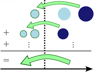
Figure 3. Schematic illustrating the computation of the bubble break-up flux $W_b(D)$ across a particular bubble size $D$ through the appropriate averaging of gaseous mass transfers from individual events as represented by block arrows. Each row corresponds to an individual break-up event. Parent bubbles have a dark fill colour, while child bubbles have a light fill colour. Child bubbles that contribute to $W_b(D)$ are marked with a dark border. For a more comprehensive illustration, refer to figure 11 and the accompanying description in appendix B.

Locality in $W_b$ is quantified using two complementary measures inspired by the concepts of infrared and ultraviolet locality introduced by L'vov & Falkovich (Reference L'vov and Falkovich1992) and Eyink (Reference Eyink2005) for turbulent kinetic energy transfer. First, one is interested in the degree to which incoming contributions to $W_b(D)$ from all parent bubble sizes larger than $D$ arise primarily from sizes only slightly larger than $D$. This metric is termed infrared locality, since infrared radiation has a longer wavelength than visible light. If the rate at which parent bubbles of sizes between $D_p > D$ and $D_p + \mathrm {d} D_p$ transfer mass to bubbles of sizes smaller than $D$ is $I_p(D_p|D) \, \mathrm {d} D_p$, then $W_b(D)$ is the integral of the incoming differential transfer rate $I_p(D_p|D)$ over all parent bubble sizes $D_p > D$. Figure 4(a) illustrates this relation between $I_p$ and $W_b$. With this decomposition of $W_b$, infrared locality may then be quantified by considering how quickly the incoming differential transfer rate $I_p(D_p|D)$ from parent bubbles decays with increasing $D_p$

Definition 2.1 (Infrared locality)

If $W_b(D)$ is written as

(2.8)\begin{equation} W_b(D) = \int_D^\infty \mathrm{d} D_p\, I_p(D_p|D), \end{equation}

then infrared locality describes the rate at which $I_p$ decays from $D_p \gtrsim D$ to $D_p \rightarrow \infty$.

Figure 4. Schematics illustrating infrared locality in the break-up flux $W_b$. $W_b(D)$ may be computed by integrating the incoming differential contributions $I_p(D_p|D)$ from each parent bubble size $D_p > D$. (a) Illustration of this decomposition of $W_b$. In particular, it depicts a system where the incoming differential transfer rate $I_p(D_p|D)$ from parent bubbles varies as $I_p(D_{p1}|D) > I_p(D_{p2}|D) > I_p(D_{p3}|D)$ for $D_{p1} < D_{p2} < D_{p3}$. This variation of $I_p(D_p|D)$ with $D_p$ is graphically depicted in (b). The limiting power-law exponent $\gamma _p$ in (b) describes the behaviour $I_p(D_p\rightarrow \infty |D)$. This exponent is revisited in the relations (4.7) and (4.15).

The variation of $I_p(D_p|D)$ with $D_p$ for an infrared local system is schematically illustrated in figure 4(b).

Second, one is interested in the degree to which outgoing contributions to $W_b(D)$ due to all child bubble sizes smaller than $D$ are due primarily to sizes only slightly smaller than $D$. This metric is correspondingly termed ultraviolet locality. If the rate at which child bubbles of sizes between $D_c$ and $D_c + \mathrm {d} D_c < D$ receive mass from bubbles of sizes larger than $D$ is $I_c(D_c|D) \: \mathrm {d} D_c$, then $W_b(D)$ is the integral of the outgoing differential transfer rate $I_c(D_c|D)$ over all child bubble sizes $D_c < D$. Figure 5(a) illustrates this relation between $I_c$ and $W_b$. With this decomposition of $W_b$, ultraviolet locality may then be quantified by determining how quickly the outgoing differential transfer rate $I_c(D_c|D)$ to child bubbles decays with decreasing $D_c$

Definition 2.2 (Ultraviolet locality)

If $W_b(D)$ is written as

(2.9)\begin{equation} W_b(D) = \int_0^D \mathrm{d} D_c\, I_c(D_c|D), \end{equation}

then ultraviolet locality describes the rate at which $I_c$ decays from $D_c \lesssim D$ to $D_c \rightarrow 0$.

Figure 5. Schematics illustrating ultraviolet locality in the break-up flux $W_b$. $W_b(D)$ may be computed by integrating the outgoing differential contributions $I_c(D_c|D)$ due to each child bubble size $D_c < D$. (a) Illustration of this decomposition of $W_b$. In particular, it depicts a system where the outgoing differential transfer rate $I_c(D_c|D)$ to child bubbles varies as $I_c(D_{c1}|D) > I_c(D_{c2}|D) > I_c(D_{c3}|D)$ for $D_{c1} > D_{c2} > D_{c3}$. This variation of $I_c(D_c|D)$ with $D_c$ is graphically depicted in (b). The limiting power-law exponent $\gamma _c$ in (b) describes the behaviour $I_c(D_c\rightarrow 0|D)$. This exponent is revisited in the relations (4.8) and (4.16).

The variation of $I_c(D_c|D)$ with $D_c$ for an ultraviolet local system is schematically illustrated in figure 5(b). To reiterate, these decompositions of $W_b$ into $I_p$ and $I_c$ are two distinct but complementary ways of analysing the contributions to $W_b$ from different bubble sizes. The sum of all $I_p$ values over all eligible parent bubbles $(D_p>D)$ yields $W_b(D)$, as does the sum of all $I_c$ values over all eligible child bubbles $(D_c < D)$.

3.1. The bubble-size distribution

At every location $\boldsymbol {x}$, for every bubble size $D$, and at some time $t$, the number density function $\mathring {f}$ for a bubble population may be constructed by adding a contribution from each bubble $i = 1, \ldots , N_b(t)$ having a centroid location $\boldsymbol {x}_i$ and an equivalent size $D_i$

(3.1)\begin{equation} \mathring{f}\left(\boldsymbol{x},D;t\right) = \sum_{i=1}^{N_b\left(t\right)} \delta\left(\boldsymbol{x}-\boldsymbol{x}_i(t)\right) \delta\left(D-D_i\left(t\right)\right), \end{equation}

where $\delta$ is the Dirac delta function. Note that $\mathring {f}$ is not a probability density function since it is constructed through the accounting of bubbles in a single system snapshot. The probability distribution of bubble sizes $f$ may be obtained by ensemble averaging over statistically independent but similar realizations

(3.2)\begin{equation} f\left(\boldsymbol{x},D;t\right) = \langle\, \mathring{f}\left(\boldsymbol{x},D;t\right)\rangle. \end{equation}

The probabilistic nature of this size distribution results in a break-up flux in § 3.3 that is compatible with a statistical interpretation of the break-up dynamics. Note that the dimensions of $\mathring {f}$ and $f$ are $(\text {length})^{-4}$ since the following constraints are satisfied over some sampling volume $\int _\varOmega \mathrm{d}\kern0.06em\boldsymbol {x} = \mathcal {V}$ that always contains all $N_b(t)$ bubbles

(3.3a,b)\begin{equation} N_b\left(t\right) = \int_\varOmega \mathrm{d}\kern0.06em\boldsymbol{x} \int_0^\infty \mathrm{d} D\, \mathring{f}\left(\boldsymbol{x},D;t\right),\quad \left\langle N_b\left(t\right) \right\rangle = \int_\varOmega \mathrm{d}\kern0.06em\boldsymbol{x} \int_0^\infty \mathrm{d} D\, f\left(\boldsymbol{x},D;t\right). \end{equation}

Here, the volume-integration $(\int _\varOmega \mathrm {d}\kern0.06em\boldsymbol {x} \, \cdot )$ and ensemble-averaging $(\langle \cdot \rangle )$ operations commute only if $\varOmega$ and $\mathcal {V}$ are identical over all the ensemble realizations.

While many flows, such as breaking waves, are intrinsically statistically unsteady and inhomogeneous, smaller-scale dynamics with faster time scales relative to larger-scale developments may evolve very similarly to statistically stationary and homogeneous flows, as suggested in hypothesis A.1 in appendix A.1. This smaller-scale dynamics occurs in small, localized regions of turbulent flows with sufficient scale separation. This approximation of quasi-stationarity and quasi-homogeneity implies

(3.4)\begin{equation} f\left(\boldsymbol{x},D;t\right) \approx f(D). \end{equation}

In other words, the bubble-size distribution of a statistically stationary and homogeneous turbulent bubbly flow at small and intermediate bubble sizes may shed light on what might be the universal characteristics of a bubble population at small and intermediate bubble sizes in small, localized regions of turbulent bubbly flows with sufficient scale separation, and vice versa.

3.2. The population balance equation

The population balance equation was introduced by Smoluchowski (Reference Smoluchowski1916, Reference Smoluchowski1918), Landau & Rumer (Reference Landau and Rumer1938), Melzak (Reference Melzak1953), Williams (Reference Williams1958), Friedlander (Reference Friedlander1960a,Reference Friedlanderb), Filippov (Reference Filippov1961), Randolph & Larson (Reference Randolph and Larson1962), Fredrickson & Tsuchiya (Reference Fredrickson and Tsuchiya1963) and Behnken, Horowitz & Katz (Reference Behnken, Horowitz and Katz1963) in their respective fields. It is used here to describe the evolution of the bubble-size distribution $f(\boldsymbol {x},D;t)$ in the four-dimensional phase space comprising the three spatial dimensions $\boldsymbol {x}=(x_1,x_2,x_3)$ and the bubble-size dimension $D$ as follows (Hulburt & Katz Reference Hulburt and Katz1964; Randolph Reference Randolph1964)

(3.5)\begin{align} &\frac{\partial \left[f\left(\boldsymbol{x},D;t\right) D^3 \right]}{\partial t} + \frac{\partial \left[v_i\left(\boldsymbol{x},D;t\right) f\left(\boldsymbol{x},D;t\right) D^3 \right]}{\partial x_i} + \frac{\partial \left[v_D\left(\boldsymbol{x},D;t\right) f\left(\boldsymbol{x},D;t\right) D^3 \right]}{\partial D} \nonumber\\ &\quad = H(\boldsymbol{x},D;t), \end{align}

for some model term $H$ that includes the effects of break-up, coalescence, entrainment and other effects. Here, $v_i$ and $v_D$ represent the velocities of the bubble-volume-weighted probability density function, $f\kern0.02em D^3$, in phase space along the spatial and bubble-size dimensions, respectively. The $D^3$-weighting enables the equation to be written in conservative form (Martínez-Bazán et al. Reference Martínez-Bazán, Rodríguez-Rodríguez, Deane, Montañes and Lasheras2010; Saveliev & Gorokhovski Reference Saveliev and Gorokhovski2012) in the incompressible limit where mass and volume are equivalent, since bubble mass is conserved by break-up and coalescence events. Following the arguments of quasi-stationarity and quasi-homogeneity leading to (3.4), one may simplify (3.5) to

(3.6)\begin{equation} \underbrace{\frac{\mathrm{d} \left[v_D(D) f(D) D^3 \right]}{\mathrm{d} D}}_{\text{local transport}} = \underbrace{H(D)}_{\substack{\text{source and sink terms,}\\\text{and non-local transport}}}. \end{equation}

These mechanisms are schematically illustrated in figure 6, which depicts the movement of $f\kern0.02em D^3$ in $D$-space, and are further discussed in appendix C.1. In summary, the phase-space-based form of the population balance equation, (3.6), distinguishes the contributions of local and non-local bubble-mass transport. As explained in appendix B, individual break-up (and coalescence) events are non-local in size space. However, the ensemble-averaged dynamics may be approximated as size local if it satisfies infrared and ultraviolet locality, as discussed in § 2.3. These concepts are appropriate particularly in the limit where the subspace of initial conditions for a bubbly system corresponding to an initial collection of large bubbles is sufficiently sampled. If a quasi-stationary limit exists for the system, then subsequent bubble break-up would lead to a continuous distribution for $f(D)$ after the transient dynamics has passed, as opposed to a discrete distribution comprising a finite number of Dirac delta functions in bubble-size space. Then, if the source and sink mechanisms are neglected, one may re-interpret the terms in (3.6) as

(3.7)\begin{equation} \underbrace{\frac{\mathrm{d} \left[v_D(D) f(D) D^3 \right]}{\mathrm{d} D}}_{\substack{\text{local transport approximation for}\\\text{break-up and/or coalescence}}} = \underbrace{H(D)}_{\substack{\text{error of local}\\\text{transport approximation}}}. \end{equation}

Figure 6. Schematic illustrating the physical significance of the terms in (3.6). Local transport denoted by the lightly shaded block arrows corresponds to the left-hand side term, while the remaining mechanisms denoted by the dark block arrows correspond to the right-hand side term.

The population balance equation (3.5) is often alternatively written, in the limit where mass-transfer processes such as dissolution that would cause individual bubble sizes to continuously increase or decrease with time may be neglected, as

(3.8)\begin{align} &\frac{\partial \left[f\left(\boldsymbol{x},D;t\right) D^3 \right]}{\partial t} + \frac{\partial \left[v_i\left(\boldsymbol{x},D;t\right) f\left(\boldsymbol{x},D;t\right) D^3 \right]}{\partial x_i} \nonumber\\ &\quad = T_b\left(\boldsymbol{x},D;t\right) + T_c\left(\boldsymbol{x},D;t\right) + T_s\left(\boldsymbol{x},D;t\right) \end{align}

for some model terms $T_b$, $T_c$ and $T_s$ corresponding to break-up, coalescence and other sources and sinks, respectively. Once again, (3.8) may be simplified to

(3.9)\begin{equation} 0 = \underbrace{T_b(D)}_{\text{break-up}} + \underbrace{T_c(D)}_{\text{coalescence}} + \underbrace{T_s(D)}_{\substack{\text{other sources}\\\text{and sinks}}}. \end{equation}

The kernel-based form of the population balance equation (3.9) isolates the contributions to bubble-mass transport from individual physical processes. Since break-up and coalescence processes do not create or destroy bubble mass, or bubble volume in the incompressible limit, $T_b(D)$ and $T_c(D)$ must individually satisfy the conservation of bubble mass; for example

(3.10)\begin{equation} \int_0^\infty \mathrm{d} D\, T_b(D) = 0.\end{equation}

Recalling the assumptions in § 2.2, $T_c(D)$ is assumed to be negligible, while $T_s(D)$ is assumed to be active only at small $(D < L_{H})$ and large $(D \sim L)$ bubble sizes. Thus, at intermediate bubble sizes, only $T_b(D)$ is in play. The common model kernel for $T_b(D)$ is the subject of the next subsection. At these intermediate sizes, one may compare (3.7) with (3.9) to approximately obtain, in the limit of size-local break-up,

(3.11)\begin{equation} \underbrace{-\frac{\mathrm{d} \left[v_D(D) f(D) D^3 \right]}{\mathrm{d} D}}_{\text{local transport approximation}} = \underbrace{T_b(D)}_{\text{break-up}}. \end{equation}

The bubble break-up process may then be modelled by an appropriate velocity in bubble-size space, $v_D(D)$, as will be further discussed in § 5.1. Quasi-stationarity and quasi-homogeneity also imply that both terms in (3.11) are zero. In other words, the rate of increase of the number of bubbles of size $D$ due to the break-up of larger bubbles is dynamically balanced by the rate of decrease due to break-up into smaller bubbles. It is further shown in § 4 that this corresponds to the self-similarity of $W_b(D)$ in the intermediate bubble-size subrange $L_{H} \ll D \ll L$, which emerges when there is a sufficient separation of scales.

3.3. The model binary break-up kernel and the corresponding break-up flux

Assuming that all break-up events are independent of one another, i.e. that they follow a Markovian (memoryless) stochastic process where each break-up event is independent of all previous events, and that only binary break-up events occur, a model form for the break-up kernel $T_b(D)$ may be constructed as follows (e.g. Filippov Reference Filippov1961; Valentas & Amundson Reference Valentas and Amundson1966; Valentas et al. Reference Valentas, Bilous and Amundson1966; Coulaloglou & Tavlarides Reference Coulaloglou and Tavlarides1977; Ramkrishna Reference Ramkrishna1985; Martínez-Bazán et al. Reference Martínez-Bazán, Montañés and Lasheras1999a; Martínez-Bazán, Montañés & Lasheras Reference Martínez-Bazán, Montañés and Lasheras1999b; Chan et al. Reference Chan, Dodd, Johnson, Urzay and Moin2018a)

(3.12)\begin{equation} T_b(D) = \int_D^\infty \mathrm{d} D_p\, q_b(D|D_p) g_b(D_p) f(D_p) D^3 - g_b(D) f(D) D^3. \end{equation}

The first term on the right-hand side is a source (birth) term due to the break-up of bubbles of sizes larger than $D$, while the second term is a sink (death) term due to the break-up of bubbles of size $D$ into smaller bubbles. The differential break-up rate $g_b (D) f (D)$ is the expected differential rate of break-up events per unit domain volume for bubbles of size $D$, which is modelled as being proportional to the average number of bubbles of size $D$ per unit domain volume and unit size, $f(D)$. Then, $g_b(D)$ is the characteristic break-up frequency of a bubble of size $D$. Also, $q_b(D|D_p)$ is the probability that a bubble of size $D_p$ breaks into a bubble of size $D$ and another bubble of complementary volume such that the total gaseous volume remains constant through the break-up event. Several properties of $q_b(D_c|D_p)$ that will facilitate subsequent derivations are introduced in appendix C.2. Non-binary break-up events are addressed in appendix D.1.

The corresponding break-up flux $W_b(D)$ may be interpreted in two complementary ways, recalling the concepts introduced at the end of § 2.3. First, it describes the net loss of mass from bubbles of sizes larger than $D$ due to the break-up process modelled by $T_b(D)$, if one decomposes $W_b$ into its incoming contributions from various parent bubbles. Second, it describes the net gain in mass in bubbles of sizes smaller than $D$, if one decomposes $W_b$ into its outgoing contributions to various child bubbles. From (3.10), it is evident that these two quantities are equal in magnitude, leading to the following equivalent definitions for the break-up flux

(3.13)\begin{equation} W_b(D) = \int_0^D \mathrm{d} D_c\, T_b(D_c) = -\int_D^\infty \mathrm{d} D_p\, T_b(D_p). \end{equation}

Note that this implies in turn that

(3.14)\begin{equation} \frac{\mathrm{d} W_b(D)}{\mathrm{d} D} = T_b(D). \end{equation}

Observe the parallels between (3.11) and (3.14), which will be addressed in § 5.1.

One may show that $W_b$ satisfies

(3.15)\begin{equation} W_b(D) = \int_0^D \mathrm{d} D_c\, D_c^3 \int_D^\infty \mathrm{d} D_p\, q_b \left(D_c|D_p\right) g_b(D_p) f(D_p). \end{equation}

A detailed derivation is provided in appendix C.2. Note that the dimensions of $W_b$ are $(\text {time})^{-1}$. Note, also, that $W_b(D)$ has been expressed in terms of integrals with limits involving $D$, similar to the expressions (2.8) and (2.9). One may then directly infer that

(3.16)\begin{gather} I_p(D_p|D) = \int_0^D \mathrm{d} D_c\, D_c^3 q_b \left(D_c|D_p\right) g_b(D_p) f(D_p), \end{gather}

(3.17)\begin{gather}I_c(D_c|D) = \int_D^\infty \mathrm{d} D_p\, D_c^3 q_b \left(D_c|D_p\right) g_b(D_p) f(D_p). \end{gather}

The analysis of the constituent terms in these quantities is the subject of the next section.

It is emphasized again that the break-up flux $W_b$ averages the transfer of bubble mass over many break-up events through the ensemble-averaging operation discussed in § 3.1. Assuming each event occurs independently, (3.15) may be interpreted as the summation of the bubble-mass (or gaseous volume) transfer $q_b(D_c|D_p) D_c^3$, multiplied by the average differential break-up rate $g_b(D_p)f(D_p)$, over all relevant parent and child bubble sizes. This is reiterated using concrete examples in appendix B.

4.1. Uniform distribution in bubble-volume space

Consider, first, the uniform distribution in bubble-volume space ($D^3$-space)

(4.4)\begin{equation} q_b\left(D_c^3|D_p^3\right) = \begin{cases} \dfrac{2}{D_p^3}, & 0 \leqslant D_c^3 \leqslant D_p^3,\\ 0, & D_p^3 < D_c^3, \end{cases} \end{equation}

where the factor of 2 arises from the assumption of binary break-up. From the properties of $q_b$ discussed in appendix C.2, this is equivalent to the following distribution in bubble-size space ($D$-space)

(4.5)\begin{equation} q_b(D_c|D_p) = \begin{cases} \dfrac{6D_c^2}{D_p^3}, & 0 \leqslant D_c \leqslant D_p,\\ 0, & D_p < D_c, \end{cases} \end{equation}

where the additional factor of 3 arises from the change in variables from $D^3$ to $D$. With the available scalings for $q_b$ and $g_b f$, the relations (3.16) and (3.17) yield

(4.6a,b)\begin{align} I_p(D_p|D) \sim \int_0^D \mathrm{d} D_c\, D_c^5 D_p^{-7} \sim D^6 D_p^{-7}, \quad I_c(D_c|D) \sim \int_D^\infty \mathrm{d} D_p\, D_c^5 D_p^{-7} \sim D_c^5 D^{-6}. \end{align}

Observe that $I_p$ and $I_c$ rapidly decrease as $D_p\rightarrow \infty$ and $D_c\rightarrow 0$, respectively, indicating that $W_b$ may be reasonably approximated as size local. More specifically, the limits

(4.7)\begin{equation} I_p(D_p|D) \sim D_p^{\gamma_p} \sim D_p^{-7}, \end{equation}

(4.8)\begin{equation}I_c(D_c|D) \sim D_c^{\gamma_c} \sim D_c^{5} \end{equation}

hold as $D_p \rightarrow \infty$ and $D_c \rightarrow 0$, respectively. The exponents $\gamma _p$ and $\gamma _c$ were referenced earlier in figures 4(b) and 5(b), respectively. Note that these relations hold even at $D_p \sim D$ and $D_c \sim D$, respectively, because $q_b$ is separable in $D_p$ and $D_c$. Thus, a stronger statement on locality may be made in the case of the uniform distribution; since

(4.9)\begin{equation} W_b(D) \sim \left(\int_0^D \mathrm{d} D_c\, D_c^5 \right) \times \left( \int_D^\infty \mathrm{d} D_p\, D_p^{-7}\right) \end{equation}

may be expressed as the separable product of two integrals, one may further conclude that $W_b(D)$ may be directly approximated by a movement of bubble mass in bubble-size space from some bubble size only slightly larger than $D$ to some bubble size only slightly smaller than $D$. Finally, as a self-consistency check, one may obtain the scaling of $W_b(D)$ with $D$

(4.10)\begin{equation} W_b(D) \sim \int_0^D \mathrm{d} D_c \, D_c^5 D^{-6} \sim \int_D^\infty \mathrm{d} D_p\, D^6 D_p^{-7} \sim D^6 D^{-6} \sim \text{constant}. \end{equation}

If the underlying energy flux in the surrounding turbulence is scale invariant within an inertial subrange, and the break-up probability is chosen to be size invariant in a corresponding intermediate range of bubble sizes, then the resulting bubble break-up flux is size invariant, confirming the presence of an intermediate size subrange where the break-up process is self-similar in nature. Self-similarity is compatible with the assumption of statistical quasi-stationarity and quasi-homogeneity as evidenced by (3.9) and (3.14), assuming only $T_b$ is active on the right-hand side of (3.9) in this intermediate size subrange. The potential non-stationarity of a non-self-similar break-up process is further addressed in appendix D.2.

4.2. Beta distribution in bubble-volume space

Recall from § 3.3 that the break-up probability is symmetric in bubble-volume space. The beta distribution that satisfies this constraint can take only a single shape parameter $\alpha$, and may be expressed in bubble-volume space, or $D^3$-space, as

(4.11)\begin{align} q_b(D_c^3|D_p^3) = \begin{cases} 2D_c^{3(\alpha-1)}\left(D_p^3-D_c^3\right)^{\alpha-1}D_p^{-6(\alpha-1)-3}/B(\alpha,\alpha), & 0 \leqslant D_c^3 \leqslant D_p^3,\\ 0, & D_p^3 < D_c^3, \end{cases} \end{align}

where $B(\alpha ,\alpha )$ is the beta function (Abramowitz & Stegun (Reference Abramowitz and Stegun1964), § 6.2), which is a normalization constant for the beta distribution with shape parameter $\alpha$, and the factor of 2 arises from the assumption of binary break-up. This distribution is plotted in figure 7 for several values of $\alpha$. Note that the uniform distribution is recovered when $\alpha =1$. The beta distribution is defined only for $\alpha > 0$. When $0 < \alpha < 1$, the distribution is U-shaped and goes to infinity at the endpoints of the domain, thus favouring the formation of bubbles of unequal sizes. The formation of these bubbles is permitted in the infinite-Weber-number limit where the Hinze scale is zero, as discussed in the introduction. For practical flows with finite integral-scale Weber numbers, the favourable formation of bubbles of sizes smaller than the Hinze scale may not be as plausible, and a more precise surrogate model for $q_b$ may have to involve a truncated U-shaped beta distribution, or an M-shaped distribution. Nevertheless, the U-shaped beta distribution should remain an adequate surrogate model for parent bubbles of sizes $L_n$ in the intermediate size subrange $L_{H} \ll L_n \ll L$ and sufficiently larger than the Hinze scale. When $\alpha > 1$, the distribution is inverted-$U$-shaped and goes to zero at the endpoints, thus favouring the formation of bubbles of equal sizes. The beta distribution is thus a reasonable surrogate model for most observed and modelled break-up distributions, except for the class of M-shaped distributions. One such distribution was introduced by Wang, Wang & Jin (Reference Wang, Wang and Jin2003); see the reviews cited in the preamble of this section for more examples. The analogue of (4.11) in bubble-size space, or $D$-space, is

(4.12)\begin{equation} q_b(D_c|D_p) = \begin{cases} 6D_c^{3\alpha-1}(D_p^3-D_c^3)^{\alpha-1}D_p^{3-6\alpha}/B(\alpha,\alpha), & 0 \leqslant D_c^3 \leqslant D_p^3,\\ 0, & D_p^3 < D_c^3. \end{cases} \end{equation}

With the available scalings for $q_b$ and $g_b f$, the relations (3.16) and (3.17) yield

(4.13)\begin{gather} I_p(D_p|D) \sim \int_0^D \mathrm{d} D_c\, \frac{D_c^{3\alpha+2}}{(D_p^3-D_c^3)^{1-\alpha}} D_p^{-1-6\alpha} \sim D_p^{-1} \int_0^{D^3/D_p^3} \mathrm{d}\kern0.06em x\, x^\alpha (1-x)^{\alpha-1}, \end{gather}

(4.14)\begin{gather}I_c(D_c|D) \sim \int_D^\infty \mathrm{d} D_p\, \frac{D_p^{-1-6\alpha}}{(D_p^3-D_c^3)^{1-\alpha}} D_c^{3\alpha+2} \sim D_c^{-1} \int_0^{D_c^3/D^3} \mathrm{d}\kern0.06em x\, x^\alpha (1-x)^{\alpha-1}. \end{gather}

The final integrals in (4.13) and (4.14) are the incomplete beta functions $B_{D^3/D_p^3}(\alpha +1,\alpha )$ and $B_{D_c^3/D^3}(\alpha +1,\alpha )$, respectively (Abramowitz & Stegun (Reference Abramowitz and Stegun1964), §§ 6.6.1 and 26.5.3). The results discussed in § 4.1 are exactly recovered when $\alpha =1$. The expressions in (4.13) and (4.14) are plotted in arbitrary units as functions of $D_p/D$ and $D_c/D$, respectively, in figure 8. As $\alpha$ increases, the rates of decay of $I_p$ and $I_c$ as $D_p\rightarrow \infty$ and $D_c\rightarrow 0$, respectively, increase, indicating that as break-up events involving child bubbles of similar sizes are increasingly favoured, the locality of the break-up process correspondingly increases. At small $\alpha$, where the most likely break-up events involve child bubbles of very different sizes, the cascade is diffuse, or leaky, and the bubble break-up flux is less local. Also, for sufficiently large $D_p$ and sufficiently small $D_c$, (4.13) and (4.14) may respectively be approximated as

(4.15)\begin{gather} I_p(D_p|D) \approx \frac{D_p^{-1-6\alpha}}{D_p^{3(1-\alpha)}} \sim D_p^{-4-3\alpha} \sim D_p^{\gamma_p}, \end{gather}

(4.16)\begin{gather}I_c(D_c|D) \approx D_c^{3\alpha+2} \sim D_c^{\gamma_c}. \end{gather}

Recall that the exponents $\gamma _p$ and $\gamma _c$ were referenced earlier in figures 4(b) and 5(b), respectively. Note, also, that in these limits, $I_p$ decays at least as quickly as $D_p^{-4}$, and $I_c$ grows at least as quickly as $D_c^2$, so the break-up flux is always at least quasi-local regardless of $\alpha$, for values of $\alpha$ where the beta distribution is defined. Once again, the results of § 4.1 are recovered – in an exact fashion – for $\alpha =1$. Note, in addition, that a bubble break-up process best described by an M-shaped distribution may be modelled by a superposition of two bubble-mass fluxes due to two $q_b$ values with different $\alpha$ values. Since each bubble-mass flux is always at least quasi-local regardless of $\alpha$, this implies that M-shaped distributions also result in a net quasi-local flux. Finally, one may also examine the dependence of $W_b(D)$ on $D$ as a self-consistency check

(4.17)\begin{align} W_b(D) &\sim \int_0^D \mathrm{d} D_c\, \left[ D_c^{-1} \int_0^{D_c^3/D^3} \mathrm{d}\kern0.06em x\, x^\alpha (1-x)^{\alpha-1} \right] \nonumber\\ &\sim \int_D^\infty \mathrm{d} D_p\, \left[ D_p^{-1} \int_0^{D^3/D_p^3} \mathrm{d}\kern0.06em x\, x^\alpha (1-x)^{\alpha-1} \right] \nonumber\\ &\sim \int_0^1 \mathrm{d} y \left[ y^{-1} \int_0^{y^3} \mathrm{d}\kern0.06em x\, x^\alpha (1-x)^{\alpha-1} \right] \nonumber\\ &\sim \text{constant}, \end{align}

which reveals, as expected, an intermediate bubble-size subrange for the bubble break-up flux where the break-up process is self-similar in nature, if $\alpha$ is constant over the size subrange. Once again, self-similar behaviour of $W_b$ is compatible with the statistical quasi-stationarity and quasi-homogeneity of the system $(T_b = 0)$. The potential non-stationarity of a non-self-similar break-up process is further addressed in appendix D.2.

Figure 7. The symmetric beta distribution in $D^3$-space (4.11) for various shape parameters $\alpha$.

Figure 8. Integrands of $W_b$ demonstrating the extent of (a) infrared locality using (4.13) and (b) ultraviolet locality using (4.14) after substituting the symmetric beta distribution with various shape parameters $\alpha$ for the probability distribution of child bubble volumes $q_b$, as well as scalings for the differential bubble break-up rate $g_b f$ corresponding to a turbulent break-up mechanism. Since the proportionality constants are dropped in (4.13) and (4.14), the integrands here are plotted in arbitrary units, with the values at $D_p = D$ (for (a)) and $D_c = D$ (for (b)) fixed at unity. The power-law fits at large $D_p/D$ and small $D_c/D$ correspond to the scaling limits in (4.15) and (4.16) for $\alpha =1/5$ and $\alpha =5$.

4.3. Revisiting some of the assumptions in the bubble break-up formalism

Note that the findings of this work assume that all break-up events are binary in nature. The binary break-up assumption precludes the formation of satellite bubbles, which might be assumed to decrease the locality of the resulting bubble-mass transfer and also disrupt self-similarity. It turns out, however, that locality and self-similarity remain plausible in such a scenario. Non-binary break-up events are addressed in appendix D.1. As mentioned earlier, appendix D.2 discusses non-self-similar break-up mechanisms, which may be relevant in systems without sufficient scale separation. It turns out that locality remains relatively robust even in the absence of self-similarity.

The extent of locality in the break-up flux $W_b(D)$, in particular the respective scalings of $I_p(D_p|D)$ and $I_c(D_c|D)$ with $D_p$ and $D_c$, will be examined in Part 2 via a direct evaluation of the flux from all relevant break-up events in a breaking-wave simulation.

5.1. Relations between bubble-mass and spectral energy flux models

The break-up flux $W_b(D) = \int _0^D \mathrm {d} D_c\, T_b(D_c)$ describes the average movement of bubble mass ${\sim }f(D)D^3$ in bubble-size space ($D$-space) as governed by the population balance equation given in (3.6) and (3.9), where the rate of change of $f(D)D^3$ due to break-up is $T_b(D)$, recalling from the introduction that mass and volume are assumed to be equivalent in the incompressible limit. This is analogous to how the transfer flux $W(k) = \int _0^k \mathrm {d} k'\, T(k')$ describes the movement of turbulent kinetic energy $E(k)$ in wavenumber space ($k$-space) based on the spectral turbulent kinetic energy equation (Batchelor Reference Batchelor1953)

(5.1)\begin{equation} \frac{\partial E(k,t)}{\partial t} = T(k,t) - 2\nu_l k^2 E(k,t), \end{equation}

where the rate of change of $E(k)$ due to interscale transfer is $T(k)$, and the time dependence drops off in the quasi-stationary limit. In particular, the double-integral form of the break-up flux (3.15) is reminiscent of the spectral energy transfer model of Heisenberg (Reference Heisenberg1948a,Reference Heisenbergb), where $W(k)$ is modelled as a separable product of integrals

(5.2)\begin{equation} W(k) \sim \left( \int_0^k \mathrm{d} k' E(k') {k'}^2 \right) \times \left( \int_k^\infty \mathrm{d} k'' \sqrt{\frac{E(k'')}{{k''}^3}} \right). \end{equation}

By substituting the inertial subrange scaling $E(k) \sim k^{-5/3}$ into (5.2), one obtains ${k'}^{-5/3} {k'}^2 \sim {k'}^{1/3}$ and $\sqrt {{k''}^{-5/3}{k''}^{-3}} \sim {k''}^{-7/3}$ for the scalings of the two integrands, suggesting some degree of infrared and ultraviolet locality, respectively. Remarkably, it turns out that these model limits agree with the scalings obtained in the analyses by Eyink (Reference Eyink2005), Eyink & Aluie (Reference Eyink and Aluie2009) and Aluie & Eyink (Reference Aluie and Eyink2009) for the turbulent energy cascade for a monofractal velocity field, as well as an earlier analysis by Kraichnan (Reference Kraichnan1971) based on closure approximations that also introduces a measure of locality and earlier investigations by Zhou (Reference Zhou1993a,Reference Zhoub) based on numerical simulations. Note that these rates of decay are slower than those obtained in §§ 4.1 and 4.2 for the bubble-mass flux integrands, suggesting that the turbulent bubble-mass cascade may be more strongly local than the turbulent energy cascade. One may further evaluate these integrals

(5.3)\begin{equation} W(k) \sim \int_0^k \mathrm{d} k' k'^{1/3} \int_k^\infty \mathrm{d} k'' {k''}^{-7/3} \sim k^{4/3}k^{-4/3} \sim \text{constant}, \end{equation}

in order to see that $W(k)$ has no dependence on $k$, as one would expect for a self-similar energy transfer process. Note that this self-similarity, in turn, implies that the underlying system dynamics is statistically steady or quasi-stationary, since $T(k)$ must then be negligible in the range of scales of interest. An analogous observation was made in the case of the bubble break-up flux in §§ 4.1 and 4.2.

If the true $W(k)$ is quasi-local in $k$-space, then it may be well approximated by a wavenumber-local expression. This brings to mind the quasi-local models of Kovasznay (Reference Kovasznay1948) and Pao (Reference Pao1965, Reference Pao1968). Kovasznay (Reference Kovasznay1948) argued that if $W(k)$ is dependent only on $E(k)$ and $k$, then the only dimensionally consistent expression is

(5.4)\begin{equation} W(k) \sim \left[E(k)\right]^{3/2} k^{5/2}. \end{equation}

Subsequently, Pao (Reference Pao1965, Reference Pao1968) allowed $W(k)$ to depend on $\varepsilon$ as well. If it is further assumed that $W(k)$ is linear in $E(k)$, then it follows from dimensional arguments that

(5.5)\begin{equation} W(k) \sim \varepsilon^{1/3} k^{5/3} E(k). \end{equation}

In a similar fashion, $W_b(D)$ may be justifiably modelled by an expression local in $D$-space if there is sufficient quasi-locality in the break-up flux. From a comparison of (3.11) and (3.14), it is clear that the local transport term in the phase-space-based population balance equation provides an appropriate model form for a local $W_b$. Then, one desires an appropriate model for the velocity of $f(D)D^3$ in bubble-size space, $v_D(D)$, such that

(5.6)\begin{equation} W_b(D) \sim v_D(D) f(D) D^3. \end{equation}

If there exists an intermediate bubble-size subrange where $W_b(D)$ is independent of $D$, and $f(D) \sim D^{-10/3}$, then an appropriate model for $v_D(D)$ should satisfy

(5.7)\begin{equation} v_D(D) \sim D^{1/3}. \end{equation}

Note that this is similar to the scaling for the turbulent velocity fluctuations with eddy size $u_D(D) \sim D^{1/3}$. The scaling for $v_D$ was previously postulated by Garrett et al. (Reference Garrett, Li and Farmer2000) on the dimensional grounds that $v_D \sim u_D$, but one should be cognizant of the difference between bubble-size space and eddy-size space. In addition, the term $\partial (v_D f\kern0.02em D^3)/\partial D$ in the original supporting reference (Garrettson Reference Garrettson1973) was used to model a dissolution process, meaning that the model form referenced by Garrett et al. (Reference Garrett, Li and Farmer2000) is applicable only to the change in bubble mass in individual events. Here, the model form for size-local bubble-mass transport is not applicable to individual events, as will be clarified by the discussion in appendix B. The locality of the corresponding bubble-mass flux must necessarily be interpreted in an averaged sense, as all turbulent cascades should be. In turn, the model velocity $v_D$ strictly describes the averaged break-up dynamics in small, localized regions of turbulent bubbly flows with sufficient scale separation.

To close this discussion, recall the scaling for the break-up frequency $g_b(D) \sim D^{-2/3}$, which may be interpreted as the inverse of the characteristic break-up time of bubbles of size $D$. If one assumes that the flux $W_b(D)$ is effectively described by a size-space velocity $v_D(D)$ such that a characteristic size interval $D$ is travelled in this characteristic time, then one may write $v_D(D) \sim g_b(D)D$, and thus $W_b(D) \sim g_b(D)f(D)D^4$. The scaling $g_b(D) f(D) \sim D^{-4}$ is thus seen to follow directly from the assumption of a quasi-local and self-similar bubble break-up flux. The scaling of Garrett et al. (Reference Garrett, Li and Farmer2000) for $f \sim Q \varepsilon ^{-1/3} D^{-10/3}$, obtained via dimensional analysis in an intermediate bubble-size subrange using a steady large-scale entrainment rate $Q$, is also a direct consequence of quasi-locality and self-similarity in the bubble-mass flux, with the additional consideration that $Q \sim W_b$. This exhibits a clear parallel to the turbulent energy cascade, where it is also typically assumed that the energy production and cascade rates are of the same order of magnitude. Some of these ideas are summarized in the schematic on bubble-mass transport in figure 9. Further remarks on $Q$ are provided in appendix E.

Figure 9. Schematic of local transport of bubble mass ${\sim } f\kern0.02em D^3$ in $D$-space. The large-scale entrainment rate $Q$ is directly related to the bubble-mass flux $W_b \sim v_D\, f\kern0.06em D^3 \sim g_b \,f\kern0.02em D^4$.

Figure 10. Schematic illustrating subgrid-scale modelling in turbulent bubbly flows.

5.2. Implications for subgrid-scale modelling

Aside from providing a theoretical basis for the scalings for $f$ and $v_D$ proposed by Garrett et al. (Reference Garrett, Li and Farmer2000) through connections to the characteristic break-up frequency $g_b$ (Kolmogorov Reference Kolmogorov1949; Hinze Reference Hinze1955; Martínez-Bazán et al. Reference Martínez-Bazán, Montañés and Lasheras1999a), this work has also posited that the bubble break-up cascade provides a universal description of the bubble break-up dynamics at small and intermediate bubble sizes in small, localized regions of turbulent bubbly flows with sufficient scale separation. For example, the break-up flux in these small, localized regions should be constant in an intermediate subrange of bubble sizes $L_{H} \ll L_n \ll L$, provided the surrounding turbulence is sufficiently energetic. Universality simplifies the task of subgrid-scale modelling in turbulent two-phase flows with a large separation of scales, and lends legitimacy to a universal subgrid-scale model in the spirit of LES of turbulent single-phase flows. In traditional LES, large-scale turbulent motions and flow structures are resolved, while small-scale motions and structures are modelled. The rationale for this approach is twofold, as discussed succinctly by Rogallo & Moin (Reference Rogallo and Moin1984). Large-scale motions are influenced by the flow geometry and cannot be assumed to have a universal character. They are thus explicitly resolved, along with the bulk of the energy in the flow. Small-scale motions may be assumed to have a universal character and are instead represented by models that dissipate energy in a universal fashion. A similar idea may be applied to turbulent two-phase flows where a separation of scales enables a universal description of the small scales. Large structures of the dispersed phase are explicitly resolved via an interface-tracking or interface-capturing method, while small structures of the dispersed phase are treated as subgrid entities using a Lagrangian point-particle description. If the formation and dynamics of these subgrid bubbles occur in a universal fashion, then simplified models may be used to generate these bubbles through the modelled break-up of larger bubbles. For example, the results of this work suggest that in simulations where the mesh resolution is larger than the expected $L_{H}$, the generation of super-Hinze-scale subgrid bubbles may be modelled via a bubble break-up cascade, as illustrated in figure 10. As noted in the introduction, most sub-Hinze-scale bubbles are expected to be formed by distinct fragmentation mechanisms, such as Mesler entrainment, as well as regular and irregular drop entrainment (Deane & Stokes Reference Deane and Stokes2002; Kiger & Duncan Reference Kiger and Duncan2012; Chan et al. Reference Chan, Urzay and Moin2018b, Reference Chan, Mirjalili, Jain, Urzay, Mani and Moin2019). As such, the generation of sub-Hinze-scale subgrid bubbles will have to be addressed separately in a manner that bypasses the cascade considered in this work (see e.g. Chan et al. Reference Chan, Dodd, Johnson, Urzay and Moin2018a,Reference Chan, Urzay and Moinb, Reference Chan, Mirjalili, Jain, Urzay, Mani and Moin2019; Mirjalili et al. Reference Mirjalili, Chan and Mani2018; Mirjalili & Mani Reference Mirjalili and Mani2020). It is envisioned that distinct subgrid-scale models for sub-Hinze-scale and super-Hinze-scale subgrid bubbles be combined in an additive fashion in order to account for this myriad of fragmentation mechanisms and cover more bases for modelling the formation and dynamics of subgrid bubbles. A detailed formulation of a suitable subgrid-scale model in the context of super-Hinze-scale subgrid bubbles is under development. This model would use both the kernel-based break-up model form (3.15), as well as the phase-space-based break-up model form (5.6).