


1 Introduction
Magnetohydrodynamic (MHD) flows in rectangular ducts, amongst many other geometries, have received significant attention in the past due to their wide application (Shercliff Reference Shercliff1953; Hunt Reference Hunt1965), especially in the cooling system of poloidal self-cooled blankets (Molokov Reference Molokov1994). It is known that magnetohydrodynamic effects serve to reduce the thermal hydraulic performance of these duct flows by greatly increasing the pressure drop and reducing the heat transfer coefficient through laminarisation of the flow (Hartmann & Lazarus Reference Hartmann and Lazarus1937). An experimental investigation revealed that the transition to a laminar state occurs at
 $Re/Ha\approx 225$
(Brouillette & Lykoudis Reference Brouillette and Lykoudis1967), where
$Re/Ha\approx 225$
(Brouillette & Lykoudis Reference Brouillette and Lykoudis1967), where
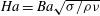 $Ha=Ba\sqrt{{\it\sigma}/{\it\rho}{\it\nu}}$
is the Hartmann number and
$Ha=Ba\sqrt{{\it\sigma}/{\it\rho}{\it\nu}}$
is the Hartmann number and
 $Re$
is the typical hydrodynamic Reynolds number. Here,
$Re$
is the typical hydrodynamic Reynolds number. Here,
 $B$
is the imposed magnetic field,
$B$
is the imposed magnetic field,
 $a$
is the out-of-plane duct depth (in the magnetic field direction), while
$a$
is the out-of-plane duct depth (in the magnetic field direction), while
 ${\it\sigma}$
,
${\it\sigma}$
,
 ${\it\rho}$
and
${\it\rho}$
and
 ${\it\nu}$
are the electrical conductivity, density and kinematic viscosity of the liquid metal, respectively. The stabilizing effect derives from the additional damping in the form of Hartmann braking. In the limit of high magnetic field strength, a very thin boundary layer on the wall perpendicular to the magnetic field direction (known as the Hartmann layer) dominates the friction in an MHD duct flow (Krasnov, Zikanov & Boeck Reference Krasnov, Zikanov and Boeck2012) and the flow becomes quasi-two-dimensional (with 2-D core flow and 3-D flow confined in the boundary layers). In this regime, the induced currents predominantly reside in the Hartmann layer, and hence Joule dissipation is only important in this layer (Pothérat, Sommeria & Moreau Reference Pothérat, Sommeria and Moreau2000). Furthermore, in the context of fusion applications, liquid metals have a very high electrical conductivity (
${\it\nu}$
are the electrical conductivity, density and kinematic viscosity of the liquid metal, respectively. The stabilizing effect derives from the additional damping in the form of Hartmann braking. In the limit of high magnetic field strength, a very thin boundary layer on the wall perpendicular to the magnetic field direction (known as the Hartmann layer) dominates the friction in an MHD duct flow (Krasnov, Zikanov & Boeck Reference Krasnov, Zikanov and Boeck2012) and the flow becomes quasi-two-dimensional (with 2-D core flow and 3-D flow confined in the boundary layers). In this regime, the induced currents predominantly reside in the Hartmann layer, and hence Joule dissipation is only important in this layer (Pothérat, Sommeria & Moreau Reference Pothérat, Sommeria and Moreau2000). Furthermore, in the context of fusion applications, liquid metals have a very high electrical conductivity (
 ${\it\sigma}=O(10^{6})~{\rm\Omega}^{-1}~\text{m}^{-1}$
; Lyon Reference Lyon1952), thus Joule dissipation becomes insignificant when compared to the high heat flux at the plasma-facing wall (Burr et al.
Reference Burr, Barleon, Müller and Tsinober2000). In this case, Hartmann damping plays a greater role in the damping of the 2-D vortices (Mück et al.
Reference Mück, Günther, Müller and Bühler2000). Substantial progress has been made using both experiments and modelling to understand these physical phenomena in various geometries relevant to the cooling ducts of liquid metal fusion blanket. Analytic solutions have been obtained in a number of simple geometries for both conducting and insulating ducts (Müller & Bühler Reference Müller and Bühler2001).
${\it\sigma}=O(10^{6})~{\rm\Omega}^{-1}~\text{m}^{-1}$
; Lyon Reference Lyon1952), thus Joule dissipation becomes insignificant when compared to the high heat flux at the plasma-facing wall (Burr et al.
Reference Burr, Barleon, Müller and Tsinober2000). In this case, Hartmann damping plays a greater role in the damping of the 2-D vortices (Mück et al.
Reference Mück, Günther, Müller and Bühler2000). Substantial progress has been made using both experiments and modelling to understand these physical phenomena in various geometries relevant to the cooling ducts of liquid metal fusion blanket. Analytic solutions have been obtained in a number of simple geometries for both conducting and insulating ducts (Müller & Bühler Reference Müller and Bühler2001).
The cooling process can be assisted either by mixing of the flow via turbulence or vortical structures, or by the acceleration of a near-wall flow. The latter is encountered in MHD duct flows where the Hartmann walls are perfectly electrically conducting and the Shercliff walls are electrically insulating (known as Hunt’s flow; Hunt Reference Hunt1965). In this configuration, high velocity jet flows near the sidewalls give rise to an M-shaped profile. It has been shown previously that an increase in magnetic field intensity generally leads to an improved heat transfer near the walls (Miyazaki et al. Reference Miyazaki, Inoue, Kimoto, Yamashita, Inoue and Yamaoka1986; Cuevas et al. Reference Cuevas, Picologlou, Walker, Talmage and Hua1997; Takahashi et al. Reference Takahashi, Aritomi, Inoue and Matsuzaki1998).
In contrast, when all walls are insulating, the flow presents a flat velocity profile in the core region, monotonically decreasing to zero through the side layers. The flow in this configuration generally features a lower heat transfer from the heated sidewall as compared to the conducting Hartmann wall counterpart (Cuevas et al. Reference Cuevas, Picologlou, Walker, Talmage and Hua1997). It has been reported that the transverse magnetic field tends to inhibit the convective mechanism of heat transfer in an insulated duct flow by as much as 70 % (Gardner & Lykoudis Reference Gardner and Lykoudis1971). Despite the low heat transfer characteristic, insulated ducts offer promising application to fusion blankets due to their low pressure drop (Cuevas et al. Reference Cuevas, Picologlou, Walker, Talmage and Hua1997). Hence it has become a particular interest of researchers to enhance the heat transfer in this flow configuration. Several methods have been proposed to improve the convective heat transfer, but generally the mechanism is the same: either by promoting turbulence or by generating vortical velocity fields in the flow in order to enhance transverse fluid mixing and to reduce thermal boundary layer thickness (Sukoriansky et al. Reference Sukoriansky, Klaiman, Branover and Greenspan1989). Suggested methods to generate these vortices include placement of an obstacle such as a cylinder in the duct (Malang & Tillack Reference Malang and Tillack1995; Hussam & Sheard Reference Hussam and Sheard2013), grid bars (Sukoriansky et al. Reference Sukoriansky, Klaiman, Branover and Greenspan1989; Branover, Eidelman & Nagorny Reference Branover, Eidelman and Nagorny1995) or a wall protrusion (Kolesnikov & Andreev Reference Kolesnikov and Andreev1997). However, the level of turbulence is dependent on the flow conditions. For example, high magnetic fields result in a low bulk flow velocity upstream of the obstacle, which then leads to a complete suppression of wake shedding downstream of the cylinder (Lahjomri, Capéran & Alemany Reference Lahjomri, Capéran and Alemany1993) or turbulence (Shatrov & Gerbeth Reference Shatrov and Gerbeth2010). In the case of a cylinder obstacle, the kinematics of the wake vortices can be enhanced via an active excitation. Hussam, Thompson & Sheard (Reference Hussam, Thompson and Sheard2012b ) reported that the optimum perturbations leading to Kármán vortex shedding are localized in the near-wake region around the cylinder, which can be excited by a cylinder oscillation. Studies have examined cylinder rotation about its own axis (Beskok et al. Reference Beskok, Raisee, Celik, Yagiz and Cheraghi2012; Hussam, Thompson & Sheard Reference Hussam, Thompson and Sheard2012a ), or oscillated in either a transverse direction (Yang Reference Yang2003; Fu & Tong Reference Fu and Tong2004; Celik, Raisee & Beskok Reference Celik, Raisee and Beskok2010) or in line with the incident flow (Griffin & Ramberg Reference Griffin and Ramberg1976). The resulting vorticity field in all cases are similar, despite the different oscillation mechanisms (Beskok et al. Reference Beskok, Raisee, Celik, Yagiz and Cheraghi2012). It has been found that increasing oscillation amplitude leads to a higher convective heat transfer from a hot wall (Yang Reference Yang2003; Beskok et al. Reference Beskok, Raisee, Celik, Yagiz and Cheraghi2012), though the gains become more modest at larger amplitudes (Hussam et al. Reference Hussam, Thompson and Sheard2012a ). Furthermore, substantial improvement in Nusselt number has been observed when the cylinder oscillates with a frequency within the lock-in regime (Fu & Tong Reference Fu and Tong2004), a region over which the cylinder motion governs the wake shedding frequency. An oscillation frequency beyond this lock-in regime leads to a lower convective heat transport (Yang Reference Yang2003; Celik et al. Reference Celik, Raisee and Beskok2010; Beskok et al. Reference Beskok, Raisee, Celik, Yagiz and Cheraghi2012). It is also found that higher oscillation amplitude leads to a lower optimum oscillation frequency (Hussam et al. Reference Hussam, Thompson and Sheard2012a ) and broader primary lock-in regime (Mahfouz & Badr Reference Mahfouz and Badr2000).
In general, a remarkable heat transfer enhancement associated with active excitation has been reported. However, studies relevant to duct heat transfer enhancement in MHD flows are rather scarce. Furthermore, employing a mechanical actuator for such turbulisers in a duct faces significant technical obstacles to a practical implementation. An alternative vorticity generation mechanism is by the use of inhomogeneous wall conductivity, as has been explored by Bühler (Reference Bühler1996). The smoothly transitioned wall conductance inhomogeneity leads to the formation of a quasi-2-D shear layer in the duct. Above a critical Reynolds number, which depends on Hartmann number, this shear layer is strong enough to trigger Kelvin–Helmoltz instabilities (Smolentsev, Vetcha & Moreau Reference Smolentsev, Vetcha and Moreau2012), which result in the wake resembling that of Kármán vortex street. However, this mechanism acts passively on the flow and lacks a means to control the ensuing vorticity.
Alternatively, one can take advantage of the MHD flow characteristics, i.e. the presence of an imposed magnetic field in an electrically conducting flow, to intensify vortical structures by means of electric current injection from an electrode mounted flush with one of the Hartmann walls. The design and implementation of such a system would avoid the complexity of a mechanically actuated turbulence promoter system. Furthermore, the amount and rate of current injection can be actively controlled based on feedback from the flow conditions. Electrical generation of vortices has already been used to generate vortices parallel to the imposed magnetic field by Sommeria (Reference Sommeria1988), Pothérat, Sommeria & Moreau (Reference Pothérat, Sommeria and Moreau2005), Pothérat & Klein (Reference Pothérat and Klein2014) in the study of decaying vortices, flow stability and MHD turbulence, but not yet in a duct arrangement with sidewall heating.
The aim of the present work is to enhance heat transfer from the heated sidewall of an MHD duct by utilizing a passive cylinder wake mechanism augmented with a current injection forcing. Influences of vortex dynamics on heat transfer, pressure drop and efficiency enhancement are examined over a wide range of current injection amplitudes, frequencies and pulse width, magnetic field strength, cylinder gap ratios and electrode positions. We focus on a flow with Reynolds number
 $200\leqslant Re\leqslant 3000$
and friction parameter
$200\leqslant Re\leqslant 3000$
and friction parameter
 $200\leqslant H=n(L/a)^{2}Ha\leqslant 5000$
in a duct with a blockage ratio
$200\leqslant H=n(L/a)^{2}Ha\leqslant 5000$
in a duct with a blockage ratio
 ${\it\beta}=d/2L=0.2$
, where
${\it\beta}=d/2L=0.2$
, where
 $n$
is the number of Hartmann walls (
$n$
is the number of Hartmann walls (
 $n=1$
in the case with a free surface and
$n=1$
in the case with a free surface and
 $n=2$
for a flow between two Hartmann walls),
$n=2$
for a flow between two Hartmann walls),
 $L$
is half of the duct width and
$L$
is half of the duct width and
 $d$
is cylinder diameter. These parameters are chosen as they produce time periodic flows at each gap ratio, permitting investigation of the interaction between the forcing current injection and the natural vortex shedding behind the cylinder. Owing to the fact that there is a limited number of studies on actively excited cylinder wake vortices in an MHD duct flow in the literature, the present investigation will furnish valuable information for the design of efficient heat transport systems in high magnetic field applications.
$d$
is cylinder diameter. These parameters are chosen as they produce time periodic flows at each gap ratio, permitting investigation of the interaction between the forcing current injection and the natural vortex shedding behind the cylinder. Owing to the fact that there is a limited number of studies on actively excited cylinder wake vortices in an MHD duct flow in the literature, the present investigation will furnish valuable information for the design of efficient heat transport systems in high magnetic field applications.

Figure 1. Schematic diagram of the system under investigation. The cylinder spans the duct, with diameter
 $d$
and axis parallel to
$d$
and axis parallel to
 $z$
-direction, and the small circle indicates a point electrode embedded in one of the Hartmann walls.
$z$
-direction, and the small circle indicates a point electrode embedded in one of the Hartmann walls.
This paper is organized as follows: the problem set-up and relevant equations are presented in § 2.1–2.3. A sensitivity study on numerical parameters concerning the grid independence and domain length are presented in § 2.4. In § 3, the results related to heat transfer enhancement are presented. Section 4 is dedicated to the analysis of pressure loss and overall efficiency of the system, followed by conclusions in § 5.
2 Methodology
2.1 Computational set-up
In this investigation a flow of electrically conducting fluid passing over a circular cylinder in a rectangular duct is considered (as depicted in figure 1). The bottom wall of the duct (grey shaded region in figure 1) is maintained at a constant hot temperature of
 ${\it\theta}_{w}$
, while the top wall and inflow have a constant cold temperature of
${\it\theta}_{w}$
, while the top wall and inflow have a constant cold temperature of
 ${\it\theta}_{0}$
. The cylinder is thermally insulated, while the duct sidewalls and the cylinder are each electrically insulated. On the duct walls and the cylinder surface, a no-slip condition is imposed. A fully developed quasi-2-D MHD duct flow is applied at the duct inlet (Pothérat Reference Pothérat2007), defined by
${\it\theta}_{0}$
. The cylinder is thermally insulated, while the duct sidewalls and the cylinder are each electrically insulated. On the duct walls and the cylinder surface, a no-slip condition is imposed. A fully developed quasi-2-D MHD duct flow is applied at the duct inlet (Pothérat Reference Pothérat2007), defined by
 $$\begin{eqnarray}\displaystyle u(y)=\frac{\text{cosh}\sqrt{H}}{\text{cosh}\sqrt{H}-1}\left(1-\frac{\text{cosh}(\sqrt{H}y)}{\text{cosh}\sqrt{H}}\right), & & \displaystyle\end{eqnarray}$$
while at the outlet, a constant reference pressure is imposed and a zero streamwise gradient of velocity is weakly imposed. The transverse distance between the cylinder and the heated wall is characterised by the gap ratio
 $G/d$
. This study considers gap ratios
$G/d$
. This study considers gap ratios
 $G/d=0.5$
,
$G/d=0.5$
,
 $1$
and
$1$
and
 $2$
, with
$2$
, with
 $G/d=2$
corresponding to the duct centreline. The wake flow is modified by means of current injection through an electrode embedded at various locations in the otherwise electrically insulating out-of-plane duct wall. The ratio of cylinder diameter to the duct width (i.e. blockage ratio,
$G/d=2$
corresponding to the duct centreline. The wake flow is modified by means of current injection through an electrode embedded at various locations in the otherwise electrically insulating out-of-plane duct wall. The ratio of cylinder diameter to the duct width (i.e. blockage ratio,
 ${\it\beta}=d/2L$
) is fixed at 0.2 throughout this study. A uniform magnetic field
${\it\beta}=d/2L$
) is fixed at 0.2 throughout this study. A uniform magnetic field
 $B$
is imposed in the axial direction (
$B$
is imposed in the axial direction (
 $z$
-axis).
$z$
-axis).
In the present context, the magnetic Reynolds number
 $Rm$
is low and hence the Lorentz force is diffusive in nature due to the typical low-velocity liquid metal and relatively small length scale (Davidson Reference Davidson2001). The fluctuating induced magnetic field around the externally applied field is negligible, and therefore, the quasi-static approximation is invoked (Roberts Reference Roberts1967). However, Alfvén waves might be generated when either the Hartmann number is sufficiently high or strong current pulses are injected into the flow. Their propagation along the magnetic field is governed by the Lundquist number
$Rm$
is low and hence the Lorentz force is diffusive in nature due to the typical low-velocity liquid metal and relatively small length scale (Davidson Reference Davidson2001). The fluctuating induced magnetic field around the externally applied field is negligible, and therefore, the quasi-static approximation is invoked (Roberts Reference Roberts1967). However, Alfvén waves might be generated when either the Hartmann number is sufficiently high or strong current pulses are injected into the flow. Their propagation along the magnetic field is governed by the Lundquist number
 $S=Ha\,Pr_{m}^{1/2}$
(Lundquist Reference Lundquist1949), where
$S=Ha\,Pr_{m}^{1/2}$
(Lundquist Reference Lundquist1949), where
 $Pr_{m}$
is the magnetic Prandtl number. For liquid metals, the quasi-static approximation holds when
$Pr_{m}$
is the magnetic Prandtl number. For liquid metals, the quasi-static approximation holds when
 $Ha\leqslant O(10^{3})$
(Pothérat & Kornet Reference Pothérat and Kornet2015). Taking this constraint into consideration, the magnetic field intensity was limited to
$Ha\leqslant O(10^{3})$
(Pothérat & Kornet Reference Pothérat and Kornet2015). Taking this constraint into consideration, the magnetic field intensity was limited to
 $H=5000$
(which corresponds to
$H=5000$
(which corresponds to
 $Ha=10^{4}$
for
$Ha=10^{4}$
for
 $n=2$
and
$n=2$
and
 ${\it\alpha}=1$
). It should be noted that the bulk of the present numerical simulations was based on the flow at
${\it\alpha}=1$
). It should be noted that the bulk of the present numerical simulations was based on the flow at
 $H=500$
. Here,
$H=500$
. Here,
 ${\it\alpha}=a/2L$
is the aspect ratio of the duct. It is therefore anticipated that the Alfvén waves, if present, will produce rather limited effects due to strong dissipation. Moreover, current pulses have been used previously to drive quasi-2-D flows (Sommeria Reference Sommeria1988) and no such effect was reported.
${\it\alpha}=a/2L$
is the aspect ratio of the duct. It is therefore anticipated that the Alfvén waves, if present, will produce rather limited effects due to strong dissipation. Moreover, current pulses have been used previously to drive quasi-2-D flows (Sommeria Reference Sommeria1988) and no such effect was reported.
For large interaction parameter, the flow tends towards two-dimensionality (Sommeria & Moreau Reference Sommeria and Moreau1982). Recent evidence of the quasi-two-dimensionality of MHD flows can be found in Krasnov et al. (Reference Krasnov, Zikanov and Boeck2012), Kanaris, Albets, Grigoriadis & Kassinos (Reference Kanaris, Albets, Grigoriadis and Kassinos2013), Rhoads, Edlund & Ji (Reference Rhoads, Edlund and Ji2014). A typical quasi-two-dimensional velocity profile is shown in figure 1, characterised by a flat profile in the core with velocity
 $U_{0}$
and high gradients in the vicinity of the lateral walls (Pothérat Reference Pothérat2007).
$U_{0}$
and high gradients in the vicinity of the lateral walls (Pothérat Reference Pothérat2007).
2.2 Governing equations
In the present investigation, the flow is described by a theoretical model proposed by Sommeria & Moreau (Reference Sommeria and Moreau1982) based on a quasi-2-D assumption where the flow quantities in the 2-D core flow and in the Hartmann layers are averaged along the magnetic field direction to give a modified two-dimensional Navier–Stokes equation augmented by a linear braking term representing friction in the Hartmann layers. This averaging is possible when the so-called two-dimensionalisation time
 $\hat{{\it\tau}}_{2D}={\it\rho}{\it\lambda}^{2}/{\it\sigma}\hat{B}^{2}$
, where
$\hat{{\it\tau}}_{2D}={\it\rho}{\it\lambda}^{2}/{\it\sigma}\hat{B}^{2}$
, where
 ${\it\lambda}=l_{\Vert }/l_{\bot }$
is the ratio of the scales parallel and perpendicular to the magnetic field, i.e. the time for the Lorenz force to act to diffuse momentum of a fluid structure along magnetic field lines (Sommeria & Moreau Reference Sommeria and Moreau1982), is much shorter than any other time scales so that quasi-two-dimensionality is achieved within the flow. The relevant time scales include the time scales for viscous diffusion in both perpendicular and parallel planes, and the inertia time scale. These conditions are attained when both Hartmann number
${\it\lambda}=l_{\Vert }/l_{\bot }$
is the ratio of the scales parallel and perpendicular to the magnetic field, i.e. the time for the Lorenz force to act to diffuse momentum of a fluid structure along magnetic field lines (Sommeria & Moreau Reference Sommeria and Moreau1982), is much shorter than any other time scales so that quasi-two-dimensionality is achieved within the flow. The relevant time scales include the time scales for viscous diffusion in both perpendicular and parallel planes, and the inertia time scale. These conditions are attained when both Hartmann number
 $Ha\gg 1$
and interaction parameter
$Ha\gg 1$
and interaction parameter
 $N\gg 1$
, in which any velocity variations along the magnetic field direction is suppressed almost instantaneously (Pothérat et al.
Reference Pothérat, Sommeria and Moreau2000), and the Hartmann layer is laminar (Pothérat & Schweitzer Reference Pothérat and Schweitzer2011). Here, the interaction parameter is defined as
$N\gg 1$
, in which any velocity variations along the magnetic field direction is suppressed almost instantaneously (Pothérat et al.
Reference Pothérat, Sommeria and Moreau2000), and the Hartmann layer is laminar (Pothérat & Schweitzer Reference Pothérat and Schweitzer2011). Here, the interaction parameter is defined as
 $N=Ha^{2}/Re_{L}$
.
$N=Ha^{2}/Re_{L}$
.
Hartmann number and Reynolds number were varied with
 $200\leqslant H\leqslant 5000$
and
$200\leqslant H\leqslant 5000$
and
 $1500\leqslant Re\leqslant 3000$
. These parameter ranges correspond to
$1500\leqslant Re\leqslant 3000$
. These parameter ranges correspond to
 $50\lesssim N\lesssim 67\,000$
for
$50\lesssim N\lesssim 67\,000$
for
 $n=2$
and
$n=2$
and
 ${\it\alpha}=1$
, which justifies the employment of the SM82 model. Theoretically, the SM82 model is accurate to order max(
${\it\alpha}=1$
, which justifies the employment of the SM82 model. Theoretically, the SM82 model is accurate to order max(
 $Ha^{-1}$
,
$Ha^{-1}$
,
 $N^{-1}$
) (Pothérat et al.
Reference Pothérat, Sommeria and Moreau2005). In the case of rectangular duct flows, the SM82 model has been verified against three-dimensional analytical solutions, where the local error in the velocity profile in the sidewall boundary layer is less than
$N^{-1}$
) (Pothérat et al.
Reference Pothérat, Sommeria and Moreau2005). In the case of rectangular duct flows, the SM82 model has been verified against three-dimensional analytical solutions, where the local error in the velocity profile in the sidewall boundary layer is less than
 $10\,\%$
(Pothérat et al.
Reference Pothérat, Sommeria and Moreau2000). Furthermore, 3-D simulations of MHD wakes behind a cylinder by Mück et al. (Reference Mück, Günther, Müller and Bühler2000) verified the accuracy of the quasi-2-D model at high
$10\,\%$
(Pothérat et al.
Reference Pothérat, Sommeria and Moreau2000). Furthermore, 3-D simulations of MHD wakes behind a cylinder by Mück et al. (Reference Mück, Günther, Müller and Bühler2000) verified the accuracy of the quasi-2-D model at high
 $N$
and
$N$
and
 $Ha$
. This result is further supported by more recent 3-D simulations by Kanaris et al. (Reference Kanaris, Albets, Grigoriadis and Kassinos2013), where at the highest
$Ha$
. This result is further supported by more recent 3-D simulations by Kanaris et al. (Reference Kanaris, Albets, Grigoriadis and Kassinos2013), where at the highest
 $Ha$
investigated, they found maximum errors of the averaged parameters between the quasi-2-D model and the 3-D DNS of
$Ha$
investigated, they found maximum errors of the averaged parameters between the quasi-2-D model and the 3-D DNS of
 $6\,\%$
and
$6\,\%$
and
 $8\,\%$
for the steady and time-dependent flows, respectively. The model has also been found to predict the rate of decay of cylinder wake vortices very well within the high-
$8\,\%$
for the steady and time-dependent flows, respectively. The model has also been found to predict the rate of decay of cylinder wake vortices very well within the high-
 $N$
regime (Hamid et al.
Reference Hamid, Hussam, Pothérat and Sheard2015). It is also worth mentioning that a quasi-2-D model proposed by Smolentsev & Moreau (Reference Smolentsev and Moreau2007) for MHD turbulence based on SM82 has been found to be in excellent agreement with previous experimental results.
$N$
regime (Hamid et al.
Reference Hamid, Hussam, Pothérat and Sheard2015). It is also worth mentioning that a quasi-2-D model proposed by Smolentsev & Moreau (Reference Smolentsev and Moreau2007) for MHD turbulence based on SM82 has been found to be in excellent agreement with previous experimental results.
Introducing the non-dimensional variables and coordinates which are defined from physical variables as
 $$\begin{eqnarray}\left.\begin{array}{@{}c@{}}\displaystyle p=\frac{1}{{\it\rho}{U_{0}}^{2}}\hat{p},\quad \boldsymbol{x}=\frac{1}{L}\hat{\boldsymbol{x}},\quad {\it\theta}=\frac{\hat{{\it\theta}}-\hat{{\it\theta}}_{0}}{\hat{{\it\theta}}_{w}-\hat{{\it\theta}}_{0}},\\ \displaystyle \boldsymbol{u}=\frac{1}{U_{0}}\hat{\boldsymbol{u}},\quad t=\frac{U_{0}}{L}\hat{t},\end{array}\right\}\end{eqnarray}$$
the non-dimensional MHD equations of continuity, momentum and energy are
 $$\begin{eqnarray}\displaystyle & \displaystyle \boldsymbol{{\rm\nabla}}\boldsymbol{\cdot }\boldsymbol{u}=0, & \displaystyle\end{eqnarray}$$
 $$\begin{eqnarray}\displaystyle & \displaystyle \frac{\partial \boldsymbol{u}}{\partial t}=-(\boldsymbol{u}\boldsymbol{\cdot }\boldsymbol{{\rm\nabla}})\boldsymbol{u}-\boldsymbol{{\rm\nabla}}p+\frac{1}{Re_{L}}{\rm\nabla}^{2}\boldsymbol{u}+\frac{L^{2}}{a^{2}}\frac{Ha}{Re_{L}}(\boldsymbol{u}_{0}-n\boldsymbol{u}), & \displaystyle\end{eqnarray}$$
and
 $$\begin{eqnarray}\displaystyle \frac{\partial {\it\theta}}{\partial t}+(\boldsymbol{u}\boldsymbol{\cdot }\boldsymbol{{\rm\nabla}}){\it\theta}=\frac{1}{Pe}{\rm\nabla}^{2}{\it\theta}, & & \displaystyle\end{eqnarray}$$
respectively, where
 $\boldsymbol{u}$
,
$\boldsymbol{u}$
,
 $p$
,
$p$
,
 ${\it\theta}$
and
${\it\theta}$
and
 $\boldsymbol{u}_{0}$
are the velocity, pressure, temperature and forcing velocity field (which in the context of the present study, is a transverse electric current density imposed at the sidewalls), respectively, projected onto a plane orthogonal to the magnetic field,
$\boldsymbol{u}_{0}$
are the velocity, pressure, temperature and forcing velocity field (which in the context of the present study, is a transverse electric current density imposed at the sidewalls), respectively, projected onto a plane orthogonal to the magnetic field,
 $U_{0}$
is peak inlet velocity and
$U_{0}$
is peak inlet velocity and
 $\boldsymbol{{\rm\nabla}}$
is the gradient operator. The dimensionless parameters Reynolds number
$\boldsymbol{{\rm\nabla}}$
is the gradient operator. The dimensionless parameters Reynolds number
 $Re_{L}$
, Hartmann number
$Re_{L}$
, Hartmann number
 $Ha$
and Peclet number
$Ha$
and Peclet number
 $Pe$
are defined as
$Pe$
are defined as
 $$\begin{eqnarray}\left.\begin{array}{@{}c@{}}\displaystyle Re_{L}=U_{0}L/{\it\nu},\\ \displaystyle Ha=Ba\sqrt{{\it\sigma}/{\it\rho}{\it\nu}},\\ \displaystyle Pe=U_{0}L/{\it\kappa}_{T}=Re_{L}Pr,\end{array}\right\}\end{eqnarray}$$
where
 ${\it\kappa}_{T}$
is the thermal diffusivity of the fluid. Prandtl number
${\it\kappa}_{T}$
is the thermal diffusivity of the fluid. Prandtl number
 $Pr={\it\nu}/{\it\kappa}_{T}$
characterizes the ratio of viscous to thermal diffusion in the fluid and
$Pr={\it\nu}/{\it\kappa}_{T}$
characterizes the ratio of viscous to thermal diffusion in the fluid and
 $Pr=0.022$
is used throughout, representative of the eutectic alloy GaInSn. This liquid metal has been employed widely in MHD laboratory experiments, e.g. Frank, Barleon & Müller (Reference Frank, Barleon and Müller2001), Morley et al. (Reference Morley, Burris, Cadwallader and Nornberg2008), Klein, Pothérat & Alferenok (Reference Klein, Pothérat and Alferenok2009). In this paper, Hartmann number is expressed in term of a friction parameter
$Pr=0.022$
is used throughout, representative of the eutectic alloy GaInSn. This liquid metal has been employed widely in MHD laboratory experiments, e.g. Frank, Barleon & Müller (Reference Frank, Barleon and Müller2001), Morley et al. (Reference Morley, Burris, Cadwallader and Nornberg2008), Klein, Pothérat & Alferenok (Reference Klein, Pothérat and Alferenok2009). In this paper, Hartmann number is expressed in term of a friction parameter
 $H=n(L/a)^{2}Ha$
, following Pothérat (Reference Pothérat2007).
$H=n(L/a)^{2}Ha$
, following Pothérat (Reference Pothérat2007).
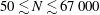
The electric current is injected in alternating-sign pulses with amplitude
 $I$
and angular frequency
$I$
and angular frequency
 ${\it\omega}_{f}=2{\rm\pi}f_{f}$
, where
${\it\omega}_{f}=2{\rm\pi}f_{f}$
, where
 $f_{f}$
is the forcing frequency, and pulse width,
$f_{f}$
is the forcing frequency, and pulse width,
 ${\it\tau}/T$
, where
${\it\tau}/T$
, where
 $T=2{\rm\pi}/{\it\omega}_{f}$
is the period of the current oscillation (ref. figure 2). For the analytical derivation of the forcing velocity fields, see appendix A. It is noted that these solutions are obtained for a duct with no cylinder present. While the cylinder diameter is small relative to the duct width, it is not negligible, and so this forcing solution inexactly approximates the true forcing field. In order to justify the validity of our solutions, we have evaluated the errors associated with the approximation by comparing the electrical potential field calculated from the analytical solution with the field that is solved numerically in the presence of the electrically insulating cylinder.
$T=2{\rm\pi}/{\it\omega}_{f}$
is the period of the current oscillation (ref. figure 2). For the analytical derivation of the forcing velocity fields, see appendix A. It is noted that these solutions are obtained for a duct with no cylinder present. While the cylinder diameter is small relative to the duct width, it is not negligible, and so this forcing solution inexactly approximates the true forcing field. In order to justify the validity of our solutions, we have evaluated the errors associated with the approximation by comparing the electrical potential field calculated from the analytical solution with the field that is solved numerically in the presence of the electrically insulating cylinder.
Figure 2. Typical electric current injection profile, represented by a modified square waveform with pulse width
 $0<{\it\tau}/T<0.5$
. In the limit of
$0<{\it\tau}/T<0.5$
. In the limit of
 ${\it\tau}/T=0.5$
, the current injection profile takes a square waveform. The amplitude of current is normalized by its peak amplitude,
${\it\tau}/T=0.5$
, the current injection profile takes a square waveform. The amplitude of current is normalized by its peak amplitude,
 $I_{p}$
, and the time is normalized by signal period,
$I_{p}$
, and the time is normalized by signal period,
 $T$
.
$T$
.

Figure 3. Contour plots of the difference in electrical potential field calculated from the analytical solution and the field that is solved numerically in the presence of the electrically insulating cylinder. In (a), current is injected from the base of the cylinder and contour levels range between
 $-0.001$
and 0.001, and in (b), current is injected from an electrode placed at
$-0.001$
and 0.001, and in (b), current is injected from an electrode placed at
 $l_{x}=1$
and
$l_{x}=1$
and
 $l_{y}=0.7$
(indicated by the arrow), and contour levels range between
$l_{y}=0.7$
(indicated by the arrow), and contour levels range between
 $-0.04$
and 0.06. Light and dark contours represent positive and negative difference in electrical potential, respectively.
$-0.04$
and 0.06. Light and dark contours represent positive and negative difference in electrical potential, respectively.
The results (as shown in figure 3) revealed that the errors are isolated to the vicinity of the cylinder. For a case where the electrode is coincident with the cylinder, the largest discrepancies were three orders of magnitude below the overall variations in the electrical potential field within the domain. When the electrode was positioned downstream of the cylinder, errors were again isolated to the vicinity of the cylinder, and were at least an order of magnitude below the overall field variations. It is therefore expected that the resulting electrically generated vortices will closely resemble the true vortices.
It is important to ensure that the time scale at which the current forcing is imposed is much larger than the two-dimensionalisation time so that the induced vortex shedding is quasi-two-dimensional and satisfies the SM82 model assumptions. The condition for the forcing time scale is justified as follows: in the present study, the forcing frequency is varied between
 ${\it\omega}_{f}=0.5$
and
${\it\omega}_{f}=0.5$
and
 $10$
, which corresponds to a non-dimensional forcing time scale between
$10$
, which corresponds to a non-dimensional forcing time scale between
 ${\it\tau}_{f}=2{\rm\pi}/{\it\omega}_{f}\approx 13$
and
${\it\tau}_{f}=2{\rm\pi}/{\it\omega}_{f}\approx 13$
and
 $0.6$
, respectively. Following the scalings used in this study, the non-dimensional two-dimensionalisation time is expressed as
$0.6$
, respectively. Following the scalings used in this study, the non-dimensional two-dimensionalisation time is expressed as
 ${\it\tau}_{2D}=\hat{{\it\tau}}_{2D}U_{0}/L={\it\rho}U_{o}{\it\lambda}^{2}/{\it\sigma}L\hat{B}^{2}$
. For
${\it\tau}_{2D}=\hat{{\it\tau}}_{2D}U_{0}/L={\it\rho}U_{o}{\it\lambda}^{2}/{\it\sigma}L\hat{B}^{2}$
. For
 $H=500$
(a friction parameter at which the highest forcing frequency is simulated in this study; low friction parameter and high forcing frequency impose demanding requirements for the time scales), and taking
$H=500$
(a friction parameter at which the highest forcing frequency is simulated in this study; low friction parameter and high forcing frequency impose demanding requirements for the time scales), and taking
 $n=2$
,
$n=2$
,
 ${\it\alpha}=1$
, and the properties of low melting point eutectic alloy
${\it\alpha}=1$
, and the properties of low melting point eutectic alloy
 $\text{Ga}^{68}\text{In}^{20}\text{Sn}^{12}$
at
$\text{Ga}^{68}\text{In}^{20}\text{Sn}^{12}$
at
 $20\,^{\circ }\text{C}$
(density
$20\,^{\circ }\text{C}$
(density
 ${\it\rho}=6.3632\times 10^{3}~\text{kg}~\text{m}^{-3}$
, electrical conductivity
${\it\rho}=6.3632\times 10^{3}~\text{kg}~\text{m}^{-3}$
, electrical conductivity
 ${\it\sigma}=3.30737\times 10^{6}~{\rm\Omega}^{-1}~\text{m}^{-1}$
and kinematic viscosity
${\it\sigma}=3.30737\times 10^{6}~{\rm\Omega}^{-1}~\text{m}^{-1}$
and kinematic viscosity
 ${\it\nu}=3.4809\times 10^{-7}~\text{m}^{2}~\text{s}^{-1}$
; Lyon Reference Lyon1952), the imposed magnetic field is
${\it\nu}=3.4809\times 10^{-7}~\text{m}^{2}~\text{s}^{-1}$
; Lyon Reference Lyon1952), the imposed magnetic field is
 $B=Ha/a\sqrt{{\it\rho}{\it\nu}/{\it\sigma}}=4H{\it\alpha}^{2}\sqrt{{\it\rho}{\it\nu}/{\it\sigma}}/(na)\approx 0.26~\text{T}$
. Taking the typical bulk flow velocity in the blanket
$B=Ha/a\sqrt{{\it\rho}{\it\nu}/{\it\sigma}}=4H{\it\alpha}^{2}\sqrt{{\it\rho}{\it\nu}/{\it\sigma}}/(na)\approx 0.26~\text{T}$
. Taking the typical bulk flow velocity in the blanket
 $U_{0}=0.015~\text{m}\,\text{s}^{-1}$
(Smolentsev et al.
Reference Smolentsev, Wong, Malang, Dagher and Abdou2010),
$U_{0}=0.015~\text{m}\,\text{s}^{-1}$
(Smolentsev et al.
Reference Smolentsev, Wong, Malang, Dagher and Abdou2010),
 $l_{\bot }=L$
and
$l_{\bot }=L$
and
 $l_{\Vert }=a$
so that
$l_{\Vert }=a$
so that
 ${\it\lambda}=2$
, along with the typical length scale for the fusion blanket application
${\it\lambda}=2$
, along with the typical length scale for the fusion blanket application
 $a=0.1~\text{m}$
(Smolentsev et al.
Reference Smolentsev, Wong, Malang, Dagher and Abdou2010), the two-dimensionalisation time is then
$a=0.1~\text{m}$
(Smolentsev et al.
Reference Smolentsev, Wong, Malang, Dagher and Abdou2010), the two-dimensionalisation time is then
 ${\it\tau}_{2D}\approx 0.03$
. This time scale is at least an order of magnitude smaller than the forcing time scale, which justifies the quasi-two-dimensionality assumption.
${\it\tau}_{2D}\approx 0.03$
. This time scale is at least an order of magnitude smaller than the forcing time scale, which justifies the quasi-two-dimensionality assumption.
While the most demanding forcing case considered in this study has a time period approximately
 $20$
times the two-dimensionalisation time, the square or modified square forcing current waveforms introduce higher frequencies that may not be resolvable under the SM82 model. For instance, a modified square waveform with
$20$
times the two-dimensionalisation time, the square or modified square forcing current waveforms introduce higher frequencies that may not be resolvable under the SM82 model. For instance, a modified square waveform with
 ${\it\tau}/T=0.25$
may be described by a Fourier series with coefficients of the form
${\it\tau}/T=0.25$
may be described by a Fourier series with coefficients of the form
 $$\begin{eqnarray}\displaystyle \mathop{\sum }_{n=1}^{\infty }\frac{2}{n{\rm\pi}}\left[\cos \left(\frac{n{\rm\pi}}{4}\right)-\cos \left(\frac{3n{\rm\pi}}{4}\right)\right]. & & \displaystyle\end{eqnarray}$$
Even-numbered coefficients are identically zero, and it can be seen that the odd-numbered harmonic coefficients scale with
 $1/n$
. It would be expected therefore that the SM82 model will resolve at least up to the 19th harmonic in the aforementioned most demanding current forcing case, or components of the pulse waveform with magnitudes down to approximately
$1/n$
. It would be expected therefore that the SM82 model will resolve at least up to the 19th harmonic in the aforementioned most demanding current forcing case, or components of the pulse waveform with magnitudes down to approximately
 $5\,\%$
of the first Fourier mode. In order to evaluate the sensitivity of the resulting flow to the number of included modes in the Fourier series representation of the ideal modified square waveform, simulations were performed at
$5\,\%$
of the first Fourier mode. In order to evaluate the sensitivity of the resulting flow to the number of included modes in the Fourier series representation of the ideal modified square waveform, simulations were performed at
 $H=500$
,
$H=500$
,
 $Re_{L}=1500$
,
$Re_{L}=1500$
,
 $I=60$
,
$I=60$
,
 ${\it\omega}_{f}=10$
and
${\it\omega}_{f}=10$
and
 ${\it\tau}/T=0.25$
. The effect is quantified by the deviations of the flow parameters (time-averaged Nusselt number
${\it\tau}/T=0.25$
. The effect is quantified by the deviations of the flow parameters (time-averaged Nusselt number
 $Nu$
, total drag coefficient
$Nu$
, total drag coefficient
 $C_{D}$
and integral of velocity magnitude throughout the domain
$C_{D}$
and integral of velocity magnitude throughout the domain
 $\mathscr{L}^{2}$
) obtained with pulses represented by the truncated Fourier series from the ideal square waveform. The results are presented in table 1, which shows that the deviations are small (
$\mathscr{L}^{2}$
) obtained with pulses represented by the truncated Fourier series from the ideal square waveform. The results are presented in table 1, which shows that the deviations are small (
 ${<}\!1\,\%$
) even for a sinusoidal (single harmonic) approximation to the square wave, quickly becoming insignificant (
${<}\!1\,\%$
) even for a sinusoidal (single harmonic) approximation to the square wave, quickly becoming insignificant (
 ${<}\!0.005\,\%$
) when including the first three or more non-zero harmonics (frequencies that are well within the valid range of the SM82 model). We therefore expect that no artefacts will be present in our solutions due to high-frequency components of the modified square wave current forcing violating the SM82 model.
${<}\!0.005\,\%$
) when including the first three or more non-zero harmonics (frequencies that are well within the valid range of the SM82 model). We therefore expect that no artefacts will be present in our solutions due to high-frequency components of the modified square wave current forcing violating the SM82 model.
Table 1. Percent absolute deviations as a function of number of the harmonic in the Fourier representation of the imposed current pulses. The deviations were calculated relative to the ideal modified square waveform with
 ${\it\tau}/T=0.25$
. 1st harmonic represents a perfect sinusoidal waveform, where all the energy in the current signal is contained at the fundamental frequency.
${\it\tau}/T=0.25$
. 1st harmonic represents a perfect sinusoidal waveform, where all the energy in the current signal is contained at the fundamental frequency.

It is also important to ensure that the electrically driven vortices are well resolved by the SM82 model, particularly their scale in the perpendicular plane, i.e. the vortex core. Here, the scale is defined as the radius of the electrode (Hunt & Malcolm Reference Hunt and Malcolm1968). The smallest quasi-2-D structure that can be satisfactorily resolved by the model arises from the condition that
 ${\it\tau}_{2D}\sim {{\it\tau}_{{\it\nu}}}^{\bot }$
, which yields
${\it\tau}_{2D}\sim {{\it\tau}_{{\it\nu}}}^{\bot }$
, which yields
 $l_{\bot }\sim a/\sqrt{Ha}$
. The bulk of the present numerical simulations were based on the flow at
$l_{\bot }\sim a/\sqrt{Ha}$
. The bulk of the present numerical simulations were based on the flow at
 $H=500$
, which corresponds to
$H=500$
, which corresponds to
 $Ha=1000$
for
$Ha=1000$
for
 $n=2$
and
$n=2$
and
 ${\it\alpha}=1$
. This then yields the smallest resolved scale of
${\it\alpha}=1$
. This then yields the smallest resolved scale of
 $l_{\bot }\sim a/30$
. For a typical duct length scale
$l_{\bot }\sim a/30$
. For a typical duct length scale
 $a=O(10^{-1}~\text{m})$
, the electrode size must be at least in the order of millimetres, which is typical in MHD experiments (Hunt & Malcolm Reference Hunt and Malcolm1968; Sommeria Reference Sommeria1988). Furthermore, a recent finding by (Hamid et al.
Reference Hamid, Hussam, Pothérat and Sheard2015) demonstrates the capability of the SM82 model in predicting the evolution of quasi-2-D vortices even at rather moderate interaction parameters (i.e.
$a=O(10^{-1}~\text{m})$
, the electrode size must be at least in the order of millimetres, which is typical in MHD experiments (Hunt & Malcolm Reference Hunt and Malcolm1968; Sommeria Reference Sommeria1988). Furthermore, a recent finding by (Hamid et al.
Reference Hamid, Hussam, Pothérat and Sheard2015) demonstrates the capability of the SM82 model in predicting the evolution of quasi-2-D vortices even at rather moderate interaction parameters (i.e.
 $N\approx 31$
). For the sake of comparison, the interaction parameter is varied between
$N\approx 31$
). For the sake of comparison, the interaction parameter is varied between
 $N=50$
and
$N=50$
and
 $67\,000$
in the present investigation, and hence justifies the implementation of the SM82 model. We may therefore assert that the present results are representative of the actual physical behaviour, at least within the correct order of magnitude.
$67\,000$
in the present investigation, and hence justifies the implementation of the SM82 model. We may therefore assert that the present results are representative of the actual physical behaviour, at least within the correct order of magnitude.
2.3 Quantification of duct flows thermal hydraulic performance
The instantaneous Nusselt number variation along the heated duct walls is quantified by
 $$\begin{eqnarray}\displaystyle \left.Nu_{w}(x,t)=\frac{2L}{{\it\theta}_{f}-{\it\theta}_{w}}\frac{\partial {\it\theta}}{\partial y}\right|_{wall}, & & \displaystyle\end{eqnarray}$$
where
 ${\it\theta}_{f}$
is the bulk fluid temperature, which is calculated using the velocity and temperature distribution as
${\it\theta}_{f}$
is the bulk fluid temperature, which is calculated using the velocity and temperature distribution as
 $$\begin{eqnarray}\displaystyle {\it\theta}_{f}(x,t)=\int _{-L}^{L}u{\it\theta}\,\text{d}y\bigg/\int _{-L}^{L}u\,\text{d}y. & & \displaystyle\end{eqnarray}$$
For a periodic flow, the instantaneous wall Nusselt number calculated from equation (2.8) is also periodic. The time-averaged local Nusselt number at each
 $x$
-station is represented by
$x$
-station is represented by
 $\overline{Nu_{x}}(x)$
. Integrating over the length of the heated bottom wall,
$\overline{Nu_{x}}(x)$
. Integrating over the length of the heated bottom wall,
 $L_{w}$
, gives the time-averaged Nusselt number
$L_{w}$
, gives the time-averaged Nusselt number
 $$\begin{eqnarray}\displaystyle Nu=\frac{1}{L_{w}}\int _{0}^{L_{w}}\overline{Nu_{x}}(x)\,\text{d}x. & & \displaystyle\end{eqnarray}$$
To quantify the efficiency of the current injection on the heat transfer, the efficiency index is adopted (Walsh & Weinstein Reference Walsh and Weinstein1979), defined as
 $$\begin{eqnarray}\displaystyle {\it\eta}=\frac{\text{HR}}{\text{PR}}, & & \displaystyle\end{eqnarray}$$
where HR and PR are the heat transfer enhancement ratio and pressure penalty ratio, given respectively by
 $\text{HR}=Nu/Nu_{0}$
and
$\text{HR}=Nu/Nu_{0}$
and
 $\text{PR}={\rm\Delta}P/{\rm\Delta}P_{0}$
.
$\text{PR}={\rm\Delta}P/{\rm\Delta}P_{0}$
.
 $Nu_{0}$
is the time-averaged Nusselt number of the heated region of the duct without any current injection and
$Nu_{0}$
is the time-averaged Nusselt number of the heated region of the duct without any current injection and
 ${\rm\Delta}P$
and
${\rm\Delta}P$
and
 ${\rm\Delta}P_{0}$
are the time-averaged pressure drop across the duct, with and without current injection, respectively (with the cylinder present).
${\rm\Delta}P_{0}$
are the time-averaged pressure drop across the duct, with and without current injection, respectively (with the cylinder present).
2.4 Solver validation and grid independence study
The governing equations were solved using a high-order in-house solver employing a spectral element method for spatial discretisation and a third-order scheme based on backwards differentiation for time integration (Sheard Reference Sheard2011). The numerical system has previously been employed to study confined hydrodynamic flows (Neild et al. Reference Neild, Ng, Sheard, Powers and Oberti2010), as well as the heat transfer of stationary and oscillating cylinders in a duct (Hussam & Sheard Reference Hussam and Sheard2013; Hussam et al. Reference Hussam, Thompson and Sheard2012a ; Cassells, Hussam & Sheard Reference Cassells, Hussam and Sheard2016). The implementation of the SM82 model within the solver was also validated in Hamid et al. (Reference Hamid, Hussam, Pothérat and Sheard2015), where the spatial history of peak vorticity in a wake behind a cylinder computed using the present solver and published 3-D MHD simulation data were compared, and remarkable consistency were demonstrated.
Meshes were constructed consisting of four regions: two regions near the transverse walls, a core region and a region in the vicinity of the cylinder. Elements are concentrated near the walls and the cylinder (as shown in figure 4 a) to resolve the expected high gradients in MHD flows (Pothérat, Sommeria & Moreau Reference Pothérat, Sommeria and Moreau2002) and to capture the crucial characteristics of the boundary layer (e.g. boundary layer separation) (Ali, Doolan & Wheatley Reference Ali, Doolan, Wheatley, Witt and Schwarz2009). The grid is also compressed in the horizontal direction towards the cylinder.
To test the domain independence of the meshes constructed for this study, the dependence of Nusselt number on downstream domain length was investigated. A case with
 $H=500$
,
$H=500$
,
 $Re_{L}=1500$
,
$Re_{L}=1500$
,
 $I=60$
,
$I=60$
,
 ${\it\omega}_{f}=1.75$
and
${\it\omega}_{f}=1.75$
and
 ${\it\tau}/T=0.25$
was considered. The results are summarised in table 2, and the variation of time-averaged Nusselt number along the duct is given in figure 4(b). The result reveals that truncating the downstream length from
${\it\tau}/T=0.25$
was considered. The results are summarised in table 2, and the variation of time-averaged Nusselt number along the duct is given in figure 4(b). The result reveals that truncating the downstream length from
 $16L$
to
$16L$
to
 $8L$
or
$8L$
or
 $12L$
causes errors of less than
$12L$
causes errors of less than
 $0.09\,\%$
or
$0.09\,\%$
or
 $0.08\,\%$
, respectively, in the time-averaged Nusselt number calculated up to
$0.08\,\%$
, respectively, in the time-averaged Nusselt number calculated up to
 $L_{d}=8L$
. Hence, the M1 mesh sizing was used hereafter.
$L_{d}=8L$
. Hence, the M1 mesh sizing was used hereafter.

Figure 4. (a) Macro-element distribution of the computational domain, and magnified mesh in the vicinity of the cylinder, with the upper right quadrant representing the distribution of collocation points within elements with
 $N_{p}=8$
. The mesh extends
$N_{p}=8$
. The mesh extends
 $3.2L$
upstream and
$3.2L$
upstream and
 $8L$
downstream. (b) Time-averaged local Nusselt number in the downstream of cylinder for
$8L$
downstream. (b) Time-averaged local Nusselt number in the downstream of cylinder for
 $H=500$
,
$H=500$
,
 $Re_{L}=1500$
,
$Re_{L}=1500$
,
 $I=60$
,
$I=60$
,
 ${\it\omega}_{f}=1.75$
and
${\it\omega}_{f}=1.75$
and
 ${\it\tau}/T=0.25$
. Solid, dashed and dotted lines represent domains with respective downstream lengths
${\it\tau}/T=0.25$
. Solid, dashed and dotted lines represent domains with respective downstream lengths
 $L_{d}=8L$
,
$L_{d}=8L$
,
 $12L$
and
$12L$
and
 $16L$
.
$16L$
.
Table 2. Domain length
 $L_{d}/L$
and number of elements
$L_{d}/L$
and number of elements
 $N_{el}$
of different meshes.
$N_{el}$
of different meshes.
 ${\it\varepsilon}_{Nu}=\left|1-Nu_{Mi}/Nu_{M3}\right|$
is the error in time-averaged Nusselt number relative to the case with longest domain for
${\it\varepsilon}_{Nu}=\left|1-Nu_{Mi}/Nu_{M3}\right|$
is the error in time-averaged Nusselt number relative to the case with longest domain for
 $H=500$
,
$H=500$
,
 $Re_{L}=1500$
,
$Re_{L}=1500$
,
 $I=60$
,
$I=60$
,
 ${\it\omega}_{f}=1.75$
and
${\it\omega}_{f}=1.75$
and
 ${\it\tau}/T=0.25$
.
${\it\tau}/T=0.25$
.

A grid independence study was performed by varying the element polynomial degree, while keeping the macro-element distribution unchanged. The time-averaged Strouhal number
 $St=fd/U_{0}$
, total drag coefficient
$St=fd/U_{0}$
, total drag coefficient
 $C_{D}=2F_{D}/{\it\rho}{U_{0}}^{2}d$
, where
$C_{D}=2F_{D}/{\it\rho}{U_{0}}^{2}d$
, where
 $F_{D}$
is the drag force exerted by the fluid per unit length of the cylinder, the integral of velocity magnitude throughout the domain (
$F_{D}$
is the drag force exerted by the fluid per unit length of the cylinder, the integral of velocity magnitude throughout the domain (
 $\mathscr{L}^{2}$
norm) and Nusselt number (
$\mathscr{L}^{2}$
norm) and Nusselt number (
 $Nu$
) were monitored, as they are known to be sensitive to the domain size and resolution. Errors relative to the case with highest resolution,
$Nu$
) were monitored, as they are known to be sensitive to the domain size and resolution. Errors relative to the case with highest resolution,
 ${\it\varepsilon}_{P}=\left|1-P_{Ni}/P_{N=11}\right|\times 100\,\%$
, were defined as a monitor for each case, where
${\it\varepsilon}_{P}=\left|1-P_{Ni}/P_{N=11}\right|\times 100\,\%$
, were defined as a monitor for each case, where
 $P$
is the monitored parameter. A demanding MHD case with
$P$
is the monitored parameter. A demanding MHD case with
 $H=500$
,
$H=500$
,
 $Re_{L}=1500$
,
$Re_{L}=1500$
,
 $I=60$
,
$I=60$
,
 ${\it\omega}_{f}=4$
and
${\it\omega}_{f}=4$
and
 ${\it\tau}/T=0.25$
was chosen for the test. The results are presented in table 3, and show rapid convergence with increasing polynomial order. The case with polynomial degree 8 achieved at worst a 0.9 % error, and is used hereafter.
${\it\tau}/T=0.25$
was chosen for the test. The results are presented in table 3, and show rapid convergence with increasing polynomial order. The case with polynomial degree 8 achieved at worst a 0.9 % error, and is used hereafter.

Figure 5. (a–d) Instantaneous vorticity contour plots and (e) time-averaged local Nusselt number in the downstream of cylinder. In (a–d), contour levels ranges between
 $-2$
and 2, with light and dark contours represent positive and negative vorticity, respectively. (a) Shows the case without a cylinder, while (b–d) respectively show cases
$-2$
and 2, with light and dark contours represent positive and negative vorticity, respectively. (a) Shows the case without a cylinder, while (b–d) respectively show cases
 $G/d=2,1$
and 0.5.
$G/d=2,1$
and 0.5.
Table 3. Percent uncertainties as a function of element polynomial degree arising from the grid independence study at
 $H=500$
,
$H=500$
,
 $Re_{L}=1500$
,
$Re_{L}=1500$
,
 $I=60$
,
$I=60$
,
 ${\it\omega}_{f}=4$
and
${\it\omega}_{f}=4$
and
 ${\it\tau}/T=0.25$
.
${\it\tau}/T=0.25$
.

3 Results
3.1 Base cases
Three base cases, each having
 $Re_{L}=1500$
,
$Re_{L}=1500$
,
 $H=500$
and
$H=500$
and
 ${\it\beta}=0.2$
, are constructed, with cylinder gap heights
${\it\beta}=0.2$
, are constructed, with cylinder gap heights
 $G/d=0.5$
,
$G/d=0.5$
,
 $1$
and
$1$
and
 $2$
, as well as a fourth case comprising the same duct but with the cylinder removed at the same flow conditions. The instantaneous vorticity contours for these cases are shown in figure 5, along with a plot of the streamwise distribution of the local time-averaged Nusselt number. With no cylinder, the flow is steady (see figure 5
a) and the local Nusselt number decreases monotonically as the thermal boundary layer grows with distance from the inlet towards the fully developed value (see figure 5
e). Figure 5(b–d) shows that the wall proximity affects the dynamics of the cylinder wake. Figure 5(b,c) illustrate a typical Kármán vortex shedding, whereas figure 5(d) shows a vortex pairing pattern in the wake. A strong entrainment of vorticity into the wake in the near-wake region occurs as the cylinder gap ratio is decreased, and this increases the local thermal boundary layer thickness (while temperature fields are not shown, they may be inferred from the vorticity field since they are correlated; Celik et al.
Reference Celik, Raisee and Beskok2010). This explains the abrupt decrease in local Nusselt number immediately downstream of the cylinder for the small gap ratio case, as shown in figure 5(e). This is then followed by an appreciable increase in Nusselt number due to the vortex shedding at the end of the formation region (
$2$
, as well as a fourth case comprising the same duct but with the cylinder removed at the same flow conditions. The instantaneous vorticity contours for these cases are shown in figure 5, along with a plot of the streamwise distribution of the local time-averaged Nusselt number. With no cylinder, the flow is steady (see figure 5
a) and the local Nusselt number decreases monotonically as the thermal boundary layer grows with distance from the inlet towards the fully developed value (see figure 5
e). Figure 5(b–d) shows that the wall proximity affects the dynamics of the cylinder wake. Figure 5(b,c) illustrate a typical Kármán vortex shedding, whereas figure 5(d) shows a vortex pairing pattern in the wake. A strong entrainment of vorticity into the wake in the near-wake region occurs as the cylinder gap ratio is decreased, and this increases the local thermal boundary layer thickness (while temperature fields are not shown, they may be inferred from the vorticity field since they are correlated; Celik et al.
Reference Celik, Raisee and Beskok2010). This explains the abrupt decrease in local Nusselt number immediately downstream of the cylinder for the small gap ratio case, as shown in figure 5(e). This is then followed by an appreciable increase in Nusselt number due to the vortex shedding at the end of the formation region (
 $2\lesssim x\lesssim 3$
). Furthermore, when the cylinder is positioned at the centre of the duct, it was observed from figure 5(b) that the interaction between the wake and the walls is relatively weak, thus the trend of local Nusselt number resembles that of the empty duct case. The results of time-averaged Nusselt number along the heated wall reveal that cylinder placement with gap ratio
$2\lesssim x\lesssim 3$
). Furthermore, when the cylinder is positioned at the centre of the duct, it was observed from figure 5(b) that the interaction between the wake and the walls is relatively weak, thus the trend of local Nusselt number resembles that of the empty duct case. The results of time-averaged Nusselt number along the heated wall reveal that cylinder placement with gap ratio
 $G/d=1$
performed best, achieving heat transfer increment
$G/d=1$
performed best, achieving heat transfer increment
 $HI=(Nu-Nu_{e})/Nu_{e}=8.6\,\%$
, where
$HI=(Nu-Nu_{e})/Nu_{e}=8.6\,\%$
, where
 $Nu_{e}$
is the Nusselt number of an empty duct. This is is followed by the case with
$Nu_{e}$
is the Nusselt number of an empty duct. This is is followed by the case with
 $G/d=2$
(
$G/d=2$
(
 $HI=3.9\,\%$
), and the poorest performance being the cylinder placed nearest to the wall with
$HI=3.9\,\%$
), and the poorest performance being the cylinder placed nearest to the wall with
 $G/d=0.5$
(
$G/d=0.5$
(
 $HI=-1\,\%$
). A similar trend is observed for the efficiency index (ref. table 4). This finding confirms a previous observation (Hussam & Sheard Reference Hussam and Sheard2013), whereby an optimal gap between the cylinder and the heated wall for maximising the rate of heat transfer was found to lie within
$HI=-1\,\%$
). A similar trend is observed for the efficiency index (ref. table 4). This finding confirms a previous observation (Hussam & Sheard Reference Hussam and Sheard2013), whereby an optimal gap between the cylinder and the heated wall for maximising the rate of heat transfer was found to lie within
 $0.8\lesssim G/d\lesssim 1.4$
. The trend of increasing pressure drop with increased gap ratio is also in agreement with the findings from that study.
$0.8\lesssim G/d\lesssim 1.4$
. The trend of increasing pressure drop with increased gap ratio is also in agreement with the findings from that study.

Figure 6. (a) Time-averaged heat transfer enhancement plotted against forcing frequency
 ${\it\omega}_{f}$
at non-dimensional current amplitudes
${\it\omega}_{f}$
at non-dimensional current amplitudes
 $I$
as indicated for
$I$
as indicated for
 ${\it\tau}/T=0.25$
and
${\it\tau}/T=0.25$
and
 $G/d=2$
. The current is injected from the cylinder. Error bars represent standard deviations of the mean Nusselt number within a shedding cycle evaluated at various shedding phases. (b) Limits of the lock-in regime as a function of forcing amplitude and normalized forcing frequency
$G/d=2$
. The current is injected from the cylinder. Error bars represent standard deviations of the mean Nusselt number within a shedding cycle evaluated at various shedding phases. (b) Limits of the lock-in regime as a function of forcing amplitude and normalized forcing frequency
 $F=f_{f}/f_{0}$
. Regime to the left (right) of the lower (upper) bound represent wakes with odd harmonics (inharmonic) in cylinder lift force. The dotted line represent
$F=f_{f}/f_{0}$
. Regime to the left (right) of the lower (upper) bound represent wakes with odd harmonics (inharmonic) in cylinder lift force. The dotted line represent
 $F=f_{f}/f_{0}=1$
, and the shaded region highlights the zone where HR is maximum.
$F=f_{f}/f_{0}=1$
, and the shaded region highlights the zone where HR is maximum.
Table 4. Time-averaged flow quantities at
 ${\it\beta}=0.2$
,
${\it\beta}=0.2$
,
 $H=500$
,
$H=500$
,
 $Re_{L}=1500$
for the base cases.
$Re_{L}=1500$
for the base cases.

3.2 Effects of the current injection frequency and amplitude on heat transfer
In this section, overall enhancement in heat transfer for various forcing frequency
 ${\it\omega}_{f}$
and forcing amplitude
${\it\omega}_{f}$
and forcing amplitude
 $I$
are presented. The current is injected from the cylinder, and
$I$
are presented. The current is injected from the cylinder, and
 ${\it\omega}_{f}$
is varied between 0.5 and 10 for
${\it\omega}_{f}$
is varied between 0.5 and 10 for
 $I=12$
,
$I=12$
,
 $30$
and
$30$
and
 $60$
. For all cases,
$60$
. For all cases,
 $H=500$
,
$H=500$
,
 ${\it\tau}/T=0.25$
and
${\it\tau}/T=0.25$
and
 $G/d=2$
. The results are presented in figure 6(a). It can be observed that higher current amplitude leads to a higher peak heat transfer. Furthermore, HR reaches its maximum value at
$G/d=2$
. The results are presented in figure 6(a). It can be observed that higher current amplitude leads to a higher peak heat transfer. Furthermore, HR reaches its maximum value at
 $1.3\lesssim {\it\omega}_{f}\lesssim 1.7$
, which corresponds to normalized forcing frequencies
$1.3\lesssim {\it\omega}_{f}\lesssim 1.7$
, which corresponds to normalized forcing frequencies
 $0.28\lesssim F=f_{f}/f_{0}\lesssim 0.36$
within the investigated current amplitudes, where
$0.28\lesssim F=f_{f}/f_{0}\lesssim 0.36$
within the investigated current amplitudes, where
 $f_{0}$
is the natural shedding frequency. Spectral analysis of the cylinder lift coefficient
$f_{0}$
is the natural shedding frequency. Spectral analysis of the cylinder lift coefficient
 $C_{L}=2F_{L}/{\it\rho}{U_{0}}^{2}d$
, where
$C_{L}=2F_{L}/{\it\rho}{U_{0}}^{2}d$
, where
 $F_{L}$
is the lift force exerted by the fluid per unit length of the cylinder, reveals that this frequency range is appreciably lower than the lock-in frequency range (a state where the vortex shedding is synchronised with the forcing frequency), as shown in figure 6(b). There are three distinct regimes of wake response, and further discussion on the frequency response analysis is presented in § 3.2.1. This observation contrasts previous studies of heat transfer from a heated channel wall in the presence of a cylinder oscillating either rotationally (Beskok et al.
Reference Beskok, Raisee, Celik, Yagiz and Cheraghi2012) or transversely (Celik et al.
Reference Celik, Raisee and Beskok2010), where maximum heat transfer was observed at the lower range of the lock-in frequency. The observed discrepancy between the present results and the previous observations is attributed to the different mechanism of vorticity supply in both cases. In the oscillating cylinder case, the wake vortices are derived (or enhanced) through the relative motion between the cylinder and the free stream. This type of flow is governed by the relative size of the time scales of vortex dynamics and of cylinder oscillation. When the time scale of oscillation is comparable to that of vorticity, the vortex shedding is synchronised with the cylinder oscillation (the oscillation frequency is said to be in the lock-in regime). This leads to a generation of high intensity vortices and a substantial interaction between the vortices and the channel walls (Beskok et al.
Reference Beskok, Raisee, Celik, Yagiz and Cheraghi2012). On the other hand, if the time scale of the oscillation is much smaller or much larger than the vortex dynamics (i.e. forcing frequencies outside the lock-in regime), the rate at which vorticity is shed into a wake is governed by the natural frequency irrespective of the oscillation frequency. The downstream wake in this state is similar to that for a fixed cylinder (Mahfouz & Badr Reference Mahfouz and Badr2000), and therefore inherit its poorer heat transfer characteristic.
$F_{L}$
is the lift force exerted by the fluid per unit length of the cylinder, reveals that this frequency range is appreciably lower than the lock-in frequency range (a state where the vortex shedding is synchronised with the forcing frequency), as shown in figure 6(b). There are three distinct regimes of wake response, and further discussion on the frequency response analysis is presented in § 3.2.1. This observation contrasts previous studies of heat transfer from a heated channel wall in the presence of a cylinder oscillating either rotationally (Beskok et al.
Reference Beskok, Raisee, Celik, Yagiz and Cheraghi2012) or transversely (Celik et al.
Reference Celik, Raisee and Beskok2010), where maximum heat transfer was observed at the lower range of the lock-in frequency. The observed discrepancy between the present results and the previous observations is attributed to the different mechanism of vorticity supply in both cases. In the oscillating cylinder case, the wake vortices are derived (or enhanced) through the relative motion between the cylinder and the free stream. This type of flow is governed by the relative size of the time scales of vortex dynamics and of cylinder oscillation. When the time scale of oscillation is comparable to that of vorticity, the vortex shedding is synchronised with the cylinder oscillation (the oscillation frequency is said to be in the lock-in regime). This leads to a generation of high intensity vortices and a substantial interaction between the vortices and the channel walls (Beskok et al.
Reference Beskok, Raisee, Celik, Yagiz and Cheraghi2012). On the other hand, if the time scale of the oscillation is much smaller or much larger than the vortex dynamics (i.e. forcing frequencies outside the lock-in regime), the rate at which vorticity is shed into a wake is governed by the natural frequency irrespective of the oscillation frequency. The downstream wake in this state is similar to that for a fixed cylinder (Mahfouz & Badr Reference Mahfouz and Badr2000), and therefore inherit its poorer heat transfer characteristic.
In the present case, the wake vortices are governed by the forcing current injection, which is indicated by the presence of strong narrow peaks at the forcing frequency and its harmonics in the spectra of lift coefficient (which will be discussed further in § 3.2.1). For a low forcing frequency, the amount of vorticity supplied to each shed vortex is large, which leads to large wake vortical structure (as shown in figure 7). This in turn would generally enhance the wake–boundary layer interaction, and thus the heat transfer from the sidewall. However, a lower forcing frequency also means fewer shed vortices for a given time duration, which may not be beneficial for heat transfer enhancement. The competition between the size and number of shed vortices results in a non-monotonic trend in the
 $\text{HR}$
–
$\text{HR}$
–
 ${\it\omega}_{f}$
relation.
${\it\omega}_{f}$
relation.

Figure 7. Contour plots of vorticity (a,c,e,g,i) and temperature (b,d,f,h,j) for current injection amplitude
 $I=30$
and forcing frequencies
$I=30$
and forcing frequencies
 $0.5\leqslant {\it\omega}_{f}\leqslant 6$
. Vorticity fields: contour levels are as per figure 5. Temperature fields: dark and light contours show cold and hot fluid, respectively. (a,b)
$0.5\leqslant {\it\omega}_{f}\leqslant 6$
. Vorticity fields: contour levels are as per figure 5. Temperature fields: dark and light contours show cold and hot fluid, respectively. (a,b)
 ${\it\omega}_{f}=0.5$
, (c,d) 1.5, (e,f) 2, (g,h) 4, (i,j) 6.
${\it\omega}_{f}=0.5$
, (c,d) 1.5, (e,f) 2, (g,h) 4, (i,j) 6.
It is also interesting to observe that at higher forcing frequencies, the Nusselt number tends to asymptote towards the value obtained for the non-forced case (i.e. without current injection). Similar observations have been reported previously for a rotationally oscillating circular cylinder (Hussam et al.
Reference Hussam, Thompson and Sheard2012a
) and a transversely oscillating square cylinder (Yang Reference Yang2003). This observation is attributed to the fact that for a high forcing frequency, the amount of vorticity feeding into the wake per shedding cycle decreases. This leads to a more coherent and smaller wake structure, resembling the unperturbed Kármán vortex shedding. The vortices therefore align closer to the duct centreline, which diminishes the interaction between wake vortices and thermal boundary layers (as can be seen in figure 7). Figure 6(a) shows for
 $I=12$
a noticeable enhancement in heat transfer at higher forcing frequencies (
$I=12$
a noticeable enhancement in heat transfer at higher forcing frequencies (
 $6\lesssim {\it\omega}_{f}\lesssim 9$
). The local Nusselt number variation along the duct was found to exhibit a relatively higher convective heat transfer further downstream of the cylinder at higher forcing frequency. This is generated by the enhanced wake–boundary layer interaction due to the development of vortex splitting in the downstream wake, as depicted in figure 8. The mechanism of this phenomenon is as follows: as an attached shear layer rolls up halfway from the cylinder in the formation region, an incipient eddy of opposite sign crosses the wake centreline, causing the shear layer to stretch and finally split into two (i.e. vortices K1a and K1b) at approximately four diameters downstream of the cylinder. This process is repeated in the third successive phases (which results in the birth of vortices K4a and K4b), and the vortex sheds in the form of a regular Kármán vortex shedding between these two phases.
$6\lesssim {\it\omega}_{f}\lesssim 9$
). The local Nusselt number variation along the duct was found to exhibit a relatively higher convective heat transfer further downstream of the cylinder at higher forcing frequency. This is generated by the enhanced wake–boundary layer interaction due to the development of vortex splitting in the downstream wake, as depicted in figure 8. The mechanism of this phenomenon is as follows: as an attached shear layer rolls up halfway from the cylinder in the formation region, an incipient eddy of opposite sign crosses the wake centreline, causing the shear layer to stretch and finally split into two (i.e. vortices K1a and K1b) at approximately four diameters downstream of the cylinder. This process is repeated in the third successive phases (which results in the birth of vortices K4a and K4b), and the vortex sheds in the form of a regular Kármán vortex shedding between these two phases.

Figure 8. Instantaneous vorticity contour plots for
 $I=12$
and
$I=12$
and
 ${\it\omega}_{f}=6$
. The dashed line represents the duct centreline. Contour levels ranges between
${\it\omega}_{f}=6$
. The dashed line represents the duct centreline. Contour levels ranges between
 $-1$
and
$-1$
and
 $1$
, with light and dark contours represent positive and negative vorticity, respectively.
$1$
, with light and dark contours represent positive and negative vorticity, respectively.
It is also worth mentioning that the fluctuations in the trend in Nusselt number for a higher forcing amplitude are due to the different modes of response of the wake at different forcing frequencies. For example, at
 ${\it\omega}_{f}=3.375$
, HR is 13 % higher than at
${\it\omega}_{f}=3.375$
, HR is 13 % higher than at
 ${\it\omega}_{f}=3.3125$
for
${\it\omega}_{f}=3.3125$
for
 $I=60$
, despite the frequencies differing by less than
$I=60$
, despite the frequencies differing by less than
 $2\,\%$
. Vorticity and temperature contours for
$2\,\%$
. Vorticity and temperature contours for
 ${\it\omega}_{f}=3.375$
(as shown in figure 9
a,b) reveal that there is a substantial interaction between wake vortices and the heated wall due to the broadening of the width of the wake. There is clear evidence of boundary layer entrainment from the heated wall into the wake, as well as strong mixing between the high-temperature fluid near the heated region with the low-temperature core flow. In the case with
${\it\omega}_{f}=3.375$
(as shown in figure 9
a,b) reveal that there is a substantial interaction between wake vortices and the heated wall due to the broadening of the width of the wake. There is clear evidence of boundary layer entrainment from the heated wall into the wake, as well as strong mixing between the high-temperature fluid near the heated region with the low-temperature core flow. In the case with
 ${\it\omega}_{f}=3.3125$
, however, almost no boundary layer entrainment from the heated wall into the wake was observed (as can be seen in figure 9
c,d). This results in poor mixing between the hot fluid near the boundary and cold fluid in the core flow, which explains the abrupt increase in Nusselt number at this particular forcing frequency.
${\it\omega}_{f}=3.3125$
, however, almost no boundary layer entrainment from the heated wall into the wake was observed (as can be seen in figure 9
c,d). This results in poor mixing between the hot fluid near the boundary and cold fluid in the core flow, which explains the abrupt increase in Nusselt number at this particular forcing frequency.

Figure 9. Instantaneous vorticity and temperature contour plots for
 $I=60$
and (a,b)
$I=60$
and (a,b)
 ${\it\omega}_{f}=3.375$
and (c,d)
${\it\omega}_{f}=3.375$
and (c,d)
 ${\it\omega}_{f}=3.3125$
. Contour levels are as per figure 5. (a,c) Vorticity fields, (b,d) temperature fields.
${\it\omega}_{f}=3.3125$
. Contour levels are as per figure 5. (a,c) Vorticity fields, (b,d) temperature fields.
Inspection of instantaneous vorticity fields for these two frequencies reveals that the wakes are almost perfectly reflectively symmetric about the wake centreline. It has been shown previously that similar deflections of wake vortex shedding from the centreline is triggered by introducing local disturbances into the boundary layer on the cylinder by either heating the cylinder (Kieft et al.
Reference Kieft, Rindt, Van Steenhoven and Van Heijst2003) or rotating the cylinder (Lam Reference Lam2009). In the present case, however, the current injection perturbation is in a modified square waveform with an alternating polarity, and therefore the boundary and forcing conditions are symmetrical about the duct centreline. To test the robustness of this bi-stable behaviour to asymmetry in the system, simulations were conducted with the cylinder shifted transversely by
 $5\,\%$
of the duct width, corresponding to
$5\,\%$
of the duct width, corresponding to
 $G/d=2.25$
and
$G/d=2.25$
and
 $G/d=1.75$
. No clear trend concerning the cylinder position and the mode of wake response was found. The wake was biased upwards, downwards or was symmetric with respect to the duct centreline. The resulting heat transfer enhancement ratio data are presented in figure 10. For a given forcing frequency, HR was found to vary within a narrow range, indicated by the shaded region, due to the aforementioned uncertainty in the mode of wake response. Nevertheless, the overall trend remains: increasing forcing frequency leads to a lower heat transfer enhancement.
$G/d=1.75$
. No clear trend concerning the cylinder position and the mode of wake response was found. The wake was biased upwards, downwards or was symmetric with respect to the duct centreline. The resulting heat transfer enhancement ratio data are presented in figure 10. For a given forcing frequency, HR was found to vary within a narrow range, indicated by the shaded region, due to the aforementioned uncertainty in the mode of wake response. Nevertheless, the overall trend remains: increasing forcing frequency leads to a lower heat transfer enhancement.

Figure 10. Time-averaged heat transfer enhancement plotted against forcing frequency for
 $I=60$
,
$I=60$
,
 ${\it\tau}/T=0.25$
, and
${\it\tau}/T=0.25$
, and
 ${\it\omega}_{f}$
and
${\it\omega}_{f}$
and
 $G/d$
as indicated. The current is injected from the cylinder. The shaded region highlights the zone bounded by
$G/d$
as indicated. The current is injected from the cylinder. The shaded region highlights the zone bounded by
 $\max (\text{HR}+{\it\sigma}_{HR})$
and
$\max (\text{HR}+{\it\sigma}_{HR})$
and
 $\min (\text{HR}-{\it\sigma}_{HR})$
, where
$\min (\text{HR}-{\it\sigma}_{HR})$
, where
 ${\it\sigma}_{HR}$
is the standard deviation of mean HR.
${\it\sigma}_{HR}$
is the standard deviation of mean HR.
3.2.1 Shedding frequency analysis
In this section, Fourier analysis of the lift coefficient time histories and the vorticity time series are presented in order to investigate the response in the wake of the circular cylinder to the current injection. The analysis was conducted on data recorded after the transient start-up phase of the simulations had completed. The peaks in the resulting spectra are interpreted in terms of the natural shedding frequency, forcing frequency and their harmonics. The analysis reveals three distinct regimes of wake response: the odd harmonics regime, lock-in regime and inharmonic regime.
In the lock-in regime, the wake shedding frequency is governed only by the forcing current. In general, the synchronisation of vortex shedding (lock-in state) occurred over
 $0.8<F<2$
within the investigated forcing amplitude (ref. figure 6
b). This compares quite well with the range of synchronisation
$0.8<F<2$
within the investigated forcing amplitude (ref. figure 6
b). This compares quite well with the range of synchronisation
 $1.2<F<2.5$
for a circular cylinder oscillating in line with an incident flow of air observed by Griffin & Ramberg (Reference Griffin and Ramberg1976). It should be noted that in the case of a transversely oscillating cylinder, a synchronisation range of
$1.2<F<2.5$
for a circular cylinder oscillating in line with an incident flow of air observed by Griffin & Ramberg (Reference Griffin and Ramberg1976). It should be noted that in the case of a transversely oscillating cylinder, a synchronisation range of
 $0.75<F<1.25$
was reported by Koopmann (Reference Koopmann1967). Despite these observed disparities, the qualitative trend is consistent: the domain of the lock-in regime increases with increasing forcing amplitude.
$0.75<F<1.25$
was reported by Koopmann (Reference Koopmann1967). Despite these observed disparities, the qualitative trend is consistent: the domain of the lock-in regime increases with increasing forcing amplitude.
In the present cases, a distinct spectrum was observed outside the lock-in regime compared to the oscillating and vibrating cylinder cases. The typical lift force history is shown in figure 11(a), where the inharmonic case with
 ${\it\omega}_{f}=1$
resembles a distorted waveform. When the forcing frequency is below the lock-in frequency threshold (i.e. in the region to the left of the lower bound shown in figure 6
b), the spectrum is composed of the forcing frequency and its odd harmonics (as shown in figure 11(c) for
${\it\omega}_{f}=1$
resembles a distorted waveform. When the forcing frequency is below the lock-in frequency threshold (i.e. in the region to the left of the lower bound shown in figure 6
b), the spectrum is composed of the forcing frequency and its odd harmonics (as shown in figure 11(c) for
 ${\it\omega}_{f}=1$
), which corresponds to the forcing response. Beyond the lock-in regime (i.e. the inharmonic regime shown in figure 6
b), the forcing frequency, its harmonic(s) and fraction of the natural shedding frequency (i.e.
${\it\omega}_{f}=1$
), which corresponds to the forcing response. Beyond the lock-in regime (i.e. the inharmonic regime shown in figure 6
b), the forcing frequency, its harmonic(s) and fraction of the natural shedding frequency (i.e.
 $f=nf_{0}/4$
, where
$f=nf_{0}/4$
, where
 $n$
are odd integers) are present in the spectrum (as shown in figure 11(c) for
$n$
are odd integers) are present in the spectrum (as shown in figure 11(c) for
 ${\it\omega}_{f}=6$
). The presence of multiple peaks may be the result of nonlinear interaction between the electrically generated vortices and the naturally shed vortices. Similar nonlinear interactions were reported by Karniadakis & Triantafyllou (Reference Karniadakis and Triantafyllou1989) for a cylinder vibrating beyond the lock-in regime. Furthermore, the observed spectral peaks at frequencies lower than the forcing frequency can be explained by the aforementioned split vortex that misses the measurement ‘probe’ located at the duct centreline. It has previously been shown that only the natural shedding frequency or forcing frequency are dominant outside the lock-in regime for an oscillating cylinder (Celik et al.
Reference Celik, Akdag, Gunes and Beskok2008), while only the natural shedding frequency is dominant outside the lock-in regime for a vibrating cylinder (Karniadakis & Triantafyllou Reference Karniadakis and Triantafyllou1989), although the presence of several other frequencies have been reported for some of these cases. Here, the spectrum in the lock-in regime is typical; the lift force fluctuation synchronises with the forcing frequency (shown by the strong narrow peak at
${\it\omega}_{f}=6$
). The presence of multiple peaks may be the result of nonlinear interaction between the electrically generated vortices and the naturally shed vortices. Similar nonlinear interactions were reported by Karniadakis & Triantafyllou (Reference Karniadakis and Triantafyllou1989) for a cylinder vibrating beyond the lock-in regime. Furthermore, the observed spectral peaks at frequencies lower than the forcing frequency can be explained by the aforementioned split vortex that misses the measurement ‘probe’ located at the duct centreline. It has previously been shown that only the natural shedding frequency or forcing frequency are dominant outside the lock-in regime for an oscillating cylinder (Celik et al.
Reference Celik, Akdag, Gunes and Beskok2008), while only the natural shedding frequency is dominant outside the lock-in regime for a vibrating cylinder (Karniadakis & Triantafyllou Reference Karniadakis and Triantafyllou1989), although the presence of several other frequencies have been reported for some of these cases. Here, the spectrum in the lock-in regime is typical; the lift force fluctuation synchronises with the forcing frequency (shown by the strong narrow peak at
 $f/f_{f}=1$
in figure 11(c) for
$f/f_{f}=1$
in figure 11(c) for
 ${\it\omega}_{f}=3.5$
) and with nearly uniform amplitude (as shown in figure 11
b).
${\it\omega}_{f}=3.5$
) and with nearly uniform amplitude (as shown in figure 11
b).
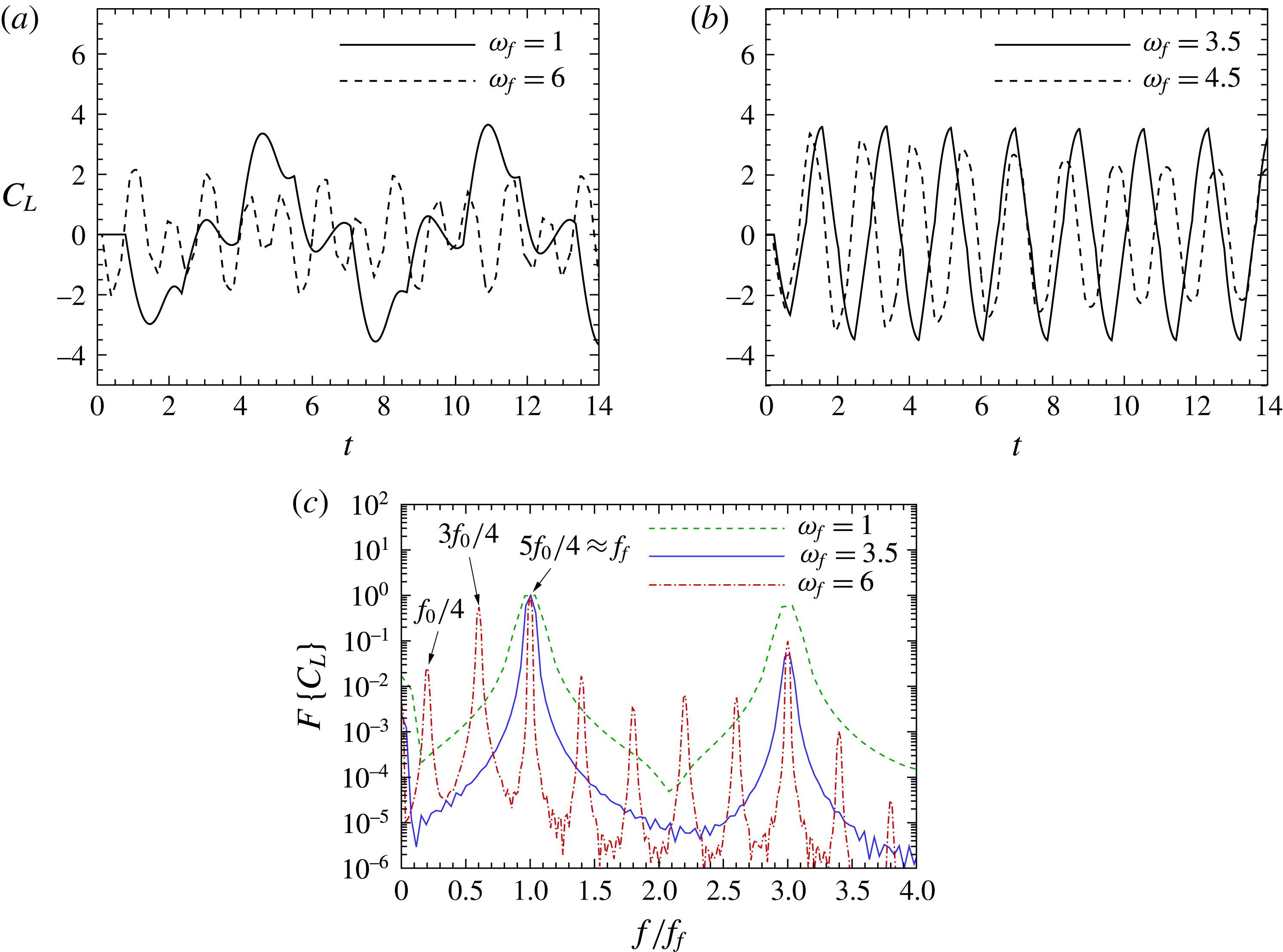
Figure 11. A typical time variation of the cylinder lift coefficient for
 $I=12$
and
$I=12$
and
 ${\it\omega}_{f}$
as indicated within (a) unlock-in regimes and (b) lock-in regimes. (c) Respective Fourier spectra of the lift coefficient signals in (a) and (b).
${\it\omega}_{f}$
as indicated within (a) unlock-in regimes and (b) lock-in regimes. (c) Respective Fourier spectra of the lift coefficient signals in (a) and (b).
The wake response was further assessed via spectral analysis of the vorticity time series recorded at the duct centreline and at different streamwise positions (five, ten and fifteen diameters downstream of the cylinder, corresponding to
 $x=2$
,
$x=2$
,
 $4$
and
$4$
and
 $6$
, respectively). It was found that, irrespective of the position where the signal was acquired, the wake exhibits a similar response (i.e. the spectrum peak is located at the same dominant frequency) for a given forcing amplitude and frequency. It was also observed that these signals have a similar response to the cylinder lift coefficient, except in the lock-in regime, where the frequency spectra exhibit peaks at odd harmonics. The appearance of these odd harmonic peaks in the spectrum is due to the absence of vorticity between two consecutive vortices of opposite sign, which results in an imperfect sinusoidal but symmetric waveform of vorticity time series (as shown in figure 12). For comparison, the corresponding cylinder lift coefficient time histories are shown in figure 11(b).
$6$
, respectively). It was found that, irrespective of the position where the signal was acquired, the wake exhibits a similar response (i.e. the spectrum peak is located at the same dominant frequency) for a given forcing amplitude and frequency. It was also observed that these signals have a similar response to the cylinder lift coefficient, except in the lock-in regime, where the frequency spectra exhibit peaks at odd harmonics. The appearance of these odd harmonic peaks in the spectrum is due to the absence of vorticity between two consecutive vortices of opposite sign, which results in an imperfect sinusoidal but symmetric waveform of vorticity time series (as shown in figure 12). For comparison, the corresponding cylinder lift coefficient time histories are shown in figure 11(b).

Figure 12. Time history of vorticity signal taken at
 $(x,y)=(0,5d)$
for
$(x,y)=(0,5d)$
for
 $I=12$
and
$I=12$
and
 ${\it\omega}_{f}$
as indicated.
${\it\omega}_{f}$
as indicated.
3.3 Effects of the current injection amplitude and gap ratio on heat transfer
This section examines the variation of HR with various forcing amplitude and at different transverse cylinder position. A typical plot is shown in figure 13. In general, HR increases with increasing forcing amplitude, with
 $\text{HR}_{max}\approx 1.9$
across the computed parameters. The increment is relatively substantial compared to the gain observed for oscillating cylinder cases, e.g. in Hussam et al. (Reference Hussam, Thompson and Sheard2012a
), where
$\text{HR}_{max}\approx 1.9$
across the computed parameters. The increment is relatively substantial compared to the gain observed for oscillating cylinder cases, e.g. in Hussam et al. (Reference Hussam, Thompson and Sheard2012a
), where
 $\text{HR}_{max}\approx 1.2$
was reported for a case with maximum oscillation amplitude (i.e.
$\text{HR}_{max}\approx 1.2$
was reported for a case with maximum oscillation amplitude (i.e.
 $A=3$
), at optimum frequency,
$A=3$
), at optimum frequency,
 $Re_{L}\approx 1800$
and
$Re_{L}\approx 1800$
and
 $H\approx 210$
. It is noted that at a lower range of
$H\approx 210$
. It is noted that at a lower range of
 $I$
(i.e.
$I$
(i.e.
 $I\lesssim 30$
), the forcing current injection has a more profound effect on the heat transfer enhancement when the cylinder is placed closest to the heated side of the duct wall (i.e.
$I\lesssim 30$
), the forcing current injection has a more profound effect on the heat transfer enhancement when the cylinder is placed closest to the heated side of the duct wall (i.e.
 $G/d=0.5$
) as compared to the other positions investigated. The reason for this is that when the cylinder is placed close to the wall, the shed vortices interact strongly with the thermal boundary layer in the vicinity of the cylinder, reducing its thickness and therefore increasing the local Nusselt number abruptly within the formation region (as shown by the sharp peak of the time-averaged local Nusselt number for the case of
$G/d=0.5$
) as compared to the other positions investigated. The reason for this is that when the cylinder is placed close to the wall, the shed vortices interact strongly with the thermal boundary layer in the vicinity of the cylinder, reducing its thickness and therefore increasing the local Nusselt number abruptly within the formation region (as shown by the sharp peak of the time-averaged local Nusselt number for the case of
 $G/d=0.5$
and
$G/d=0.5$
and
 $I=18$
in figure 14
a). On the other hand, the interaction between the wake and the thermal boundary layer becomes weaker as the cylinder is placed further away from the wall, which results in relatively lower HR and more consistent local
$I=18$
in figure 14
a). On the other hand, the interaction between the wake and the thermal boundary layer becomes weaker as the cylinder is placed further away from the wall, which results in relatively lower HR and more consistent local
 $Nu$
along the duct (as shown by the almost uniform local
$Nu$
along the duct (as shown by the almost uniform local
 $Nu$
profile for the case of
$Nu$
profile for the case of
 $G/d=2$
and
$G/d=2$
and
 $I=18$
in figure 14
a).
$I=18$
in figure 14
a).

Figure 13. Heat transfer enhancement ratio plotted against current injection amplitude
 $I$
at gap ratios
$I$
at gap ratios
 $G/d$
as indicated for
$G/d$
as indicated for
 $H=500$
,
$H=500$
,
 ${\it\tau}/T=0.25$
and
${\it\tau}/T=0.25$
and
 ${\it\omega}_{f}=1.75$
. The current is injected from the cylinder.
${\it\omega}_{f}=1.75$
. The current is injected from the cylinder.
However, for a large forcing amplitude, the duct with a cylinder placed on the centreline exhibits the highest enhancement in heat transfer. This occurs because for increasing
 $I$
, the vortex becomes larger (as seen in figure 15
a–c) and there is a consistently strong interaction between the heated wall and the cylinder wake along the duct. Furthermore, the local
$I$
, the vortex becomes larger (as seen in figure 15
a–c) and there is a consistently strong interaction between the heated wall and the cylinder wake along the duct. Furthermore, the local
 $Nu$
is progressively increased over a downstream region up to
$Nu$
is progressively increased over a downstream region up to
 $I=54$
(as shown in figure 14
b). Beyond
$I=54$
(as shown in figure 14
b). Beyond
 $I=54$
, the local
$I=54$
, the local
 $Nu$
exhibits a wavy pattern due to the complex interactions between the wake vortices and the thermal boundary layer (as shown in figure 15
b). Nevertheless,
$Nu$
exhibits a wavy pattern due to the complex interactions between the wake vortices and the thermal boundary layer (as shown in figure 15
b). Nevertheless,
 $Nu$
increases steadily with
$Nu$
increases steadily with
 $I$
, as shown by the almost linear trend in the
$I$
, as shown by the almost linear trend in the
 $\text{HR}$
–
$\text{HR}$
–
 $I$
plot. For the asymmetric cases, on the other hand, the strong wake–boundary layer interaction remains only in the vicinity of the cylinder even for high
$I$
plot. For the asymmetric cases, on the other hand, the strong wake–boundary layer interaction remains only in the vicinity of the cylinder even for high
 $I$
, which spans only approximately
$I$
, which spans only approximately
 $20\,\%$
of the duct length, whereby a rapid decrease in local
$20\,\%$
of the duct length, whereby a rapid decrease in local
 $Nu$
downstream of the local maxima was observed (as shown in figure 14(a) for cases with
$Nu$
downstream of the local maxima was observed (as shown in figure 14(a) for cases with
 $I=84$
). The reason for this observation is that the paired vortices are deflected away from the heated wall toward the opposite wall as they advect downstream (as shown in figure 15
d).
$I=84$
). The reason for this observation is that the paired vortices are deflected away from the heated wall toward the opposite wall as they advect downstream (as shown in figure 15
d).

Figure 14. Normalized time-averaged local Nusselt number along the downstream of the heated wall for
 ${\it\tau}/T=0.25$
,
${\it\tau}/T=0.25$
,
 ${\it\omega}_{f}=1.75$
and (a)
${\it\omega}_{f}=1.75$
and (a)
 $I$
and
$I$
and
 $G/d$
as indicated, and (b)
$G/d$
as indicated, and (b)
 $G/d=2$
and
$G/d=2$
and
 $I$
as indicated.
$I$
as indicated.
Note also that the
 $\text{HR}$
for cases with
$\text{HR}$
for cases with
 $G/d=1$
tend to level off for
$G/d=1$
tend to level off for
 $54\lesssim I\lesssim 78$
. A similar tendency was also observed for
$54\lesssim I\lesssim 78$
. A similar tendency was also observed for
 $G/d=0.5$
cases, except that for
$G/d=0.5$
cases, except that for
 $I\geqslant 60$
, there is another relatively smaller peak of local Nusselt number downstream of the first one, as shown in figure 14(a) for
$I\geqslant 60$
, there is another relatively smaller peak of local Nusselt number downstream of the first one, as shown in figure 14(a) for
 $I=84$
. This second peak emerges due to the strong wall vorticity entrainment into the wake, induced by the paired vortices that have effectively shed (refer vorticity contours in figure 15
d), and is attributed to the increase of HR with increasing
$I=84$
. This second peak emerges due to the strong wall vorticity entrainment into the wake, induced by the paired vortices that have effectively shed (refer vorticity contours in figure 15
d), and is attributed to the increase of HR with increasing
 $I$
at a high forcing amplitude range. A similar observation was reported for transversely (Celik et al.
Reference Celik, Raisee and Beskok2010) and rotationally (Beskok et al.
Reference Beskok, Raisee, Celik, Yagiz and Cheraghi2012) oscillating cylinders in duct arrangements, whereby the second peak of a local wall Nusselt number has a significant contribution to the spatial averaged heat transfer. It was also observed that as
$I$
at a high forcing amplitude range. A similar observation was reported for transversely (Celik et al.
Reference Celik, Raisee and Beskok2010) and rotationally (Beskok et al.
Reference Beskok, Raisee, Celik, Yagiz and Cheraghi2012) oscillating cylinders in duct arrangements, whereby the second peak of a local wall Nusselt number has a significant contribution to the spatial averaged heat transfer. It was also observed that as
 $I$
increases, the magnitude of the second peak was increased and its distance from the cylinder was decreased.
$I$
increases, the magnitude of the second peak was increased and its distance from the cylinder was decreased.

Figure 15. Instantaneous vorticity contour plots for (a)
 $I=30$
and
$I=30$
and
 $G/d=2$
, (c)
$G/d=2$
, (c)
 $I=54$
and
$I=54$
and
 $G/d=2$
, (b)
$G/d=2$
, (b)
 $I=78$
and
$I=78$
and
 $G/d=2$
and (d)
$G/d=2$
and (d)
 $I=84$
and
$I=84$
and
 $G/d=0.5$
.Contour levels are as per figure 5.
$G/d=0.5$
.Contour levels are as per figure 5.
3.4 Effects of the current injection pulse width and frequency on heat transfer
Here the variation of Nusselt number with different forcing pulse width and frequency is examined. Figure 16 reveals that the heat transfer enhancement ratio increases monotonically with increasing forcing pulse width. This may be explained as for a given forcing frequency, the wake vortex size is larger for a longer forcing pulse width (as shown in figure 17). As a result, the wake–boundary layer interaction is enhanced, thinning the thermal boundary layer at the heated wall and thus improving the convective heat transport.

Figure 16. Heat transfer enhancement ratio plotted against current injection pulse width
 ${\it\tau}/T$
at frequencies
${\it\tau}/T$
at frequencies
 ${\it\omega}_{f}$
as indicated for
${\it\omega}_{f}$
as indicated for
 $H=500$
,
$H=500$
,
 $I=30$
and
$I=30$
and
 $G/d=2$
. The current is injected from the cylinder.
$G/d=2$
. The current is injected from the cylinder.
Furthermore, cases with
 ${\it\omega}_{f}=1.75$
show a better heat transfer enhancement than the cases with
${\it\omega}_{f}=1.75$
show a better heat transfer enhancement than the cases with
 ${\it\omega}_{f}=3.5$
. This observation is in agreement with the findings presented in § 3.2, where the Nusselt number reaches its maximum value at
${\it\omega}_{f}=3.5$
. This observation is in agreement with the findings presented in § 3.2, where the Nusselt number reaches its maximum value at
 $1\lesssim {\it\omega}_{f}\lesssim 2$
for
$1\lesssim {\it\omega}_{f}\lesssim 2$
for
 $I=30$
. However, at the lowest forcing pulse width (i.e.
$I=30$
. However, at the lowest forcing pulse width (i.e.
 ${\it\tau}/T=0.05$
), the enhancement in heat transfer is almost similar for both forcing frequencies. This is due to the fact that for low
${\it\tau}/T=0.05$
), the enhancement in heat transfer is almost similar for both forcing frequencies. This is due to the fact that for low
 ${\it\tau}/T$
, the resultant wake vortices are relatively small, regardless of the forcing frequency. This in turn results in almost no interaction between the wake and the boundary layer (as shown in figure 17 for
${\it\tau}/T$
, the resultant wake vortices are relatively small, regardless of the forcing frequency. This in turn results in almost no interaction between the wake and the boundary layer (as shown in figure 17 for
 ${\it\tau}/T=0.05$
), which results in only an approximately 6 % enhancement in heat transfer.
${\it\tau}/T=0.05$
), which results in only an approximately 6 % enhancement in heat transfer.

Figure 17. Instantaneous vorticity contour plots for
 $I=30$
and (a)
$I=30$
and (a)
 ${\it\omega}_{f}=1.75$
and (b)
${\it\omega}_{f}=1.75$
and (b)
 ${\it\omega}_{f}=3.5$
. Contour levels are as per figure 5. (a,c)
${\it\omega}_{f}=3.5$
. Contour levels are as per figure 5. (a,c)
 ${\it\tau}/T=0.05$
, (b,d) 0.5.
${\it\tau}/T=0.05$
, (b,d) 0.5.
For cases with
 ${\it\tau}/T=0.5$
, although the forcing current injection is in the form of a square wave (as shown in figure 2), the resulting wake resembles that of a Kármán vortex shedding, where there is a finite spacing between two consecutive shed vortices of opposite sign. This may be understood as follows: as the vortex rolls up, it is advected downstream and is effectively ‘shed’ before the forcing current switches to the opposite sign, forming a long tail that connects to the succeeding shed vortex of opposite sign (as can be seen in figure 17
b,d). From these figures, it was also observed that the tail of the counter-clockwise (positive) vortices have a greater influence on thinning the thermal boundary layer than do the clockwise vortices. It is therefore anticipated that for a given pulse duty cycle
${\it\tau}/T=0.5$
, although the forcing current injection is in the form of a square wave (as shown in figure 2), the resulting wake resembles that of a Kármán vortex shedding, where there is a finite spacing between two consecutive shed vortices of opposite sign. This may be understood as follows: as the vortex rolls up, it is advected downstream and is effectively ‘shed’ before the forcing current switches to the opposite sign, forming a long tail that connects to the succeeding shed vortex of opposite sign (as can be seen in figure 17
b,d). From these figures, it was also observed that the tail of the counter-clockwise (positive) vortices have a greater influence on thinning the thermal boundary layer than do the clockwise vortices. It is therefore anticipated that for a given pulse duty cycle
 $D$
, the efficiency index may be further increased by injecting current which produces positive vorticity that has a longer pulse width relative to the negative vorticity. Here,
$D$
, the efficiency index may be further increased by injecting current which produces positive vorticity that has a longer pulse width relative to the negative vorticity. Here,
 $D=2{\it\tau}/T$
for a modified square wave, which represents a fraction of one period in which the signal is active. This would be an interesting avenue for future study.
$D=2{\it\tau}/T$
for a modified square wave, which represents a fraction of one period in which the signal is active. This would be an interesting avenue for future study.
3.5 Effects of the electrode position relative to the cylinder on heat transfer
The effect of electrode position on the heat transfer enhancement ratio is demonstrated in figure 18. The electrode was placed at 18 different positions in the vicinity of the cylinder and the heated wall, in order to investigate the effect of complex interactions between the shear layers on the global heat transfer. Other parameters are fixed at
 $H=500$
,
$H=500$
,
 $I=12$
,
$I=12$
,
 ${\it\omega}_{f}=1.75$
,
${\it\omega}_{f}=1.75$
,
 ${\it\tau}/T=0.25$
and
${\it\tau}/T=0.25$
and
 $G/d=2$
. The figure reveals that the enhancement in heat transfer is almost independent of the streamwise electrode position. The reason for this observation is due to the counterbalancing effect of the relative ‘surplus’ and ‘deficit’ in the local
$G/d=2$
. The figure reveals that the enhancement in heat transfer is almost independent of the streamwise electrode position. The reason for this observation is due to the counterbalancing effect of the relative ‘surplus’ and ‘deficit’ in the local
 $Nu$
(as depicted by the shaded regions in figure 19
a); increased heat transfer downstream of the electrode as it is placed further downstream is offset by the larger region upstream of the electrode exhibiting low heat transfer. This happens because the heat transfer enhancement was observed to occur only at the downstream of the electrode (i.e. there was almost no enhancement at
$Nu$
(as depicted by the shaded regions in figure 19
a); increased heat transfer downstream of the electrode as it is placed further downstream is offset by the larger region upstream of the electrode exhibiting low heat transfer. This happens because the heat transfer enhancement was observed to occur only at the downstream of the electrode (i.e. there was almost no enhancement at
 $x\lesssim l_{x}$
), and due to the variations in the magnitude and/or location of the local
$x\lesssim l_{x}$
), and due to the variations in the magnitude and/or location of the local
 $Nu$
peaks with
$Nu$
peaks with
 $l_{x}$
.
$l_{x}$
.

Figure 18. Heat transfer enhancement ratio plotted against horizontal distance
 $l_{x}$
at vertical distance
$l_{x}$
at vertical distance
 $l_{y}$
as indicated for
$l_{y}$
as indicated for
 $I=12$
,
$I=12$
,
 ${\it\omega}_{f}=1.75$
,
${\it\omega}_{f}=1.75$
,
 ${\it\tau}/T=0.25$
and
${\it\tau}/T=0.25$
and
 $G/d=2$
.
$G/d=2$
.
Figure 18 also reveals that the heat transfer is significantly more sensitive to transverse electrode position. Inspection of the normalized local Nusselt number reveals that, for a given
 $l_{x}$
, the peaks for cases with
$l_{x}$
, the peaks for cases with
 $l_{y}=0.4$
are consistently higher than for the cases with
$l_{y}=0.4$
are consistently higher than for the cases with
 $l_{y}=0.6$
(as shown in figure 19
b). The magnitude, however, decreased abruptly downstream of the electrode, due to the aforementioned deflection of shed vortices away from the heated wall toward the opposite wall for the offset cylinder cases. This leads to a lower overall heat transfer enhancement than for cases with electrode placed at
$l_{y}=0.6$
(as shown in figure 19
b). The magnitude, however, decreased abruptly downstream of the electrode, due to the aforementioned deflection of shed vortices away from the heated wall toward the opposite wall for the offset cylinder cases. This leads to a lower overall heat transfer enhancement than for cases with electrode placed at
 $l_{y}=0.6$
.
$l_{y}=0.6$
.

Figure 19. Normalized time-averaged local Nusselt number along the downstream of the heated wall. (a) The electrode is placed at
 $l_{y}=0.6$
and at
$l_{y}=0.6$
and at
 $l_{x}$
as indicated. The dark (lighter) region correspond to a deficit (surplus) in heat transfer enhancement of case with
$l_{x}$
as indicated. The dark (lighter) region correspond to a deficit (surplus) in heat transfer enhancement of case with
 $l_{x}=2$
relative to the case with
$l_{x}=2$
relative to the case with
 $l_{x}=0.4$
. (b) The electrode is placed at
$l_{x}=0.4$
. (b) The electrode is placed at
 $l_{x}=2$
and at
$l_{x}=2$
and at
 $l_{y}$
as indicated.
$l_{y}$
as indicated.
For a given
 $l_{y}$
, the magnitude of the peaks were almost invariant with respect to
$l_{y}$
, the magnitude of the peaks were almost invariant with respect to
 $l_{x}$
(with the coefficient of variation,
$l_{x}$
(with the coefficient of variation,
 $0.015\leqslant CV\leqslant 0.046$
for all
$0.015\leqslant CV\leqslant 0.046$
for all
 $l_{x}$
), indicating that the magnitude of the peaks is governed by the electrode–wall proximity. However, at
$l_{x}$
), indicating that the magnitude of the peaks is governed by the electrode–wall proximity. However, at
 $l_{y}=0.6$
, the peak of time-averaged
$l_{y}=0.6$
, the peak of time-averaged
 $Nu_{x}/Nu_{x,0}$
for
$Nu_{x}/Nu_{x,0}$
for
 $l_{x}=0$
is significantly lower than the peaks for other
$l_{x}=0$
is significantly lower than the peaks for other
 $l_{x}$
(as can be seen in figure 19
a), which results in
$l_{x}$
(as can be seen in figure 19
a), which results in
 $\text{HR}$
lower than the case for
$\text{HR}$
lower than the case for
 $l_{y}=0.4$
for the same
$l_{y}=0.4$
for the same
 $l_{x}$
(as shown in figure 18). This observation is consistent with the results presented in figure 13, where at a lower range of
$l_{x}$
(as shown in figure 18). This observation is consistent with the results presented in figure 13, where at a lower range of
 $I$
,
$I$
,
 $\text{HR}$
is higher when the cylinder is placed closest to the heated wall.
$\text{HR}$
is higher when the cylinder is placed closest to the heated wall.
For the cases with electrode placed at the duct centreline, the wake–boundary layer interaction is weak throughout the duct, and there were no strong peaks observed in the local
 $Nu$
-
$Nu$
-
 $x$
plot. The peaks are consistently lower than for the offset electrode counterparts, which leads to a lower
$x$
plot. The peaks are consistently lower than for the offset electrode counterparts, which leads to a lower
 $\text{HR}$
for any given
$\text{HR}$
for any given
 $l_{x}$
.
$l_{x}$
.
3.6 Effects of friction parameter and Reynolds number on heat transfer
This section reports the influence of magnetic field strength (quantified by friction parameter
 $H$
) and Reynolds number. Other parameters are fixed at
$H$
) and Reynolds number. Other parameters are fixed at
 $I=30$
,
$I=30$
,
 ${\it\omega}_{f}=1.75$
,
${\it\omega}_{f}=1.75$
,
 ${\it\tau}/T=0.25$
,
${\it\tau}/T=0.25$
,
 $G/d=2$
. The results are shown in figure 20 for
$G/d=2$
. The results are shown in figure 20 for
 $200\leqslant H\leqslant 5000$
and
$200\leqslant H\leqslant 5000$
and
 $Re_{L}=1500$
and
$Re_{L}=1500$
and
 $3000$
. The figure shows that for a given Reynolds number, the enhancement in heat transfer due to the imposed current exhibits a non-monotonic relation with friction parameter. At low
$3000$
. The figure shows that for a given Reynolds number, the enhancement in heat transfer due to the imposed current exhibits a non-monotonic relation with friction parameter. At low
 $H$
,
$H$
,
 $\text{HR}$
increases with increasing
$\text{HR}$
increases with increasing
 $H$
and reaches a peak, before decreasing steadily with further increases in
$H$
and reaches a peak, before decreasing steadily with further increases in
 $H$
and eventually reaching an asymptotic value.
$H$
and eventually reaching an asymptotic value.

Figure 20. (Primary vertical axis) heat transfer enhancement ratio and (secondary vertical axis) base flows time-averaged Nusselt number plotted against friction parameter
 $H$
for Reynolds numbers
$H$
for Reynolds numbers
 $Re_{L}=1500$
and
$Re_{L}=1500$
and
 $3000$
. Open symbols represent HR and solid symbols represent
$3000$
. Open symbols represent HR and solid symbols represent
 $Nu_{0}$
. The dashed lines indicate a critical value of the friction parameter, above which the cylinder vortex shedding is completely suppressed.
$Nu_{0}$
. The dashed lines indicate a critical value of the friction parameter, above which the cylinder vortex shedding is completely suppressed.

Figure 21. (a,b) Instantaneous vorticity contour plots for
 $Re_{L}=1500$
and (a)
$Re_{L}=1500$
and (a)
 $H=300$
and (b)
$H=300$
and (b)
 $H=1500$
. Contour levels are as per figure 5. (c) Normalized time-averaged local Nusselt number along the downstream of the heated wall for
$H=1500$
. Contour levels are as per figure 5. (c) Normalized time-averaged local Nusselt number along the downstream of the heated wall for
 $Re_{L}=1500$
and
$Re_{L}=1500$
and
 $H$
as indicated.
$H$
as indicated.
This observation is attributed to the competition between inertia and Hartmann damping, i.e.
 $(a^{2}/nL^{2})Re_{L}/Ha$
(Sommeria Reference Sommeria1986). In the low-
$(a^{2}/nL^{2})Re_{L}/Ha$
(Sommeria Reference Sommeria1986). In the low-
 $H$
regime, the inertially shed and electrically driven vortices dominate over the damping force, which results in shed vortices being sustained to greater downstream distances. There is a consistently strong interaction between the heated wall and the cylinder wake along the duct, visible in the vorticity field plot in figure 21(a). Consequently, the enhancement in the local Nusselt number is nearly uniform throughout the domain (as shown by the almost horizontal curve for
$H$
regime, the inertially shed and electrically driven vortices dominate over the damping force, which results in shed vortices being sustained to greater downstream distances. There is a consistently strong interaction between the heated wall and the cylinder wake along the duct, visible in the vorticity field plot in figure 21(a). Consequently, the enhancement in the local Nusselt number is nearly uniform throughout the domain (as shown by the almost horizontal curve for
 $H=200$
in figure 21
c). In the high-
$H=200$
in figure 21
c). In the high-
 $H$
regime, however, Hartmann damping dominates over the driving force. The strength of the shed vortices is relatively high in the near wake due to the strong interaction between the magnetic field and the imposed current forcing, but is damped rapidly after they are shed (as indicated in the plot of vorticity contour in figure 21
b). As a result, the strong wake–boundary layer interaction occurs only in the near-wake region, which is reflected by the strong peak of local Nusselt number in the vicinity of the cylinder, followed by a rapid decline further downstream (as shown in figure 21(b) for friction parameters in the high-
$H$
regime, however, Hartmann damping dominates over the driving force. The strength of the shed vortices is relatively high in the near wake due to the strong interaction between the magnetic field and the imposed current forcing, but is damped rapidly after they are shed (as indicated in the plot of vorticity contour in figure 21
b). As a result, the strong wake–boundary layer interaction occurs only in the near-wake region, which is reflected by the strong peak of local Nusselt number in the vicinity of the cylinder, followed by a rapid decline further downstream (as shown in figure 21(b) for friction parameters in the high-
 $H$
regime). With
$H$
regime). With
 $H$
increasing further, the flow field is dominated by the forcing current. However, due to very strong damping, the shedding is completely suppressed and the heat transfer eventually becomes asymptotically independent of
$H$
increasing further, the flow field is dominated by the forcing current. However, due to very strong damping, the shedding is completely suppressed and the heat transfer eventually becomes asymptotically independent of
 $H$
.
$H$
.
 $\text{HR}$
reaches its maximum value at a friction parameter close to the critical value
$\text{HR}$
reaches its maximum value at a friction parameter close to the critical value
 $H_{c}$
at which a transition between time-dependent and steady state flows occurs in the base flows. The Nusselt number for the base flows, however, reaches an asymptote beyond the critical friction parameter due to laminarisation (as can be seen in figure 20). This observation is in contrast to cases where the duct walls are conducting, where
$H_{c}$
at which a transition between time-dependent and steady state flows occurs in the base flows. The Nusselt number for the base flows, however, reaches an asymptote beyond the critical friction parameter due to laminarisation (as can be seen in figure 20). This observation is in contrast to cases where the duct walls are conducting, where
 $Nu$
increased with increasing
$Nu$
increased with increasing
 $Ha$
due to high velocity gradient near the heated wall (Cuevas et al.
Reference Cuevas, Picologlou, Walker, Talmage and Hua1997; Takahashi et al.
Reference Takahashi, Aritomi, Inoue and Matsuzaki1998). Furthermore, the flow with higher
$Ha$
due to high velocity gradient near the heated wall (Cuevas et al.
Reference Cuevas, Picologlou, Walker, Talmage and Hua1997; Takahashi et al.
Reference Takahashi, Aritomi, Inoue and Matsuzaki1998). Furthermore, the flow with higher
 $Re_{L}$
reached a higher asymptote in the steady state regime due to the increased level of turbulence, which is favourable for effective heat dissipation (Sukoriansky et al.
Reference Sukoriansky, Klaiman, Branover and Greenspan1989). The value of
$Re_{L}$
reached a higher asymptote in the steady state regime due to the increased level of turbulence, which is favourable for effective heat dissipation (Sukoriansky et al.
Reference Sukoriansky, Klaiman, Branover and Greenspan1989). The value of
 $H_{c}$
was refined by means of a Stuart–Landau analysis, which while primarily being a tool for analysing the nonlinear futures of an evolving instability, is also convenient for recovering the exponential growth or decay rate for an instability in its linear regime (further details concerning this analysis technique can be found in Hussam, Thompson & Sheard (Reference Hussam, Thompson and Sheard2011)). Noting the Hartmann friction term in (2.4), the heat transfer enhancement ratio is plotted against
$H_{c}$
was refined by means of a Stuart–Landau analysis, which while primarily being a tool for analysing the nonlinear futures of an evolving instability, is also convenient for recovering the exponential growth or decay rate for an instability in its linear regime (further details concerning this analysis technique can be found in Hussam, Thompson & Sheard (Reference Hussam, Thompson and Sheard2011)). Noting the Hartmann friction term in (2.4), the heat transfer enhancement ratio is plotted against
 $H/Re_{L}$
, as shown in figure 22. The figure shows that the
$H/Re_{L}$
, as shown in figure 22. The figure shows that the
 $\text{HR}$
data for both Reynolds numbers nearly collapses into a single curve, suggesting that the enhancement of heat transfer is governed by the
$\text{HR}$
data for both Reynolds numbers nearly collapses into a single curve, suggesting that the enhancement of heat transfer is governed by the
 $H/Re_{L}$
. This observation is perhaps not surprising, given that the stability (Sommeria Reference Sommeria1986) and the decay of vortices (Sommeria Reference Sommeria1988; Hamid et al.
Reference Hamid, Hussam, Pothérat and Sheard2015) in quasi-two-dimensional MHD duct flows are controlled by the
$H/Re_{L}$
. This observation is perhaps not surprising, given that the stability (Sommeria Reference Sommeria1986) and the decay of vortices (Sommeria Reference Sommeria1988; Hamid et al.
Reference Hamid, Hussam, Pothérat and Sheard2015) in quasi-two-dimensional MHD duct flows are controlled by the
 $H/Re_{L}$
parameter.
$H/Re_{L}$
parameter.

Figure 22. Heat transfer enhancement ratio and plotted against
 $H/Re_{L}$
for
$H/Re_{L}$
for
 $Re_{L}$
as indicated. Circle and delta symbols represent
$Re_{L}$
as indicated. Circle and delta symbols represent
 $Re_{L}=1500$
and
$Re_{L}=1500$
and
 $3000$
, respectively.
$3000$
, respectively.
4 Power and efficiency analysis
In this section, the characteristics of pumping power requirement (expressed in terms of pressure penalty ratio), overall system efficiency resulting from the employment of current injection as a turbulence enhancer and the current injection power input are reported. The pressure penalty ratio
 $\text{PR}$
in this study is the ratio of pressure drop across identical ducts with and without current injection. Inspection of
$\text{PR}$
in this study is the ratio of pressure drop across identical ducts with and without current injection. Inspection of
 $\text{PR}$
across all cases in this study (not shown for brevity) reveals that the pressure drop induced by the imposed current injection is almost negligible, with the maximum pressure increment of
$\text{PR}$
across all cases in this study (not shown for brevity) reveals that the pressure drop induced by the imposed current injection is almost negligible, with the maximum pressure increment of
 $13\,\%$
(i.e.
$13\,\%$
(i.e.
 $\text{PR}_{max}=1.13$
). It was also observed that the position of the electrode and magnetic field strength have almost no effect on
$\text{PR}_{max}=1.13$
). It was also observed that the position of the electrode and magnetic field strength have almost no effect on
 $\text{PR}$
, where the mean (and standard deviation in parentheses) of
$\text{PR}$
, where the mean (and standard deviation in parentheses) of
 $\text{PR}$
for various investigated electrode positions and Hartmann numbers are respectively 1.004 (0.0032) and 1.012 (0.0067). Furthermore, it was found that cases with the cylinder at the duct centreline show a relatively higher increment in pressure drop as compared to the cases with an offset cylinder, and becomes more apparent at a higher current amplitude. In some cases, the imposed current injection has a desirable effect by reducing the pressure drop with respect to the base cases, with a maximum reduction of
$\text{PR}$
for various investigated electrode positions and Hartmann numbers are respectively 1.004 (0.0032) and 1.012 (0.0067). Furthermore, it was found that cases with the cylinder at the duct centreline show a relatively higher increment in pressure drop as compared to the cases with an offset cylinder, and becomes more apparent at a higher current amplitude. In some cases, the imposed current injection has a desirable effect by reducing the pressure drop with respect to the base cases, with a maximum reduction of
 $4\,\%$
(i.e.
$4\,\%$
(i.e.
 $\text{PR}_{min}=0.96$
). Since
$\text{PR}_{min}=0.96$
). Since
 $\text{PR}$
is almost unity for all cases, it follows then that the system efficiency (quantified by the efficiency index
$\text{PR}$
is almost unity for all cases, it follows then that the system efficiency (quantified by the efficiency index
 ${\it\eta}$
as in (2.11)) and the heat transfer enhancement ratio
${\it\eta}$
as in (2.11)) and the heat transfer enhancement ratio
 $\text{HR}$
have a similar dependency on all varying parameters (as presented in the previous sections). The maximum efficiency index was found to be
$\text{HR}$
have a similar dependency on all varying parameters (as presented in the previous sections). The maximum efficiency index was found to be
 ${\it\eta}=1.91$
for the case with highest current amplitude, which produces the highest heat transfer enhancement ratio of
${\it\eta}=1.91$
for the case with highest current amplitude, which produces the highest heat transfer enhancement ratio of
 $\text{HR}=1.89$
. This enhancement in heat transfer is 55 % more than what has been reported for rotationally oscillating cylinder rotating at maximum amplitude and optimum frequency (i.e.
$\text{HR}=1.89$
. This enhancement in heat transfer is 55 % more than what has been reported for rotationally oscillating cylinder rotating at maximum amplitude and optimum frequency (i.e.
 $\text{HR}\approx 1.22$
) (Hussam et al.
Reference Hussam, Thompson and Sheard2012a
). In the hydrodynamic counterpart, maximum enhancement of
$\text{HR}\approx 1.22$
) (Hussam et al.
Reference Hussam, Thompson and Sheard2012a
). In the hydrodynamic counterpart, maximum enhancement of
 $\text{HR}\approx 1.55$
has been reported when the cylinder with
$\text{HR}\approx 1.55$
has been reported when the cylinder with
 ${\it\beta}=1/3$
rotationally oscillates with maximum amplitude and within the lock-in regime (Beskok et al.
Reference Beskok, Raisee, Celik, Yagiz and Cheraghi2012).
${\it\beta}=1/3$
rotationally oscillates with maximum amplitude and within the lock-in regime (Beskok et al.
Reference Beskok, Raisee, Celik, Yagiz and Cheraghi2012).
It is important to mention that the effect of inertially driven recirculation in the parallel planes on the heat transfer is assumed to be negligible in the present work. Recent investigation by Baker, Pothérat & Davoust (Reference Baker, Pothérat and Davoust2015) has shown that in the limit of quasi-2-D base flow, the local fluid rotation above the Hartmann layer induces secondary counter-rotating 3-D recirculations which correspond to Ekman pumping. The emergence of these recirculations drives an inward radial flow within the Hartmann layers, and thus can potentially transport a fraction of heat towards the core flow and alter the heat transfer characteristics of the flow. However, it has been reported (Alboussière, Uspenski & Moreau Reference Alboussière, Uspenski and Moreau1999) that the 3-D recirculation is weakened under a strong magnetic field. It is then anticipated that this weak recirculation becomes less effective in transferring heat relative to the primary vortex flow, justifying the aforementioned assumption.
The average power supply due to current injection is proportional to
 $I_{rms}^{2}$
, where
$I_{rms}^{2}$
, where
 $I_{rms}$
is the root mean square of injected current. Since the dimensional current amplitude
$I_{rms}$
is the root mean square of injected current. Since the dimensional current amplitude
 $$\begin{eqnarray}\displaystyle \hat{I} =IaU_{0}\sqrt{{\it\rho}{\it\nu}{\it\sigma}}=2{\it\alpha}\sqrt{{\it\rho}{\it\nu}^{3}{\it\sigma}}IRe_{L}, & & \displaystyle\end{eqnarray}$$
and taking the properties of a low melting point eutectic alloy
 $\text{Ga}^{68}\text{In}^{20}\text{Sn}^{12}$
at
$\text{Ga}^{68}\text{In}^{20}\text{Sn}^{12}$
at
 $20\,^{\circ }\text{C}$
(as presented in § 2.2) and
$20\,^{\circ }\text{C}$
(as presented in § 2.2) and
 ${\it\alpha}=1$
, the dimensional current injection amplitude is given by
${\it\alpha}=1$
, the dimensional current injection amplitude is given by
 $$\begin{eqnarray}\displaystyle \hat{I} \approx 5.96\times 10^{-5}IRe_{L}\,\text{A}. & & \displaystyle\end{eqnarray}$$
In the present investigation, the bulk of the numerical simulations were based on the flow Reynolds number
 $Re_{L}=1500$
, while the dimensionless current injection amplitude was varied between 6 and 90, this then corresponds to a dimensional current of
$Re_{L}=1500$
, while the dimensionless current injection amplitude was varied between 6 and 90, this then corresponds to a dimensional current of
 $\hat{I} \approx 0.5$
and 8 A, respectively. For the sake of comparison, this current supply is three orders of magnitude lower than that required to induce the confining magnetic fields for fusion blanket MHD research in the MEKKA experimental facility (Barleon, Mack & Stieglitz Reference Barleon, Mack and Stieglitz1996). The use of electrically generated quasi-two-dimensional vortices for heat transfer augmentation therefore appears to be viable, at least in principle. There are, however, significant technical challenges in realizing controlled current injection through electrodes that are embedded in a Hartmann wall. These include ensuring good contact between the electrode surface and the liquid metal, as poor contact can lead to overheating, and the effect on the fluid rotation above the electrode may be significant. Furthermore, the electrode–liquid metal interface is also susceptible to varying resistance, where erratic variation in contact resistance can lead to an irregular electric current distribution over multiple electrodes. This effect can be avoided by incorporating ohmic resistance of orders of magnitudes higher than any other resistance in electric circuit of each electrode (Pothérat & Klein Reference Pothérat and Klein2014). This solution would, however, result in energy consumption significantly higher than previously estimated. Furthermore, it has been shown previously that the electrical resistance increases monotonically with increasing imposed magnetic field (Sommeria Reference Sommeria1988). The technological challenges toward implementation of such system are outside the scope of the present study.
$\hat{I} \approx 0.5$
and 8 A, respectively. For the sake of comparison, this current supply is three orders of magnitude lower than that required to induce the confining magnetic fields for fusion blanket MHD research in the MEKKA experimental facility (Barleon, Mack & Stieglitz Reference Barleon, Mack and Stieglitz1996). The use of electrically generated quasi-two-dimensional vortices for heat transfer augmentation therefore appears to be viable, at least in principle. There are, however, significant technical challenges in realizing controlled current injection through electrodes that are embedded in a Hartmann wall. These include ensuring good contact between the electrode surface and the liquid metal, as poor contact can lead to overheating, and the effect on the fluid rotation above the electrode may be significant. Furthermore, the electrode–liquid metal interface is also susceptible to varying resistance, where erratic variation in contact resistance can lead to an irregular electric current distribution over multiple electrodes. This effect can be avoided by incorporating ohmic resistance of orders of magnitudes higher than any other resistance in electric circuit of each electrode (Pothérat & Klein Reference Pothérat and Klein2014). This solution would, however, result in energy consumption significantly higher than previously estimated. Furthermore, it has been shown previously that the electrical resistance increases monotonically with increasing imposed magnetic field (Sommeria Reference Sommeria1988). The technological challenges toward implementation of such system are outside the scope of the present study.
5 Conclusions
The present study has investigated the characteristics of electrically generated quasi-two-dimensional vortices to enhance sidewall heat transfer in MHD ducts containing a circular cylinder vortex promoter under a strong transverse magnetic field. A solution to the current injection forcing field was first derived for a domain extending infinitely in streamwise direction and bounded by duct sidewalls, and was imposed as a forcing field in simulations of the quasi-two-dimensional flows. It was found that the heat transfer enhancement are closely associated with the resulting wake dynamics and their interactions with the heated wall. The results indicate a maximum Nusselt number improvement of about
 $90\,\%$
for ducts with current injection, and is highly dependent on the imposed forcing current parameters. Non-monotonic relationships between the heat transfer enhancement ratio
$90\,\%$
for ducts with current injection, and is highly dependent on the imposed forcing current parameters. Non-monotonic relationships between the heat transfer enhancement ratio
 $\text{HR}$
and the forcing frequency and magnetic field strength were observed. The
$\text{HR}$
and the forcing frequency and magnetic field strength were observed. The
 $\text{HR}$
, however, increased almost linearly with forcing amplitude and pulse width. It is also significantly influenced by the electrode position in the transverse direction.
$\text{HR}$
, however, increased almost linearly with forcing amplitude and pulse width. It is also significantly influenced by the electrode position in the transverse direction.
An examination of the local Nusselt number variation along the duct revealed a general trend wherein a sudden jump were followed by an abrupt decrease in the local
 $Nu$
, due to the deflection of the wake vortices away from the heated wall. In some cases, the appearance of secondary peak in the local Nusselt number plots has a significant contribution to the overall heat transfer enhancement. Despite the different mechanism of vortex generation in the present MHD duct flow, the heat transfer enhancement exhibits similar characteristics to the hydrodynamic counterpart, whereby the local Nusselt number distribution is closely associated with the strength of the wake–boundary layer interaction and the entrainment of fluid from the boundary layer into the wake. The factors determining the interaction and entrainment are the size, pattern/mode and frequency of shedding of the wake vortex.
$Nu$
, due to the deflection of the wake vortices away from the heated wall. In some cases, the appearance of secondary peak in the local Nusselt number plots has a significant contribution to the overall heat transfer enhancement. Despite the different mechanism of vortex generation in the present MHD duct flow, the heat transfer enhancement exhibits similar characteristics to the hydrodynamic counterpart, whereby the local Nusselt number distribution is closely associated with the strength of the wake–boundary layer interaction and the entrainment of fluid from the boundary layer into the wake. The factors determining the interaction and entrainment are the size, pattern/mode and frequency of shedding of the wake vortex.
Spectral analysis of the cylinder lift coefficient revealed broadening of lock-in regime with increasing forcing amplitude. The analysis also revealed a distinct spectrum of cylinder lift coefficient in the unlock-in regime. Nonlinear coupling of the cylinder vortex shedding with the forcing current injection can account for distinct spectral peaks beyond the lock-in regime.
The analysis of the pressure drop indicates that the employment of current injection as turbuliser does not significantly alter the hydraulic losses. This yields an efficiency index ranging between
 $97\,\%$
and
$97\,\%$
and
 $191\,\%$
.
$191\,\%$
.
Acknowledgements
This research was supported by the Australian Research Council through Discovery grants DP120100153 and DP150102920, a high-performance computing time allocations from the National Computational Infrastructure (NCI), which is supported by the Australian Government, and the Monash SunGRID. The authors are grateful to Professor A. Pothérat, Coventry University, for helpful discussions and advice, and also thank the anonymous referees for their productive comments and suggestions. A.H.A.H. is supported by the Malaysia Ministry of Education and the Universiti Teknologi MARA, Malaysia.
Appendix A
In (2.4), the non-dimensional forcing velocity field
 $\boldsymbol{u}_{0}$
is defined as
$\boldsymbol{u}_{0}$
is defined as
 $$\begin{eqnarray}\displaystyle \boldsymbol{u}_{0}=\boldsymbol{j}\times \boldsymbol{e}_{z}=\boldsymbol{{\rm\nabla}}{\it\psi}_{0}\times \boldsymbol{e}_{z}, & & \displaystyle\end{eqnarray}$$
where
 $\boldsymbol{j}$
is the electric current density,
$\boldsymbol{j}$
is the electric current density,
 $\boldsymbol{e}_{z}$
is the unit vector in the
$\boldsymbol{e}_{z}$
is the unit vector in the
 $z$
-direction and
$z$
-direction and
 ${\it\psi}_{0}$
is the electrical potential. The electric current density and the electrical potential are scaled by
${\it\psi}_{0}$
is the electrical potential. The electric current density and the electrical potential are scaled by
 ${\it\sigma}BU_{0}/Ha=U_{0}\sqrt{{\it\rho}{\it\nu}{\it\sigma}}/a$
and
${\it\sigma}BU_{0}/Ha=U_{0}\sqrt{{\it\rho}{\it\nu}{\it\sigma}}/a$
and
 $aBU_{0}$
, respectively. In a high magnetic field application, the change in the field due to the currents induced by the flow can be neglected. Under this condition, the equations governing continuity of electric current and incompressibility are also linear, so they may be averaged to give
$aBU_{0}$
, respectively. In a high magnetic field application, the change in the field due to the currents induced by the flow can be neglected. Under this condition, the equations governing continuity of electric current and incompressibility are also linear, so they may be averaged to give
 $\boldsymbol{{\rm\nabla}}\boldsymbol{\cdot }\boldsymbol{j}=-j_{w}$
,
$\boldsymbol{{\rm\nabla}}\boldsymbol{\cdot }\boldsymbol{j}=-j_{w}$
,
 $\boldsymbol{j}=Ha(\boldsymbol{E}+\boldsymbol{u}\times \boldsymbol{e}_{z})$
and
$\boldsymbol{j}=Ha(\boldsymbol{E}+\boldsymbol{u}\times \boldsymbol{e}_{z})$
and
 $\boldsymbol{{\rm\nabla}}\boldsymbol{\cdot }\boldsymbol{u}=0$
. Here
$\boldsymbol{{\rm\nabla}}\boldsymbol{\cdot }\boldsymbol{u}=0$
. Here
 $j_{w}$
is the current density injected at one or both of the confining planes, and
$j_{w}$
is the current density injected at one or both of the confining planes, and
 $\boldsymbol{E}$
is a dimensionless electrical field. The
$\boldsymbol{E}$
is a dimensionless electrical field. The
 $z$
-averaged current can be expressed as the gradient of a scalar field
$z$
-averaged current can be expressed as the gradient of a scalar field
 ${\it\psi}_{0}$
satisfying a Poisson equation with the source term being
${\it\psi}_{0}$
satisfying a Poisson equation with the source term being
 $j_{w}$
, i.e.
$j_{w}$
, i.e.
 $\boldsymbol{j}=\boldsymbol{{\rm\nabla}}{\it\psi}_{0}$
, obtained from
$\boldsymbol{j}=\boldsymbol{{\rm\nabla}}{\it\psi}_{0}$
, obtained from
 ${\rm\nabla}^{2}{\it\psi}_{0}=-j_{w}$
(Pothérat et al.
Reference Pothérat, Sommeria and Moreau2005). This Poisson equation is first solved (Polyanin Reference Polyanin2001) for a source term at the current injection point that is a Dirac function located at
${\rm\nabla}^{2}{\it\psi}_{0}=-j_{w}$
(Pothérat et al.
Reference Pothérat, Sommeria and Moreau2005). This Poisson equation is first solved (Polyanin Reference Polyanin2001) for a source term at the current injection point that is a Dirac function located at
 $(0,l_{y})$
, i.e.
$(0,l_{y})$
, i.e.
 $j_{w}(x,y)=I{\it\delta}(x,y-l_{y})$
, on a domain extending infinitely in streamwise direction and bounded by duct sidewalls at
$j_{w}(x,y)=I{\it\delta}(x,y-l_{y})$
, on a domain extending infinitely in streamwise direction and bounded by duct sidewalls at
 $y=\pm 1$
. Physically, the current circuit would be completed far upstream and downstream of the electrode. Imposing zero Neumann conditions on the electrical potential field at the boundaries due to the insulating Shercliff walls (Pothérat et al.
Reference Pothérat, Sommeria and Moreau2000), i.e.
$y=\pm 1$
. Physically, the current circuit would be completed far upstream and downstream of the electrode. Imposing zero Neumann conditions on the electrical potential field at the boundaries due to the insulating Shercliff walls (Pothérat et al.
Reference Pothérat, Sommeria and Moreau2000), i.e.
 $\partial {\it\psi}_{0}/\partial y=0$
at
$\partial {\it\psi}_{0}/\partial y=0$
at
 $y=\pm 1$
, leads to
$y=\pm 1$
, leads to
 $$\begin{eqnarray}\displaystyle {\it\psi}_{0}(x,y) & = & \displaystyle \frac{I}{4{\rm\pi}}\left[\log \left(\frac{1}{\cosh ({\rm\pi}x/2)-\cos [{\rm\pi}(y+1+l_{y})/2]}\right)\right.\nonumber\\ \displaystyle & & \displaystyle \left.+\,\log \left(\frac{1}{\cosh ({\rm\pi}x/2)-\cos [{\rm\pi}(y+1-l_{y})/2]}\right)\right].\end{eqnarray}$$
 $I$
is the non-dimensional current amplitude, which is defined as
$I$
is the non-dimensional current amplitude, which is defined as
 $$\begin{eqnarray}\displaystyle I=\frac{\hat{I} }{aU_{0}\sqrt{{\it\rho}{\it\nu}{\it\sigma}}}. & & \displaystyle\end{eqnarray}$$
Substituting (A 2) into (A 1), the forcing velocity field becomes
 $$\begin{eqnarray}\displaystyle \boldsymbol{u}_{0}=\boldsymbol{{\rm\nabla}}{\it\psi}_{0}\times \boldsymbol{e}_{z}=\left\langle \frac{\partial {\it\psi}_{0}}{\partial x},\frac{\partial {\it\psi}_{0}}{\partial y},0\right\rangle \times \boldsymbol{e}_{z}. & & \displaystyle\end{eqnarray}$$
Evaluating (A 4) for electrode positioned at (
 $l_{x}$
,
$l_{x}$
,
 $1-l_{y}$
) yields
$1-l_{y}$
) yields
 $\boldsymbol{u}_{0}$
components
$\boldsymbol{u}_{0}$
components
 $$\begin{eqnarray}\displaystyle u_{0} & = & \displaystyle \frac{I}{8}\left(\frac{\sin [{\rm\pi}(y+1+l_{y})/2]}{\cos [{\rm\pi}(y+1+l_{y})/2]-\cosh [{\rm\pi}(x-l_{x})/2]}\vphantom{\frac{\sin [{\rm\pi}(y+1-l_{y})/2]}{\cos [{\rm\pi}(y+1-l_{y})/2]-\cosh [{\rm\pi}(x-l_{x})/2]}}\right.\nonumber\\ \displaystyle & & \displaystyle \left.+\,\frac{\sin [{\rm\pi}(y+1-l_{y})/2]}{\cos [{\rm\pi}(y+1-l_{y})/2]-\cosh [{\rm\pi}(x-l_{x})/2]}\right),\end{eqnarray}$$
and
 $$\begin{eqnarray}\displaystyle v_{0} & = & \displaystyle \frac{I}{8}\left(-\frac{\sinh [{\rm\pi}(x-l_{x})/2]}{\cos [{\rm\pi}(y+1+l_{y})/2]-\cosh [{\rm\pi}(x-l_{x})/2]}\right.\nonumber\\ \displaystyle & & \displaystyle \left.-\,\frac{\sinh [{\rm\pi}(x-l_{x})/2]}{\cos [{\rm\pi}(y+1-l_{y})/2]-\cosh [{\rm\pi}(x-l_{x})/2]}\right).\end{eqnarray}$$
The contours of the resulting horizontal and vertical components of the forcing velocity fields for
 $I=60$
,
$I=60$
,
 $H=500$
and
$H=500$
and
 $Re_{L}=1500$
are depicted in figure 23. Unless otherwise mentioned, the current injection amplitude is expressed non-dimensionally throughout the paper as in (A 3).
$Re_{L}=1500$
are depicted in figure 23. Unless otherwise mentioned, the current injection amplitude is expressed non-dimensionally throughout the paper as in (A 3).

Figure 23. Contour plots of the horizontal (a,c) and vertical (b,d) components of
 $\boldsymbol{u}_{0}$
for
$\boldsymbol{u}_{0}$
for
 $I=60$
,
$I=60$
,
 $H=500$
,
$H=500$
,
 $Re_{L}=1500$
and electrode locations (a,b)
$Re_{L}=1500$
and electrode locations (a,b)
 $(x,y)=(0,0)$
and (c,d)
$(x,y)=(0,0)$
and (c,d)
 $(x,y)=(0.4,-0.6)$
. Contour levels range between
$(x,y)=(0.4,-0.6)$
. Contour levels range between
 $-5$
and 5, with light and dark contours representing positive and negative velocity, respectively.
$-5$
and 5, with light and dark contours representing positive and negative velocity, respectively.
In the present investigation, the current is either injected from the base of the cylinder or from an electrode located away from the cylinder. In the former arrangement, the physical realisation of this set-up is likely from a ring of electrodes around the base of the cylinder (as depicted in figure 24). In the limit of high Hartmann number and high interaction parameter, most of the electric current flow is through the Hartmann layers (Pothérat & Klein Reference Pothérat and Klein2014). The currents are equally divided into each Hartmann layer (i.e.
 $I_{t}=I_{b}$
, where subscripts
$I_{t}=I_{b}$
, where subscripts
 $t$
and
$t$
and
 $b$
correspond to top and bottom, respectively), which results in an axisymmetric two-dimensional vortex in the core flow. The current also interacts with the Shercliff layer only within the very thin top and bottom Hartmann layers. It is anticipated that such an interaction to be relatively insignificant to affect the core flow and thus neglected in the present formulation. For a thorough description of electric current path in the latter arrangement, the reader is referred to Pothérat & Klein (Reference Pothérat and Klein2014).
$b$
correspond to top and bottom, respectively), which results in an axisymmetric two-dimensional vortex in the core flow. The current also interacts with the Shercliff layer only within the very thin top and bottom Hartmann layers. It is anticipated that such an interaction to be relatively insignificant to affect the core flow and thus neglected in the present formulation. For a thorough description of electric current path in the latter arrangement, the reader is referred to Pothérat & Klein (Reference Pothérat and Klein2014).

Figure 24. Schematic representation of the electric current paths (dotted lines) from a ring of electrodes around the base of the cylinder (the cylinder is represented by a diagonal line shading) in the limit of high Hartmann number and interaction parameter. The electrode is embedded into one of the Hartmann walls and made flush with the surface to avoid disturbance of the flow. The Hartmann layers are shaded grey, which contain most of the current paths in for quasi-2-D flow.


