


1. Introduction
After the introduction of turbofan engines with high bypass ratio in the 1970s, the noise contribution from propulsion systems was reduced and the airframe components became important noise sources, especially during landing, when engines operate at low power (Dobrzynski Reference Dobrzynski2010; Leylekian, Lebrun & Lempereur Reference Leylekian, Lebrun and Lempereur2014). Deployed slats represent a significant airframe noise source, as they are distributed along almost the entire wingspan (Guo, Yamamoto & Stoker Reference Guo, Yamamoto and Stoker2003).
Figure 1(a) displays a scheme of the slat cove flow. The boundary layer separates at the cusp and an unstable mixing layer develops, generating Kelvin–Helmholtz (K–H) vortices which evolve into turbulence as they convect towards the reattachment point on the cove wall. From there, part of the turbulence is convected through the slat gap and part recirculates inside the cove bubble. The flow in the slat cove is complex, but the noise spectrum of an unswept, untapered slat is well established. A scheme of the slat noise spectrum is presented in figure 1(b). It is basically composed of three main components labelled in the figure: A, a broadband component observed from low to mid frequencies, at Strouhal numbers (based on slat chord and free-stream speed) between 0.1 and 15; B, a number of narrowband peaks on top of the broadband noise, at Strouhal numbers between 1 and 8; and C, a high-frequency hump, observed at Strouhal number of approximately 20 (Imamura et al. Reference Imamura, Ura, Yokokawa and Yamamoto2009). In a recent study, Pascioni & Cattafesta (Reference Pascioni and Cattafesta2018a) identified yet another component, a very-low-frequency oscillation which is referred to as breathing.

Figure 1. Scheme of slat flow. (a) Evolution of K–H vortices along the mixing layer and (b) scheme of the slat noise spectrum (PSD, power spectral density).
The phenomenon related to the high-frequency hump is well established. Such spectral component is associated with vortex shedding at the slat trailing edge and is regarded as an artefact of the blunt trailing edges of relatively small-sized wind tunnel models (Khorrami, Berkman & Choudhari Reference Khorrami, Berkman and Choudhari2000). Some authors suggest that the broadband component could be a consequence of the turbulence from the mixing layer, which is ejected through the gap between the slat and main element (Dobrzynski & Pott-Pollenske Reference Dobrzynski and Pott-Pollenske2001), but this issue is not yet settled. This noise component scales with Mach number raised to the power of 4.5 for Strouhal numbers between 2 and 10 (Pott-Pollenske, Alvarez-Gonzalez & Dobrzynski Reference Pott-Pollenske, Alvarez-Gonzalez and Dobrzynski2003).
It is generally accepted that the narrowband peaks are associated with a mechanism similar to that of the Rossiter modes observed in open cavities (Rossiter Reference Rossiter1966), as proposed by Roger & Perennes (Reference Roger and Perennes2000). In the slat, this mechanism involves the formation of K–H vortices in the mixing layer originating in the slat cusp. These vortices are convected and interact with the slat trailing edge emitting sound. The sound waves reach the slat cusp and trigger new vortices, closing a feedback loop that selects some frequencies. A modification of Rossiter's model for the slat geometry was proposed by Kolb et al. (Reference Kolb, Faulhaber, Drobietz and Grünewald2007) to predict the frequencies of these peaks. However, as they used the free-stream velocity as reference, their model was not successful in capturing the angle-of-attack effect. Terracol, Manoha & Lemoine (Reference Terracol, Manoha and Lemoine2016), on the other hand, proposed a model based on the convective velocity of the mixing-layer spanwise vortices. Pagani, Souza & Medeiros (Reference Pagani, Souza and Medeiros2017) and Amaral et al. (Reference Amaral, Himeno, Pagani and Medeiros2018) studied the effect of gap, overlap and slat deflection on the noise. They found that the narrowband peaks are relevant in the angle-of-attack range roughly between 0 $^{\circ }$ and 12
 $^{\circ }$. They also observed that low noise correlated very well with a strong main-element suction peak. Souza et al. (Reference Souza, Rodríguez, Himeno and Medeiros2019) conducted lattice Boltzmann numerical simulations for different configurations of slat gap and overlap relative to the wing main element. Results were analysed via proper orthogonal decomposition (POD) in the frequency domain (today commonly referred to as spectral POD or SPOD; e.g. Towne, Schmidt & Colonius Reference Towne, Schmidt and Colonius2018) based on the radiated pressure intensity. Their results provided details about the dynamics associated with the feedback loop. The evolution of the SPOD modes at the frequency of the narrowband peaks demonstrated a
  $90^{\circ }$ phase shift between the mixing-layer structures and the acoustic wave emitted from the slat trailing edge. Moreover, they showed that only the spanwise-oriented component of the K–H vortices contributes significantly to the sound emission and, as the flow acceleration in the slat gap towards the main-element suction peak promotes three-dimensionalization of these vortices, an intense main-element suction peak causes noise reduction. These findings explained previous observations by Pagani et al. (Reference Pagani, Souza and Medeiros2017) and Amaral et al. (Reference Amaral, Himeno, Pagani and Medeiros2018) which indicate a strong correlation between the main-element suction peak and the noise emission. Finally, Souza et al. (Reference Souza, Rodríguez, Himeno and Medeiros2019) concluded that, since the aerodynamic design of the slat aims at reducing the main-element suction peak, there is a conflict between good aerodynamics and low noise emission.
Most of the studies of slat noise consider idealized geometries with no elements on the slat cove surface. However, in real aircraft, several devices are attached on the slat cove surface, such as deflection mechanisms, anti-icing elements and bulb seals. The latter are employed to prevent flow through the gap between the slat and wing main element in the stowed configuration. In two-dimensional numerical simulations (Khorrami & Lockard Reference Khorrami and Lockard2010), the bulb seal showed no significant effect on the generated noise, whereas three-dimensional simulations (Bandle et al. Reference Bandle, Souza, Simões and Medeiros2012) indicated a definite noise increment.
A POD analysis of the data produced by Bandle et al. (Reference Bandle, Souza, Simões and Medeiros2012) was conducted by Souza et al. (Reference Souza, Rodríguez, Simões and Medeiros2015). A clean slat configuration and another one with a bulb seal were compared. Results suggested that, at the tested location, the seal reduces the interaction between the three-dimensional recirculating structures and the early stages of the mixing layer, which enhances the coherence of K–H structures. These observations may explain the differences between the results of two- and three-dimensional simulations from Khorrami & Lockard (Reference Khorrami and Lockard2010) and Bandle et al. (Reference Bandle, Souza, Simões and Medeiros2012), respectively. For clean slats it was also found that two-dimensional simulations could not reproduce the noise emission from the slat (Choudhari & Khorrami Reference Choudhari and Khorrami2007; Imamura et al. Reference Imamura, Enomoto, Yokokawa and Yamamoto2008). It is important to note that, despite three-dimensional simulations being necessary to fully reproduce the slat flow dynamics, the emitted noise is correlated to spanwise-aligned (two-dimensional) structures immersed in the flow, as shown by Souza et al. (Reference Souza, Rodríguez, Himeno and Medeiros2019).
Companion experimental and numerical efforts were carried out by Amaral et al. (Reference Amaral, Himeno, Souza, Pagani and Medeiros2019) to investigate the effect of the bulb seal on slat noise. Several positions in the slat cove and several seal cross-sections were tested. Their experimental results showed that the seal had a small effect on the emitted noise if placed either close to the cusp or close to the reattachment point, whereas for intermediate positions the low-frequency narrowband peaks were significantly increased. Moreover, their numerical results revealed that the noise increase was associated with a substantial change of the cove mean-flow topology, noted by the appearance of a secondary, counter-rotating recirculating bubble, as illustrated in figure 2. The streamline separating the two bubbles is hereinafter called the return path.

Figure 2. Scheme of cove flow observed for a bulb-sealed slat showing two recirculating regions.
The aim of the present paper is to investigate the impact of the counter-rotating bubble on the dynamics of the flow field of the slat cove with focus on the structures related to the narrowband peaks of the slat noise spectrum. The same techniques used by Souza et al. (Reference Souza, Rodríguez, Himeno and Medeiros2019) are employed here, namely lattice Boltzmann simulations and SPOD. We show that the higher recirculation of turbulence in the two-bubble scenario accelerates the evolution of the coherent structures and enhances the lower-order Rossiter modes. The remainder of this paper is organized as follows. In § 2, we provide an overview of the methodology employed to conduct the proposed studies, namely the numerical simulations and SPOD technique. Section 3 addresses the mean flow while § 4 presents the spectral and SPOD analyses. In § 5 we discuss the dominant structures in the flow. Finally, § 6 summarizes the conclusions.
2. Methods
2.1. Numerical simulations
Numerical simulations are conducted using the commercial code PowerFLOW 5.0a which was successfully employed in previous studies of slat noise by our group (Souza et al. Reference Souza, Rodríguez, Simões and Medeiros2015; Pagani, Souza & Medeiros Reference Pagani, Souza and Medeiros2016; Amaral et al. Reference Amaral, Himeno, Souza, Pagani and Medeiros2019; Souza et al. Reference Souza, Rodríguez, Himeno and Medeiros2019). PowerFLOW is based on the lattice Boltzmann method in which macroscopic gas properties such as pressure, velocity and temperature are expressed as functions of the statistical behaviour of the molecules contained in a control volume for a given distribution function  $f_i(\boldsymbol {x},\boldsymbol {\xi }_i,t)$. This function represents the probability of finding a gas molecule at position
  $\boldsymbol {x}$ with a given velocity
  $\boldsymbol {\xi }_i$ at time
  $t$. The interaction between the particles is represented by the collision term, which in PowerFLOW is modelled by the approximation described by Bhatnagar, Gross & Krook (Reference Bhatnagar, Gross and Krook1954). The discretized Boltzmann equation is written as
 \begin{equation} f_i(\boldsymbol{x}+\boldsymbol{\xi}_i {\rm \Delta} t,\ \boldsymbol{\xi}_i,\ t+{\rm \Delta} t) - f_i(\boldsymbol{x},\ \boldsymbol{\xi}_i,\ t) ={-}\tfrac{1}{\tau}\left[f_i(\boldsymbol{x},\ \boldsymbol{\xi}_i,\ t)-f_i^{eq}(\boldsymbol{x},\ \boldsymbol{\xi}_i,\ t)\right], \end{equation}
where  $f_i^{eq}$ represents the steady-state Maxwell–Boltzmann distribution function and
  $\tau$ the relaxation time non-dimensionalized by the simulation time step (
 ${\rm \Delta} t$). PowerFLOW simplifies the relaxation time term as a variable dependent only on the macroscopic properties such as viscosity and temperature (He & Luo Reference He and Luo1997). The index
  $i$ represents the symmetric velocity vectors of the velocity space discretization inside the user-defined lattice, so
  $f_i^{eq}$ becomes a function of each vector, with its respective weighting, and its projection on the macroscopic velocity of the lattice. PowerFLOW uses the D3Q19 discretization form, i.e. cubic lattices composed of 19 velocity vectors.
The macroscopic variables are recovered from the moments of the distribution function and the pressure by the Chapmann–Enskog expansion (Chen & Doolen Reference Chen and Doolen1998). Equation (2.1) is explicit in time which allows an efficient parallelization. The small-scale structures are modelled by the renormalization group form of the  $k$–
$k$– $\epsilon$ turbulence model (RNG
  $k$–
$k$– $\epsilon$) (Yakhot & Orszag Reference Yakhot and Orszag1986). In this turbulence model, the swirl parameter is related to both the local deformation and the vorticity. Hence, the turbulent dissipation is increased in regions of high vorticity. This approach allows the lattice Boltzmann method to resolve large structures.
The three-dimensional simulations consider the standard geometry of the MD30P30N high-lift airfoil (Valarezo et al. Reference Valarezo, Dominik, McGhee, Goodman and Paschal1991; Chin et al. Reference Chin, Peters, Spaid and McGhee1993) at a fixed angle of attack of  $\alpha = 3^\circ$. This airfoil is extensively used in slat noise studies (Khorrami, Singer & Berkman Reference Khorrami, Singer and Berkman2002; Jenkins, Khorrami & Choudhari Reference Jenkins, Khorrami and Choudhari2004; Lockard & Choudhari Reference Lockard and Choudhari2009; Murayama et al. Reference Murayama, Nakakita, Yamamoto, Ura, Ito and Choudhari2014). Figure 3 and table 1 present the main geometrical parameters as percentages of the airfoil chord in the stowed configuration, which is
  $c_{stowed} = 0.5$ m in the current simulations. The slat and flap deflections (
 $\theta$) are the deflections of their chord lines. By their chord lines we mean the segment of the airfoil chord passing in these elements in the stowed position. Two slat geometrical configurations are investigated: the baseline, i.e. clean geometry, and one containing a rectangular bulb spanning the whole model and whose parameters are schematically represented in the zoomed view displayed in figure 3. The bulb seal height and width as percentages of the slat chord (
 $c_s=75$ mm) are
  $h=1.3\,\%$ (1 mm) and
  $w=4.0\,\%$ (
 $3$ mm), respectively, and the seal is installed on the slat cove at a distance
  $d$ from the slat trailing edge, which is equal to 41 % of
  $c_s$. This seal location is among the noisiest configurations observed in the experiments of Amaral et al. (Reference Amaral, Himeno, Souza, Pagani and Medeiros2019).

Figure 3. The MD30P30N high-lift airfoil and slat geometry details.
Table 1. Geometrical parameters of MD30P30N as percentages of airfoil chord  $c_{stowed}$.

The dimensions of the computational domain are  $12.21\ \textrm {m} \times 1.714\ \textrm {m} \times 0.0512\ \textrm {m}$, corresponding to the streamwise, cross-stream and spanwise directions, respectively. The cross-stream dimension matches the wind tunnel test section width used in the experiments of Amaral et al. (Reference Amaral, Himeno, Souza, Pagani and Medeiros2019). The spanwise length is based on a sensitivity study (Souza et al. Reference Souza, Rodríguez, Himeno and Medeiros2019) and homogeneity in this direction is assumed.
The inlet velocity is set to  $U_\infty = 34$ m s
 $^{-1}$, resulting in a Mach number of
  $M = 0.1$ and a Reynolds number of
  $Re= 1 \times 10^6$, based on the airfoil stowed chord. The inflow turbulent intensity and length scale are
  $9 \times 10^{-4}$ and 1 mm, respectively. At the outflow the pressure is imposed as 1 atm and the velocity direction is the same as at the inlet. At the upper and lower boundaries, a free-slip condition is adopted. In the spanwise direction, a periodic boundary condition is applied. To avoid reflection at the domain boundaries, a sponge zone is used at the margins of the computational domain in which the viscosity is set to 100 times that employed in the useful physical domain. The dimensions of this region of non-physical viscosity are justified by a sensitivity study, as described by Souza et al. (Reference Souza, Rodríguez, Himeno and Medeiros2019).
The code uses a Cartesian mesh aligned with the domain axes and is composed of cubic volume cells. Seven refinement regions are used to discretize the problem. Figure 4(a) shows the external boundaries of these regions. Each refinement level increases to a factor of 2 in each of the three directions. The most refined region (Lvl. 7) has a node spacing of  $0.2$ mm. Detailed views of the mesh in the slat region are presented in figure 4(b) for the baseline and bulb-sealed slat.

Figure 4. Computational domain and refinement region details. (a) The seven refinement levels for the whole domain and (b) the refinement at the slat region with and without the bulb seal with a zoomed view closer to the seal edge showing the mesh points of this region.
The time step varies from one refinement level to another proportionally to the cell length. For the most refined region, the time step ( ${\rm \Delta} t$) is
  $3.328 \times 10^{-7}$ s, and the data acquisition interval is
  $61 \times {\rm \Delta} t = 2.03 \times 10^{-5}$. After discarding the initial transient,
  $0.199$ and
  $0.154$ s are available for the baseline and the bulb seal cases, respectively. We refer to Pagani et al. (Reference Pagani, Souza and Medeiros2016) and Amaral et al. (Reference Amaral, Himeno, Souza, Pagani and Medeiros2019) for other details of the numerical procedures.
2.2. Spectral POD
The POD method is a post-processing tool that has been successfully used to identify coherent structures in turbulent flows (Berkooz, Holmes & Lumley Reference Berkooz, Holmes and Lumley1993). This method decomposes the available empirical data in set basis functions (referred to as POD modes) that optimally represent the original input data. For turbulent flow analysis, the POD representation is optimal in the sense that it requires the least number of modes to represent any chosen portion of the flow energy. ‘Energy’ is used here in a broad sense and is defined by a metric chosen to construct the correlation matrix. The dominant POD modes correspond to the most correlated structures existing in the flow (Colonius & Freund Reference Colonius and Freund2002; Rowley Reference Rowley2002).
Considering a set of flow realizations that are discretely sampled through  $N$ spatial points, the POD modes are those which maximize their projection onto the set of realizations, in an average sense. The POD modes are computed as the principal directions, i.e. eigenmodes, of the correlation matrix, leading to an eigenvalue problem of order
  $N$. This problem, however, is very expensive computationally due to the large number of spatial points that are usually involved in most applicable analyses. This limitation is circumvented by writing the POD modes as a linear combination of the realizations, as proposed by Sirovich (Reference Sirovich1987). This approach, usually named as snapshot POD, leads to another eigenvalue problem,
 \begin{equation} \boldsymbol{R} \boldsymbol{b}_j = \lambda_j \boldsymbol{b}_j; \quad 0 \leq \lambda_m \leq \cdots \leq \lambda_2 \leq \lambda_1, \end{equation}
which is of order  $m$, the number of flow realizations, or snapshots, commonly much smaller than
  $N$. The correlation matrix
  $\boldsymbol {R}$ is a Hermitian matrix with elements defined by a chosen correlation metric (2.4). This leads to orthogonal eigenvectors
  $\boldsymbol {b}_j$ and non-negative real eigenvalues
  $\lambda _j$. The eigenvalues are ordered from the first mode, which represents the most intense mode inside the set. The POD eigenfunctions
  $\boldsymbol {\phi }_j$ are recovered as
 \begin{equation} \boldsymbol{\phi}_j = \sum_{i=1}^{m} \boldsymbol{b}_j^i \boldsymbol{q}^i, \end{equation}
where  $\boldsymbol {q}^i$ is the
  $i$th snapshot.
When the problem analysed is assumed to be ergodic, one can split the available data into time-resolved blocks and extract their spectral content to consider as snapshots in the POD analysis (Citriniti & George Reference Citriniti and George2000). This approach, named as SPOD, allows the identification of turbulent structures that are associated with a particular frequency of interest. This method is the same as that applied by Souza et al. (Reference Souza, Rodríguez, Himeno and Medeiros2019), who investigated slat cove flow with parameters similar to those presented in the current study. A detailed description of the SPOD method is provided by Towne et al. (Reference Towne, Schmidt and Colonius2018).
Another important characteristic of the SPOD method used here concerns the metric used to compose the elements of the correlation matrix. In the current simulations, the vector of each flow realization is composed of the velocity components and the pressure, i.e.  $\boldsymbol {{q}} = \{\boldsymbol {u},\boldsymbol {v},\boldsymbol {w},\boldsymbol {p}\}$. A generic correlation metric is represented by
 \begin{equation} \langle \boldsymbol{q}^i, \boldsymbol{q}^j \rangle = \int_\varOmega (\boldsymbol{u}^i \sigma_u \boldsymbol{u}^{j*} + \boldsymbol{v}^i \sigma_v \boldsymbol{v}^{j*} + \boldsymbol{w}^i \sigma_w \boldsymbol{w}^{j*}+ \boldsymbol{p}^i \sigma_p \boldsymbol{p}^{j*})\,\textrm{d} V, \end{equation}
where the weighting vector is given by  $\boldsymbol {\sigma } = [\sigma _u, \sigma _v, \sigma _w, \sigma _p]$. When
  $\boldsymbol {\sigma } = [1, 1, 1, 0]$, the commonly used turbulent kinetic energy (TKE) metric is retrieved.
Since the present investigation focuses on noise emission, we are mainly interested in the coherent structures that account for acoustic noise and not all structures in the slat cove. Following the procedure applied by Souza et al. (Reference Souza, Rodríguez, Himeno and Medeiros2019), an acoustic pressure correlation metric is applied in which  $\boldsymbol {\sigma } = [0, 0, 0, 1]$ along a line outside the slat cove and null elsewhere. This metric extracts the coherent structures present in the whole flow field which are correlated with the pressure field in the integration line and, hence, it is intended to reveal the turbulent structures in the slat cove that contribute most to the emitted noise.
Figure 5(a) shows the distribution of the root mean square of the far-field pressure computed with the Ffowcs Williams–Hawkings analogy along a circumference centred at the slat cove with radius equal to 10 airfoil chords (Amaral et al. Reference Amaral, Himeno, Souza, Pagani and Medeiros2019). This figure indicates that the directivity pattern is very similar for both cases. Figure 5(b) shows that the integration line is in the direction of maximum noise emission.

Figure 5. (a) Root mean square of the dynamic pressure at a distance of  $10 \times c_s$ from the origin for both cases and (b) line where the pressure is integrated for the far-field SPOD metric.
3. Mean-flow analysis
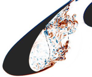
Prior to analysing the flow fluctuations, some important mean-flow characteristics from both flow topologies are presented. Streamlines and resolved TKE ( $= \frac {1}{2}(\overline {{u^\prime }^2}+\overline {{v^\prime }^2}+\overline {{w^\prime }^2})$), normalized by
  $U_\infty ^2$, are shown in figure 6. The mixing-layer path, shown as dashed red lines, is defined as the streamline passing at a point just at the outer side of the cusp. The same point is used for both configurations. The sealed case (figure 6b) also shows the return path separating the two bubbles, defined as the streamline passing at a point just at the inner side of the cusp. Using these definitions, the streamlines corresponding to the mixing-layer path and the return path were visually identified in a refined plot of streamlines in the cusp region. The highest TKE levels are observed from the reattachment region to the slat trailing edge. The maximum normalized value, whose position is marked with a white cross, is
  $0.124$ for both cases. The two-bubble case shows an additional region of high TKE upstream, with levels similar to those of the reattachment region.

Figure 6. Streamlines and resolved TKE for the (a) baseline and (b) bulb-sealed cases, respectively one- and two-bubble reference topologies. Lines indicate the (![]() ) mixing layer and the (
) mixing layer and the (![]() ) return path separating the two bubbles. The white crosses indicate the position of maximum TKE.
) return path separating the two bubbles. The white crosses indicate the position of maximum TKE.
The time-averaged spanwise vorticity ( $\overline {\omega _z}$) fields are compared in figure 7. The mixing layers display positive vorticity, but there is negative vorticity inside the cove. For the two-bubble case, this is associated with flow separation at the seal, which also prevents negative vorticity from spreading into the cove. Both scenarios show a high vorticity level at the cusp region, which attenuates and spreads as it evolves downstream. The attenuation and spreading are stronger for the two-bubble case.

Figure 7. Average spanwise vorticity for the cases of (a) one-bubble and (b) two-bubble topologies. Lines indicate the (![]() ) mixing layer and the (
) mixing layer and the (![]() ) return path between bubbles.
) return path between bubbles.
Figure 8(a) shows the central streamline of the mixing layer for both cases. It also shows segments of constant velocity-potential lines, defined as lines perpendicular to the streamlines. We generically refer to these segments as  $\eta$ and normalize their length to
  $1$. The segment locations are given as percentages of the mixing-layer path (
 $s_{ML}$) length. The TKE and spanwise vorticity profiles along these segments (
 $0 \le \eta \le 1$) are shown in figure 8(b,c), for the locations indicated in figure 8(a). Only the outer part of the mixing layer is shown because there the streamlines for both cases are similar, as observed in figure 8(a), and the analysis is more meaningful. These plots provide a more definite comparison between the two topologies. For the baseline case, the maximum TKE initially grows, reaches a saturation at approximately 60 % of the mixing-layer path and increases again towards the trailing edge. For the two-bubble case, the TKE initially increases very steeply reaching a local maximum at approximately 30 % of the mixing-layer path, after which it decays. At 80 % of this path the TKE level reaches a local minimum where the level is similar to that of the single-bubble case. From that point the TKE increases slightly more than for the single-bubble case. With regard to the TKE distribution normal to the mixing layer, the two-bubble case spreads over a wider region. However, the TKE distributions normalized by their respective maxima are similar for both cases. Regarding the vorticity distribution, figure 8(c) shows a continuous decay and spread along the mixing-layer evolution. The baseline shows higher maxima while the two-bubble case has a more even distribution, such that the integral of the vorticity in those planes is similar between the cases. In summary, we can say that the most noticeable difference is the upstream region of high TKE in the two-bubble case.

Figure 8. (a) Scheme showing segments of constant velocity-potential lines ( $\eta$) along stages of the mixing-layer path (
 $s_{ML}$). Distribution of (b) TKE and (c) time-averaged spanwise vorticity over the
  $\eta$ segments.
4. Spectral and SPOD analyses
Figure 9 shows the far-field noise spectra for one- and two-bubble topologies. These results are calculated via the Ffowcs Williams–Hawkings analogy and refer to the noise propagated from the slat near field to a position 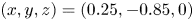 $(x, y, z) = (0.25, -0.85, 0)$ in metres or
  $(3.33, -11.33, 0)\times c_s$ relative to the slat chord. The data used for this acoustic field analysis were derived from the data used by Amaral et al. (Reference Amaral, Himeno, Souza, Pagani and Medeiros2019) which had a Strouhal number resolution (
 $St = {f c_s}/{U_\infty }$) of
  $0.088$ (
 $40$ Hz). The dotted lines also show the estimated Rossiter modes which are discussed later in the paper.
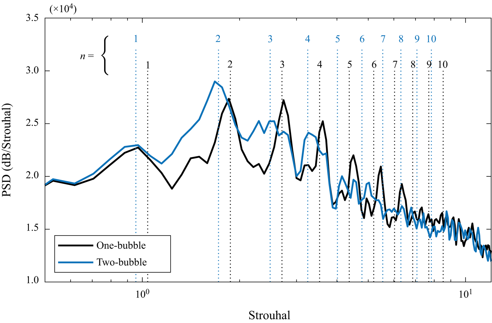

Figure 10 shows instantaneous images of the velocity fluctuations in an  $x$–
$x$– $y$ plane for both scenarios and illustrates the complexity of the flow. Consistent with the observations in figure 7, for the two-bubble case the velocity fluctuations concentrate in the primary bubble, whereas for the baseline (one-bubble case) they are more evenly spread over the slat cove. Souza et al. (Reference Souza, Rodríguez, Himeno and Medeiros2019) showed that only the two-dimensional structures contribute to the narrowband peaks of the slat noise spectra. Moreover, Amaral et al. (Reference Amaral, Himeno, Souza, Pagani and Medeiros2019) showed that at the narrowband peaks the signals in the slat cove are well correlated along the span, in particular for the two-bubble topology. For these two reasons, although the conducted lattice Boltzmann simulations are three-dimensional, the spectral and the SPOD analyses are based on the flow field at the central plane only, similarly to Souza et al. (Reference Souza, Rodríguez, Simões and Medeiros2015).

Figure 10. Typical snapshots of streamwise velocity fluctuations for (a) single-bubble and (b) two-bubble topologies.
Figure 11 shows the PSD of the streamwise velocity fluctuation as it evolves along the mixing-layer path for both cases. To produce each spectrum, the total length of the recorded time series is divided into blocks of  $1.67 \times 10^{-2}$ s. For the single-bubble case, a time series spanning
  $0.19$ s is split into 22 blocks, while for the two-bubble case we use
  $0.15$ s and 17 blocks, respectively, with 50 % overlap. The mean velocity is removed from each block. In both cases, the initial transient flow is discarded and a Hanning window is applied to each block, which is then Fourier-transformed. The resulting PSDs are averaged over the blocks. This procedure provides a Strouhal number resolution of 0.13 (
 $60$ Hz). Following Welch (Reference Welch1967), the variance
  $\sigma ^2$ in the computed PSDs using a number
  $N_b$ of blocks with 50 % overlap is given by
 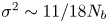 $\sigma ^2 \sim 11 / 18 N_b$. This yields
  $\sigma ^2 \approx 0.028$ for the baseline case and
  ${\sigma ^2 \approx } 0.036$ for the two-bubble case. Note that the present results may contain a non-negligible random uncertainty associated with the relatively low number of blocks. However, the predicted peaks are in good agreement with the far-field spectra (figure 9), building confidence in the validity of our results for the purposes of this work. The SPOD computations use the same sampling parameters.

Figure 11. The PSD of the streamwise velocity along the mixing-layer path for (a) single-bubble and (b) two-bubble topologies. Vertical dashed lines correspond to the Rossiter modes estimated using (4.1).
The narrowband peaks observed in the acoustic field (figure 9) reflect on the slat cove flow (Amaral et al. Reference Amaral, Himeno, Souza, Pagani and Medeiros2019). These narrowband peak Strouhal numbers are consistent with the literature (Pascioni & Cattafesta Reference Pascioni and Cattafesta2018a,Reference Pascioni and Cattafestab). The high-frequency hump is not observed in our simulations, but it is possibly very sensitive to numerical dissipation (Souza et al. Reference Souza, Rodríguez, Himeno and Medeiros2019). There is also a low-frequency noise (Strouhal number below 1 for the baseline case and below 0.5 for the two-bubble case) in the early stages of the mixing layer. It is possible that this is linked to the very-low-frequency oscillations reported by Pascioni & Cattafesta (Reference Pascioni and Cattafesta2018a,Reference Pascioni and Cattafestab) and associated with mixing-layer flapping, but our data are insufficient to investigate these oscillations.
Some narrowband peaks are better defined than others. For the baseline, the Strouhal number  $4.37$ (
 $1980$ Hz) is clearly defined, while for the two-bubble case the Strouhal number
  $1.72$ (
 $780$ Hz) is the most defined. We used these Strouhal numbers in combination with a formula proposed by Souza et al. (Reference Souza, Rodríguez, Himeno and Medeiros2019) to establish all the other Strouhal numbers in the Rossiter sequence. According to Souza et al. (Reference Souza, Rodríguez, Himeno and Medeiros2019), a mode Strouhal number is given by
 \begin{equation} St_n= \left(n+ \frac{1}{4} \right) \times \frac{c_{s}}{U_\infty} \times \frac{\overline{V_c}}{L_c + \dfrac{\overline{V_c}}{c_\infty} L_a} = \left(n+ \frac{1}{4} \right) \times St_0, \end{equation}
where  $\overline {V_c}$ is the average vortex speed along the convective path,
  $L_c$ the convective path length,
  $L_a$ the acoustic path length and
  $n$ the mode number. Equation (4.1) defines the fundamental Strouhal number (
 $St_0$) of the Rossiter sequence. In the formula, the term 1/4 accounts for a
  $90^{\circ }$ phase shift between the vortex interaction with the slat trailing edge and the sound wave emission, which was established in the analysis of Souza et al. (Reference Souza, Rodríguez, Himeno and Medeiros2019). The fundamental Strouhal number does not correspond to the first Rossiter mode Strouhal number (
 $St_1$), but to the Strouhal number shift between the modes.
Considering that the Strouhal number  $4.37$ (
 $1980$ Hz) corresponds to
  $n=5$, we obtain
  $St_0=0.83$ (
 $377$ Hz). Analogously for two-bubble topology, considering that Strouhal number
  $1.72$ (
 $780$ Hz) corresponds to
  $n=2$, we obtain
  $St_0=0.76$ (
 $347$ Hz). Based on these fundamental Strouhal numbers we can establish the Strouhal numbers of all the other modes, which we refer to as
  $R_n$ (
 $n = 1, 2, 3,\ldots$), summarized in table 2.
Table 2. Estimated Rossiter mode Strouhal numbers and frequencies based on (4.1) proposed by Souza et al. (Reference Souza, Rodríguez, Himeno and Medeiros2019).

The calculated Strouhal numbers are marked in figures 11 and 9 as dashed lines. There is good agreement where the peaks are better defined in the acoustic far field and along the mixing layer. Except for the very-low-frequency noise ( $St<0.1$), the baseline is remarkably quiet close to the cusp. Downstream, the narrowband peaks emerge, starting with the higher-frequency peaks and evolving to lower frequencies as the trailing edge is approached. For the two-bubble case there is about two orders of magnitude higher activity close to the cusp throughout the frequency range considered. In this region, the spectral peaks are poorly defined as if immersed in noise. Further downstream, low-frequency narrowband peaks emerge from the noise in a pattern that resembles the baseline case, but is less clear. In comparison with the baseline, the two-bubble case is dominated by lower Rossiter modes.
The spectral plots permit the selection of the relevant frequencies for the SPOD analysis described in § 2.2. The SPOD technique is applied to all frequencies indicated in the spectra in figure 11. For both cases, the first SPOD mode accounts for over 99 % of the pressure–intensity correlation used (see figure 12). We note that, because of the frequency discretization of  $60$ Hz (
 ${\rm \Delta} St=0.13$), for the SPOD analysis we use the closest possible frequency. Figure 13 displays contour plots of the real part of the first SPOD mode for all of the selected frequencies, for the one- and two-bubble cases. The figure suggests K–H structures evolving along the mixing layer. Consistently, the lower frequencies display higher wavelengths.

Figure 12. The POD eigenvalues for (a) single-bubble and (b) two-bubble topologies.

Figure 13. Real part of the first SPOD mode for (a) one-bubble (baseline) and (b) two-bubble cases at selected frequencies. Dashed lines indicate the mixing layers of both cases and the return path of the two-bubble case.
The amplitude distribution of the complex SPOD modes is displayed in figure 14. The plots are normalized by the maximum value, whose location in each frame is indicated by a cross symbol. Hence, these plots cannot be used to compare the relative magnitude of the modes, for which the spectral plots (figure 11) should be used. In comparison with the spectral analysis (figure 11), the SPOD analysis shows more clearly that the lower Rossiter modes are more active further from the cusp.

Figure 14. Magnitude of the first SPOD mode for (a) one-bubble and (b) two-bubble cases. Dashed lines indicate the mixing layers of both cases and the return path of the two-bubble case.
The spectral analysis also shows that the fundamental Strouhal number of the Rossiter modes ( $St_0$) in the two-bubble case is lower than that of the baseline. Regarding (4.1), Souza et al. (Reference Souza, Rodríguez, Himeno and Medeiros2019) defined
  $St_0 = (c_{s}/U_\infty )(T_c+T_a)^{-1}$, where
  $T_c = L_c/\overline {V_c}$ and
  $T_a = L_a/c_\infty$ (
 $c_\infty$ is the speed of sound) correspond to the convective and acoustic times, respectively. It is important to investigate whether these times are consistent with the Rossiter feedback model for the topologies studied. Souza et al. (Reference Souza, Rodríguez, Himeno and Medeiros2019) defined the convective path as the path taken by the dominant SPOD structures. They also point out that this path is essentially the dividing streamline of the mixing layer, except very close to the reattachment point, where it deviates towards the slat trailing edge.
Figure 15 shows the acoustic and convective paths considered in the current analysis. The acoustic path is defined as the straight line connecting the slat trailing edge and the cusp. For both cases, the acoustic path lengths are identical,  $L_a = 0.82 \times c_s$ (
 $61.4$ mm), which leads to the non-dimensional acoustic time
  $T_a \times U_\infty /c_s=0.082$. For the baseline and the two-bubble case, we choose respectively modes
  $R_5$ and
  $R_2$ as reference of the convective path, based on a compromise between relevance of the mode and clarity of the path. While this is somewhat arbitrary, the results are not very sensitive to this choice. The lengths of the convective paths are
 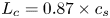 $L_c = 0.87 \times c_s$ (
 $65.2$ mm) and
  $L_c = 0.86 \times c_s$ (
 $64.8$ mm) for the one- and two-bubble cases, respectively. For each case, we calculate the velocity component (
 $V_c$) tangent to the convective path, shown in figure 16. The convective time (
 $T_c$) is calculated by integrating the inverse of
  $V_c$ along its path. Even though the mixing layers dividing streamlines are almost identical (see figure 8), the velocity magnitude differs and the convective time increases from
  $T_c \times U_\infty /c_s = 1.1$ for the one-bubble case to
  $1.2$ for the two-bubble case. Finally, with
  $T_a$ and
  $T_c$ values, we find
  $St_0 = 0.85$ (
 $385$ Hz) and
  $St_0 = 0.78$ (
 $352$ Hz) for the one- and two-bubble cases, respectively. These estimates are within an accuracy of 3 % relative to the values used to produce table 2.

Figure 15. Magnitude of modes  $R_5$ and
  $R_2$ from cases of (a) one-bubble and (b) two-bubble topologies (see figure 14) indicating the (
![]() ) convective paths of the structures and their respective (
) convective paths of the structures and their respective (![]() ) acoustic paths. For reference, the mixing layers and return path are also shown as yellow continuous and dotted lines, respectively.
) acoustic paths. For reference, the mixing layers and return path are also shown as yellow continuous and dotted lines, respectively.

Figure 16. Convective velocity ( $V_c$) along the convective paths indicated in figure 15.
5. Spanwise vorticity structures
This section aims at identifying in the flow evolution the structures elicited by the SPOD analysis. It also aims at understanding their origin. For this purpose we investigate supplementary movie 1 available at https://doi.org/10.1017/jfm.2021.93, as well as sequences of snapshots of the spanwise vorticity in the central  $x$–
$x$– $y$ plane of the simulation (figure 17).

Figure 17. Instantaneous spanwise vorticity inside the slat cove along 10 frames spaced by  $1.42 \times 10^{-4}\ {\rm s}$ which covers a time period corresponding to Strouhal number
  $1.72$ (
 $782$ Hz) for (a) one-bubble and (b) two-bubble cases. Dashed lines indicate the mixing layers of both cases and the return path of the two-bubble case.
In the baseline case flow, the mixing layer is rather quiet and steady close to the cusp. Fine-grained turbulence is present in the slat cove which recirculates slowly and interacts mildly with the mixing layer in this region. Vortices of small wavelength become observable downstream, between 20 % and 40 % of the mixing-layer path. These vortices evolve into wider and more complex vortical structures further downstream. The two-bubble case presents a much stronger interaction between the recirculating vorticity and the mixing layer: vortices are formed at an earlier stage in comparison with the baseline case, nearly immediately at the cusp. Further downstream, the vortices evolve into wider and more complex vortical structures.
The frequency-domain structures educed by the SPOD are not readily identifiable in supplementary movie 1 or in figure 17. To facilitate their identification in time and space evolution along the mixing layer, the grid formed by the streamlines and equipotential lines of the slat cove mixing layer is mapped onto an equivalent Cartesian grid, as shown in figure 18. Only the outer part of the mixing layer is used. For the two-bubble case, the internal streamlines involve the return path and it would be difficult to interpret their role in the transformed grid. On the other hand, the external streamlines are very similar for both cases, facilitating comparison. Figure 19 shows a number of snapshots of the spanwise vorticity fields in the transformed grid. For both cases, the frames cover the time interval  $3.84 \times 10^{-3}$. The spatio-temporal evolution of the vortical structures, showing the formation of vortices and their downstream evolution, allows the identification of wavelengths and frequencies that can be used to relate the vortex dynamics to the results of the spectral/SPOD analysis.

Figure 18. Instantaneous spanwise vorticity of frame 10 from the one-bubble case (figure 17) and mesh composed of the intersection points between the streamlines and equipotential lines,  $\varPsi _i$ and
  $\varPhi _j$, shown both in their original coordinates and also in orthogonal axes.

Figure 19. Instantaneous spanwise vorticity for (a) one-bubble and (b) two-bubble slat cove flow cases along a time interval of  $3.84 \times 10^{-3}$ s, which corresponds to a Strouhal number of
  $0.57$ (
 $260.6$ Hz). The contours are plotted along a mesh composed of transformed streamlines and equipotential lines (see figure 8a). Results shown in figure 17 correspond to frames 10 to 19 of this figure. The colourbar is the same as that of figures 17 and 18.
Figure 19(a) shows the vorticity evolution for the baseline case. The formation of K–H vortices occurs in an apparently irregular fashion. These vortices widen as they travel along the mixing layer, in a manner consistent with the frequency-domain analyses that show a progressive cascade towards lower Rossiter modes (figure 11). The time interval shown in the figure corresponds to slightly more than six periods of the mode  $R_4$. In the time evolution at the fixed location of approximately
  $70\,\%$ of the mixing-layer path, six or more vortex structures can be observed, even if not in a completely periodic sequence. Thus, the observed evolution is consistent with the spectral analysis that shows the predominance of the modes
  $R_4$ and higher in this region.
Figure 19(b) shows the vorticity evolution for the two-bubbles case. The vortex structures are more complex and wider than in the baseline case. However, in the time evolution at the fixed location, their temporal periodicity is more regular than for the baseline, in particular at the trailing edge. There we see three time periods of a broader structure arriving at the trailing-edge region in the time interval shown, which incidentally corresponds to approximately three periods of the mode  $R_2$ for this case. These structures have a spatial periodicity of about half of the mixing-layer path, which further relates them to the mode
  $R_2$ recovered by the SPOD. The spectral analysis (figure 11) suggests that mode
  $R_2$ is dominant over a large portion of the mixing-layer path and that higher Rossiter modes are observable only in the initial stages of evolution, e.g. the compact vortex structures seen up to approximately
  $20\,\%$ of the mixing layer.
Comparing the results from the baseline and the two-bubble case, it is found that later structures of the baseline resemble structures of an earlier stage in the two-bubble case. For example, the structures at 80 % of the mixing layer in frames 0 to 3 for the baseline case resemble those at 30 % of the mixing layer in frames 10 to 13 for the two-bubble case (see region indicated by black continuous lines in figure 19). As a second example, the structure at  $70\,\%$ of the mixing layer in frame 25 for the baseline case resembles that at
  $40\,\%$ of the mixing layer in frame 17 for the two-bubble case (see region indicated by black dashed lines in figure 19). This suggests that the two-bubble case develops more quickly or bypasses some stages of the evolution. This aspect is associated with the origin of these structures that we address next.
With the aid of figure 19 we can more easily interpret figure 17 and supplementary movie 1. Note that the frames in figure 17 correspond to frames 10 to 19 in the red box in figure 19. Supplementary movie 1 shows results for the baseline and the two-bubble case which are synchronized to facilitate comparison. They correspond to four times the time interval shown in figure 18, e.g. 12 periods of mode  $R_2$ of the two-bubble case. As discussed above, the baseline case presents compact vortices which gradually develop into wider and more complex structures. The latter structures are associated with the intermediate Rossiter modes (
 $R_4$ and
  $R_6$), which are evinced closer to the reattachment point in the SPOD analysis. The spatio-temporal evolution of these vortical structures resemble those discussed by Trieling, Fuentes & van Heijst (Reference Trieling, Fuentes and van Heijst2005), who investigated the interaction of two unequal co-rotating vortices. They refer to the phenomena observed as vortex straining and vortex merging; both phenomena coexist, but their relative importance depends on the relative magnitude and distance of the vortices. A dominant feature is the formation of a wide vortical structure composed of vorticity filaments surrounding a vortex core, as observed in supplementary movie 1 and in figure 19. In the slat cove flow, considerably more complex than that studied by Trieling et al. (Reference Trieling, Fuentes and van Heijst2005), the incoherent turbulence recirculating in the cove presents both positive and negative vorticity. This turbulence is engulfed in the process and contributes to the formation of vortex clusters, which dominate the flow dynamics beyond
  $60\,\%$ of the mixing-layer path. These clusters continue entrapping the recirculating vorticity and widening and, as seen in supplementary movie 1, occasionally experience a process akin to vortex pairing in the reattachment region. This gives rise to the clusters associated with modes
  $R_2$ and
  $R_3$ that both the spectral and SPOD analyses identify only very close to the reattachment region. Sometimes the small-wavelength vortices at the early stages of the mixing layer also exhibit vortex pairing, but, as shown in supplementary movie 1, it seems a less common event in this flow. It is interesting to note in passing that while the SPOD suggests classical K–H vortices, the typical structures are much more complex than that. They are very distorted, but, on average, with a remarkably regular core captured by the SPOD analysis.
For the two-bubble case, supplementary movie 1 and figure 17 indicate an intense recirculation of vorticity within the primary bubble, following the return path. Relative to the baseline recirculation path, the return path is shorter and the speed along it is higher. These differences enhance both the recirculation and the interaction of the recirculating vorticity with the mixing layer. The return path streamline indicates that the recirculating vorticity can be convected to regions very close to the slat cusp. At locations below 20 % of the mixing-layer path, supplementary movie 1 and figure 17 show that the recirculating vorticity is entrapped by the K–H vortices, forming structures that resemble the later structures of the baseline. A very strong interaction between the primary clusters and recirculating vorticity occurs at approximately  $40\,\%$ of the mixing-layer path. First, the primary clusters in the mixing layer are already developed in this region and can entrap recirculating vorticity from further away from the mixing layer, in comparison with the initial compact vortices. Second, because of the higher speed in the return path, the recirculating vorticity seems to impinge onto these primary clusters. The strong interactions destroy the coherence of the higher Rossiter modes (say above
  $R_5$; see figure 14), while promoting the formation of very wide clusters. These mature clusters are very distorted structures, with both positive and negative vorticity, but in general still exhibit a slow counterclockwise rotation, more easily observed in supplementary movie 1. For the reasons discussed before, these dominant vortical structures are associated with Rossiter mode
  $R_2$. Figure 14(b) suggests that the formation of the mode
  $R_2$ is augmented by the recirculation of structures with the same frequency (see the circular arrow in the
  $R_2$ frame of figure 14b). The location where this mode becomes observable is also very regular and constitutes a local maximum in the SPOD magnitude distribution. Its immediate decay may be a manifestation of the complexity of the resulting structure as it is convected. In the reattachment region a second amplitude maximum is reached as occurs for most other modes, specially
  $R_3$ and
  $R_4$. In supplementary movie 1, mode
  $R_2$ can be more easily identified by observing its periodicity close to the trailing edge.
It is interesting that the strong interaction with the recirculating vorticity does not disrupt the Rossiter frequency selection mechanism, except by changing the dominant mode. The recirculation of structures oscillating with the same frequency of mode  $R_2$ for the two-bubble case certainly contributes to the robustness of this mode. Moreover, mode
  $R_2$ may help to stabilize the frequency of all other modes. The results also suggest that most interactions constitute engulfment of random and weak vorticity by vortices or vorticity clusters. In both cases, the engulfed vorticity does not substantially displace the structure core.
6. Conclusions
An important part of slat noise is composed of narrowband spectral peaks, which are known to be associated with a Rossiter acoustic feedback mechanism. It has been demonstrated (Amaral et al. Reference Amaral, Himeno, Souza, Pagani and Medeiros2019) that a bulb seal can produce a counter-rotating secondary recirculating bubble and enhance noise emission. In this work, the flow fluctuations inside a slat cove with and without a bulb seal are compared. The seal position is chosen to produce the secondary bubble while the single-bubble scenario corresponds to the baseline configuration, with no seal. The recirculation of turbulence in the primary bubble of the two-bubble case is much stronger than for the baseline. This produces a region of large TKE close to the slat cusp, which does not appear in the baseline configuration.
A spectral analysis demonstrates that, in both cases, the narrowband peak frequencies conform with the formula proposed by Souza et al. (Reference Souza, Rodríguez, Himeno and Medeiros2019), which includes a  ${\rm \pi} /2$ phase shift between the interaction of the vortices with the slat trailing edge and the emission of the sound wave. A SPOD analysis was conducted for the peak frequencies, which considers an ad hoc correlation matrix involving only the acoustic pressure radiated from the slat cove region. Our results show a cascade of progressively lower Rossiter modes along the mixing-layer evolution for both cases. For the single-bubble case, the cascade initiates earlier and progresses much more rapidly leading to the predominance of lower Rossiter modes. Calculations of the convective time of the SPOD structure and the acoustic time provided very accurate predictions of the Rossiter mechanism fundamental frequency.
Guided by the SPOD analysis, we identified the actual Rossiter mode structures in spanwise vorticity fields. For the baseline, the initially dominant high-frequency Rossiter modes (above mode  $R_6$) are regular K–H vortices, while the latterly dominant, intermediate Rossiter modes (modes
  $R_4$ to
  $R_6$) are clusters of vorticity composed of a core and filaments of vorticity surrounding the core. The spectrum composed of narrowband peaks manifests itself in physical space as structures modulated in amplitude and wavelength. The interaction of vortices of different magnitude gives rise to phenomena like vortex straining and merging (Trieling et al. Reference Trieling, Fuentes and van Heijst2005), leading to the vortex clusters observed in the slat cove. For the two-bubble case, such clusters are observed at a much earlier stage. The latterly dominant, low-frequency Rossiter modes (mostly
  $R_2$) are much more complex and wider structures composed of positive and negative vorticity, slowly rotating according to the mixing layer. A substantial part of these wide structures is composed of recirculating vorticity which was engulfed into the clusters. Even though the structures are complex and every realization differs from another in detail, the core behaves very regularly as demonstrated by the SPOD analysis.
The origin of these large structures is tracked down to a very strong interaction between the mixing layer and the vorticity recirculating in the primary bubble of the two-bubble case. This stronger interaction is promoted by the fact that, in this scenario, the recirculation path is substantially shorter and the speed along the path substantially higher. Of particular importance is that along this path there is recirculation of structures that oscillate at the same frequency as mode  $R_2$. On average, this interaction happens at a well-defined place, approximately 40 % of the mixing-layer path for this particular configuration. At this position, the coherence of higher Rossiter modes is severely destroyed and mode
  $R_2$ is greatly enhanced. This location also corresponds to the region of large TKE close to the slat cusp in the two-bubble case. Overall, these results indicate that a significant part of this TKE is not associated with random turbulence but with coherent structures.
The seal also distorts the slat cove mean flow by reducing the convective velocity of the structures and hence the fundamental frequency of the Rossiter mechanism. This is, however, a minor effect. It is interesting that although in the two-bubble case the interaction with recirculating vorticity is very strong, it does not disrupt the Rossiter frequency selection mechanism. This is thought to be a consequence of the fact that part of the recirculating vorticity remains coherent. Also, the nature of the interaction, consisting mostly of vorticity engulfment, does not involve significant displacement of the cluster core. The interaction only greatly accelerates the process towards lower Rossiter modes.
Supplementary movie
Supplementary movie is available at https://doi.org/10.1017/jfm.2021.93.
Acknowledgements
The authors are grateful to EMBRAER, EXA Corp and Núcleo de Dinâmica dos Fluidos (NDF/USP) for providing the PowerFLOW licence.
Funding
F.H.T.H. received financial support from São Paulo Research Foundation (FAPESP/Brazil; grant nos. 2016/02970-5 and 2018/02542-9). D.S.S. and F.R.A. received funding from Coordination for the Improvement of Higher Education Personnel (CAPES/Brazil; grant no. DS00011/07-0). F.R.A. also received funding from FAPESP/Brazil (grant no. 2019/02203-2). D.R. acknowledges funding by the National Council for Scientific and Technological Development (CNPq/Brazil; grant nos. 405144/2016-4 and 305512/2016-1) and from Rio de Janeiro Research Foundation FAPERJ/Brazil (grants E-26/010.000356/2017 and E-26/200.003/2018). D.R. also acknowledges funding by the Government of the Community of Madrid within the multi-annual agreement with Universidad Politécnica de Madrid (V PRICIT, line 3) through the Program of Excellence in Faculty and the Program of Impulse of Young Researchers (grant no. APOYO-JOVENES-WYOWRI-135-DZBLJU). M.A.F.M. is sponsored by CNPq/Brazil (grant no. 307956/2019-9). The initial stages of this research were financed by FAPESP/Brazil (grant no. 2006/52568-7). D.S.S and M.A.F.M acknowledge support from Marie Curie Grant PIRSES-GA-2009-247651 (FP7-PEOPLE-IRSES: ICOMASEF, Instability and COntrol of MAssively SEparated Flows).
Declaration of interests
The authors report no conflict of interest.


