


1 Introduction
The transport of heat and mass (i.e. scalar) in wall-bounded turbulent flows has attracted significant attention in the past several decades. In particular, similarity arguments developed for the velocity field have been successfully extended to the scalar field when the molecular Prandtl number Pr is close to unity (see, for example, Monin & Yaglom Reference Monin and Yaglom1971; Townsend Reference Townsend1976; Kader Reference Kader1981; Subramanian & Antonia Reference Subramanian and Antonia1981; Nagano & Tagawa Reference Nagano and Tagawa1988). Also, an increased use has been made of direct numerical simulations (DNSs) to understand the underlying physics of turbulence since these provide detailed spatial and temporal information with high accuracy. The seminal work by Kim & Moin (Reference Kim, Moin, André, Cousteix, Durst, Launder, Schmidt and Whitelaw1989) dealt with a passive scalar transport in a turbulent channel flow with a Kármán number
 $h^{+}(\equiv U_{\unicode[STIX]{x1D70F}}h/\unicode[STIX]{x1D708})=180$
and three values (0.2, 0.71 and 2.0) of the molecular Prandtl number Pr. Here,
$h^{+}(\equiv U_{\unicode[STIX]{x1D70F}}h/\unicode[STIX]{x1D708})=180$
and three values (0.2, 0.71 and 2.0) of the molecular Prandtl number Pr. Here,
 $h^{+}$
represents the ratio of the half-width of the channel
$h^{+}$
represents the ratio of the half-width of the channel
 $h$
and the viscous length scale
$h$
and the viscous length scale
 $\unicode[STIX]{x1D708}/U_{\unicode[STIX]{x1D70F}}$
(
$\unicode[STIX]{x1D708}/U_{\unicode[STIX]{x1D70F}}$
(
 $U_{\unicode[STIX]{x1D70F}}(\equiv (\unicode[STIX]{x1D70F}_{w}/\unicode[STIX]{x1D70C})^{1/2})$
is the friction velocity, where
$U_{\unicode[STIX]{x1D70F}}(\equiv (\unicode[STIX]{x1D70F}_{w}/\unicode[STIX]{x1D70C})^{1/2})$
is the friction velocity, where
 $\unicode[STIX]{x1D70F}_{w}$
is the wall shear stress and
$\unicode[STIX]{x1D70F}_{w}$
is the wall shear stress and
 $\unicode[STIX]{x1D70C}$
is the density of the fluid; the superscript
$\unicode[STIX]{x1D70C}$
is the density of the fluid; the superscript
 $+$
denotes normalization by wall units). They used an internal heating source so that the passive scalar was created internally and removed from two isothermal walls. Since then, several DNS studies have been performed in a turbulent channel flow with passive scalar transport for higher Reynolds numbers and various thermal boundary conditions (Johansson & Wikström Reference Johansson and Wikström1999; Kawamura, Abe & Matsuo Reference Kawamura, Abe and Matsuo1999; Morinishi, Tamano & Nakamura Reference Morinishi, Tamano and Nakamura2003; Abe, Kawamura & Matsuo Reference Abe, Kawamura and Matsuo2004a
; Abe, Antonia & Kawamura Reference Abe, Antonia and Kawamura2009; Antonia, Abe & Kawamura Reference Antonia, Abe and Kawamura2009; Hasegawa & Kasagi Reference Hasegawa and Kasagi2011; Saruwatari & Yamamoto Reference Saruwatari and Yamamoto2014; Pirozzoli, Bernardini & Orlandi Reference Pirozzoli, Bernardini and Orlandi2016). In these studies, the functional Re and Pr dependence of mean and turbulence quantities relating to the scalar dissipation function (defined in (1.19)) has been examined intensively. As for the velocity field (Kaneda, Morishita & Ishihara Reference Kaneda, Morishita and Ishihara2013; Lee & Moser Reference Lee and Moser2015), the maximum
$+$
denotes normalization by wall units). They used an internal heating source so that the passive scalar was created internally and removed from two isothermal walls. Since then, several DNS studies have been performed in a turbulent channel flow with passive scalar transport for higher Reynolds numbers and various thermal boundary conditions (Johansson & Wikström Reference Johansson and Wikström1999; Kawamura, Abe & Matsuo Reference Kawamura, Abe and Matsuo1999; Morinishi, Tamano & Nakamura Reference Morinishi, Tamano and Nakamura2003; Abe, Kawamura & Matsuo Reference Abe, Kawamura and Matsuo2004a
; Abe, Antonia & Kawamura Reference Abe, Antonia and Kawamura2009; Antonia, Abe & Kawamura Reference Antonia, Abe and Kawamura2009; Hasegawa & Kasagi Reference Hasegawa and Kasagi2011; Saruwatari & Yamamoto Reference Saruwatari and Yamamoto2014; Pirozzoli, Bernardini & Orlandi Reference Pirozzoli, Bernardini and Orlandi2016). In these studies, the functional Re and Pr dependence of mean and turbulence quantities relating to the scalar dissipation function (defined in (1.19)) has been examined intensively. As for the velocity field (Kaneda, Morishita & Ishihara Reference Kaneda, Morishita and Ishihara2013; Lee & Moser Reference Lee and Moser2015), the maximum
 $h^{+}$
in the DNS has increased significantly for the scalar field and is now around 4000 (Pirozzoli et al.
Reference Pirozzoli, Bernardini and Orlandi2016). It became recently evident that the mean scalar obeys the generalized logarithmic law in the lower half of the channel and a parabolic defect profile in the core region (see Pirozzoli et al.
Reference Pirozzoli, Bernardini and Orlandi2016).
$h^{+}$
in the DNS has increased significantly for the scalar field and is now around 4000 (Pirozzoli et al.
Reference Pirozzoli, Bernardini and Orlandi2016). It became recently evident that the mean scalar obeys the generalized logarithmic law in the lower half of the channel and a parabolic defect profile in the core region (see Pirozzoli et al.
Reference Pirozzoli, Bernardini and Orlandi2016).
One of the important quantities to be obtained accurately is the heat transfer coefficient (or equivalently the Stanton number), viz.
 $$\begin{eqnarray}h_{t}\equiv Q_{w}/\unicode[STIX]{x1D70C}C_{p}U_{b}T_{m}=1/U_{b}^{+}T_{m}^{+},\end{eqnarray}$$
where
 $Q_{w}=\unicode[STIX]{x1D70C}C_{p}U_{\unicode[STIX]{x1D70F}}T_{\unicode[STIX]{x1D70F}}$
and
$Q_{w}=\unicode[STIX]{x1D70C}C_{p}U_{\unicode[STIX]{x1D70F}}T_{\unicode[STIX]{x1D70F}}$
and
 $C_{p}$
are the wall heat flux and specific heat at the constant pressure, respectively;
$C_{p}$
are the wall heat flux and specific heat at the constant pressure, respectively;
 $T_{\unicode[STIX]{x1D70F}}$
is the friction temperature. Here,
$T_{\unicode[STIX]{x1D70F}}$
is the friction temperature. Here,
 $U_{b}$
and
$U_{b}$
and
 $T_{m}$
are the bulk mean velocity and the mixed mean (or sometimes bulk mean) temperature, respectively, defined such that
$T_{m}$
are the bulk mean velocity and the mixed mean (or sometimes bulk mean) temperature, respectively, defined such that
 $$\begin{eqnarray}U_{b}\equiv \frac{1}{h}\int _{0}^{h}\bar{U}\,\text{d}y\end{eqnarray}$$
and
 $$\begin{eqnarray}T_{m}\equiv \frac{1}{h}\int _{0}^{h}\frac{\bar{U}\bar{\unicode[STIX]{x1D6E9}}}{U_{b}}\,\text{d}y.\end{eqnarray}$$
The form of
 $h_{t}$
is analogous to that of the skin friction coefficient, viz.
$h_{t}$
is analogous to that of the skin friction coefficient, viz.
 $$\begin{eqnarray}C_{f}\equiv \unicode[STIX]{x1D70F}_{w}/{\textstyle \frac{1}{2}}\unicode[STIX]{x1D70C}U_{b}^{2}=2/U_{b}^{+\,2}.\end{eqnarray}$$
The perfect analogy between
 $C_{f}$
and
$C_{f}$
and
 $h_{t}$
(i.e.
$h_{t}$
(i.e.
 $C_{f}=2h_{t}$
) is referred to as the Reynolds analogy.
$C_{f}=2h_{t}$
) is referred to as the Reynolds analogy.
Significant attention was given to the possible
 $h^{+}$
dependence of
$h^{+}$
dependence of
 $C_{f}$
on the basis of the mean velocity log law. Recently, Zanoun, Nagib & Durst (Reference Zanoun, Nagib and Durst2009) observed that the logarithmic skin friction relation
$C_{f}$
on the basis of the mean velocity log law. Recently, Zanoun, Nagib & Durst (Reference Zanoun, Nagib and Durst2009) observed that the logarithmic skin friction relation
 $$\begin{eqnarray}U_{b}^{+}=\frac{1}{\unicode[STIX]{x1D705}}\ln (h^{+})-\frac{1}{\unicode[STIX]{x1D705}}+A\end{eqnarray}$$
or, equivalently,
 $$\begin{eqnarray}\sqrt{\frac{2}{C_{f}}}=\frac{1}{\unicode[STIX]{x1D705}}\ln (Re_{b}\sqrt{C_{f}}/2\sqrt{2})-\frac{1}{\unicode[STIX]{x1D705}}+A\end{eqnarray}$$
obtained from the logarithmic law of the wall
 $$\begin{eqnarray}U^{+}=\frac{1}{\unicode[STIX]{x1D705}}\ln (y^{+})+A\end{eqnarray}$$
(
 $\unicode[STIX]{x1D705}$
and
$\unicode[STIX]{x1D705}$
and
 $A$
denote the von Kármán constant and the additive constant, respectively), with
$A$
denote the von Kármán constant and the additive constant, respectively), with
 $\unicode[STIX]{x1D705}=0.37$
and
$\unicode[STIX]{x1D705}=0.37$
and
 $A=3.7$
, as obtained by Zanoun, Durst & Nagib (Reference Zanoun, Durst and Nagib2003) represents more accurately the experimental skin friction data than Dean’s (Reference Dean1978) formula,
$A=3.7$
, as obtained by Zanoun, Durst & Nagib (Reference Zanoun, Durst and Nagib2003) represents more accurately the experimental skin friction data than Dean’s (Reference Dean1978) formula,
 $$\begin{eqnarray}C_{f}=0.073Re_{b}^{-1/4},\end{eqnarray}$$
in particular, for
 $h^{+}>2000$
(see figure 5 of their paper).
$h^{+}>2000$
(see figure 5 of their paper).
Likewise, a possible
 $h^{+}$
dependence of
$h^{+}$
dependence of
 $h_{t}$
was examined on the basis of scalar log law. Monin & Yaglom (Reference Monin and Yaglom1971) (see also Kader & Yaglom (Reference Kader and Yaglom1972)) assumed that the logarithmic defect laws for both velocity and scalar are valid up to channel/pipe centreline and obtained a relation for the mixed mean scalar with respect to the Reynolds number, i.e.
$h_{t}$
was examined on the basis of scalar log law. Monin & Yaglom (Reference Monin and Yaglom1971) (see also Kader & Yaglom (Reference Kader and Yaglom1972)) assumed that the logarithmic defect laws for both velocity and scalar are valid up to channel/pipe centreline and obtained a relation for the mixed mean scalar with respect to the Reynolds number, i.e.
 $$\begin{eqnarray}T_{m}=\unicode[STIX]{x1D6FC}\ln (Re_{b}\sqrt{C_{f}})+\unicode[STIX]{x1D6FE}(Pr),\end{eqnarray}$$
where
 $\unicode[STIX]{x1D6FC}$
and
$\unicode[STIX]{x1D6FC}$
and
 $\unicode[STIX]{x1D6FE}$
are constants and
$\unicode[STIX]{x1D6FE}$
are constants and
 $Re_{b}$
denotes the Reynolds number based on
$Re_{b}$
denotes the Reynolds number based on
 $U_{b}$
and the channel/pipe width. Kader & Yaglom (Reference Kader and Yaglom1972) examined the experimental data in a channel, pipe and boundary layer and noted that
$U_{b}$
and the channel/pipe width. Kader & Yaglom (Reference Kader and Yaglom1972) examined the experimental data in a channel, pipe and boundary layer and noted that
 $\unicode[STIX]{x1D6FC}(=2.12)$
is independent of Pr and the product of the turbulent Prandtl number
$\unicode[STIX]{x1D6FC}(=2.12)$
is independent of Pr and the product of the turbulent Prandtl number
 $Pr_{t}(=0.85)$
and
$Pr_{t}(=0.85)$
and
 $1/\unicode[STIX]{x1D705}(=0.4)$
while
$1/\unicode[STIX]{x1D705}(=0.4)$
while
 $\unicode[STIX]{x1D6FE}$
depends on Pr. They also tested the resulting heat transfer coefficient
$\unicode[STIX]{x1D6FE}$
depends on Pr. They also tested the resulting heat transfer coefficient
 $h_{t}$
, i.e.
$h_{t}$
, i.e.
 $$\begin{eqnarray}h_{t}=\frac{\sqrt{(C_{f}/2)}}{\unicode[STIX]{x1D6FC}\ln (Re_{b}\sqrt{C_{f}})+\unicode[STIX]{x1D6FE}(Pr)},\end{eqnarray}$$
in a pipe flow for
 $Pr=0.71$
against large amount of experimental data. They stated that the agreement with the experimental data is excellent except for
$Pr=0.71$
against large amount of experimental data. They stated that the agreement with the experimental data is excellent except for
 $Re_{b}<2\times 10^{4}$
(
$Re_{b}<2\times 10^{4}$
(
 $R^{+}<500$
–600) where the well-known power-law relation of Kays (Reference Kays1966) given by
$R^{+}<500$
–600) where the well-known power-law relation of Kays (Reference Kays1966) given by
 $$\begin{eqnarray}h_{t}=0.018Re_{b}^{-0.2}Pr^{-0.5}\end{eqnarray}$$
fits the data slightly better than (1.10) (see also figure 2 of their paper).
On the other hand, a different approach can be taken for establishing possible
 $h^{+}$
dependences for both
$h^{+}$
dependences for both
 $C_{f}$
and
$C_{f}$
and
 $h_{t}$
with the use of energy balances for both mean and turbulent parts (i.e. via a global energy balance). In this context, Abe & Antonia (Reference Abe and Antonia2016) examined the relationship between the skin friction coefficient
$h_{t}$
with the use of energy balances for both mean and turbulent parts (i.e. via a global energy balance). In this context, Abe & Antonia (Reference Abe and Antonia2016) examined the relationship between the skin friction coefficient
 $C_{f}$
and the energy dissipation function
$C_{f}$
and the energy dissipation function
 $E$
(Rotta Reference Rotta1962), consisting of mean and turbulent parts, i.e.
$E$
(Rotta Reference Rotta1962), consisting of mean and turbulent parts, i.e.
 $$\begin{eqnarray}E\equiv \underbrace{\unicode[STIX]{x1D708}\overline{u_{i,j}(u_{i,j}+u_{j,i})}}_{\overline{\unicode[STIX]{x1D700}}}+\underbrace{\unicode[STIX]{x1D708}\overline{U}_{i,j}(\overline{U}_{i,j}+\overline{U}_{j,i})}_{\overline{\unicode[STIX]{x1D700}}_{mean}},\end{eqnarray}$$
using their DNS database in a turbulent channel flow together with other DNS and experimental data up to
 $h^{+}=10^{4}$
. Note that
$h^{+}=10^{4}$
. Note that
 $u_{1}$
,
$u_{1}$
,
 $u_{2}$
,
$u_{2}$
,
 $u_{3}$
denote the streamwise, wall-normal and spanwise velocity fluctuations, respectively;
$u_{3}$
denote the streamwise, wall-normal and spanwise velocity fluctuations, respectively;
 $u$
,
$u$
,
 $v$
,
$v$
,
 $w$
are used interchangeably with
$w$
are used interchangeably with
 $u_{1}$
,
$u_{1}$
,
 $u_{2}$
,
$u_{2}$
,
 $u_{3}$
;
$u_{3}$
;
 $\unicode[STIX]{x1D708}$
denotes the kinematic viscosity and the overbar denotes averaging with respect to
$\unicode[STIX]{x1D708}$
denotes the kinematic viscosity and the overbar denotes averaging with respect to
 $x$
,
$x$
,
 $z$
(
$z$
(
 $x$
,
$x$
,
 $y$
,
$y$
,
 $z$
are the streamwise, wall-normal and spanwise directions, respectively) and
$z$
are the streamwise, wall-normal and spanwise directions, respectively) and
 $t$
(time); upper cases denote instantaneous quantities. Given that the total energy dissipated in the channel is equal to the energy input via the mean pressure gradient, the energy balance was given by
$t$
(time); upper cases denote instantaneous quantities. Given that the total energy dissipated in the channel is equal to the energy input via the mean pressure gradient, the energy balance was given by
 $$\begin{eqnarray}E=-\frac{1}{\unicode[STIX]{x1D70C}}\frac{\text{d}\bar{P}}{\text{d}x}U_{b}h=U_{\unicode[STIX]{x1D70F}}^{2}U_{b}\quad \text{or equivalently},\quad U_{b}^{+}=E/U_{\unicode[STIX]{x1D70F}}^{3}.\end{eqnarray}$$
It was noted that the logarithmic skin friction law, established on the basis of (1.13), viz.
 $$\begin{eqnarray}U_{b}^{+}(\equiv U_{b}/U_{\unicode[STIX]{x1D70F}})=2.54\ln (h^{+})+2.41,\end{eqnarray}$$
or, equivalently,
 $$\begin{eqnarray}\frac{1}{\sqrt{C_{f}}}=1.80\ln (Re_{b}\sqrt{C_{f}})-0.163,\end{eqnarray}$$
was shown to hold reasonably well over a wider range of
 $h^{+}$
(i.e.
$h^{+}$
(i.e.
 $300\leqslant h^{+}\leqslant 10^{4}$
) than that based on the velocity log law. It was also noted that the logarithmic
$300\leqslant h^{+}\leqslant 10^{4}$
) than that based on the velocity log law. It was also noted that the logarithmic
 $h^{+}$
dependence of (1.14) is essentially associated with the overlap scaling of
$h^{+}$
dependence of (1.14) is essentially associated with the overlap scaling of
 $\overline{\unicode[STIX]{x1D700}}$
even at small
$\overline{\unicode[STIX]{x1D700}}$
even at small
 $h^{+}$
.
$h^{+}$
.
Here, we extend the scope of the work by Abe & Antonia (Reference Abe and Antonia2016) to a passive scalar field. In this context, Pirozzoli et al. (Reference Pirozzoli, Bernardini and Orlandi2016) investigated global energy balances for both streamwise velocity and scalar with a constant heating source (CHS) with their DNS datasets. Their isothermal boundary condition leads to a nearly perfect analogy between the Navier–Stokes and scalar conservation equations. The resulting scalar energy balance is written as
 $$\begin{eqnarray}E_{S}=QhT_{b}\quad \text{or equivalently,}\quad T_{b}^{+}=E_{S}/U_{\unicode[STIX]{x1D70F}}T_{\unicode[STIX]{x1D70F}}^{2},\end{eqnarray}$$
where the heat source
 $$\begin{eqnarray}Q=Q_{w}/\unicode[STIX]{x1D70C}C_{p}h=U_{\unicode[STIX]{x1D70F}}T_{\unicode[STIX]{x1D70F}}/h\end{eqnarray}$$
and the integrated mean scalar
 $$\begin{eqnarray}T_{b}\equiv (1/h)\int _{0}^{h}\bar{\unicode[STIX]{x1D6E9}}\,\text{d}y.\end{eqnarray}$$
Note that
 $T_{b}$
is used instead of
$T_{b}$
is used instead of
 $T_{m}$
owing to the given thermal boundary condition. Like
$T_{m}$
owing to the given thermal boundary condition. Like
 $E$
, the scalar energy dissipation function
$E$
, the scalar energy dissipation function
 $E_{S}$
consists of mean and turbulent parts, i.e.
$E_{S}$
consists of mean and turbulent parts, i.e.
 $$\begin{eqnarray}E_{S}\equiv \underbrace{a\overline{\unicode[STIX]{x1D703}_{,j}^{2}}}_{\overline{\unicode[STIX]{x1D700}_{\unicode[STIX]{x1D703}}}}+\underbrace{a\overline{\unicode[STIX]{x1D6E9}_{,j}^{2}}}_{\overline{\unicode[STIX]{x1D700}}_{\unicode[STIX]{x1D703}\,\mathit{mean}}}\end{eqnarray}$$
(
 $a$
is the thermal diffusivity). Pirozzoli et al. (Reference Pirozzoli, Bernardini and Orlandi2016) reported a
$a$
is the thermal diffusivity). Pirozzoli et al. (Reference Pirozzoli, Bernardini and Orlandi2016) reported a
 $\ln (h^{+})$
dependence for both
$\ln (h^{+})$
dependence for both
 $U_{b}^{+}$
and
$U_{b}^{+}$
and
 $T_{b}^{+}$
for
$T_{b}^{+}$
for
 $Pr=1$
in the range
$Pr=1$
in the range
 $550\leqslant h^{+}\leqslant 4000$
where there is a discernible difference between
$550\leqslant h^{+}\leqslant 4000$
where there is a discernible difference between
 $U_{b}^{+}$
and
$U_{b}^{+}$
and
 $T_{b}^{+}$
and the rate of increase is slightly larger for
$T_{b}^{+}$
and the rate of increase is slightly larger for
 $U_{b}^{+}$
than for
$U_{b}^{+}$
than for
 $T_{b}^{+}$
. They also noted that the
$T_{b}^{+}$
. They also noted that the
 $\ln (h^{+})$
dependence of both
$\ln (h^{+})$
dependence of both
 $U_{b}^{+}$
and
$U_{b}^{+}$
and
 $T_{b}^{+}$
is associated with the turbulent dissipation parts and inferred that the latter terms are expected to dominate in the asymptotic high-Re regime. It is however not clear whether the
$T_{b}^{+}$
is associated with the turbulent dissipation parts and inferred that the latter terms are expected to dominate in the asymptotic high-Re regime. It is however not clear whether the
 $\ln (h^{+})$
dependence of
$\ln (h^{+})$
dependence of
 $E_{S}$
is intimately associated with the overlap region of the turbulent dissipation part, as was previously established for
$E_{S}$
is intimately associated with the overlap region of the turbulent dissipation part, as was previously established for
 $E$
(Abe & Antonia Reference Abe and Antonia2016), and whether the resulting logarithmic relation of
$E$
(Abe & Antonia Reference Abe and Antonia2016), and whether the resulting logarithmic relation of
 $h_{t}$
extends to a lower Reynolds number than that for which the velocity and scalar log laws hold (viz. equation (1.10)). The association with the overlap region (approximately between
$h_{t}$
extends to a lower Reynolds number than that for which the velocity and scalar log laws hold (viz. equation (1.10)). The association with the overlap region (approximately between
 $y^{+}=30$
and
$y^{+}=30$
and
 $y/h=0.2$
) is important since this region holds the key to understanding high Reynolds number turbulent flows. This is the main theme of the present work, which uses the DNS database of a turbulent channel flow with passive scalar transport for
$y/h=0.2$
) is important since this region holds the key to understanding high Reynolds number turbulent flows. This is the main theme of the present work, which uses the DNS database of a turbulent channel flow with passive scalar transport for
 $Pr=0.71$
(Abe et al.
Reference Abe, Kawamura and Matsuo2004a
, Reference Abe, Antonia and Kawamura2009); the present results are compared with those from other DNS data (Kim & Moin Reference Kim, Moin, André, Cousteix, Durst, Launder, Schmidt and Whitelaw1989; Horiuti Reference Horiuti1992; Kasagi, Tomita & Kuroda Reference Kasagi, Tomita and Kuroda1992; Morinishi et al.
Reference Morinishi, Tamano and Nakamura2003; Tsukahara et al.
Reference Tsukahara, Iwamoto, Kawamura and Takeda2006; Hasegawa & Kasagi Reference Hasegawa and Kasagi2011; Pirozzoli et al.
Reference Pirozzoli, Bernardini and Orlandi2016) up to
$Pr=0.71$
(Abe et al.
Reference Abe, Kawamura and Matsuo2004a
, Reference Abe, Antonia and Kawamura2009); the present results are compared with those from other DNS data (Kim & Moin Reference Kim, Moin, André, Cousteix, Durst, Launder, Schmidt and Whitelaw1989; Horiuti Reference Horiuti1992; Kasagi, Tomita & Kuroda Reference Kasagi, Tomita and Kuroda1992; Morinishi et al.
Reference Morinishi, Tamano and Nakamura2003; Tsukahara et al.
Reference Tsukahara, Iwamoto, Kawamura and Takeda2006; Hasegawa & Kasagi Reference Hasegawa and Kasagi2011; Pirozzoli et al.
Reference Pirozzoli, Bernardini and Orlandi2016) up to
 $h^{+}=4000$
.
$h^{+}=4000$
.
Attention is also given to the effects associated with different thermal boundary conditions since, as indicated by Pirozzoli et al. (Reference Pirozzoli, Bernardini and Orlandi2016), there is a discernible difference in the mean temperature distributions between two analogous isothermal boundary conditions (i.e. a constant heating source (Pirozzoli et al.
Reference Pirozzoli, Bernardini and Orlandi2016) and constant heat flux (CHF) (Abe et al.
Reference Abe, Kawamura and Matsuo2004a
) (see also § 2)) in the core part of the channel. This difference is likely to affect the extent of the overlap region for the scalar field. Possible effects of these two thermal boundary conditions are however yet to be examined in detail, in particular, regarding quantities associated with
 $E_{S}$
. This issue is also pursued in the present work.
$E_{S}$
. This issue is also pursued in the present work.
This paper is organized as follows. In § 2, the expression for the total scalar energy dissipation function
 $E_{S}$
is obtained by integrating the transport equations for the mean and turbulent parts of the scalar dissipation for two isothermal conditions (i.e. CHS and CHF). Following a brief description of the present DNS databases in § 3 and after clarifying the degree of similarity between CHF and CHS in § 4.1, results for the
$E_{S}$
is obtained by integrating the transport equations for the mean and turbulent parts of the scalar dissipation for two isothermal conditions (i.e. CHS and CHF). Following a brief description of the present DNS databases in § 3 and after clarifying the degree of similarity between CHF and CHS in § 4.1, results for the
 $h^{+}$
dependence of
$h^{+}$
dependence of
 $E_{S}$
are given in § 4.2 and discussed in the context of available data for the dependence on
$E_{S}$
are given in § 4.2 and discussed in the context of available data for the dependence on
 $h^{+}$
of the integrated mean and turbulent scalar dissipation rates. In §§ 4.3 and 4.4, we focus on the scaling laws of the turbulent scalar dissipation rate
$h^{+}$
of the integrated mean and turbulent scalar dissipation rates. In §§ 4.3 and 4.4, we focus on the scaling laws of the turbulent scalar dissipation rate
 $\overline{\unicode[STIX]{x1D700}_{\unicode[STIX]{x1D703}}}$
and provide an explanation for the
$\overline{\unicode[STIX]{x1D700}_{\unicode[STIX]{x1D703}}}$
and provide an explanation for the
 $\ln (h^{+})$
dependence of
$\ln (h^{+})$
dependence of
 $E_{S}$
. Conclusions are given in § 5.
$E_{S}$
. Conclusions are given in § 5.
2 Relation for the scalar dissipation function
In this paper, we consider two heating conditions. One is CHS, which was first used by Kim & Moin (Reference Kim, Moin, André, Cousteix, Durst, Launder, Schmidt and Whitelaw1989). In this condition, the similarity between the scalar conservation and Navier–Stokes equations is convincing (except for the pressure-gradient term in the latter equation) when
 $Pr=1$
. The other is CHF proposed by Kasagi et al. (Reference Kasagi, Tomita and Kuroda1992) who noted that the constant heating source would be difficult to set up experimentally (see also Teitel & Antonia Reference Teitel and Antonia1993). In each case, the wall is kept isothermal and the temperature fluctuation is assumed to be zero at the two walls.
$Pr=1$
. The other is CHF proposed by Kasagi et al. (Reference Kasagi, Tomita and Kuroda1992) who noted that the constant heating source would be difficult to set up experimentally (see also Teitel & Antonia Reference Teitel and Antonia1993). In each case, the wall is kept isothermal and the temperature fluctuation is assumed to be zero at the two walls.
Here we assume that the fluid is hot whereas the two walls are cold (i.e.
 $T=-\unicode[STIX]{x1D6E9}$
). The normalized scalar conservation equation is then given by
$T=-\unicode[STIX]{x1D6E9}$
). The normalized scalar conservation equation is then given by
 $$\begin{eqnarray}\frac{\unicode[STIX]{x2202}\unicode[STIX]{x1D6E9}}{\unicode[STIX]{x2202}t}+U_{j}\frac{\unicode[STIX]{x2202}\unicode[STIX]{x1D6E9}}{\unicode[STIX]{x2202}x_{j}}=a\frac{\unicode[STIX]{x2202}^{2}\unicode[STIX]{x1D6E9}}{\unicode[STIX]{x2202}x_{j}^{2}}+Q.\end{eqnarray}$$
For CHS, the temperature is created internally and removed from both walls (i.e. equation (1.17)). For CHF, it is required that the mixed mean temperature
 $T_{m}$
, defined in (1.3), increases linearly with
$T_{m}$
, defined in (1.3), increases linearly with
 $x$
, i.e.
$x$
, i.e.
 $$\begin{eqnarray}T=\frac{\unicode[STIX]{x2202}\tilde{T}_{m}}{\unicode[STIX]{x2202}x}x-\unicode[STIX]{x1D6E9},\end{eqnarray}$$
where the tilde denotes averaging with respect to
 $z$
and
$z$
and
 $t$
. This first term on the right-hand side of (2.2) can be written as
$t$
. This first term on the right-hand side of (2.2) can be written as
 $$\begin{eqnarray}\frac{\unicode[STIX]{x2202}\tilde{T}_{m}}{\unicode[STIX]{x2202}x}=\frac{\unicode[STIX]{x2202}\tilde{T}_{w}}{\unicode[STIX]{x2202}x}=\frac{2Q_{w}}{\unicode[STIX]{x1D70C}C_{p}\displaystyle \int _{0}^{2h}\bar{U}\,\text{d}y}.\end{eqnarray}$$
Energy balance then leads to a relation
 $$\begin{eqnarray}Q=U\frac{\unicode[STIX]{x2202}\tilde{T}_{m}}{\unicode[STIX]{x2202}x}\quad \text{or equivalently,}\quad Q=\frac{2Q_{w}U}{\unicode[STIX]{x1D70C}C_{p}\displaystyle \int _{0}^{2h}\bar{U}\,\text{d}y}.\end{eqnarray}$$
In a channel flow, a relation for the total scalar dissipation
 $E_{S}$
is obtained readily using the total heat flux relation, viz.
$E_{S}$
is obtained readily using the total heat flux relation, viz.
 $$\begin{eqnarray}Q_{total}\equiv -\overline{v\unicode[STIX]{x1D703}}+a\frac{\text{d}\bar{\unicode[STIX]{x1D6E9}}}{\text{d}y}=\left(\frac{Q_{w}}{\unicode[STIX]{x1D70C}C_{p}}-yQ\right).\end{eqnarray}$$
By multiplying (2.5) by
 $\text{d}\overline{\unicode[STIX]{x1D6E9}}/\text{d}y$
, we obtain the mean energy balance for the scalar field, viz.
$\text{d}\overline{\unicode[STIX]{x1D6E9}}/\text{d}y$
, we obtain the mean energy balance for the scalar field, viz.
 $$\begin{eqnarray}-\overline{v\unicode[STIX]{x1D703}}\frac{\text{d}\overline{\unicode[STIX]{x1D6E9}}}{\text{d}y}+a\left(\frac{\text{d}\overline{\unicode[STIX]{x1D6E9}}}{\text{d}y}\right)^{2}=\left(\frac{Q_{w}}{\unicode[STIX]{x1D70C}C_{p}}\frac{\text{d}\overline{\unicode[STIX]{x1D6E9}}}{\text{d}y}-yQ\frac{\text{d}\overline{\unicode[STIX]{x1D6E9}}}{\text{d}y}\right).\end{eqnarray}$$
 $(Q_{w}/\unicode[STIX]{x1D70C}C_{p})(\text{d}\overline{\unicode[STIX]{x1D6E9}}/\text{d}y)$
represents the rate of energy transfer from the outer part of the boundary layer to the inner region; the term which includes
$(Q_{w}/\unicode[STIX]{x1D70C}C_{p})(\text{d}\overline{\unicode[STIX]{x1D6E9}}/\text{d}y)$
represents the rate of energy transfer from the outer part of the boundary layer to the inner region; the term which includes
 $Q$
is the energy input from the heat source. Part of the energy is dissipated directly by thermal diffusivity (the second term on the left of (2.6)), whilst the rest is extracted to turbulence via the work done by the wall-normal turbulent heat flux (the first term on the left of (2.6)).
$Q$
is the energy input from the heat source. Part of the energy is dissipated directly by thermal diffusivity (the second term on the left of (2.6)), whilst the rest is extracted to turbulence via the work done by the wall-normal turbulent heat flux (the first term on the left of (2.6)).
On the other hand, the transport equation for scalar variance
 $k_{\unicode[STIX]{x1D703}}$
(
$k_{\unicode[STIX]{x1D703}}$
(
 $\equiv \overline{\unicode[STIX]{x1D703}^{2}}/2$
) is written as
$\equiv \overline{\unicode[STIX]{x1D703}^{2}}/2$
) is written as
 $$\begin{eqnarray}P_{\unicode[STIX]{x1D703}}-\frac{1}{2}\frac{\text{d}}{\text{d}y}(\overline{\unicode[STIX]{x1D703}^{2}v})+\frac{a}{2}\frac{\text{d}^{2}}{\text{d}y^{2}}(\overline{\unicode[STIX]{x1D703}^{2}})-\overline{\unicode[STIX]{x1D700}_{\unicode[STIX]{x1D703}}}=0,\end{eqnarray}$$
where
 $$\begin{eqnarray}P_{\unicode[STIX]{x1D703}}=-\overline{v\unicode[STIX]{x1D703}}\frac{\text{d}\overline{\unicode[STIX]{x1D6E9}}}{\text{d}y}.\end{eqnarray}$$
While CHF leads to an additional term for (2.8), i.e.
 $\overline{u\unicode[STIX]{x1D703}}(\unicode[STIX]{x2202}\tilde{T}_{w}/\unicode[STIX]{x2202}x)$
, its magnitude is negligibly small (see Kasagi et al.
Reference Kasagi, Tomita and Kuroda1992) and thus this term can be omitted in (2.8). Relation (2.8) is identical with the first term of (2.6), indicating that the energy extracted from the mean field is used for the production for the turbulent field. Integrating (2.7) across the half-channel leads to a relation,
$\overline{u\unicode[STIX]{x1D703}}(\unicode[STIX]{x2202}\tilde{T}_{w}/\unicode[STIX]{x2202}x)$
, its magnitude is negligibly small (see Kasagi et al.
Reference Kasagi, Tomita and Kuroda1992) and thus this term can be omitted in (2.8). Relation (2.8) is identical with the first term of (2.6), indicating that the energy extracted from the mean field is used for the production for the turbulent field. Integrating (2.7) across the half-channel leads to a relation,
 $$\begin{eqnarray}\langle P_{\unicode[STIX]{x1D703}}\rangle =\langle \overline{\unicode[STIX]{x1D700}_{\unicode[STIX]{x1D703}}}\rangle .\end{eqnarray}$$
Relation (2.9) implies that the total production of the scalar variance is balanced by the scalar dissipation rate.
The mean energy balance (i.e. equation (2.6)) can thus be written, after some algebra, as
 $$\begin{eqnarray}-\overline{v\unicode[STIX]{x1D703}}\frac{\text{d}\overline{\unicode[STIX]{x1D6E9}}}{\text{d}y}+a\left(\frac{\text{d}\overline{\unicode[STIX]{x1D6E9}}}{\text{d}y}\right)^{2}=u_{\unicode[STIX]{x1D70F}}T_{\unicode[STIX]{x1D70F}}\frac{\text{d}\overline{\unicode[STIX]{x1D6E9}}}{\text{d}y}\left(1-\frac{y}{h}\right)\end{eqnarray}$$
and
 $$\begin{eqnarray}-\overline{v\unicode[STIX]{x1D703}}\frac{\text{d}\overline{\unicode[STIX]{x1D6E9}}}{\text{d}y}+a\left(\frac{\text{d}\overline{\unicode[STIX]{x1D6E9}}}{\text{d}y}\right)^{2}=u_{\unicode[STIX]{x1D70F}}T_{\unicode[STIX]{x1D70F}}\frac{\text{d}\overline{\unicode[STIX]{x1D6E9}}}{\text{d}y}\left(1-\frac{\displaystyle \int _{0}^{y}U\,\text{d}y}{U_{b}}\right)\end{eqnarray}$$
for CHS and CHF, respectively. By assuming symmetry with respect to the centreline, integrating (2.10) and (2.11) across the half-channel then yields relations, in normalized forms, for the total scalar dissipation
 $E_{S}$
, i.e.
$E_{S}$
, i.e.
 $$\begin{eqnarray}E_{S}/U_{\unicode[STIX]{x1D70F}}T_{\unicode[STIX]{x1D70F}}^{2}\equiv \langle \overline{\unicode[STIX]{x1D700}_{\unicode[STIX]{x1D703}}}\rangle /U_{\unicode[STIX]{x1D70F}}T_{\unicode[STIX]{x1D70F}}^{2}+\left.\left\langle a\left(\frac{\text{d}\bar{\unicode[STIX]{x1D6E9}}}{\text{d}y}\right)^{2}\right\rangle \right/U_{\unicode[STIX]{x1D70F}}T_{\unicode[STIX]{x1D70F}}^{2}=T_{b}/T_{\unicode[STIX]{x1D70F}}\end{eqnarray}$$
and
 $$\begin{eqnarray}E_{S}/U_{\unicode[STIX]{x1D70F}}T_{\unicode[STIX]{x1D70F}}^{2}\equiv \langle \overline{\unicode[STIX]{x1D700}_{\unicode[STIX]{x1D703}}}\rangle /U_{\unicode[STIX]{x1D70F}}T_{\unicode[STIX]{x1D70F}}^{2}+\left.\left\langle a\left(\frac{\text{d}\bar{\unicode[STIX]{x1D6E9}}}{\text{d}y}\right)^{2}\right\rangle \right/U_{\unicode[STIX]{x1D70F}}T_{\unicode[STIX]{x1D70F}}^{2}=T_{m}/T_{\unicode[STIX]{x1D70F}}\end{eqnarray}$$
for CHS and CHF (the angular brackets denote integration with respect to
 $y$
across the channel half-width). Relation (2.12) is the same as that obtained in Pirozzoli et al. (Reference Pirozzoli, Bernardini and Orlandi2016) in their global energy balance (see relation (3.12) of their paper). Importantly,
$y$
across the channel half-width). Relation (2.12) is the same as that obtained in Pirozzoli et al. (Reference Pirozzoli, Bernardini and Orlandi2016) in their global energy balance (see relation (3.12) of their paper). Importantly,
 $h^{+}$
does not appear explicitly in these two relations.
$h^{+}$
does not appear explicitly in these two relations.
In (2.12) and (2.13), the total scalar dissipation
 $E_{S}$
contains contributions from the turbulent and viscous dissipation parts. The latter and former should dominate near the wall and in the outer region, respectively. Since the viscous contribution is unlikely to depend on
$E_{S}$
contains contributions from the turbulent and viscous dissipation parts. The latter and former should dominate near the wall and in the outer region, respectively. Since the viscous contribution is unlikely to depend on
 $h^{+}$
when the latter is sufficiently large, one expects the dependence on
$h^{+}$
when the latter is sufficiently large, one expects the dependence on
 $h^{+}$
of the integrated mean scalar (
$h^{+}$
of the integrated mean scalar (
 $T_{b}/T_{\unicode[STIX]{x1D70F}}$
and
$T_{b}/T_{\unicode[STIX]{x1D70F}}$
and
 $T_{m}/T_{\unicode[STIX]{x1D70F}}$
) which is related to the heat transfer coefficient
$T_{m}/T_{\unicode[STIX]{x1D70F}}$
) which is related to the heat transfer coefficient
 $h_{t}$
, to reflect that of
$h_{t}$
, to reflect that of
 $\langle \overline{\unicode[STIX]{x1D700}_{\unicode[STIX]{x1D703}}}\rangle$
. This will be discussed further in § 4, mainly in the context of the present and available DNS datasets.
$\langle \overline{\unicode[STIX]{x1D700}_{\unicode[STIX]{x1D703}}}\rangle$
. This will be discussed further in § 4, mainly in the context of the present and available DNS datasets.
3 DNS databases
The present numerical databases have been obtained from DNSs in a turbulent channel flow with passive scalar transport by Abe et al. (Reference Abe, Kawamura and Matsuo2004a
) and Abe et al. (Reference Abe, Antonia and Kawamura2009). The present flow is a fully developed turbulent channel flow driven by a constant streamwise mean pressure gradient. Four values of
 $h^{+}$
(
$h^{+}$
(
 $=180$
, 395, 640 and 1020) are used. CHF is considered as a thermal boundary condition. The working fluid is air (viz.
$=180$
, 395, 640 and 1020) are used. CHF is considered as a thermal boundary condition. The working fluid is air (viz.
 $Pr=0.71$
). We also compare with our unpublished data (
$Pr=0.71$
). We also compare with our unpublished data (
 $h^{+}=180$
, 395 and 640) for CHS and other DNS data available in the literature up to
$h^{+}=180$
, 395 and 640) for CHS and other DNS data available in the literature up to
 $h^{+}=$
4000 (Kim & Moin Reference Kim, Moin, André, Cousteix, Durst, Launder, Schmidt and Whitelaw1989; Horiuti Reference Horiuti1992; Kasagi et al.
Reference Kasagi, Tomita and Kuroda1992; Morinishi et al.
Reference Morinishi, Tamano and Nakamura2003; Tsukahara et al.
Reference Tsukahara, Iwamoto, Kawamura and Takeda2006; Hasegawa & Kasagi Reference Hasegawa and Kasagi2011; Pirozzoli et al.
Reference Pirozzoli, Bernardini and Orlandi2016).
$h^{+}=$
4000 (Kim & Moin Reference Kim, Moin, André, Cousteix, Durst, Launder, Schmidt and Whitelaw1989; Horiuti Reference Horiuti1992; Kasagi et al.
Reference Kasagi, Tomita and Kuroda1992; Morinishi et al.
Reference Morinishi, Tamano and Nakamura2003; Tsukahara et al.
Reference Tsukahara, Iwamoto, Kawamura and Takeda2006; Hasegawa & Kasagi Reference Hasegawa and Kasagi2011; Pirozzoli et al.
Reference Pirozzoli, Bernardini and Orlandi2016).
The numerical methodology for the DNSs is briefly as follows. A fractional step method is used with semi-implicit time advancement. The third-order Runge–Kutta method is used for the viscous terms in the
 $y$
direction and the Crank–Nicolson method is used for the other terms. A finite difference method is adopted for the spatial discretization. A fourth-order central scheme is used in the
$y$
direction and the Crank–Nicolson method is used for the other terms. A finite difference method is adopted for the spatial discretization. A fourth-order central scheme is used in the
 $x$
and
$x$
and
 $z$
directions, whilst a second-order central scheme is used in the
$z$
directions, whilst a second-order central scheme is used in the
 $y$
direction. The periodic boundary condition is employed in the
$y$
direction. The periodic boundary condition is employed in the
 $x$
and
$x$
and
 $z$
directions, whereas the no-slip condition applies in the
$z$
directions, whereas the no-slip condition applies in the
 $y$
direction. For the flow field, all the variables have been normalized by the friction velocity
$y$
direction. For the flow field, all the variables have been normalized by the friction velocity
 $U_{\unicode[STIX]{x1D70F}}(\equiv \sqrt{\unicode[STIX]{x1D70F}_{w}/\unicode[STIX]{x1D70C}})$
and channel half-width
$U_{\unicode[STIX]{x1D70F}}(\equiv \sqrt{\unicode[STIX]{x1D70F}_{w}/\unicode[STIX]{x1D70C}})$
and channel half-width
 $h$
.
$h$
.
 $U_{\unicode[STIX]{x1D70F}}$
is obtained from the mean momentum balance, i.e.
$U_{\unicode[STIX]{x1D70F}}$
is obtained from the mean momentum balance, i.e.
 $$\begin{eqnarray}\unicode[STIX]{x1D70F}_{w}=-h\frac{\text{d}\bar{P}}{\text{d}x}.\end{eqnarray}$$
For the scalar field, they are non-dimensionalized by the friction velocity
 $U_{\unicode[STIX]{x1D70F}}$
, friction temperature
$U_{\unicode[STIX]{x1D70F}}$
, friction temperature
 $T_{\unicode[STIX]{x1D70F}}(\equiv Q_{w}/\unicode[STIX]{x1D70C}C_{p}U_{\unicode[STIX]{x1D70F}})$
and channel half-width
$T_{\unicode[STIX]{x1D70F}}(\equiv Q_{w}/\unicode[STIX]{x1D70C}C_{p}U_{\unicode[STIX]{x1D70F}})$
and channel half-width
 $h$
.
$h$
.
 $T_{\unicode[STIX]{x1D70F}}$
is inferred from the mean scalar balance (i.e. equation (1.17)). Further details on the simulations are given in Abe, Kawamura & Matsuo (Reference Abe, Kawamura and Matsuo2001), Abe et al. (Reference Abe, Kawamura and Matsuo2004a
,Reference Abe, Kawamura and Choi
b
, Reference Abe, Antonia and Kawamura2009) and Antonia et al. (Reference Antonia, Abe and Kawamura2009), and the reader may refer to these papers for information on basic turbulence statistics.
$T_{\unicode[STIX]{x1D70F}}$
is inferred from the mean scalar balance (i.e. equation (1.17)). Further details on the simulations are given in Abe, Kawamura & Matsuo (Reference Abe, Kawamura and Matsuo2001), Abe et al. (Reference Abe, Kawamura and Matsuo2004a
,Reference Abe, Kawamura and Choi
b
, Reference Abe, Antonia and Kawamura2009) and Antonia et al. (Reference Antonia, Abe and Kawamura2009), and the reader may refer to these papers for information on basic turbulence statistics.
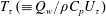
The computational domain size (
 $L_{x}\times L_{y}\times L_{z}$
), number of grid points (
$L_{x}\times L_{y}\times L_{z}$
), number of grid points (
 $N_{x}\times N_{y}\times N_{z}$
) and spatial resolution (
$N_{x}\times N_{y}\times N_{z}$
) and spatial resolution (
 $\unicode[STIX]{x0394}x$
,
$\unicode[STIX]{x0394}x$
,
 $\unicode[STIX]{x0394}y$
,
$\unicode[STIX]{x0394}y$
,
 $\unicode[STIX]{x0394}z$
) are given in table 1, the superscript * representing normalization by either
$\unicode[STIX]{x0394}z$
) are given in table 1, the superscript * representing normalization by either
 $v_{K}$
(
$v_{K}$
(
 $\equiv$
(
$\equiv$
(
 $\unicode[STIX]{x1D708}\overline{\unicode[STIX]{x1D700}}$
)
$\unicode[STIX]{x1D708}\overline{\unicode[STIX]{x1D700}}$
)
 $^{1/4}$
; the Kolmogorov velocity scale) or
$^{1/4}$
; the Kolmogorov velocity scale) or
 $\unicode[STIX]{x1D702}$
(
$\unicode[STIX]{x1D702}$
(
 $\equiv$
(
$\equiv$
(
 $\unicode[STIX]{x1D708}^{3}/\overline{\unicode[STIX]{x1D700}}$
)
$\unicode[STIX]{x1D708}^{3}/\overline{\unicode[STIX]{x1D700}}$
)
 $^{1/4}$
; the Kolmogorov length scale); the subscripts
$^{1/4}$
; the Kolmogorov length scale); the subscripts
 $w$
and
$w$
and
 $c$
referring to the wall and centreline, respectively. The effect of the domain size was examined by Abe, Kawamura & Choi (Reference Abe, Kawamura and Choi2004b
) (
$c$
referring to the wall and centreline, respectively. The effect of the domain size was examined by Abe, Kawamura & Choi (Reference Abe, Kawamura and Choi2004b
) (
 $h^{+}=640$
) who compared two cases:
$h^{+}=640$
) who compared two cases:
 $(L_{x}\times L_{z})=(6.4h\times 2h)$
and (
$(L_{x}\times L_{z})=(6.4h\times 2h)$
and (
 $12.8h\times 6.4h$
). They found that the effect on the mean flow variables and second-order moments was negligible. Abe & Antonia (Reference Abe and Antonia2016) also examined possible effects of the streamwise domain size
$12.8h\times 6.4h$
). They found that the effect on the mean flow variables and second-order moments was negligible. Abe & Antonia (Reference Abe and Antonia2016) also examined possible effects of the streamwise domain size
 $L_{x}$
on the total dissipation function
$L_{x}$
on the total dissipation function
 $E$
. They noted that while a relatively long channel is required for the experiment to achieve a fully developed flow condition (i.e.
$E$
. They noted that while a relatively long channel is required for the experiment to achieve a fully developed flow condition (i.e.
 $\text{d}\bar{P}/\text{d}x=\text{const.}$
) (Monty (Reference Monty2005) suggests
$\text{d}\bar{P}/\text{d}x=\text{const.}$
) (Monty (Reference Monty2005) suggests
 $L$
$L$
 $=260h$
), the accurate determination of
$=260h$
), the accurate determination of
 $\unicode[STIX]{x1D70F}_{w}$
in the DNS requires the channel length to be
$\unicode[STIX]{x1D70F}_{w}$
in the DNS requires the channel length to be
 $L_{x}\geqslant 2\unicode[STIX]{x03C0}h$
, which supports the finding of Lozano-Durán & Jiménez (Reference Lozano-Durán and Jiménez2014) that
$L_{x}\geqslant 2\unicode[STIX]{x03C0}h$
, which supports the finding of Lozano-Durán & Jiménez (Reference Lozano-Durán and Jiménez2014) that
 $L_{z}=2\unicode[STIX]{x03C0}h$
is sufficient to obtain good one-point statistics up to the centre of the channel.
$L_{z}=2\unicode[STIX]{x03C0}h$
is sufficient to obtain good one-point statistics up to the centre of the channel.
Table 1. Domain size, grid points and spatial resolution of the DNS databases. Constant heat lux case covers
 $h^{+}=180{-}1020$
, whereas constant heating source case covers
$h^{+}=180{-}1020$
, whereas constant heating source case covers
 $h^{+}=180$
–640.
$h^{+}=180$
–640.
Since the degree of similarity/dissimilarity between CHF and CHS is yet to be addressed in detail, we examine this issue in § 4.1 on the main quantities of interest, viz. those which contribute mostly to
 $E_{s}$
. This will be done by comparing the present simulations with the two thermal boundary conditions for
$E_{s}$
. This will be done by comparing the present simulations with the two thermal boundary conditions for
 $h^{+}=180$
, 395 and 640. Note that we run simulations with two different thermal boundary conditions simultaneously with the same domain size, number of grid points and spatial resolutions listed in table 1.
$h^{+}=180$
, 395 and 640. Note that we run simulations with two different thermal boundary conditions simultaneously with the same domain size, number of grid points and spatial resolutions listed in table 1.
4 Results for the scalar dissipation function and heat transfer coefficient
4.1 Constant heat flux versus constant heating source
We first examine the degree of similarity between CHF and CHS on quantities associated with
 $E_{s}$
. Figure 1 shows distributions of the normalized mean scalar
$E_{s}$
. Figure 1 shows distributions of the normalized mean scalar
 $\overline{\unicode[STIX]{x1D6E9}}/T_{\unicode[STIX]{x1D70F}}$
(or equivalently
$\overline{\unicode[STIX]{x1D6E9}}/T_{\unicode[STIX]{x1D70F}}$
(or equivalently
 $\overline{\unicode[STIX]{x1D6E9}}^{+}$
), the dissipation associated with the mean scalar
$\overline{\unicode[STIX]{x1D6E9}}^{+}$
), the dissipation associated with the mean scalar
 $a(\text{d}\overline{\unicode[STIX]{x1D6E9}}/\text{d}y)^{2}$
 $\unicode[STIX]{x1D708}/U_{\unicode[STIX]{x1D70F}}^{2}T_{\unicode[STIX]{x1D70F}}^{2}$
(or equivalently
$\unicode[STIX]{x1D708}/U_{\unicode[STIX]{x1D70F}}^{2}T_{\unicode[STIX]{x1D70F}}^{2}$
(or equivalently
 $(\text{d}\overline{\unicode[STIX]{x1D6E9}}^{+}/\text{d}y^{+})^{2}/Pr$
), the wall-normal turbulent heat flux
$(\text{d}\overline{\unicode[STIX]{x1D6E9}}^{+}/\text{d}y^{+})^{2}/Pr$
), the wall-normal turbulent heat flux
 $-\overline{v\unicode[STIX]{x1D703}}/U_{\unicode[STIX]{x1D70F}}T_{\unicode[STIX]{x1D70F}}$
(or equivalently
$-\overline{v\unicode[STIX]{x1D703}}/U_{\unicode[STIX]{x1D70F}}T_{\unicode[STIX]{x1D70F}}$
(or equivalently
 $-\overline{v^{+}\unicode[STIX]{x1D703}^{+}}$
) and the production term
$-\overline{v^{+}\unicode[STIX]{x1D703}^{+}}$
) and the production term
 $P_{\unicode[STIX]{x1D703}}\unicode[STIX]{x1D708}/U_{\unicode[STIX]{x1D70F}}^{2}T_{\unicode[STIX]{x1D70F}}^{2}$
(or equivalently
$P_{\unicode[STIX]{x1D703}}\unicode[STIX]{x1D708}/U_{\unicode[STIX]{x1D70F}}^{2}T_{\unicode[STIX]{x1D70F}}^{2}$
(or equivalently
 $P_{\unicode[STIX]{x1D703}}^{+}$
) for
$P_{\unicode[STIX]{x1D703}}^{+}$
) for
 $Pr=0.71$
. In figure 1(a), the empirical relation of Kader (Reference Kader1981) is also plotted. While the logarithmic law
$Pr=0.71$
. In figure 1(a), the empirical relation of Kader (Reference Kader1981) is also plotted. While the logarithmic law
 $$\begin{eqnarray}\overline{\unicode[STIX]{x1D6E9}}^{+}=\frac{1}{\unicode[STIX]{x1D705}_{\unicode[STIX]{x1D703}}}\ln y^{+}+A_{\unicode[STIX]{x1D703}}\end{eqnarray}$$
with a von Kármán constant for the mean scalar
 $\unicode[STIX]{x1D705}_{\unicode[STIX]{x1D703}}=0.43$
and an additive constant
$\unicode[STIX]{x1D705}_{\unicode[STIX]{x1D703}}=0.43$
and an additive constant
 $A_{\unicode[STIX]{x1D703}}=3.0$
provides a good fit to the DNS data for
$A_{\unicode[STIX]{x1D703}}=3.0$
provides a good fit to the DNS data for
 $h^{+}=1020$
(see figure 1
a), the value of
$h^{+}=1020$
(see figure 1
a), the value of
 $\unicode[STIX]{x1D705}_{\unicode[STIX]{x1D703}}$
tends to increase slowly with
$\unicode[STIX]{x1D705}_{\unicode[STIX]{x1D703}}$
tends to increase slowly with
 $h^{+}$
for
$h^{+}$
for
 $h^{+}<4000$
(see also figure 12 and the more critical examination of the log law in § 4.4). The log law is most likely established for the largest
$h^{+}<4000$
(see also figure 12 and the more critical examination of the log law in § 4.4). The log law is most likely established for the largest
 $h^{+}$
(
$h^{+}$
(
 ${>}4000$
). There is also a slight difference in the magnitude of
${>}4000$
). There is also a slight difference in the magnitude of
 $\overline{\unicode[STIX]{x1D6E9}}^{+}$
between CHF and CHS. This difference is pronounced in the core region, in which the empirical relation of Kader (Reference Kader1981) is closer to
$\overline{\unicode[STIX]{x1D6E9}}^{+}$
between CHF and CHS. This difference is pronounced in the core region, in which the empirical relation of Kader (Reference Kader1981) is closer to
 $\overline{\unicode[STIX]{x1D6E9}}^{+}$
for CHF than for CHS, as noted by Pirozzoli et al. (Reference Pirozzoli, Bernardini and Orlandi2016). The magnitude of
$\overline{\unicode[STIX]{x1D6E9}}^{+}$
for CHF than for CHS, as noted by Pirozzoli et al. (Reference Pirozzoli, Bernardini and Orlandi2016). The magnitude of
 $a(\text{d}\overline{\unicode[STIX]{x1D6E9}}/\text{d}y)^{2}\unicode[STIX]{x1D708}/U_{\unicode[STIX]{x1D70F}}^{2}T_{\unicode[STIX]{x1D70F}}^{2}$
(see figure 1
b) is hence slightly greater for CHF than for CHS. The magnitude of
$a(\text{d}\overline{\unicode[STIX]{x1D6E9}}/\text{d}y)^{2}\unicode[STIX]{x1D708}/U_{\unicode[STIX]{x1D70F}}^{2}T_{\unicode[STIX]{x1D70F}}^{2}$
(see figure 1
b) is hence slightly greater for CHF than for CHS. The magnitude of
 $-\overline{v\unicode[STIX]{x1D703}}/U_{\unicode[STIX]{x1D70F}}T_{\unicode[STIX]{x1D70F}}$
is also larger for CHF than for CHS (figure 1
c). These results imply a more effective heating for CHF than for CHS. Distributions of
$-\overline{v\unicode[STIX]{x1D703}}/U_{\unicode[STIX]{x1D70F}}T_{\unicode[STIX]{x1D70F}}$
is also larger for CHF than for CHS (figure 1
c). These results imply a more effective heating for CHF than for CHS. Distributions of
 $P_{\unicode[STIX]{x1D703}}$
(i.e. the product of
$P_{\unicode[STIX]{x1D703}}$
(i.e. the product of
 $-\overline{v\unicode[STIX]{x1D703}}$
and
$-\overline{v\unicode[STIX]{x1D703}}$
and
 $\text{d}\bar{\unicode[STIX]{x1D6E9}}/\text{d}y$
) normalized by
$\text{d}\bar{\unicode[STIX]{x1D6E9}}/\text{d}y$
) normalized by
 $U_{\unicode[STIX]{x1D70F}}^{2}T_{\unicode[STIX]{x1D70F}}^{2}/\unicode[STIX]{x1D708}$
thus exhibit a discernible difference between the two thermal boundary conditions (figure 1
d). In contrast to CHS, the peak value of
$U_{\unicode[STIX]{x1D70F}}^{2}T_{\unicode[STIX]{x1D70F}}^{2}/\unicode[STIX]{x1D708}$
thus exhibit a discernible difference between the two thermal boundary conditions (figure 1
d). In contrast to CHS, the peak value of
 $P_{\unicode[STIX]{x1D703}}$
for CHF reaches the theoretical maximum value of
$P_{\unicode[STIX]{x1D703}}$
for CHF reaches the theoretical maximum value of
 $Pr/4$
when
$Pr/4$
when
 $h^{+}$
is larger than 395 (figure 1
d), i.e. the scalar field for CHF reaches a local equilibrium state at a smaller
$h^{+}$
is larger than 395 (figure 1
d), i.e. the scalar field for CHF reaches a local equilibrium state at a smaller
 $h^{+}$
than for CHS. Since
$h^{+}$
than for CHS. Since
 $\langle P_{\unicode[STIX]{x1D703}}\rangle =\langle \overline{\unicode[STIX]{x1D700}_{\unicode[STIX]{x1D703}}}\rangle$
(see (2.9)), the difference in the magnitude of
$\langle P_{\unicode[STIX]{x1D703}}\rangle =\langle \overline{\unicode[STIX]{x1D700}_{\unicode[STIX]{x1D703}}}\rangle$
(see (2.9)), the difference in the magnitude of
 $P_{\unicode[STIX]{x1D703}}$
between CHS and CHF cannot be dismissed when considering the magnitude of the total scalar dissipation rate
$P_{\unicode[STIX]{x1D703}}$
between CHS and CHF cannot be dismissed when considering the magnitude of the total scalar dissipation rate
 $E_{S}$
(see § 4.2).
$E_{S}$
(see § 4.2).

Figure 1. Distributions of
 $\overline{\unicode[STIX]{x1D6E9}}^{+}$
,
$\overline{\unicode[STIX]{x1D6E9}}^{+}$
,
 $(\text{d}\overline{\unicode[STIX]{x1D6E9}}^{+}/\text{d}y^{+})^{2}/Pr$
,
$(\text{d}\overline{\unicode[STIX]{x1D6E9}}^{+}/\text{d}y^{+})^{2}/Pr$
,
 $-\overline{v^{+}\unicode[STIX]{x1D703}^{+}}$
and
$-\overline{v^{+}\unicode[STIX]{x1D703}^{+}}$
and
 $P_{\unicode[STIX]{x1D703}}\unicode[STIX]{x1D708}/U_{\unicode[STIX]{x1D70F}}^{2}T_{\unicode[STIX]{x1D70F}}^{2}$
for
$P_{\unicode[STIX]{x1D703}}\unicode[STIX]{x1D708}/U_{\unicode[STIX]{x1D70F}}^{2}T_{\unicode[STIX]{x1D70F}}^{2}$
for
 $Pr=0.71$
: (a)
$Pr=0.71$
: (a)
 $\overline{\unicode[STIX]{x1D6E9}}^{+}$
; (b)
$\overline{\unicode[STIX]{x1D6E9}}^{+}$
; (b)
 $(\text{d}\overline{\unicode[STIX]{x1D6E9}}^{+}/\text{d}y^{+})^{2}/Pr$
; (c)
$(\text{d}\overline{\unicode[STIX]{x1D6E9}}^{+}/\text{d}y^{+})^{2}/Pr$
; (c)
 $-\overline{v^{+}\unicode[STIX]{x1D703}^{+}}$
; (d)
$-\overline{v^{+}\unicode[STIX]{x1D703}^{+}}$
; (d)
 $P_{\unicode[STIX]{x1D703}}\unicode[STIX]{x1D708}/U_{\unicode[STIX]{x1D70F}}^{2}T_{\unicode[STIX]{x1D70F}}^{2}$
.
$P_{\unicode[STIX]{x1D703}}\unicode[STIX]{x1D708}/U_{\unicode[STIX]{x1D70F}}^{2}T_{\unicode[STIX]{x1D70F}}^{2}$
.

Figure 2. Quadrant analysis of
 $\overline{v\unicode[STIX]{x1D703}}$
, its probability
$\overline{v\unicode[STIX]{x1D703}}$
, its probability
 $P_{j}$
and distributions of
$P_{j}$
and distributions of
 $\mathit{Pr}_{t}$
,
$\mathit{Pr}_{t}$
,
 $(\text{d}\overline{U}/\text{d}y)/(\text{d}\overline{\unicode[STIX]{x1D6E9}}/\text{d}y)$
and
$(\text{d}\overline{U}/\text{d}y)/(\text{d}\overline{\unicode[STIX]{x1D6E9}}/\text{d}y)$
and
 $\overline{uv}/\overline{v\unicode[STIX]{x1D703}}$
for
$\overline{uv}/\overline{v\unicode[STIX]{x1D703}}$
for
 $Pr=0.71$
as a function of
$Pr=0.71$
as a function of
 $y$
/
$y$
/
 $h$
: (a)
$h$
: (a)
 $(\overline{v\unicode[STIX]{x1D703}})_{j}/(\overline{v\unicode[STIX]{x1D703}})$
; (b)
$(\overline{v\unicode[STIX]{x1D703}})_{j}/(\overline{v\unicode[STIX]{x1D703}})$
; (b)
 $P_{j}$
; (c)
$P_{j}$
; (c)
 $\mathit{Pr}_{t}$
; (d)
$\mathit{Pr}_{t}$
; (d)
 $(\text{d}\overline{U}/\text{d}y)/(\text{d}\overline{\unicode[STIX]{x1D6E9}}/\text{d}y)$
and
$(\text{d}\overline{U}/\text{d}y)/(\text{d}\overline{\unicode[STIX]{x1D6E9}}/\text{d}y)$
and
 $\overline{uv}/\overline{v\unicode[STIX]{x1D703}}$
.
$\overline{uv}/\overline{v\unicode[STIX]{x1D703}}$
.
Whilst the two heating conditions lead to different magnitudes of mean and turbulent scalar quantities when normalized by either the wall heat flux
 $Q_{w}$
or the friction temperature
$Q_{w}$
or the friction temperature
 $T_{\unicode[STIX]{x1D70F}}$
, the underlying turbulent scalar transport mechanism is essentially the same for CHS and CHF (see figure 2
a,b which show the quadrant analysis of
$T_{\unicode[STIX]{x1D70F}}$
, the underlying turbulent scalar transport mechanism is essentially the same for CHS and CHF (see figure 2
a,b which show the quadrant analysis of
 $\overline{v\unicode[STIX]{x1D703}}$
and its probability for
$\overline{v\unicode[STIX]{x1D703}}$
and its probability for
 $h^{+}=640$
). The turbulent Prandtl number
$h^{+}=640$
). The turbulent Prandtl number
 $\mathit{Pr}_{t}$
defined as the ratio of turbulent eddy viscosity
$\mathit{Pr}_{t}$
defined as the ratio of turbulent eddy viscosity
 $\unicode[STIX]{x1D708}_{t}$
(
$\unicode[STIX]{x1D708}_{t}$
(
 $\equiv \overline{uv}/\text{d}\overline{U}/\text{d}y$
) to turbulent eddy diffusivity
$\equiv \overline{uv}/\text{d}\overline{U}/\text{d}y$
) to turbulent eddy diffusivity
 $a_{t}$
(
$a_{t}$
(
 $\equiv \overline{v\unicode[STIX]{x1D703}}/\text{d}\overline{\unicode[STIX]{x1D6E9}}/\text{d}y$
), viz.
$\equiv \overline{v\unicode[STIX]{x1D703}}/\text{d}\overline{\unicode[STIX]{x1D6E9}}/\text{d}y$
), viz.
 $$\begin{eqnarray}Pr_{t}=\frac{\unicode[STIX]{x1D708}_{t}}{a_{t}}=\frac{\overline{uv}}{\overline{v\unicode[STIX]{x1D703}}}\frac{\text{d}\overline{\unicode[STIX]{x1D6E9}}/\text{d}y}{\text{d}\overline{U}/\text{d}y},\end{eqnarray}$$
is also identical for the two isothermal boundary conditions (see figure 2
c). For
 $y/h>0.2$
, the distributions of
$y/h>0.2$
, the distributions of
 $\mathit{Pr}_{t}$
are described approximately by
$\mathit{Pr}_{t}$
are described approximately by
 $$\begin{eqnarray}\mathit{Pr}_{t}=0.9{-}0.3(y/h)^{2}\end{eqnarray}$$
(Abe & Antonia Reference Abe, Antonia, Kasagi, Eaton, Friedrich, Humphrey, Johansson and Sung2009), which is analogous to the relation proposed by Rotta (Reference Rotta1962) in a turbulent boundary layer (see also Simpson, Whitten & Moffat Reference Simpson, Whitten and Moffat1970). Other DNS data (Kozuka, Seki & Kawamura Reference Kozuka, Seki and Kawamura2009) also indicate that (4.3) seems to apply not only for air but also for water (viz.
 $Pr=5$
–7). In the logarithmic region and the lower part of the outer region (
$Pr=5$
–7). In the logarithmic region and the lower part of the outer region (
 $y^{+}>100$
and
$y^{+}>100$
and
 $y/h<0.4$
),
$y/h<0.4$
),
 $\mathit{Pr}_{t}$
is nearly constant (about 0.85), where the magnitudes of
$\mathit{Pr}_{t}$
is nearly constant (about 0.85), where the magnitudes of
 $\unicode[STIX]{x1D708}_{t}/U_{\unicode[STIX]{x1D70F}}h$
and
$\unicode[STIX]{x1D708}_{t}/U_{\unicode[STIX]{x1D70F}}h$
and
 $a_{t}/U_{\unicode[STIX]{x1D70F}}h$
, which are important measures of the momentum transport and scalar transport respectively, increase monotonically (the distributions of
$a_{t}/U_{\unicode[STIX]{x1D70F}}h$
, which are important measures of the momentum transport and scalar transport respectively, increase monotonically (the distributions of
 $\unicode[STIX]{x1D708}_{t}/U_{\unicode[STIX]{x1D70F}}h$
and
$\unicode[STIX]{x1D708}_{t}/U_{\unicode[STIX]{x1D70F}}h$
and
 $a_{t}/U_{\unicode[STIX]{x1D70F}}h$
are not shown here) and they are in the range
$a_{t}/U_{\unicode[STIX]{x1D70F}}h$
are not shown here) and they are in the range
 $\unicode[STIX]{x1D708}_{t}/U_{\unicode[STIX]{x1D70F}}h=0.06$
–0.08 and
$\unicode[STIX]{x1D708}_{t}/U_{\unicode[STIX]{x1D70F}}h=0.06$
–0.08 and
 $a_{t}/U_{\unicode[STIX]{x1D70F}}h=0.08$
–0.1 (the Prandtl number dependence is negligibly small when Pr is not far from unity (see Kim & Moin Reference Kim, Moin, André, Cousteix, Durst, Launder, Schmidt and Whitelaw1989)). The latter two values agree reasonably well with model constants of the two-equation model (i.e.
$a_{t}/U_{\unicode[STIX]{x1D70F}}h=0.08$
–0.1 (the Prandtl number dependence is negligibly small when Pr is not far from unity (see Kim & Moin Reference Kim, Moin, André, Cousteix, Durst, Launder, Schmidt and Whitelaw1989)). The latter two values agree reasonably well with model constants of the two-equation model (i.e.
 $C_{\unicode[STIX]{x1D707}}$
and
$C_{\unicode[STIX]{x1D707}}$
and
 $C_{\unicode[STIX]{x1D706}}$
) proposed by Nagano & Kim (Reference Nagano and Kim1988). For
$C_{\unicode[STIX]{x1D706}}$
) proposed by Nagano & Kim (Reference Nagano and Kim1988). For
 $y/h>0.4$
, the magnitude of
$y/h>0.4$
, the magnitude of
 $\mathit{Pr}_{t}$
decreases gradually to approximately 0.6 at the channel centreline. This is most likely due to the mean scalar gradient being smaller than the mean velocity gradient (see figure 2
d). In this context, for a DNS with a constant temperature difference (i.e. both isothermal walls are either heated or cooled, so that there is a constant difference in mean temperature between the two walls) (Lyons, Hanratty & Mclaughlin Reference Lyons, Hanratty and McLaughlin1991; Seki, Abe & Kawamura Reference Seki, Abe and Kawamura2003), the largest mean scalar gradient occurs at the centreline; in this case,
$\mathit{Pr}_{t}$
decreases gradually to approximately 0.6 at the channel centreline. This is most likely due to the mean scalar gradient being smaller than the mean velocity gradient (see figure 2
d). In this context, for a DNS with a constant temperature difference (i.e. both isothermal walls are either heated or cooled, so that there is a constant difference in mean temperature between the two walls) (Lyons, Hanratty & Mclaughlin Reference Lyons, Hanratty and McLaughlin1991; Seki, Abe & Kawamura Reference Seki, Abe and Kawamura2003), the largest mean scalar gradient occurs at the centreline; in this case,
 $\mathit{Pr}_{t}$
increases towards the channel centre. The importance of the mean scalar gradient was also suggested for homogeneous shear flows by Rogers, Mansour & Reynolds (Reference Rogers, Mansour and Reynolds1989). They showed that the magnitude of
$\mathit{Pr}_{t}$
increases towards the channel centre. The importance of the mean scalar gradient was also suggested for homogeneous shear flows by Rogers, Mansour & Reynolds (Reference Rogers, Mansour and Reynolds1989). They showed that the magnitude of
 $\mathit{Pr}_{t}$
increases when the alignment between the turbulent heat flux and mean scalar gradient is perfect. The implication of the present results is that, like the similarity between
q
(the fluctuating velocity vector) and
$\mathit{Pr}_{t}$
increases when the alignment between the turbulent heat flux and mean scalar gradient is perfect. The implication of the present results is that, like the similarity between
q
(the fluctuating velocity vector) and
 $\unicode[STIX]{x1D703}$
(see Antonia et al. (Reference Antonia, Abe and Kawamura2009)), the presence of a source (production) term is an important ingredient for a close analogy between the velocity and scalar transport. The difference in magnitude between
$\unicode[STIX]{x1D703}$
(see Antonia et al. (Reference Antonia, Abe and Kawamura2009)), the presence of a source (production) term is an important ingredient for a close analogy between the velocity and scalar transport. The difference in magnitude between
 $\text{d}\overline{U}/\text{d}y$
and
$\text{d}\overline{U}/\text{d}y$
and
 $\text{d}\bar{\unicode[STIX]{x1D6E9}}/\text{d}y$
will also be discussed in § 4.4 in the context of the von Kármán constants
$\text{d}\bar{\unicode[STIX]{x1D6E9}}/\text{d}y$
will also be discussed in § 4.4 in the context of the von Kármán constants
 $\unicode[STIX]{x1D705}$
and
$\unicode[STIX]{x1D705}$
and
 $\unicode[STIX]{x1D705}_{\unicode[STIX]{x1D703}}$
.
$\unicode[STIX]{x1D705}_{\unicode[STIX]{x1D703}}$
.
Note that the decreasing magnitude of
 $\mathit{Pr}_{t}$
is essentially associated with the unmixedness of the scalar (Guezennec, Stretch & Kim Reference Guezennec, Stretch and Kim1990; Antonia et al.
Reference Antonia, Abe and Kawamura2009; Pirozzoli et al.
Reference Pirozzoli, Bernardini and Orlandi2016). Here, close inspection of instantaneous fields has further revealed that negative regions of
$\mathit{Pr}_{t}$
is essentially associated with the unmixedness of the scalar (Guezennec, Stretch & Kim Reference Guezennec, Stretch and Kim1990; Antonia et al.
Reference Antonia, Abe and Kawamura2009; Pirozzoli et al.
Reference Pirozzoli, Bernardini and Orlandi2016). Here, close inspection of instantaneous fields has further revealed that negative regions of
 $\unicode[STIX]{x1D703}$
are more significantly transported than those of
$\unicode[STIX]{x1D703}$
are more significantly transported than those of
 $u$
by vortical motions in the outer region (see also the relationship between the vorticity and scalar derivative vectors in Abe et al. (Reference Abe, Antonia and Kawamura2009)), leading to an increased dissimilarity between velocity and scalar transports (see, for example,
$u$
by vortical motions in the outer region (see also the relationship between the vorticity and scalar derivative vectors in Abe et al. (Reference Abe, Antonia and Kawamura2009)), leading to an increased dissimilarity between velocity and scalar transports (see, for example,
 $y/h\approx 0.8$
and
$y/h\approx 0.8$
and
 $z/h\approx 1.5$
in figure 3). In the latter context, Djenidi & Antonia (Reference Djenidi and Antonia2009) also noted that, for a three-dimensional transitional wake of a heated square cylinder, the passive scalar is more effectively transported by vortical motions than momentum except close to the cylinder where the magnitudes of the mean velocity and scalar gradients are large. The enhanced scalar transport by vortical motions is most likely responsible for the decrease of
$z/h\approx 1.5$
in figure 3). In the latter context, Djenidi & Antonia (Reference Djenidi and Antonia2009) also noted that, for a three-dimensional transitional wake of a heated square cylinder, the passive scalar is more effectively transported by vortical motions than momentum except close to the cylinder where the magnitudes of the mean velocity and scalar gradients are large. The enhanced scalar transport by vortical motions is most likely responsible for the decrease of
 $\mathit{Pr}_{t}$
towards the centreline. This may also explain the difference in scaling behaviours between
$\mathit{Pr}_{t}$
towards the centreline. This may also explain the difference in scaling behaviours between
 $\overline{uu}$
and
$\overline{uu}$
and
 $\overline{\unicode[STIX]{x1D703}\unicode[STIX]{x1D703}}$
; the collapse of
$\overline{\unicode[STIX]{x1D703}\unicode[STIX]{x1D703}}$
; the collapse of
 $\overline{\unicode[STIX]{x1D703}\unicode[STIX]{x1D703}}/T_{\unicode[STIX]{x1D70F}}^{2}$
is more convincing than that of
$\overline{\unicode[STIX]{x1D703}\unicode[STIX]{x1D703}}/T_{\unicode[STIX]{x1D70F}}^{2}$
is more convincing than that of
 $\overline{uu}/U_{\unicode[STIX]{x1D70F}}^{2}$
in the outer region (Pirozzoli et al.
Reference Pirozzoli, Bernardini and Orlandi2016) where a mixed scaling, or normalization by
$\overline{uu}/U_{\unicode[STIX]{x1D70F}}^{2}$
in the outer region (Pirozzoli et al.
Reference Pirozzoli, Bernardini and Orlandi2016) where a mixed scaling, or normalization by
 $U_{\unicode[STIX]{x1D70F}}U_{0}$
(
$U_{\unicode[STIX]{x1D70F}}U_{0}$
(
 $U_{0}$
is the mean centreline velocity), seems to yield an adequate collapse for
$U_{0}$
is the mean centreline velocity), seems to yield an adequate collapse for
 $\overline{uu}$
(Bernardini, Pirozzoli & Orlandi Reference Bernardini, Pirozzoli and Orlandi2014).
$\overline{uu}$
(Bernardini, Pirozzoli & Orlandi Reference Bernardini, Pirozzoli and Orlandi2014).

Figure 3. Instantaneous isocontours in the
 $y$
–
$y$
–
 $z$
plane of the streamwise velocity and scalar fluctuations for
$z$
plane of the streamwise velocity and scalar fluctuations for
 $h^{+}=1020$
: (a)
$h^{+}=1020$
: (a)
 $u^{+}$
; (b)
$u^{+}$
; (b)
 $\unicode[STIX]{x1D703}^{+}$
for
$\unicode[STIX]{x1D703}^{+}$
for
 $Pr=0.71$
(CHF). Lines denote the positive values of the second invariant of the velocity gradient tensor
$Pr=0.71$
(CHF). Lines denote the positive values of the second invariant of the velocity gradient tensor
 $Q^{+}$
(line contour levels are from
$Q^{+}$
(line contour levels are from
 $5\times 10^{-4}$
to
$5\times 10^{-4}$
to
 $5\times 10^{-3}$
with an increment of
$5\times 10^{-3}$
with an increment of
 $5\times 10^{-5}$
).
$5\times 10^{-5}$
).
4.2 Scalar integrals and their Reynolds number dependence
Next, attention is given to the
 $h^{+}$
dependence of the total scalar dissipation function
$h^{+}$
dependence of the total scalar dissipation function
 $E_{S}/U_{\unicode[STIX]{x1D70F}}T_{\unicode[STIX]{x1D70F}}^{2}$
, hence
$E_{S}/U_{\unicode[STIX]{x1D70F}}T_{\unicode[STIX]{x1D70F}}^{2}$
, hence
 $T_{m}^{+}$
for CHF (2.13) or
$T_{m}^{+}$
for CHF (2.13) or
 $T_{b}^{+}$
for CHS (2.12). Distributions of
$T_{b}^{+}$
for CHS (2.12). Distributions of
 $T_{m}$
and
$T_{m}$
and
 $T_{b}$
, normalized by
$T_{b}$
, normalized by
 $T_{\unicode[STIX]{x1D70F}}$
are given in figures 4(a) and (b), respectively, as a function of
$T_{\unicode[STIX]{x1D70F}}$
are given in figures 4(a) and (b), respectively, as a function of
 $h^{+}$
. Clearly, the magnitudes of both
$h^{+}$
. Clearly, the magnitudes of both
 $T_{m}^{+}$
and
$T_{m}^{+}$
and
 $T_{b}^{+}$
increase logarithmically with increasing
$T_{b}^{+}$
increase logarithmically with increasing
 $h^{+}$
when
$h^{+}$
when
 $h^{+}$
exceeds 400. This increase is described well by
$h^{+}$
exceeds 400. This increase is described well by
 $$\begin{eqnarray}T_{m}^{+}=2.18\ln (h^{+})+2.40\end{eqnarray}$$
and
 $$\begin{eqnarray}T_{b}^{+}=2.18\ln (h^{+})+1.30\end{eqnarray}$$
for CHF and CHS, respectively. While the slope for
 $T_{m}^{+}$
(4.4) is close to that obtained by Kader & Yaglom (Reference Kader and Yaglom1972) for a pipe flow (see figure 4(a) where the CHF pipe data of Ould-Rouiss, Bousbai & Mazouz (Reference Ould-Rouiss, Bousbai and Mazouz2013) are also plotted), the intercept is somewhat smaller than for the channel. Figure 4 underlines that the slope of 2.18 is intrinsically the same between the two thermal boundary conditions, whilst it is smaller than that (2.54) for
$T_{m}^{+}$
(4.4) is close to that obtained by Kader & Yaglom (Reference Kader and Yaglom1972) for a pipe flow (see figure 4(a) where the CHF pipe data of Ould-Rouiss, Bousbai & Mazouz (Reference Ould-Rouiss, Bousbai and Mazouz2013) are also plotted), the intercept is somewhat smaller than for the channel. Figure 4 underlines that the slope of 2.18 is intrinsically the same between the two thermal boundary conditions, whilst it is smaller than that (2.54) for
 $U_{b}^{+}$
(see also (1.14)). The resulting Reynolds analogy factor
$U_{b}^{+}$
(see also (1.14)). The resulting Reynolds analogy factor
 $2h_{t}/C_{f}=U_{b}^{+}/\unicode[STIX]{x1D703}_{b}^{+}\,\,or\,\,U_{b}^{+}/\unicode[STIX]{x1D703}_{m}^{+}$
is approximately 1.2 for
$2h_{t}/C_{f}=U_{b}^{+}/\unicode[STIX]{x1D703}_{b}^{+}\,\,or\,\,U_{b}^{+}/\unicode[STIX]{x1D703}_{m}^{+}$
is approximately 1.2 for
 $h^{+}\approx 500$
. Nearly the same value was obtained in a thermal boundary layer with air at low Reynolds number (Kong, Choi & Lee Reference Kong, Choi and Lee2000; Li et al.
Reference Li, Schlatter, Brandt and Henningson2009). The magnitude of
$h^{+}\approx 500$
. Nearly the same value was obtained in a thermal boundary layer with air at low Reynolds number (Kong, Choi & Lee Reference Kong, Choi and Lee2000; Li et al.
Reference Li, Schlatter, Brandt and Henningson2009). The magnitude of
 $2h_{t}/C_{f}$
however tends to increase slowly with
$2h_{t}/C_{f}$
however tends to increase slowly with
 $h^{+}$
. To clarify the possible Pr effect, we have included the available DNS data for
$h^{+}$
. To clarify the possible Pr effect, we have included the available DNS data for
 $Pr=1$
(Hasegawa & Kasagi Reference Hasegawa and Kasagi2011; Pirozzoli et al.
Reference Pirozzoli, Bernardini and Orlandi2016) in figure 4(b). Whilst the magnitude of
$Pr=1$
(Hasegawa & Kasagi Reference Hasegawa and Kasagi2011; Pirozzoli et al.
Reference Pirozzoli, Bernardini and Orlandi2016) in figure 4(b). Whilst the magnitude of
 $2h_{t}/C_{f}$
becomes closer to unity for
$2h_{t}/C_{f}$
becomes closer to unity for
 $Pr=1$
at low Reynolds number, the slope remains invariably unchanged so that the difference becomes increasingly pronounced with
$Pr=1$
at low Reynolds number, the slope remains invariably unchanged so that the difference becomes increasingly pronounced with
 $h^{+}$
. We infer that the difference in slope between
$h^{+}$
. We infer that the difference in slope between
 $U_{b}^{+}$
and
$U_{b}^{+}$
and
 $T_{b}^{+}$
(or
$T_{b}^{+}$
(or
 $T_{m}^{+}$
) is associated with different characteristics in the overlap region between velocity and scalar fields, as will be seen below.
$T_{m}^{+}$
) is associated with different characteristics in the overlap region between velocity and scalar fields, as will be seen below.

Figure 4. Distributions of
 $T_{m}^{+}$
and
$T_{m}^{+}$
and
 $T_{b}^{+}$
for
$T_{b}^{+}$
for
 $Pr=0.71$
as a function of
$Pr=0.71$
as a function of
 $h^{+}$
: (a)
$h^{+}$
: (a)
 $T_{m}^{+}$
; (b)
$T_{m}^{+}$
; (b)
 $T_{b}^{+}$
.
$T_{b}^{+}$
.
Figure 5 demonstrates that the relative contributions of the normalized values of
 $\langle \overline{\unicode[STIX]{x1D700}_{\unicode[STIX]{x1D703}}}\rangle$
(or equivalently
$\langle \overline{\unicode[STIX]{x1D700}_{\unicode[STIX]{x1D703}}}\rangle$
(or equivalently
 $\langle P_{\unicode[STIX]{x1D703}}\rangle$
) and
$\langle P_{\unicode[STIX]{x1D703}}\rangle$
) and
 $\langle a(\text{d}\bar{\unicode[STIX]{x1D6E9}}/\text{d}y)^{2}\rangle$
to
$\langle a(\text{d}\bar{\unicode[STIX]{x1D6E9}}/\text{d}y)^{2}\rangle$
to
 $T_{m}^{+}$
(2.13) and
$T_{m}^{+}$
(2.13) and
 $T_{b}^{+}$
(2.12). Clearly, the magnitude of
$T_{b}^{+}$
(2.12). Clearly, the magnitude of
 $\langle \overline{\unicode[STIX]{x1D700}_{\unicode[STIX]{x1D703}}}\rangle /U_{\unicode[STIX]{x1D70F}}T_{\unicode[STIX]{x1D70F}}^{2}$
increases logarithmically with increasing
$\langle \overline{\unicode[STIX]{x1D700}_{\unicode[STIX]{x1D703}}}\rangle /U_{\unicode[STIX]{x1D70F}}T_{\unicode[STIX]{x1D70F}}^{2}$
increases logarithmically with increasing
 $h^{+}$
(figure 5
a), while that of
$h^{+}$
(figure 5
a), while that of
 $\langle a(\text{d}\bar{\unicode[STIX]{x1D6E9}}/\text{d}y)^{2}\rangle /U_{\unicode[STIX]{x1D70F}}T_{\unicode[STIX]{x1D70F}}^{2}$
is approximately constant (
$\langle a(\text{d}\bar{\unicode[STIX]{x1D6E9}}/\text{d}y)^{2}\rangle /U_{\unicode[STIX]{x1D70F}}T_{\unicode[STIX]{x1D70F}}^{2}$
is approximately constant (
 ${\approx}$
7.6 and 7.4 for CHF and CHS, respectively) for
${\approx}$
7.6 and 7.4 for CHF and CHS, respectively) for
 $h^{+}\geqslant 400$
(figure 5
b). As for
$h^{+}\geqslant 400$
(figure 5
b). As for
 $\langle \overline{\unicode[STIX]{x1D700}}\rangle /U_{\unicode[STIX]{x1D70F}}^{3}$
(see figure 3
b of Abe & Antonia (Reference Abe and Antonia2016)), the logarithmic
$\langle \overline{\unicode[STIX]{x1D700}}\rangle /U_{\unicode[STIX]{x1D70F}}^{3}$
(see figure 3
b of Abe & Antonia (Reference Abe and Antonia2016)), the logarithmic
 $h^{+}$
increase for
$h^{+}$
increase for
 $\langle \overline{\unicode[STIX]{x1D700}_{\unicode[STIX]{x1D703}}}\rangle /U_{\unicode[STIX]{x1D70F}}T_{\unicode[STIX]{x1D70F}}^{2}$
is established even at small
$\langle \overline{\unicode[STIX]{x1D700}_{\unicode[STIX]{x1D703}}}\rangle /U_{\unicode[STIX]{x1D70F}}T_{\unicode[STIX]{x1D70F}}^{2}$
is established even at small
 $h^{+}$
(i.e.
$h^{+}$
(i.e.
 $h^{+}\geqslant 400$
), which is much lower than the Reynolds number for which the mean temperature log law holds. The latter reason is essentially associated with the overlap region of the mean turbulent scalar dissipation rate
$h^{+}\geqslant 400$
), which is much lower than the Reynolds number for which the mean temperature log law holds. The latter reason is essentially associated with the overlap region of the mean turbulent scalar dissipation rate
 $\overline{\unicode[STIX]{x1D700}_{\unicode[STIX]{x1D703}}}$
(see § 4.3). The logarithmic
$\overline{\unicode[STIX]{x1D700}_{\unicode[STIX]{x1D703}}}$
(see § 4.3). The logarithmic
 $h^{+}$
dependence of
$h^{+}$
dependence of
 $\langle \overline{\unicode[STIX]{x1D700}_{\unicode[STIX]{x1D703}}}\rangle /U_{\unicode[STIX]{x1D70F}}T_{\unicode[STIX]{x1D70F}}^{2}$
is represented well by
$\langle \overline{\unicode[STIX]{x1D700}_{\unicode[STIX]{x1D703}}}\rangle /U_{\unicode[STIX]{x1D70F}}T_{\unicode[STIX]{x1D70F}}^{2}$
is represented well by
 $$\begin{eqnarray}\langle \overline{\unicode[STIX]{x1D700}_{\unicode[STIX]{x1D703}}}\rangle /U_{\unicode[STIX]{x1D70F}}T_{\unicode[STIX]{x1D70F}}^{2}=2.18\ln (h^{+})-C_{\unicode[STIX]{x1D703}},\end{eqnarray}$$
with
 $C_{\unicode[STIX]{x1D703}}=5.2$
and 6.1 for CHF and CHS, respectively. Relation (4.6) was obtained by substituting the relations for
$C_{\unicode[STIX]{x1D703}}=5.2$
and 6.1 for CHF and CHS, respectively. Relation (4.6) was obtained by substituting the relations for
 $T_{m}^{+}$
(4.4) and
$T_{m}^{+}$
(4.4) and
 $T_{b}^{+}$
(4.5) and the constants (7.6 and 7.4 for CHF and CHS, respectively) of
$T_{b}^{+}$
(4.5) and the constants (7.6 and 7.4 for CHF and CHS, respectively) of
 $\langle a(\text{d}\bar{\unicode[STIX]{x1D6E9}}/\text{d}y)^{2}\rangle /U_{\unicode[STIX]{x1D70F}}T_{\unicode[STIX]{x1D70F}}^{2}$
into (2.13) and (2.12). Viscosity affects
$\langle a(\text{d}\bar{\unicode[STIX]{x1D6E9}}/\text{d}y)^{2}\rangle /U_{\unicode[STIX]{x1D70F}}T_{\unicode[STIX]{x1D70F}}^{2}$
into (2.13) and (2.12). Viscosity affects
 $\langle \overline{\unicode[STIX]{x1D700}_{\unicode[STIX]{x1D703}}}\rangle$
and
$\langle \overline{\unicode[STIX]{x1D700}_{\unicode[STIX]{x1D703}}}\rangle$
and
 $\langle a(\text{d}\bar{\unicode[STIX]{x1D6E9}}/\text{d}y)^{2}\rangle$
significantly below
$\langle a(\text{d}\bar{\unicode[STIX]{x1D6E9}}/\text{d}y)^{2}\rangle$
significantly below
 $h^{+}=400$
since there is no separation between the inner and outer regions.
$h^{+}=400$
since there is no separation between the inner and outer regions.

Figure 5. Distributions of
 $\langle \overline{\unicode[STIX]{x1D700}_{\unicode[STIX]{x1D703}}}\rangle /U_{\unicode[STIX]{x1D70F}}T_{\unicode[STIX]{x1D70F}}^{2}$
and
$\langle \overline{\unicode[STIX]{x1D700}_{\unicode[STIX]{x1D703}}}\rangle /U_{\unicode[STIX]{x1D70F}}T_{\unicode[STIX]{x1D70F}}^{2}$
and
 $\langle a(\text{d}\overline{\unicode[STIX]{x1D6E9}}/\text{d}y)^{2}\rangle /U_{\unicode[STIX]{x1D70F}}T_{\unicode[STIX]{x1D70F}}^{2}$
for
$\langle a(\text{d}\overline{\unicode[STIX]{x1D6E9}}/\text{d}y)^{2}\rangle /U_{\unicode[STIX]{x1D70F}}T_{\unicode[STIX]{x1D70F}}^{2}$
for
 $Pr=0.71$
as a function of
$Pr=0.71$
as a function of
 $h^{+}$
: (a)
$h^{+}$
: (a)
 $\langle \overline{\unicode[STIX]{x1D700}_{\unicode[STIX]{x1D703}}}\rangle /U_{\unicode[STIX]{x1D70F}}T_{\unicode[STIX]{x1D70F}}^{2}$
; (b)
$\langle \overline{\unicode[STIX]{x1D700}_{\unicode[STIX]{x1D703}}}\rangle /U_{\unicode[STIX]{x1D70F}}T_{\unicode[STIX]{x1D70F}}^{2}$
; (b)
 $\langle a(\text{d}\overline{\unicode[STIX]{x1D6E9}}/\text{d}y)^{2}\rangle /U_{\unicode[STIX]{x1D70F}}T_{\unicode[STIX]{x1D70F}}^{2}$
.
$\langle a(\text{d}\overline{\unicode[STIX]{x1D6E9}}/\text{d}y)^{2}\rangle /U_{\unicode[STIX]{x1D70F}}T_{\unicode[STIX]{x1D70F}}^{2}$
.
We next discuss a possible relation for the heat transfer coefficient
 $h_{t}$
(1.1), which may readily be obtained on the basis of a global energy balance by substituting the present
$h_{t}$
(1.1), which may readily be obtained on the basis of a global energy balance by substituting the present
 $T_{m}^{+}$
relation (4.4) into (1.1), viz.
$T_{m}^{+}$
relation (4.4) into (1.1), viz.
 $$\begin{eqnarray}h_{t}=\frac{\sqrt{(C_{f}/2)}}{2.18\ln (Re_{b}\sqrt{C_{f}}/2\sqrt{2})+2.40}.\end{eqnarray}$$
Note that (4.7) is no longer analogous to (1.10), as derived by Kader & Yaglom (Reference Kader and Yaglom1972) from the log law since the latter is not assumed when obtaining (4.7). With the use of the logarithmic skin friction law (1.15), the present logarithmic heat transfer law (4.7) can then be used for evaluating the Reynolds number dependence of the Nusselt number,
 $Nu\equiv h_{t}Re_{b}Pr$
. Figure 6 shows distributions of
$Nu\equiv h_{t}Re_{b}Pr$
. Figure 6 shows distributions of
 $Nu$
for
$Nu$
for
 $Pr=0.71$
with the DNS data for both CHF and CHS in the range
$Pr=0.71$
with the DNS data for both CHF and CHS in the range
 $1.6\times 10^{3}\leqslant Re_{b}\leqslant 2.0\times 10^{5}$
(i.e.
$1.6\times 10^{3}\leqslant Re_{b}\leqslant 2.0\times 10^{5}$
(i.e.
 $60\leqslant h^{+}\leqslant 4000$
). This figure highlights that
$60\leqslant h^{+}\leqslant 4000$
). This figure highlights that
 $Nu$
obtained from both (4.7) and (1.15) gives a reasonable fit to the DNS data for CHF provided
$Nu$
obtained from both (4.7) and (1.15) gives a reasonable fit to the DNS data for CHF provided
 $Re_{b}\geqslant 6000$
(or equivalently
$Re_{b}\geqslant 6000$
(or equivalently
 $h^{+}\geqslant 200$
). On the other hand, since the constant heat flux is not guaranteed for CHS, the resulting
$h^{+}\geqslant 200$
). On the other hand, since the constant heat flux is not guaranteed for CHS, the resulting
 $Nu$
for CHS is a few per cent larger than that for CHF in the range
$Nu$
for CHS is a few per cent larger than that for CHF in the range
 $Re_{b}\geqslant 1.4\times 10^{4}$
(or equivalently
$Re_{b}\geqslant 1.4\times 10^{4}$
(or equivalently
 $h^{+}\geqslant 400$
) where
$h^{+}\geqslant 400$
) where
 $T_{m}^{+}$
also differs between the two thermal boundary conditions (see figure 4
a). There is also a discernible difference between the present prediction and the well-known empirical relation obtained by Kays & Crawford (Reference Kays and Crawford1980), i.e.
$T_{m}^{+}$
also differs between the two thermal boundary conditions (see figure 4
a). There is also a discernible difference between the present prediction and the well-known empirical relation obtained by Kays & Crawford (Reference Kays and Crawford1980), i.e.
 $$\begin{eqnarray}Nu=0.021Re_{b}^{0.8}Pr^{0.5}.\end{eqnarray}$$
This latter relation tends to overpredict the Nusselt number slightly in the range
 $Re_{b}\geqslant 1.4\times 10^{4}$
and follow the DNS data for CHS. The lower
$Re_{b}\geqslant 1.4\times 10^{4}$
and follow the DNS data for CHS. The lower
 $h^{+}$
bound of the present prediction for
$h^{+}$
bound of the present prediction for
 $Nu$
(i.e.
$Nu$
(i.e.
 $h^{+}\geqslant 200$
) is approximately a factor of 2 smaller than that for
$h^{+}\geqslant 200$
) is approximately a factor of 2 smaller than that for
 $T_{m}^{+}$
(
$T_{m}^{+}$
(
 $h^{+}\geqslant 400$
). This is most likely due to the combined effect of the bulk mean velocity
$h^{+}\geqslant 400$
). This is most likely due to the combined effect of the bulk mean velocity
 $U_{b}^{+}$
and the bulk mean scalar
$U_{b}^{+}$
and the bulk mean scalar
 $T_{m}^{+}$
in the heat transfer coefficient
$T_{m}^{+}$
in the heat transfer coefficient
 $h_{t}$
(i.e. equation (1.1)) since the logarithmic skin friction law is established on the basis of a global energy balance for
$h_{t}$
(i.e. equation (1.1)) since the logarithmic skin friction law is established on the basis of a global energy balance for
 $h^{+}\geqslant 300$
(see Abe & Antonia Reference Abe and Antonia2016).
$h^{+}\geqslant 300$
(see Abe & Antonia Reference Abe and Antonia2016).

Figure 6. Distributions of
 $Nu$
for
$Nu$
for
 $Pr=0.71$
as a function of
$Pr=0.71$
as a function of
 $Re_{b}$
. Solid line represents the present relation obtained from both (4.7) and (1.15), whereas dashed line represents the empirical relation of Kays & Crawford (Reference Kays and Crawford1980),
$Re_{b}$
. Solid line represents the present relation obtained from both (4.7) and (1.15), whereas dashed line represents the empirical relation of Kays & Crawford (Reference Kays and Crawford1980),
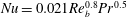 $Nu=0.021Re_{b}^{0.8}Pr^{0.5}$
.
$Nu=0.021Re_{b}^{0.8}Pr^{0.5}$
.
4.3 Scaling laws of
 $\overline{\unicode[STIX]{x1D700}_{\unicode[STIX]{x1D703}}}$
and matching argument
$\overline{\unicode[STIX]{x1D700}_{\unicode[STIX]{x1D703}}}$
and matching argument

In this subsection, we focus on the scaling of
 $\overline{\unicode[STIX]{x1D700}_{\unicode[STIX]{x1D703}}}$
for
$\overline{\unicode[STIX]{x1D700}_{\unicode[STIX]{x1D703}}}$
for
 $Pr=0.71$
in the present flow to provide further insight into the logarithmic
$Pr=0.71$
in the present flow to provide further insight into the logarithmic
 $h^{+}$
dependence of the integrated scalar dissipation
$h^{+}$
dependence of the integrated scalar dissipation
 $\langle \overline{\unicode[STIX]{x1D700}_{\unicode[STIX]{x1D703}}}\rangle /U_{\unicode[STIX]{x1D70F}}T_{\unicode[STIX]{x1D70F}}^{2}$
. The underlying idea of this analysis comes from the scaling arguments of Townsend (Reference Townsend1976) (see § 8.8 of his book). Given that the effect of Pr on
$\langle \overline{\unicode[STIX]{x1D700}_{\unicode[STIX]{x1D703}}}\rangle /U_{\unicode[STIX]{x1D70F}}T_{\unicode[STIX]{x1D70F}}^{2}$
. The underlying idea of this analysis comes from the scaling arguments of Townsend (Reference Townsend1976) (see § 8.8 of his book). Given that the effect of Pr on
 $\overline{\unicode[STIX]{x1D700}_{\unicode[STIX]{x1D703}}}$
is confined near the wall (Na, Papavassiliou & Hanratty Reference Na, Papavassiliou and Hanratty1999; Kozuka et al.
Reference Kozuka, Seki and Kawamura2009; see also figure 6
a), the inner and outer scaling laws may be written as
$\overline{\unicode[STIX]{x1D700}_{\unicode[STIX]{x1D703}}}$
is confined near the wall (Na, Papavassiliou & Hanratty Reference Na, Papavassiliou and Hanratty1999; Kozuka et al.
Reference Kozuka, Seki and Kawamura2009; see also figure 6
a), the inner and outer scaling laws may be written as
 $$\begin{eqnarray}\overline{\unicode[STIX]{x1D700}_{\unicode[STIX]{x1D703}}}^{+}\equiv \overline{\unicode[STIX]{x1D700}_{\unicode[STIX]{x1D703}}}\unicode[STIX]{x1D708}/U_{\unicode[STIX]{x1D70F}}^{2}T_{\unicode[STIX]{x1D70F}}^{2}=f(y^{+},Pr)\end{eqnarray}$$
and
 $$\begin{eqnarray}\overline{\unicode[STIX]{x1D700}_{\unicode[STIX]{x1D703}}}h/U_{\unicode[STIX]{x1D70F}}T_{\unicode[STIX]{x1D70F}}^{2}=g(y/h),\end{eqnarray}$$
respectively. While the magnitude of
 $\overline{\unicode[STIX]{x1D700}_{\unicode[STIX]{x1D703}}}^{+}$
increases with
$\overline{\unicode[STIX]{x1D700}_{\unicode[STIX]{x1D703}}}^{+}$
increases with
 $h^{+}$
close to the wall due to the effect of the inactive motion (Bradshaw Reference Bradshaw1967),
$h^{+}$
close to the wall due to the effect of the inactive motion (Bradshaw Reference Bradshaw1967),
 $\overline{\unicode[STIX]{x1D700}_{\unicode[STIX]{x1D703}}}^{+}$
seems to collapse for
$\overline{\unicode[STIX]{x1D700}_{\unicode[STIX]{x1D703}}}^{+}$
seems to collapse for
 $y^{+}\geqslant 30$
provided
$y^{+}\geqslant 30$
provided
 $h^{+}\geqslant 400$
(figure 7). Viscous effects are unlikely to affect the turbulent scalar dissipation rate significantly for
$h^{+}\geqslant 400$
(figure 7). Viscous effects are unlikely to affect the turbulent scalar dissipation rate significantly for
 $y^{+}>30$
. On the other hand,
$y^{+}>30$
. On the other hand,
 $\overline{\unicode[STIX]{x1D700}_{\unicode[STIX]{x1D703}}}$
collapses almost perfectly on
$\overline{\unicode[STIX]{x1D700}_{\unicode[STIX]{x1D703}}}$
collapses almost perfectly on
 $U_{\unicode[STIX]{x1D70F}}T_{\unicode[STIX]{x1D70F}}^{2}$
and
$U_{\unicode[STIX]{x1D70F}}T_{\unicode[STIX]{x1D70F}}^{2}$
and
 $h$
in the region
$h$
in the region
 $30/h^{+}<y/h<1$
for
$30/h^{+}<y/h<1$
for
 $h^{+}\geqslant 400$
(see figure 7
a,b). The present results highlight that the outer layer similarity is more convincing for
$h^{+}\geqslant 400$
(see figure 7
a,b). The present results highlight that the outer layer similarity is more convincing for
 $\overline{\unicode[STIX]{x1D700}_{\unicode[STIX]{x1D703}}}$
than for
$\overline{\unicode[STIX]{x1D700}_{\unicode[STIX]{x1D703}}}$
than for
 $\overline{\unicode[STIX]{x1D6E9}}$
even at small
$\overline{\unicode[STIX]{x1D6E9}}$
even at small
 $h^{+}$
(see figure 8) as was observed for
$h^{+}$
(see figure 8) as was observed for
 $\overline{\unicode[STIX]{x1D700}}$
by Abe & Antonia (Reference Abe and Antonia2016).
$\overline{\unicode[STIX]{x1D700}}$
by Abe & Antonia (Reference Abe and Antonia2016).

Figure 7. Distributions of
 $\overline{\unicode[STIX]{x1D700}_{\unicode[STIX]{x1D703}}}\unicode[STIX]{x1D708}/U_{\unicode[STIX]{x1D70F}}^{2}T_{\unicode[STIX]{x1D70F}}^{2}$
for
$\overline{\unicode[STIX]{x1D700}_{\unicode[STIX]{x1D703}}}\unicode[STIX]{x1D708}/U_{\unicode[STIX]{x1D70F}}^{2}T_{\unicode[STIX]{x1D70F}}^{2}$
for
 $Pr=0.71$
: (a) CHF; (b) CHS.
$Pr=0.71$
: (a) CHF; (b) CHS.

Figure 8. Distributions of
 $\overline{\unicode[STIX]{x1D700}_{\unicode[STIX]{x1D703}}}h/U_{\unicode[STIX]{x1D70F}}T_{\unicode[STIX]{x1D70F}}^{2}$
and
$\overline{\unicode[STIX]{x1D700}_{\unicode[STIX]{x1D703}}}h/U_{\unicode[STIX]{x1D70F}}T_{\unicode[STIX]{x1D70F}}^{2}$
and
 $(\unicode[STIX]{x1D6E9}_{0}-\overline{\unicode[STIX]{x1D6E9}})/T_{\unicode[STIX]{x1D70F}}$
for
$(\unicode[STIX]{x1D6E9}_{0}-\overline{\unicode[STIX]{x1D6E9}})/T_{\unicode[STIX]{x1D70F}}$
for
 $Pr=0.71$
as a function of
$Pr=0.71$
as a function of
 $h^{+}$
: (a)
$h^{+}$
: (a)
 $\overline{\unicode[STIX]{x1D700}_{\unicode[STIX]{x1D703}}}h/U_{\unicode[STIX]{x1D70F}}T_{\unicode[STIX]{x1D70F}}^{2}$
(CHF); (b)
$\overline{\unicode[STIX]{x1D700}_{\unicode[STIX]{x1D703}}}h/U_{\unicode[STIX]{x1D70F}}T_{\unicode[STIX]{x1D70F}}^{2}$
(CHF); (b)
 $\overline{\unicode[STIX]{x1D700}_{\unicode[STIX]{x1D703}}}h/U_{\unicode[STIX]{x1D70F}}T_{\unicode[STIX]{x1D70F}}^{2}$
(CHS); (c)
$\overline{\unicode[STIX]{x1D700}_{\unicode[STIX]{x1D703}}}h/U_{\unicode[STIX]{x1D70F}}T_{\unicode[STIX]{x1D70F}}^{2}$
(CHS); (c)
 $(\unicode[STIX]{x1D6E9}_{0}-\overline{\unicode[STIX]{x1D6E9}})/T_{\unicode[STIX]{x1D70F}}$
(CHF); (d)
$(\unicode[STIX]{x1D6E9}_{0}-\overline{\unicode[STIX]{x1D6E9}})/T_{\unicode[STIX]{x1D70F}}$
(CHF); (d)
 $(\unicode[STIX]{x1D6E9}_{0}-\overline{\unicode[STIX]{x1D6E9}})/T_{\unicode[STIX]{x1D70F}}$
(CHS).
$(\unicode[STIX]{x1D6E9}_{0}-\overline{\unicode[STIX]{x1D6E9}})/T_{\unicode[STIX]{x1D70F}}$
(CHS).
We now apply a matching argument to
 $\overline{\unicode[STIX]{x1D700}_{\unicode[STIX]{x1D703}}}$
. Here, we assume that
$\overline{\unicode[STIX]{x1D700}_{\unicode[STIX]{x1D703}}}$
. Here, we assume that
 $h^{+}$
is large enough to have a clear distinction between the inner and outer regions, and that there is a region where relations (4.9), (4.10) overlap so that the gradient of
$h^{+}$
is large enough to have a clear distinction between the inner and outer regions, and that there is a region where relations (4.9), (4.10) overlap so that the gradient of
 $\overline{\unicode[STIX]{x1D700}_{\unicode[STIX]{x1D703}}}$
should coincide, viz.
$\overline{\unicode[STIX]{x1D700}_{\unicode[STIX]{x1D703}}}$
should coincide, viz.
 $$\begin{eqnarray}\frac{\text{d}\overline{\unicode[STIX]{x1D700}_{\unicode[STIX]{x1D703}}}}{\text{d}y}=\frac{U_{\unicode[STIX]{x1D70F}}^{3}T_{\unicode[STIX]{x1D70F}}^{2}}{\unicode[STIX]{x1D708}^{2}}\frac{\text{d}f}{\text{d}y^{+}}=\frac{U_{\unicode[STIX]{x1D70F}}T_{\unicode[STIX]{x1D70F}}^{2}}{h^{2}}\frac{\text{d}g}{\text{d}y^{\ast }},\end{eqnarray}$$
where
 $y^{\ast }\equiv y/h$
. After multiplying by
$y^{\ast }\equiv y/h$
. After multiplying by
 $y^{2}$
, the equality between the second and third members of (4.11) becomes
$y^{2}$
, the equality between the second and third members of (4.11) becomes
 $$\begin{eqnarray}y^{+^{2}}\frac{\text{d}f}{\text{d}y^{+}}=y^{\ast ^{\,2}}\frac{\text{d}g}{\text{d}y^{\ast }}.\end{eqnarray}$$
This is satisfied if
 $$\begin{eqnarray}\frac{\text{d}f}{\text{d}y^{+}}=\frac{D}{y^{+^{2}}}\quad \text{or}\quad \frac{\text{d}g}{\text{d}y^{\ast }}=\frac{D}{y^{\ast \,^{2}}}.\end{eqnarray}$$
Equation (4.12) indicates that
 $\overline{\unicode[STIX]{x1D700}_{\unicode[STIX]{x1D703}}}$
should indeed scale on
$\overline{\unicode[STIX]{x1D700}_{\unicode[STIX]{x1D703}}}$
should indeed scale on
 $U_{\unicode[STIX]{x1D70F}}T_{\unicode[STIX]{x1D70F}}^{2}$
and
$U_{\unicode[STIX]{x1D70F}}T_{\unicode[STIX]{x1D70F}}^{2}$
and
 $y$
in the overlap region. After integrating (4.13), we obtain
$y$
in the overlap region. After integrating (4.13), we obtain
 $$\begin{eqnarray}f=-\frac{D}{y^{+}}+D_{1}\quad \text{or}\quad g=-\frac{D}{y^{\ast }}+D_{2}.\end{eqnarray}$$
Here, we adopt a small parameter
 $\unicode[STIX]{x1D6FE}=1/h^{+}$
and an outer variable
$\unicode[STIX]{x1D6FE}=1/h^{+}$
and an outer variable
 $y^{\ast }=\unicode[STIX]{x1D6FE}y^{+}$
as was done by Afzal (Reference Afzal1976) for the mean velocity gradient. We then obtain
$y^{\ast }=\unicode[STIX]{x1D6FE}y^{+}$
as was done by Afzal (Reference Afzal1976) for the mean velocity gradient. We then obtain
 $D_{1}=-\unicode[STIX]{x1D6FE}c_{\unicode[STIX]{x1D703}}$
and
$D_{1}=-\unicode[STIX]{x1D6FE}c_{\unicode[STIX]{x1D703}}$
and
 $D_{2}=-c_{\unicode[STIX]{x1D703}}$
so that (4.14) is rewritten as
$D_{2}=-c_{\unicode[STIX]{x1D703}}$
so that (4.14) is rewritten as
 $$\begin{eqnarray}f=-\frac{D}{y^{+}}-\unicode[STIX]{x1D6FE}c_{\unicode[STIX]{x1D703}}\quad \text{or}\quad \unicode[STIX]{x1D6FE}g=-\unicode[STIX]{x1D6FE}\frac{D}{y^{\ast }}-\unicode[STIX]{x1D6FE}c_{\unicode[STIX]{x1D703}},\end{eqnarray}$$
where
 $c_{\unicode[STIX]{x1D703}}$
is a constant. After normalization, it follows from (4.15) that the overlap scaling may be written as
$c_{\unicode[STIX]{x1D703}}$
is a constant. After normalization, it follows from (4.15) that the overlap scaling may be written as
 $$\begin{eqnarray}\overline{\unicode[STIX]{x1D700}_{\unicode[STIX]{x1D703}}}y/U_{\unicode[STIX]{x1D70F}}T_{\unicode[STIX]{x1D70F}}^{2}=1/\unicode[STIX]{x1D705}_{\unicode[STIX]{x1D700}\unicode[STIX]{x1D703}}-c_{\unicode[STIX]{x1D703}}(y^{+}/h^{+})\end{eqnarray}$$
and
 $$\begin{eqnarray}\overline{\unicode[STIX]{x1D700}_{\unicode[STIX]{x1D703}}}y/U_{\unicode[STIX]{x1D70F}}T_{\unicode[STIX]{x1D70F}}^{2}=1/\unicode[STIX]{x1D705}_{\unicode[STIX]{x1D700}\unicode[STIX]{x1D703}}-c_{\unicode[STIX]{x1D703}}(y/h)\end{eqnarray}$$
in inner and outer coordinates, respectively, where
 $D=-1/\unicode[STIX]{x1D705}_{\unicode[STIX]{x1D700}\unicode[STIX]{x1D703}}$
and
$D=-1/\unicode[STIX]{x1D705}_{\unicode[STIX]{x1D700}\unicode[STIX]{x1D703}}$
and
 $\unicode[STIX]{x1D705}_{\unicode[STIX]{x1D700}\unicode[STIX]{x1D703}}$
is a constant. Relations (4.16), (4.17) are analogous to those established for
$\unicode[STIX]{x1D705}_{\unicode[STIX]{x1D700}\unicode[STIX]{x1D703}}$
is a constant. Relations (4.16), (4.17) are analogous to those established for
 $\overline{\unicode[STIX]{x1D700}}$
by Abe & Antonia (Reference Abe and Antonia2016). The matching argument highlights that the overlap scaling of
$\overline{\unicode[STIX]{x1D700}}$
by Abe & Antonia (Reference Abe and Antonia2016). The matching argument highlights that the overlap scaling of
 $\overline{\unicode[STIX]{x1D700}_{\unicode[STIX]{x1D703}}}$
requires neither the existence of a scalar log law nor energy equilibrium (
$\overline{\unicode[STIX]{x1D700}_{\unicode[STIX]{x1D703}}}$
requires neither the existence of a scalar log law nor energy equilibrium (
 $P_{\unicode[STIX]{x1D703}}=\overline{\unicode[STIX]{x1D700}_{\unicode[STIX]{x1D703}}}$
). It does however require the Reynolds number to be large enough (
$P_{\unicode[STIX]{x1D703}}=\overline{\unicode[STIX]{x1D700}_{\unicode[STIX]{x1D703}}}$
). It does however require the Reynolds number to be large enough (
 $h^{+}\approx 400$
) to allow the overlap region, where the relevant length scale is
$h^{+}\approx 400$
) to allow the overlap region, where the relevant length scale is
 $y$
(the distance from the wall), to be distinguished unambiguously.
$y$
(the distance from the wall), to be distinguished unambiguously.
In (4.16), (4.17), the second terms of the right are responsible for the finite Reynolds number effect, i.e.
 $-c_{\unicode[STIX]{x1D703}}(y^{+}/h^{+})$
(the second term of (4.16)) goes to zero as
$-c_{\unicode[STIX]{x1D703}}(y^{+}/h^{+})$
(the second term of (4.16)) goes to zero as
 $h^{+}\rightarrow \infty$
, while
$h^{+}\rightarrow \infty$
, while
 $-c_{\unicode[STIX]{x1D703}}(y/h)$
(the second term of (4.17)) does not depend on
$-c_{\unicode[STIX]{x1D703}}(y/h)$
(the second term of (4.17)) does not depend on
 $h^{+}$
but may enhance the outer limit of the overlap scaling. A fit to the DNS data over
$h^{+}$
but may enhance the outer limit of the overlap scaling. A fit to the DNS data over
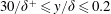 $30/\unicode[STIX]{x1D6FF}^{+}\leqslant y/\unicode[STIX]{x1D6FF}\leqslant 0.2$
then yields
$30/\unicode[STIX]{x1D6FF}^{+}\leqslant y/\unicode[STIX]{x1D6FF}\leqslant 0.2$
then yields
 $1/\unicode[STIX]{x1D705}_{\unicode[STIX]{x1D700}\unicode[STIX]{x1D703}}=2.18$
(viz.
$1/\unicode[STIX]{x1D705}_{\unicode[STIX]{x1D700}\unicode[STIX]{x1D703}}=2.18$
(viz.
 $\unicode[STIX]{x1D705}_{\unicode[STIX]{x1D700}\unicode[STIX]{x1D703}}=0.46$
) and
$\unicode[STIX]{x1D705}_{\unicode[STIX]{x1D700}\unicode[STIX]{x1D703}}=0.46$
) and
 $c_{\unicode[STIX]{x1D703}}=0.6$
and 1.5 for CHF and CHS, respectively (see figure 9
a,b). This finite Reynolds number effect comes from the effect of the mean pressure gradient, which is absent in a zero-pressure-gradient thermal boundary layer (Li et al.
Reference Li, Schlatter, Brandt and Henningson2009). When the finite Reynolds number effect disappears (
$c_{\unicode[STIX]{x1D703}}=0.6$
and 1.5 for CHF and CHS, respectively (see figure 9
a,b). This finite Reynolds number effect comes from the effect of the mean pressure gradient, which is absent in a zero-pressure-gradient thermal boundary layer (Li et al.
Reference Li, Schlatter, Brandt and Henningson2009). When the finite Reynolds number effect disappears (
 $h^{+}\geqslant 5000$
), equations (4.16) and (4.17) reduce to
$h^{+}\geqslant 5000$
), equations (4.16) and (4.17) reduce to
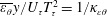 $\overline{\unicode[STIX]{x1D700}_{\unicode[STIX]{x1D703}}}y/U_{\unicode[STIX]{x1D70F}}T_{\unicode[STIX]{x1D70F}}^{2}=1/\unicode[STIX]{x1D705}_{\unicode[STIX]{x1D700}\unicode[STIX]{x1D703}}$
analogous to the classical scaling based on the scalar log law
$\overline{\unicode[STIX]{x1D700}_{\unicode[STIX]{x1D703}}}y/U_{\unicode[STIX]{x1D70F}}T_{\unicode[STIX]{x1D70F}}^{2}=1/\unicode[STIX]{x1D705}_{\unicode[STIX]{x1D700}\unicode[STIX]{x1D703}}$
analogous to the classical scaling based on the scalar log law
 $\overline{\unicode[STIX]{x1D700}_{\unicode[STIX]{x1D703}}}y/U_{\unicode[STIX]{x1D70F}}T_{\unicode[STIX]{x1D70F}}^{2}=1/\unicode[STIX]{x1D705}_{\unicode[STIX]{x1D703}}$
(see Abe & Antonia Reference Abe and Antonia2011).
$\overline{\unicode[STIX]{x1D700}_{\unicode[STIX]{x1D703}}}y/U_{\unicode[STIX]{x1D70F}}T_{\unicode[STIX]{x1D70F}}^{2}=1/\unicode[STIX]{x1D705}_{\unicode[STIX]{x1D703}}$
(see Abe & Antonia Reference Abe and Antonia2011).

Figure 9. Distributions of
 $P_{\unicode[STIX]{x1D703}}y/U_{\unicode[STIX]{x1D70F}}T_{\unicode[STIX]{x1D70F}}^{2}$
and
$P_{\unicode[STIX]{x1D703}}y/U_{\unicode[STIX]{x1D70F}}T_{\unicode[STIX]{x1D70F}}^{2}$
and
 $\overline{\unicode[STIX]{x1D700}_{\unicode[STIX]{x1D703}}}y/U_{\unicode[STIX]{x1D70F}}T_{\unicode[STIX]{x1D70F}}^{2}$
for
$\overline{\unicode[STIX]{x1D700}_{\unicode[STIX]{x1D703}}}y/U_{\unicode[STIX]{x1D70F}}T_{\unicode[STIX]{x1D70F}}^{2}$
for
 $Pr=0.71$
: (a)
$Pr=0.71$
: (a)
 $\overline{\unicode[STIX]{x1D700}_{\unicode[STIX]{x1D703}}}y/U_{\unicode[STIX]{x1D70F}}T_{\unicode[STIX]{x1D70F}}^{2}$
(CHF); (b)
$\overline{\unicode[STIX]{x1D700}_{\unicode[STIX]{x1D703}}}y/U_{\unicode[STIX]{x1D70F}}T_{\unicode[STIX]{x1D70F}}^{2}$
(CHF); (b)
 $\overline{\unicode[STIX]{x1D700}_{\unicode[STIX]{x1D703}}}y/U_{\unicode[STIX]{x1D70F}}T_{\unicode[STIX]{x1D70F}}^{2}$
(CHS); (c)
$\overline{\unicode[STIX]{x1D700}_{\unicode[STIX]{x1D703}}}y/U_{\unicode[STIX]{x1D70F}}T_{\unicode[STIX]{x1D70F}}^{2}$
(CHS); (c)
 $P_{\unicode[STIX]{x1D703}}y/U_{\unicode[STIX]{x1D70F}}T_{\unicode[STIX]{x1D70F}}^{2}$
(CHS); (d)
$P_{\unicode[STIX]{x1D703}}y/U_{\unicode[STIX]{x1D70F}}T_{\unicode[STIX]{x1D70F}}^{2}$
(CHS); (d)
 $\overline{\unicode[STIX]{x1D700}_{\unicode[STIX]{x1D703}}}y/U_{\unicode[STIX]{x1D70F}}T_{\unicode[STIX]{x1D70F}}^{2}$
(CHS). Note that (b) is replotted in (d) with different scales to highlight the overlap scaling of
$\overline{\unicode[STIX]{x1D700}_{\unicode[STIX]{x1D703}}}y/U_{\unicode[STIX]{x1D70F}}T_{\unicode[STIX]{x1D70F}}^{2}$
(CHS). Note that (b) is replotted in (d) with different scales to highlight the overlap scaling of
 $P_{\unicode[STIX]{x1D703}}$
and
$P_{\unicode[STIX]{x1D703}}$
and
 $\overline{\unicode[STIX]{x1D700}_{\unicode[STIX]{x1D703}}}$
.
$\overline{\unicode[STIX]{x1D700}_{\unicode[STIX]{x1D703}}}$
.
A comparison between the normalized
 $P_{\unicode[STIX]{x1D703}}$
and
$P_{\unicode[STIX]{x1D703}}$
and
 $\overline{\unicode[STIX]{x1D700}_{\unicode[STIX]{x1D703}}}$
(i.e.
$\overline{\unicode[STIX]{x1D700}_{\unicode[STIX]{x1D703}}}$
(i.e.
 $P_{\unicode[STIX]{x1D703}}y/U_{\unicode[STIX]{x1D70F}}T_{\unicode[STIX]{x1D70F}}^{2}$
and
$P_{\unicode[STIX]{x1D703}}y/U_{\unicode[STIX]{x1D70F}}T_{\unicode[STIX]{x1D70F}}^{2}$
and
 $\overline{\unicode[STIX]{x1D700}_{\unicode[STIX]{x1D703}}}y/U_{\unicode[STIX]{x1D70F}}T_{\unicode[STIX]{x1D70F}}^{2}$
) may provide further insight into the overlap scaling for large and small scales. Figure 9(c,d) indicates that the collapse is more convincing for
$\overline{\unicode[STIX]{x1D700}_{\unicode[STIX]{x1D703}}}y/U_{\unicode[STIX]{x1D70F}}T_{\unicode[STIX]{x1D70F}}^{2}$
) may provide further insight into the overlap scaling for large and small scales. Figure 9(c,d) indicates that the collapse is more convincing for
 $\overline{\unicode[STIX]{x1D700}_{\unicode[STIX]{x1D703}}}$
than for
$\overline{\unicode[STIX]{x1D700}_{\unicode[STIX]{x1D703}}}$
than for
 $P_{\unicode[STIX]{x1D703}}$
when
$P_{\unicode[STIX]{x1D703}}$
when
 $h^{+}$
is larger than 400. This is because the log-law conditions for mean temperature (i.e. constant
$h^{+}$
is larger than 400. This is because the log-law conditions for mean temperature (i.e. constant
 $\unicode[STIX]{x1D705}_{\unicode[STIX]{x1D703}}$
and
$\unicode[STIX]{x1D705}_{\unicode[STIX]{x1D703}}$
and
 $\overline{v\unicode[STIX]{x1D703}}$
) are required for the collapse of
$\overline{v\unicode[STIX]{x1D703}}$
) are required for the collapse of
 $P_{\unicode[STIX]{x1D703}}y/U_{\unicode[STIX]{x1D70F}}T_{\unicode[STIX]{x1D70F}}^{2}$
, while the overlap scaling of
$P_{\unicode[STIX]{x1D703}}y/U_{\unicode[STIX]{x1D70F}}T_{\unicode[STIX]{x1D70F}}^{2}$
, while the overlap scaling of
 $\overline{\unicode[STIX]{x1D700}_{\unicode[STIX]{x1D703}}}$
only requires the Reynolds number to be large enough. The same trend is also observed for the relationship between the turbulent kinetic energy production
$\overline{\unicode[STIX]{x1D700}_{\unicode[STIX]{x1D703}}}$
only requires the Reynolds number to be large enough. The same trend is also observed for the relationship between the turbulent kinetic energy production
 $P_{k}$
and the energy dissipation rate
$P_{k}$
and the energy dissipation rate
 $\overline{\unicode[STIX]{x1D700}}$
(see Abe & Antonia Reference Abe and Antonia2016). Note that
$\overline{\unicode[STIX]{x1D700}}$
(see Abe & Antonia Reference Abe and Antonia2016). Note that
 $P_{\unicode[STIX]{x1D703}}=\overline{\unicode[STIX]{x1D700}_{\unicode[STIX]{x1D703}}}$
does not hold strictly in the logarithmic and outer regions (see Pirozzoli et al.
Reference Pirozzoli, Bernardini and Orlandi2016) due to the presence of large-scale structures (see figure 3). This small departure from energy equilibrium however does not appear to affect the overlap scaling for
$P_{\unicode[STIX]{x1D703}}=\overline{\unicode[STIX]{x1D700}_{\unicode[STIX]{x1D703}}}$
does not hold strictly in the logarithmic and outer regions (see Pirozzoli et al.
Reference Pirozzoli, Bernardini and Orlandi2016) due to the presence of large-scale structures (see figure 3). This small departure from energy equilibrium however does not appear to affect the overlap scaling for
 $\overline{\unicode[STIX]{x1D6E9}}$
significantly since it is difficult to distinguish
$\overline{\unicode[STIX]{x1D6E9}}$
significantly since it is difficult to distinguish
 $\unicode[STIX]{x1D705}_{\unicode[STIX]{x1D703}}$
from
$\unicode[STIX]{x1D705}_{\unicode[STIX]{x1D703}}$
from
 $\unicode[STIX]{x1D705}_{\unicode[STIX]{x1D700}\unicode[STIX]{x1D703}}$
when the Reynolds number is sufficiently large (see figure 12). It would appear that the overlap region for the dissipation has indeed a higher rank than that for the mean field since the small scales (i.e. dissipation) are likely to ‘lose’ their dependence on the Reynolds number more rapidly than the large scales (i.e. the mean field).
$\unicode[STIX]{x1D705}_{\unicode[STIX]{x1D700}\unicode[STIX]{x1D703}}$
when the Reynolds number is sufficiently large (see figure 12). It would appear that the overlap region for the dissipation has indeed a higher rank than that for the mean field since the small scales (i.e. dissipation) are likely to ‘lose’ their dependence on the Reynolds number more rapidly than the large scales (i.e. the mean field).
Note that (4.16), (4.17) represent the outer scaling in a wider range of the
 $y$
location than expected, viz.
$y$
location than expected, viz.
 $$\begin{eqnarray}\overline{\unicode[STIX]{x1D700}_{\unicode[STIX]{x1D703}}}h/U_{\unicode[STIX]{x1D70F}}T_{\unicode[STIX]{x1D70F}}^{2}=2.18/(y/h)-c_{\unicode[STIX]{x1D703}}\end{eqnarray}$$
(see figure 10). In particular, there is excellent collapse of (4.18) for CHS up to the centreline (see figure 10
b), consistent with a smaller departure from the mean scalar log law (see figure 12
c where
 $1/\unicode[STIX]{x1D705}_{\unicode[STIX]{x1D703}}\equiv y^{+}(\text{d}\bar{\unicode[STIX]{x1D6E9}}^{+}/\text{d}y^{+})$
is plotted). This underlines the existence of a large overlap region for
$1/\unicode[STIX]{x1D705}_{\unicode[STIX]{x1D703}}\equiv y^{+}(\text{d}\bar{\unicode[STIX]{x1D6E9}}^{+}/\text{d}y^{+})$
is plotted). This underlines the existence of a large overlap region for
 $\overline{\unicode[STIX]{x1D700}_{\unicode[STIX]{x1D703}}}$
at
$\overline{\unicode[STIX]{x1D700}_{\unicode[STIX]{x1D703}}}$
at
 $Pr=0.71$
, as was observed for
$Pr=0.71$
, as was observed for
 $\overline{\unicode[STIX]{x1D6E9}}$
.
$\overline{\unicode[STIX]{x1D6E9}}$
.

Figure 10. Distributions of
 $\overline{\unicode[STIX]{x1D700}_{\unicode[STIX]{x1D703}}}h/U_{\unicode[STIX]{x1D70F}}T_{\unicode[STIX]{x1D70F}}^{2}$
for
$\overline{\unicode[STIX]{x1D700}_{\unicode[STIX]{x1D703}}}h/U_{\unicode[STIX]{x1D70F}}T_{\unicode[STIX]{x1D70F}}^{2}$
for
 $Pr=0.71$
with log–log coordinates: (a) CHF; (b) CHS.
$Pr=0.71$
with log–log coordinates: (a) CHF; (b) CHS.
4.4 Fractional contributions to
$\langle \overline{\unicode[STIX]{x1D700}_{\unicode[STIX]{x1D703}}}\rangle /U_{\unicode[STIX]{x1D70F}}T_{\unicode[STIX]{x1D70F}}^{2}$

It is of importance to clarify if the integral of
 $\overline{\unicode[STIX]{x1D700}_{\unicode[STIX]{x1D703}}}$
over the overlap region yields the logarithmic
$\overline{\unicode[STIX]{x1D700}_{\unicode[STIX]{x1D703}}}$
over the overlap region yields the logarithmic
 $h^{+}$
dependence of
$h^{+}$
dependence of
 $\langle \overline{\unicode[STIX]{x1D700}_{\unicode[STIX]{x1D703}}}\rangle /U_{\unicode[STIX]{x1D70F}}T_{\unicode[STIX]{x1D70F}}^{2}$
. In the present study, we follow the same approach as in Sreenivasan (Reference Sreenivasan, Deshpande, Prabhu, Sreenivasan and Viswanath1995) and Abe & Antonia (Reference Abe and Antonia2016) for
$\langle \overline{\unicode[STIX]{x1D700}_{\unicode[STIX]{x1D703}}}\rangle /U_{\unicode[STIX]{x1D70F}}T_{\unicode[STIX]{x1D70F}}^{2}$
. In the present study, we follow the same approach as in Sreenivasan (Reference Sreenivasan, Deshpande, Prabhu, Sreenivasan and Viswanath1995) and Abe & Antonia (Reference Abe and Antonia2016) for
 $\langle \overline{\unicode[STIX]{x1D700}}\rangle /U_{\unicode[STIX]{x1D70F}}^{3}$
, viz.
$\langle \overline{\unicode[STIX]{x1D700}}\rangle /U_{\unicode[STIX]{x1D70F}}^{3}$
, viz.
 $$\begin{eqnarray}\frac{\langle \overline{\unicode[STIX]{x1D700}_{\unicode[STIX]{x1D703}}}\rangle }{U_{\unicode[STIX]{x1D70F}}T_{\unicode[STIX]{x1D70F}}^{2}}=\underbrace{\int _{0}^{30}\overline{\unicode[STIX]{x1D700}_{\unicode[STIX]{x1D703}}}^{+}\text{d}y^{+}}_{C_{i}}+\underbrace{\int _{30\unicode[STIX]{x1D708}/U_{\unicode[STIX]{x1D70F}}}^{0.2h}\frac{\overline{\unicode[STIX]{x1D700}_{\unicode[STIX]{x1D703}}}}{U_{\unicode[STIX]{x1D70F}}T_{\unicode[STIX]{x1D70F}}^{2}}\,\text{d}y}_{C_{log}}+\underbrace{\int _{0.2}^{1}\frac{\overline{\unicode[STIX]{x1D700}_{\unicode[STIX]{x1D703}}}h}{U_{\unicode[STIX]{x1D70F}}T_{\unicode[STIX]{x1D70F}}^{2}}d\left(\frac{y}{h}\right)}_{C_{o}},\end{eqnarray}$$
where the limits for the second integral in (4.19) correspond to the extent of the overlap region of
 $\overline{\unicode[STIX]{x1D700}_{\unicode[STIX]{x1D703}}}$
for
$\overline{\unicode[STIX]{x1D700}_{\unicode[STIX]{x1D703}}}$
for
 $Pr=0.71$
(i.e. from
$Pr=0.71$
(i.e. from
 $y^{+}\simeq 30$
to
$y^{+}\simeq 30$
to
 $y/h=0.2$
). Values of
$y/h=0.2$
). Values of
 $C_{i}$
,
$C_{i}$
,
 $C_{log}$
and
$C_{log}$
and
 $C_{o}$
obtained from the present DNS data are shown in figure 11. Also included in this figure are the
$C_{o}$
obtained from the present DNS data are shown in figure 11. Also included in this figure are the
 $C_{log}$
and
$C_{log}$
and
 $C_{o}$
data of Pirozzoli et al. (Reference Pirozzoli, Bernardini and Orlandi2016) for
$C_{o}$
data of Pirozzoli et al. (Reference Pirozzoli, Bernardini and Orlandi2016) for
 $Pr=1$
since the outer layer similarity is convincing for
$Pr=1$
since the outer layer similarity is convincing for
 $\overline{\unicode[STIX]{x1D700}_{\unicode[STIX]{x1D703}}}h/U_{\unicode[STIX]{x1D70F}}T_{\unicode[STIX]{x1D70F}}^{2}$
(see figure 8
b). Clearly, there is a
$\overline{\unicode[STIX]{x1D700}_{\unicode[STIX]{x1D703}}}h/U_{\unicode[STIX]{x1D70F}}T_{\unicode[STIX]{x1D70F}}^{2}$
(see figure 8
b). Clearly, there is a
 $\ln (h^{+})$
dependence for
$\ln (h^{+})$
dependence for
 $C_{log}$
. This dependence is obtained by integrating (4.16) or (4.17), viz.
$C_{log}$
. This dependence is obtained by integrating (4.16) or (4.17), viz.
 $$\begin{eqnarray}C_{log}\simeq \displaystyle \int _{30\unicode[STIX]{x1D708}/U_{\unicode[STIX]{x1D70F}}}^{0.2h}\left(\frac{1}{\unicode[STIX]{x1D705}_{\unicode[STIX]{x1D700}\unicode[STIX]{x1D703}}y}-\frac{c_{\unicode[STIX]{x1D703}}}{h}\right)\,\text{d}y=2.18(\ln (h^{+})+\ln (0.2)-\ln (30))-c_{\unicode[STIX]{x1D703}}(0.2-30/h^{+}),\end{eqnarray}$$
in which the last term of (4.20), the finite Reynolds number effect, cannot be dismissed when
 $h^{+}$
is small. Given that
$h^{+}$
is small. Given that
 $C_{o}$
is essentially constant but the magnitude of
$C_{o}$
is essentially constant but the magnitude of
 $C_{i}$
increases slowly with
$C_{i}$
increases slowly with
 $h^{+}$
(figure 11), we integrate
$h^{+}$
(figure 11), we integrate
 $\overline{\unicode[STIX]{x1D700}_{\unicode[STIX]{x1D703}}}$
from
$\overline{\unicode[STIX]{x1D700}_{\unicode[STIX]{x1D703}}}$
from
 $y=0$
to
$y=0$
to
 $0.2h$
(viz.
$0.2h$
(viz.
 $C_{i}+C_{log}$
). The resulting integral is described adequately by
$C_{i}+C_{log}$
). The resulting integral is described adequately by
 $$\begin{eqnarray}C_{i}+C_{log}=\int _{0}^{0.2h}\frac{\langle \overline{\unicode[STIX]{x1D700}_{\unicode[STIX]{x1D703}}}\rangle }{U_{\unicode[STIX]{x1D70F}}T_{\unicode[STIX]{x1D70F}}^{2}}\,\text{d}y=2.18\ln (h^{+})-C_{2}\end{eqnarray}$$
for
 $h^{+}\geqslant 400$
with
$h^{+}\geqslant 400$
with
 $C_{2}=7.7$
and 8.2 for CHF and CHS, respectively. Note that the sum of (4.21) and
$C_{2}=7.7$
and 8.2 for CHF and CHS, respectively. Note that the sum of (4.21) and
 $C_{o}$
((2.5) and (2.1) for CHF and CHS, respectively) is identical to (4.6). This implies that the more appropriate expression for the logarithmic dependence of
$C_{o}$
((2.5) and (2.1) for CHF and CHS, respectively) is identical to (4.6). This implies that the more appropriate expression for the logarithmic dependence of
 $\langle \overline{\unicode[STIX]{x1D700}_{\unicode[STIX]{x1D703}}}\rangle /U_{\unicode[STIX]{x1D70F}}T_{\unicode[STIX]{x1D70F}}^{2}$
for the channel requires integration from
$\langle \overline{\unicode[STIX]{x1D700}_{\unicode[STIX]{x1D703}}}\rangle /U_{\unicode[STIX]{x1D70F}}T_{\unicode[STIX]{x1D70F}}^{2}$
for the channel requires integration from
 $y=0$
to
$y=0$
to
 $0.2h$
, viz. the contribution of
$0.2h$
, viz. the contribution of
 $C_{i}$
(
$C_{i}$
(
 $h^{+}$
) cannot be ignored. The present results highlight that the slope of 2.18 in (4.21) can be identified with
$h^{+}$
) cannot be ignored. The present results highlight that the slope of 2.18 in (4.21) can be identified with
 $1/\unicode[STIX]{x1D705}_{\unicode[STIX]{x1D700}\unicode[STIX]{x1D703}}$
as inferred from the overlap scaling of
$1/\unicode[STIX]{x1D705}_{\unicode[STIX]{x1D700}\unicode[STIX]{x1D703}}$
as inferred from the overlap scaling of
 $\overline{\unicode[STIX]{x1D700}_{\unicode[STIX]{x1D703}}}$
, and that
$\overline{\unicode[STIX]{x1D700}_{\unicode[STIX]{x1D703}}}$
, and that
 $1/\unicode[STIX]{x1D705}_{\unicode[STIX]{x1D700}\unicode[STIX]{x1D703}}$
is identical with the slope for the
$1/\unicode[STIX]{x1D705}_{\unicode[STIX]{x1D700}\unicode[STIX]{x1D703}}$
is identical with the slope for the
 $\ln (h^{+})$
dependence of the integrated mean scalar.
$\ln (h^{+})$
dependence of the integrated mean scalar.

Figure 11. Distributions of piecewise contributions to
 $\langle \overline{\unicode[STIX]{x1D700}_{\unicode[STIX]{x1D703}}}\rangle /U_{\unicode[STIX]{x1D70F}}T_{\unicode[STIX]{x1D70F}}^{2}$
for
$\langle \overline{\unicode[STIX]{x1D700}_{\unicode[STIX]{x1D703}}}\rangle /U_{\unicode[STIX]{x1D70F}}T_{\unicode[STIX]{x1D70F}}^{2}$
for
 $Pr=0.71$
as a function of
$Pr=0.71$
as a function of
 $h^{+}$
: (a) from
$h^{+}$
: (a) from
 $y^{+}$
 $=0$
to 30 (
$=0$
to 30 (
 $C_{i}$
); (b) from
$C_{i}$
); (b) from
 $y^{+}=30$
to
$y^{+}=30$
to
 $y/\unicode[STIX]{x1D6FF}=0.2$
(
$y/\unicode[STIX]{x1D6FF}=0.2$
(
 $C_{log}$
) and from
$C_{log}$
) and from
 $y/\unicode[STIX]{x1D6FF}=0$
to 0.2 (
$y/\unicode[STIX]{x1D6FF}=0$
to 0.2 (
 $C_{i}+C_{log}$
); (c) from
$C_{i}+C_{log}$
); (c) from
 $y/\unicode[STIX]{x1D6FF}=0.2$
to 1 (
$y/\unicode[STIX]{x1D6FF}=0.2$
to 1 (
 $C_{o}$
). ○, Present (CHF); ●, Present (CHS); ▪, Pirozzoli et al. (Reference Pirozzoli, Bernardini and Orlandi2016) for
$C_{o}$
). ○, Present (CHF); ●, Present (CHS); ▪, Pirozzoli et al. (Reference Pirozzoli, Bernardini and Orlandi2016) for
 $Pr=1$
.
$Pr=1$
.
When
 $h^{+}\rightarrow \infty$
, the overlap region should contribute exclusively to the
$h^{+}\rightarrow \infty$
, the overlap region should contribute exclusively to the
 $2.18\ln (h^{+})$
dependence of the integrated turbulent scalar energy dissipation rate. The present logarithmic
$2.18\ln (h^{+})$
dependence of the integrated turbulent scalar energy dissipation rate. The present logarithmic
 $h^{+}$
dependence of
$h^{+}$
dependence of
 $T_{b}^{+}$
and
$T_{b}^{+}$
and
 $T_{m}^{+}$
for CHS and CHF, respectively, is essentially linked to the excellent overlap region we observe for
$T_{m}^{+}$
for CHS and CHF, respectively, is essentially linked to the excellent overlap region we observe for
 $\overline{\unicode[STIX]{x1D700}_{\unicode[STIX]{x1D703}}}$
even at small
$\overline{\unicode[STIX]{x1D700}_{\unicode[STIX]{x1D703}}}$
even at small
 $h^{+}$
. Note that
$h^{+}$
. Note that
 $\unicode[STIX]{x1D705}_{\unicode[STIX]{x1D700}\unicode[STIX]{x1D703}}=0.46$
defined in (4.16), (4.17) is not identical with
$\unicode[STIX]{x1D705}_{\unicode[STIX]{x1D700}\unicode[STIX]{x1D703}}=0.46$
defined in (4.16), (4.17) is not identical with
 $\unicode[STIX]{x1D705}_{\unicode[STIX]{x1D703}}$
obtained from the scalar log law (4.1) for the Reynolds numbers examined (see figure 12). This is because, as for the mean velocity (see McKeon & Morrison Reference McKeon and Morrison2007, Smits, McKeon & Marusic Reference Smits, McKeon and Marusic2011), the constancy of
$\unicode[STIX]{x1D705}_{\unicode[STIX]{x1D703}}$
obtained from the scalar log law (4.1) for the Reynolds numbers examined (see figure 12). This is because, as for the mean velocity (see McKeon & Morrison Reference McKeon and Morrison2007, Smits, McKeon & Marusic Reference Smits, McKeon and Marusic2011), the constancy of
 $1/\unicode[STIX]{x1D705}_{\unicode[STIX]{x1D703}}\equiv y^{+}(\text{d}\bar{\unicode[STIX]{x1D6E9}}^{+}/\text{d}y^{+})$
is most likely to be established beyond
$1/\unicode[STIX]{x1D705}_{\unicode[STIX]{x1D703}}\equiv y^{+}(\text{d}\bar{\unicode[STIX]{x1D6E9}}^{+}/\text{d}y^{+})$
is most likely to be established beyond
 $h^{+}=5000$
(see figure 12
b) due to the non-negligible viscous effect (note that no collapse of the data is observed for
$h^{+}=5000$
(see figure 12
b) due to the non-negligible viscous effect (note that no collapse of the data is observed for
 $h^{+}=180$
due to the low Re effects). Figure 12 highlights the slow increase of
$h^{+}=180$
due to the low Re effects). Figure 12 highlights the slow increase of
 $\unicode[STIX]{x1D705}_{\unicode[STIX]{x1D703}}$
with increasing
$\unicode[STIX]{x1D705}_{\unicode[STIX]{x1D703}}$
with increasing
 $h^{+}$
, i.e.
$h^{+}$
, i.e.
 $\unicode[STIX]{x1D705}_{\unicode[STIX]{x1D703}}=0.40$
for
$\unicode[STIX]{x1D705}_{\unicode[STIX]{x1D703}}=0.40$
for
 $h^{+}=395$
(CHF) (Kawamura et al.
Reference Kawamura, Abe and Matsuo1999),
$h^{+}=395$
(CHF) (Kawamura et al.
Reference Kawamura, Abe and Matsuo1999),
 $\unicode[STIX]{x1D705}_{\unicode[STIX]{x1D703}}=0.43$
for
$\unicode[STIX]{x1D705}_{\unicode[STIX]{x1D703}}=0.43$
for
 $h^{+}=1020$
(CHF) (Abe et al.
Reference Abe, Kawamura and Matsuo2004a
) and
$h^{+}=1020$
(CHF) (Abe et al.
Reference Abe, Kawamura and Matsuo2004a
) and
 $\unicode[STIX]{x1D705}_{\unicode[STIX]{x1D703}}=0.46$
for
$\unicode[STIX]{x1D705}_{\unicode[STIX]{x1D703}}=0.46$
for
 $h^{+}=4088$
(CHS) (Pirozzoli et al.
Reference Pirozzoli, Bernardini and Orlandi2016). Pirozzoli et al. (Reference Pirozzoli, Bernardini and Orlandi2016) inferred
$h^{+}=4088$
(CHS) (Pirozzoli et al.
Reference Pirozzoli, Bernardini and Orlandi2016). Pirozzoli et al. (Reference Pirozzoli, Bernardini and Orlandi2016) inferred
 $\unicode[STIX]{x1D705}_{\unicode[STIX]{x1D703}}=0.46$
as the high Re asymptotic value on the basis of their datasets for the CHS case. Note that the departure from the scalar log law is smaller for CHS than for CHF due to the smaller magnitude of the mean scalar gradient, as discussed in § 4.1. Figure 12 also demonstrates that values of
$\unicode[STIX]{x1D705}_{\unicode[STIX]{x1D703}}=0.46$
as the high Re asymptotic value on the basis of their datasets for the CHS case. Note that the departure from the scalar log law is smaller for CHS than for CHF due to the smaller magnitude of the mean scalar gradient, as discussed in § 4.1. Figure 12 also demonstrates that values of
 $\unicode[STIX]{x1D705}$
and
$\unicode[STIX]{x1D705}$
and
 $\unicode[STIX]{x1D705}_{\unicode[STIX]{x1D703}}$
have most likely converged to different values (viz.
$\unicode[STIX]{x1D705}_{\unicode[STIX]{x1D703}}$
have most likely converged to different values (viz.
 $\unicode[STIX]{x1D705}=0.39$
and
$\unicode[STIX]{x1D705}=0.39$
and
 $\unicode[STIX]{x1D705}_{\unicode[STIX]{x1D703}}=0.46$
) at large Reynolds numbers, where the ratio
$\unicode[STIX]{x1D705}_{\unicode[STIX]{x1D703}}=0.46$
) at large Reynolds numbers, where the ratio
 $\unicode[STIX]{x1D705}/\unicode[STIX]{x1D705}_{\unicode[STIX]{x1D703}}\approx 0.85$
corresponds to the magnitude of
$\unicode[STIX]{x1D705}/\unicode[STIX]{x1D705}_{\unicode[STIX]{x1D703}}\approx 0.85$
corresponds to the magnitude of
 $\mathit{Pr}_{t}$
in the logarithmic region (see figure 2
b). Marusic et al. (Reference Marusic, Monty, Hultmark and Smits2013) reported
$\mathit{Pr}_{t}$
in the logarithmic region (see figure 2
b). Marusic et al. (Reference Marusic, Monty, Hultmark and Smits2013) reported
 $\unicode[STIX]{x1D705}=0.39$
in a laboratory boundary layer, pipe and atmospheric surface layer. Kader & Yaglom (Reference Kader and Yaglom1972) also analysed the experimental data in a channel, pipe and boundary layer for a wide range of the Reynolds number and concluded
$\unicode[STIX]{x1D705}=0.39$
in a laboratory boundary layer, pipe and atmospheric surface layer. Kader & Yaglom (Reference Kader and Yaglom1972) also analysed the experimental data in a channel, pipe and boundary layer for a wide range of the Reynolds number and concluded
 $\unicode[STIX]{x1D705}_{\unicode[STIX]{x1D703}}=0.47$
. Subramanian & Antonia (Reference Subramanian and Antonia1981) also reported
$\unicode[STIX]{x1D705}_{\unicode[STIX]{x1D703}}=0.47$
. Subramanian & Antonia (Reference Subramanian and Antonia1981) also reported
 $\unicode[STIX]{x1D705}_{\unicode[STIX]{x1D703}}=0.48\pm 0.02$
in a laboratory thermal boundary layer. The present value of
$\unicode[STIX]{x1D705}_{\unicode[STIX]{x1D703}}=0.48\pm 0.02$
in a laboratory thermal boundary layer. The present value of
 $\unicode[STIX]{x1D705}_{\unicode[STIX]{x1D700}\unicode[STIX]{x1D703}}=0.46$
may be reconcilable with the value of
$\unicode[STIX]{x1D705}_{\unicode[STIX]{x1D700}\unicode[STIX]{x1D703}}=0.46$
may be reconcilable with the value of
 $\unicode[STIX]{x1D705}_{\unicode[STIX]{x1D703}}$
(obtained at very large
$\unicode[STIX]{x1D705}_{\unicode[STIX]{x1D703}}$
(obtained at very large
 $h^{+}$
) if one recognizes that the outer layer similarity of
$h^{+}$
) if one recognizes that the outer layer similarity of
 $\overline{\unicode[STIX]{x1D700}_{\unicode[STIX]{x1D703}}}$
is established at a much smaller
$\overline{\unicode[STIX]{x1D700}_{\unicode[STIX]{x1D703}}}$
is established at a much smaller
 $h^{+}$
than for
$h^{+}$
than for
 $\overline{\unicode[STIX]{x1D6E9}}^{+}$
. Indeed, this appears to be adequately supported by the available DNS data (see figure 8).
$\overline{\unicode[STIX]{x1D6E9}}^{+}$
. Indeed, this appears to be adequately supported by the available DNS data (see figure 8).

Figure 12. Distributions of
 $y^{+}(\text{d}\overline{U}^{+}/\text{d}y^{+})$
and
$y^{+}(\text{d}\overline{U}^{+}/\text{d}y^{+})$
and
 $y^{+}(\text{d}\overline{\unicode[STIX]{x1D6E9}}^{+}/\text{d}y^{+})$
for
$y^{+}(\text{d}\overline{\unicode[STIX]{x1D6E9}}^{+}/\text{d}y^{+})$
for
 $Pr=0.71$
: (a)
$Pr=0.71$
: (a)
 $y^{+}(\text{d}\overline{U}^{+}/\text{d}y^{+})$
; (b)
$y^{+}(\text{d}\overline{U}^{+}/\text{d}y^{+})$
; (b)
 $y^{+}(\text{d}\overline{\unicode[STIX]{x1D6E9}}^{+}/\text{d}y^{+})$
(CHF); (c)
$y^{+}(\text{d}\overline{\unicode[STIX]{x1D6E9}}^{+}/\text{d}y^{+})$
(CHF); (c)
 $y^{+}(\text{d}\overline{\unicode[STIX]{x1D6E9}}^{+}/\text{d}y^{+})$
(CHS).
$y^{+}(\text{d}\overline{\unicode[STIX]{x1D6E9}}^{+}/\text{d}y^{+})$
(CHS).
5 Conclusions
The integration of mean and turbulent scalar dissipation rates across half the channel (which is equivalent to performing a global energy balance) has been carried out using the present DNS datasets (up to
 $h^{+}=1000$
) in a fully developed turbulent channel flow with passive scalar transport for
$h^{+}=1000$
) in a fully developed turbulent channel flow with passive scalar transport for
 $Pr=0.71$
. The results are compared with those obtained from existing DNS datasets up to
$Pr=0.71$
. The results are compared with those obtained from existing DNS datasets up to
 $h^{+}=4000$
. Two isothermal conditions (i.e. CHS and CHF) have been examined. After clarifying the difference between these conditions, unambiguous relations for the dependence of
$h^{+}=4000$
. Two isothermal conditions (i.e. CHS and CHF) have been examined. After clarifying the difference between these conditions, unambiguous relations for the dependence of
 $T_{b}^{+}$
(CHS) and
$T_{b}^{+}$
(CHS) and
 $T_{m}^{+}$
(CHF) on
$T_{m}^{+}$
(CHF) on
 $h^{+}$
have been obtained based on the energy balances for both the mean and turbulent scalar variance. The scaling behaviour of the turbulent scalar dissipation rate has also been carefully examined in order to confirm the logarithmic dependence of
$h^{+}$
have been obtained based on the energy balances for both the mean and turbulent scalar variance. The scaling behaviour of the turbulent scalar dissipation rate has also been carefully examined in order to confirm the logarithmic dependence of
 $T_{b}^{+}$
and
$T_{b}^{+}$
and
 $T_{m}^{+}$
on
$T_{m}^{+}$
on
 $h^{+}$
. The main conclusions are as follows.
$h^{+}$
. The main conclusions are as follows.
After normalizing by
 $U_{\unicode[STIX]{x1D70F}}T_{\unicode[STIX]{x1D70F}}^{2}$
, the scalar dissipation function, or sum of the integrals of the mean and turbulent scalar dissipation rates, is equal to
$U_{\unicode[STIX]{x1D70F}}T_{\unicode[STIX]{x1D70F}}^{2}$
, the scalar dissipation function, or sum of the integrals of the mean and turbulent scalar dissipation rates, is equal to
 $T_{b}^{+}$
and
$T_{b}^{+}$
and
 $T_{m}^{+}$
(i.e. equations (2.12)–(2.13)) for CHS and CHF, respectively. The logarithmic
$T_{m}^{+}$
(i.e. equations (2.12)–(2.13)) for CHS and CHF, respectively. The logarithmic
 $h^{+}$
dependence is established quite well (i.e. with significant confidence and minimal ambiguity) for the integrated mean scalar provided
$h^{+}$
dependence is established quite well (i.e. with significant confidence and minimal ambiguity) for the integrated mean scalar provided
 $h^{+}\geqslant 400$
where the integral of the mean scalar dissipation rate associated with the mean scalar gradient, i.e.
$h^{+}\geqslant 400$
where the integral of the mean scalar dissipation rate associated with the mean scalar gradient, i.e.
 $\langle a(\text{d}\overline{\unicode[STIX]{x1D6E9}}/\text{d}y)^{2}\rangle$
, normalized by
$\langle a(\text{d}\overline{\unicode[STIX]{x1D6E9}}/\text{d}y)^{2}\rangle$
, normalized by
 $U_{\unicode[STIX]{x1D70F}}T_{\unicode[STIX]{x1D70F}}^{2}$
, is essentially constant, whereas
$U_{\unicode[STIX]{x1D70F}}T_{\unicode[STIX]{x1D70F}}^{2}$
, is essentially constant, whereas
 $\langle \overline{\unicode[STIX]{x1D700}_{\unicode[STIX]{x1D703}}}\rangle /U_{\unicode[STIX]{x1D70F}}T_{\unicode[STIX]{x1D70F}}^{2}$
increases logarithmically with increasing
$\langle \overline{\unicode[STIX]{x1D700}_{\unicode[STIX]{x1D703}}}\rangle /U_{\unicode[STIX]{x1D70F}}T_{\unicode[STIX]{x1D70F}}^{2}$
increases logarithmically with increasing
 $h^{+}$
. Viscosity affects
$h^{+}$
. Viscosity affects
 $\langle a(\text{d}\overline{\unicode[STIX]{x1D6E9}}/\text{d}y)^{2}\rangle /U_{\unicode[STIX]{x1D70F}}T_{\unicode[STIX]{x1D70F}}^{2}$
significantly for
$\langle a(\text{d}\overline{\unicode[STIX]{x1D6E9}}/\text{d}y)^{2}\rangle /U_{\unicode[STIX]{x1D70F}}T_{\unicode[STIX]{x1D70F}}^{2}$
significantly for
 $h^{+}<400$
. The logarithmic
$h^{+}<400$
. The logarithmic
 $h^{+}$
dependence of
$h^{+}$
dependence of
 $\langle \overline{\unicode[STIX]{x1D700}_{\unicode[STIX]{x1D703}}}\rangle /U_{\unicode[STIX]{x1D70F}}T_{\unicode[STIX]{x1D70F}}^{2}$
is hence linked to that of
$\langle \overline{\unicode[STIX]{x1D700}_{\unicode[STIX]{x1D703}}}\rangle /U_{\unicode[STIX]{x1D70F}}T_{\unicode[STIX]{x1D70F}}^{2}$
is hence linked to that of
 $T_{b}^{+}$
or
$T_{b}^{+}$
or
 $T_{m}^{+}$
. The resulting relation for the heat transfer coefficient (4.7) is supported convincingly by the DNS data for CHF in the range
$T_{m}^{+}$
. The resulting relation for the heat transfer coefficient (4.7) is supported convincingly by the DNS data for CHF in the range
 $h^{+}\geqslant 200$
. The lower
$h^{+}\geqslant 200$
. The lower
 $h^{+}$
bound of (4.7) is about by a factor of 3 smaller than that of (1.10) derived by Kader & Yaglom (Reference Kader and Yaglom1972) from the log law in a pipe flow.
$h^{+}$
bound of (4.7) is about by a factor of 3 smaller than that of (1.10) derived by Kader & Yaglom (Reference Kader and Yaglom1972) from the log law in a pipe flow.
Support for the logarithmic
 $h^{+}$
dependence of
$h^{+}$
dependence of
 $\langle \overline{\unicode[STIX]{x1D700}_{\unicode[STIX]{x1D703}}}\rangle /U_{\unicode[STIX]{x1D70F}}T_{\unicode[STIX]{x1D70F}}^{2}$
is provided by the scaling behaviour of the mean turbulent scalar dissipation rate. The inner layer scaling, i.e.
$\langle \overline{\unicode[STIX]{x1D700}_{\unicode[STIX]{x1D703}}}\rangle /U_{\unicode[STIX]{x1D70F}}T_{\unicode[STIX]{x1D70F}}^{2}$
is provided by the scaling behaviour of the mean turbulent scalar dissipation rate. The inner layer scaling, i.e.
 $\overline{\unicode[STIX]{x1D700}_{\unicode[STIX]{x1D703}}}\unicode[STIX]{x1D708}/U_{\unicode[STIX]{x1D70F}}^{2}T_{\unicode[STIX]{x1D70F}}^{2}=f(y^{+},Pr)$
, does not hold for
$\overline{\unicode[STIX]{x1D700}_{\unicode[STIX]{x1D703}}}\unicode[STIX]{x1D708}/U_{\unicode[STIX]{x1D70F}}^{2}T_{\unicode[STIX]{x1D70F}}^{2}=f(y^{+},Pr)$
, does not hold for
 $y^{+}\leqslant 30$
. On the other hand,
$y^{+}\leqslant 30$
. On the other hand,
 $\overline{\unicode[STIX]{x1D700}_{\unicode[STIX]{x1D703}}}$
collapses almost perfectly with
$\overline{\unicode[STIX]{x1D700}_{\unicode[STIX]{x1D703}}}$
collapses almost perfectly with
 $U_{\unicode[STIX]{x1D70F}}T_{\unicode[STIX]{x1D70F}}^{2}$
and
$U_{\unicode[STIX]{x1D70F}}T_{\unicode[STIX]{x1D70F}}^{2}$
and
 $h$
in the region
$h$
in the region
 $30/h^{+}<y/h<1$
. Unlike the mean scalar, the turbulent scalar dissipation rate is not affected significantly by viscosity for
$30/h^{+}<y/h<1$
. Unlike the mean scalar, the turbulent scalar dissipation rate is not affected significantly by viscosity for
 $y^{+}>30$
. Whereas the classical overlap argument based on
$y^{+}>30$
. Whereas the classical overlap argument based on
 $\overline{\unicode[STIX]{x1D6E9}}$
strictly holds only at large
$\overline{\unicode[STIX]{x1D6E9}}$
strictly holds only at large
 $h^{+}$
(Monin & Yaglom Reference Monin and Yaglom1971; Kader Reference Kader1981), the overlap region for
$h^{+}$
(Monin & Yaglom Reference Monin and Yaglom1971; Kader Reference Kader1981), the overlap region for
 $\overline{\unicode[STIX]{x1D700}_{\unicode[STIX]{x1D703}}}$
is established at small
$\overline{\unicode[STIX]{x1D700}_{\unicode[STIX]{x1D703}}}$
is established at small
 $h^{+}$
(
$h^{+}$
(
 ${\approx}400$
) independently of the existence of a scalar log law. It does however require the Reynolds number to be large enough (
${\approx}400$
) independently of the existence of a scalar log law. It does however require the Reynolds number to be large enough (
 $h^{+}\approx 400$
) to allow an overlap region where the relevant length scale is
$h^{+}\approx 400$
) to allow an overlap region where the relevant length scale is
 $y$
. In this region (
$y$
. In this region (
 $30/h^{+}\leqslant y/h\leqslant 0.2$
),
$30/h^{+}\leqslant y/h\leqslant 0.2$
),
 $\overline{\unicode[STIX]{x1D700}_{\unicode[STIX]{x1D703}}}y/U_{\unicode[STIX]{x1D70F}}T_{\unicode[STIX]{x1D70F}}^{2}$
approaches a constant (
$\overline{\unicode[STIX]{x1D700}_{\unicode[STIX]{x1D703}}}y/U_{\unicode[STIX]{x1D70F}}T_{\unicode[STIX]{x1D70F}}^{2}$
approaches a constant (
 $\unicode[STIX]{x1D705}_{\unicode[STIX]{x1D700}\unicode[STIX]{x1D703}}^{-1}=2.18$
), allowing for a finite Reynolds number correction, equations (4.16), (4.17), for
$\unicode[STIX]{x1D705}_{\unicode[STIX]{x1D700}\unicode[STIX]{x1D703}}^{-1}=2.18$
), allowing for a finite Reynolds number correction, equations (4.16), (4.17), for
 $h^{+}\geqslant 400$
. When
$h^{+}\geqslant 400$
. When
 $h^{+}$
is sufficiently large (
$h^{+}$
is sufficiently large (
 ${\geqslant}5000$
) (see figure 12
b) for the scalar log law to be established over a region where
${\geqslant}5000$
) (see figure 12
b) for the scalar log law to be established over a region where
 $P_{\unicode[STIX]{x1D703}}\simeq \overline{\unicode[STIX]{x1D700}_{\unicode[STIX]{x1D703}}}$
and
$P_{\unicode[STIX]{x1D703}}\simeq \overline{\unicode[STIX]{x1D700}_{\unicode[STIX]{x1D703}}}$
and
 $-\overline{v\unicode[STIX]{x1D703}}\simeq$
constant, the von Kármán constant for the mean scalar
$-\overline{v\unicode[STIX]{x1D703}}\simeq$
constant, the von Kármán constant for the mean scalar
 $\unicode[STIX]{x1D705}_{\unicode[STIX]{x1D703}}=0.46$
can be identified with
$\unicode[STIX]{x1D705}_{\unicode[STIX]{x1D703}}=0.46$
can be identified with
 $\unicode[STIX]{x1D705}_{\unicode[STIX]{x1D700}\unicode[STIX]{x1D703}}$
; the ratio
$\unicode[STIX]{x1D705}_{\unicode[STIX]{x1D700}\unicode[STIX]{x1D703}}$
; the ratio
 $\unicode[STIX]{x1D705}/\unicode[STIX]{x1D705}_{\unicode[STIX]{x1D703}}\approx 0.85$
corresponds to the value of
$\unicode[STIX]{x1D705}/\unicode[STIX]{x1D705}_{\unicode[STIX]{x1D703}}\approx 0.85$
corresponds to the value of
 $\mathit{Pr}_{t}$
in the overlap region. The enhanced scalar transport by vortical motions is also responsible for the decrease of
$\mathit{Pr}_{t}$
in the overlap region. The enhanced scalar transport by vortical motions is also responsible for the decrease of
 $\mathit{Pr}_{t}$
towards the centreline. The present logarithmic
$\mathit{Pr}_{t}$
towards the centreline. The present logarithmic
 $h^{+}$
dependence of
$h^{+}$
dependence of
 $T_{b}^{+}$
and
$T_{b}^{+}$
and
 $T_{m}^{+}$
follows from the overlap argument based entirely on the behaviour of
$T_{m}^{+}$
follows from the overlap argument based entirely on the behaviour of
 $\overline{\unicode[STIX]{x1D700}_{\unicode[STIX]{x1D703}}}$
in the inner and outer regions. We stress that the outer layer similarity of
$\overline{\unicode[STIX]{x1D700}_{\unicode[STIX]{x1D703}}}$
in the inner and outer regions. We stress that the outer layer similarity of
 $\overline{\unicode[STIX]{x1D700}_{\unicode[STIX]{x1D703}}}$
is more convincing than that of
$\overline{\unicode[STIX]{x1D700}_{\unicode[STIX]{x1D703}}}$
is more convincing than that of
 $\overline{\unicode[STIX]{x1D6E9}}$
and is established at a smaller value of
$\overline{\unicode[STIX]{x1D6E9}}$
and is established at a smaller value of
 $h^{+}$
(see figure 8). This is the reason why the present
$h^{+}$
(see figure 8). This is the reason why the present
 $T_{b}^{+}$
and
$T_{b}^{+}$
and
 $T_{m}^{+}$
relations (4.5), (4.4) are validated over a wide range of
$T_{m}^{+}$
relations (4.5), (4.4) are validated over a wide range of
 $h^{+}$
and are established at a lower Reynolds number than the mean temperature log law.
$h^{+}$
and are established at a lower Reynolds number than the mean temperature log law.
The establishment of the slopes for the logarithmic skin friction law (i.e. 2.54) (see Abe & Antonia Reference Abe and Antonia2016) and heat transfer law (i.e. 2.18) at small
 $h^{+}$
is an important outcome resulting from the present approach, viz. the use of the global energy budget, since these slopes are intrinsically associated with the ‘asymptotic’ values of the log-law slopes even though the mean velocity and mean temperature have yet to reach their asymptotic state.
$h^{+}$
is an important outcome resulting from the present approach, viz. the use of the global energy budget, since these slopes are intrinsically associated with the ‘asymptotic’ values of the log-law slopes even though the mean velocity and mean temperature have yet to reach their asymptotic state.
Acknowledgements
Computations performed on the JAXA (Japan Aerospace Exploration Agency) Supercomputer System are gratefully acknowledged. H.A. is grateful to Professor H. Kawamura and Dr Y. Matsuo for earlier collaborations.


