


1. INTRODUCTION
Building construction projects are mostly linear processes, but can iterate when faults occur. These iterations add time and cost to the construction process, especially if the iteration was not anticipated (Mitropoulos & Howell, Reference Mitropoulos and Howell2002). There are several reasons for unanticipated iteration in a construction project, including a poor brief, political considerations, or an insufficient budget. The disruption to the project frequently occurs later on in the execution of the project (Chester & Hendrickson, Reference Chester and Hendrickson2005). In these events, it would be beneficial to be provided with early warning that a type of problem was anticipated. If some signal could be observed early in the process, the project manager could be made aware of the potential problem and take mitigating action.
This research seeks to exploit Bayesian methods to interpret a single signal based on the temporal progress of a project to generate diagnostic predictions of potential problems. The Bayesian method will produce a set of probabilities that certain problems exist. It will then be for the project manager to interpret these in the broader context of the project execution as to what action would be appropriate. This is a significant development on previous work, such as that of Weidl, Madsen, and Israelson (Reference Weidl, Madsen and Israelson2005) and Lee, Park, and Shin (Reference Lee, Park and Shin2009), where multiple signals are used, which are often subjective. The diagnosis method presented in this article aids the project manager in focusing on a small number of potential problems, but it still encourages project managers to apply their own judgment.
The remainder of this article will first present background to this research. This will then be synthesized into a Markov-like process model for the construction domain. This process model will then be presented with certain scenarios and the results will be analyzed. Finally, there will be a discussion regarding the model in the domain context. The article will then conclude with comments on the general approach.
2. BACKGROUND
Process planning and scheduling are mature topics. These are essential tools that support the ability to deliver project outcomes in a timely and ordered manner. “Modern” tools, such as PERT and critical planning, have been well studied and adopted (Kelley & Walker, Reference Kelley and Walker1959; Williams, Reference Williams1995). Although they provide the means for estimating the duration of a project and identifying that a project is off-track, they do not provide guidance as to what is causing the difficulty. As increasingly complex projects are planned with greater sources of uncertainty, these original methods need to be extended to be able to handle a more stochastic view of planning and scheduling.
The construction industry follows a (mostly) linear process. This process starts with the project inception and definition and is expected to terminate with the completion of the building. The process can terminate in other ways, but these represent project failures, because the project has come to a conclusion other than completing the building. Within this process, there are also gateways (Soibelman et al., Reference Soibelman, Liu, Kirby, East, Caldas and Lin2003). These gateways ensure that the project has reached sufficient maturity and quality that it may proceed to the next phase. In the event that a gateway blocks the project, two outcomes are possible: either the process must return to the start of the phase or the project is terminated (i.e., it fails).
For the purposes of this research, the Royal Institute of British Architects (RIBA) construction process is adopted (RIBA, 2007). Figure 1 contains the earliest part of that process, represented as a flowchart. This flowchart starts with the project inception and terminates at the granting of building permission. The process continues with the construction of the building. For the purposes of this article, it is sufficient to only consider the earliest phases, and the study will focus on the RIBA process up to and including the first gateway review (GR1).
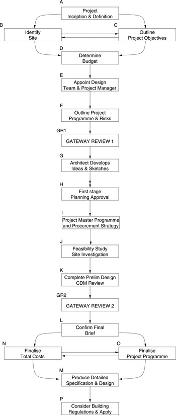
Fig. 1. Overview of the full early phases of the Royal Institute of British Architects process.
This flowchart can be thought of as a Markov chain, as illustrated in Figure 2 (Wu & Shieh, Reference Wu and Shieh2006; Taha, Reference Taha2007). Each element of the flowchart can be represented by a node. From each node, there are a number of nodes the process could progress to, which are represented by the directed arcs exiting the node. For example, from the identify site node, the process could move on to any of outline objectives, determine budget, or project definition. This does assume that projects only perform one task at a time, but for the purpose of this research this is not critical. When simulating the design process, the node that the process moves to is determined stochastically. In other words, each arc has a predetermined probability of being followed. Based on these probabilities, an arc is selected at random thereby moving the process on to the next step. For the simulation model, these probabilities were estimated through a combination of literature and discussions with domain experts.

Fig. 2. Detailed view of the quasi-Markov chain implementation of the Royal Institute of British Architects process for this study.
2.1. Construction design process
The construction design process is a variant of generic product development, as described by, for example, Pahl and Beitz (Reference Pahl and Beitz1996) and Cross (Reference Cross2000). The fundamental aspects of this process are mostly linear, but divided into major sections (i.e., phases) that are delimited by stage gates (Soibelman et al., Reference Soibelman, Liu, Kirby, East, Caldas and Lin2003). These stage gates provide the opportunity to review the progress of the project and determine if it should go ahead, require further work within the current stage, or be terminated. This ensures that “weak” designs are not taken through to further downstream phases (thereby wasting resource or risking failure; Von Stamm, Reference Von Stamm2008).
The construction industry ranges from building construction through to highway laying. This article will focus on building construction, due to its generality: individual building professionals (e.g., architects, builders) tend to specialize in certain types of buildings due to the level of specialist knowledge that is required. There is common ground, however, across all these specialist domains. First, the design stage is common to all domains. The client proposes an idea for a building project and it is then up to the architect to transform this idea into a practical building solution. To achieve this successfully, the design must satisfy the client's requirement for both the functionality and aesthetics of the building. Second, the financial considerations of a building project are common. There is typically a fixed overall budget with little leeway vis-à-vis the total cost. The client will have expectations of what can be achieved for her or his budget and it is the architect's responsibility to provide solutions that can maximize what can be achieved for that budget. Third, the consideration of and adherence to legal issues is common. There are a significant number of legal regulations that buildings must follow. Although there will be different specialized legislation for different types of building projects, the overall process of following legislation remains common.
In the United Kingdom, the building process is governed by a set of rules detailed by RIBA. These rules divide the construction process into several stages:
1. preparation,
2. design,
3. preconstruction,
4. construction, and
5. use.
Each main stage is then broken down into smaller work stages. This work will focus on the first two of the main RIBA stages: preparation and design. These stages occur before significant resources have been invested into the project, and therefore it is during these stages when it is easiest (i.e., most cost effective) to change the design. The reasons for changing design could include misinterpretation, a change in budget, or a change of opinion.
Clough et al. (Reference Clough, Sears and Sears2000) note that the planning and definition stages of the project must define the requirements and (budgetary) constraints. The project definition must include “establishing broad project characteristics such as location, performance criteria, layout, equipment, services and other owner requirements needed to establish the general aspect of the project.” The design phase involves completing the architectural and engineering design of the entire project. This results in the production of the final working drawings and the specifications of the total construction program.
Ritz (Reference Ritz1994) states that the most critical stages of the preconstruction phase are the planning for construction execution and resource (i.e., time, money, equipment) usage. In projects where these aspects are neglected, there is a greater risk of project of failure at a later stage due to overruns of time and/or money.
Any significant construction project will have a number of independent parties involved. A key factor in the success of a construction project lies, therefore, within the communication between these parties (Chan et al., Reference Chan, Chan, Chiang, Tang, Chan and Ho2004). In particular, it is the quality of the communication at certain key points within the process that has a significant impact on the outcome of the project (Emmitt & Gorse, Reference Emmitt and Gorse2003). These key points are characterized by where a decision has to be made that would be extremely difficult to change once the decision has been implemented. Lack of communication may result in changes having to be made, and these changes can result in negative consequences. An example of poor communication could occur when deciding the shape and floor plan of a building: if the appropriate parties are not made aware of a bad decision, there are several significant downstream design aspects that could be affected with potentially damaging results.
The challenges listed above give rise to the potentially difficult scenarios a construction process can find itself in. These are detailed in Table 1.
Table 1. Problematic construction process scenarios

2.2. Uncertainty within construction
Construction projects frequently overrun, either in terms of time or financial resources. Given that the budgets are set before any (physical) work is done, this is perhaps not surprising. The early phases of the construction process essentially serve to formulate an executive plan of work. The resources required for the various tasks involved are based on estimates and assumptions of how well the work will progress. These estimates and assumptions form the first source of uncertainty.
The construction process is complex, and contains a number of actors (e.g., client, architect, builder, and planners). Although the interaction among these actors is defined in terms of when they should occur and how they should proceed, there is no guarantee that this will happen. Moreover, the quality of the interaction is determined by the abilities of each actor. Ineffective or poor actions taken by certain actors will generate unacceptable work or fail to meet predetermined deadlines. Unacceptable work will require rework, which in turn will cause delays (Mitropoulos & Howell, Reference Mitropoulos and Howell2002). These events occur seemingly randomly (although will be biased by the capabilities of the various actors), and hence represent the second source of uncertainty.
Finally, the construction process occurs outdoors. In this context, there are external events beyond the control of any of the actors within the construction process, such as extreme weather. This introduces the third and final source of uncertainty.
2.3. Project monitoring and risk management
There have been a number of attempts to model the construction process stochastically (as well as other processes, such as the software engineering process). There are two levels at which these models operate: the first is to simply simulate the process under certain conditions; the second is to diagnose the process based on certain observations. Both these approaches require an understanding of the sources of uncertainty and the structural relationships between the various tasks within the processes.
The first level of model focused on process simulation. Chapman (Reference Chapman1990) was one of the earliest to use the term risk engineering. This was applied to an offshore pipeline laying project consisting of five key tasks. The duration of each of these tasks is represented by a probability distribution along with the number of days that are workable each month of the year. The simulation model's output provides a clearer picture of the overall project risks given these conditions, which are, in turn, used to decide when and how best to proceed with the pipe-laying project. Fenton et al. (Reference Fenton, Krause and Neil2002) and Khodakarami et al. (Reference Khodakarami, Fenton and Neil2007) use Bayesian belief networks (BBNs) to model and simulate the software engineering process. In Fenton et al. (Reference Fenton, Krause and Neil2002), the simulation is used to estimate the number of software defects in complex software packages based on a number of project characteristics, such as level of project complexity and development process maturity. This simulation provides a distribution of the possible number of faults, and enables a project manager to compare various options for shaping the project. A similar simulation approach is taken in Khodakarami et al. (Reference Khodakarami, Fenton and Neil2007) to estimate the total software engineering process duration. Neil et al. (Reference Neil, Fenton and Tailor2005) use a Bayesian network to assess financial institutions' exposure to rare but significant risk based on simulations using some basic stochastic estimates on frequency of extreme events and severity of extreme events. Moving to the construction process domain, Anderson et al. (Reference Anderson, Mukherjee and Onder2009) simulate the construction process using as a planning and constraint satisfaction problem with stochastic task durations. This supports different scenarios being simulated by modifying the probabilities that certain events will occur, which in turn will have an impact on the duration of the project. This enables a project manager to better plan for contingencies. Nasir et al. (Reference Nasir, McCabe and Hartono2003) identify a set of schedule-affected risks and construct a BBN based on these risks. Assuming a project manager knows which risks are occurring; this can then be used in a Monte Carlo simulation to compute a revised project duration estimate. Kim and Reinschmidt (Reference Kim and Reinschmidt2009) adopt a similar approach, but use the percentage of project completion as an input to estimate the overall completion date. Finally, Cho and Eppinger (Reference Cho and Eppinger2005) use design structure matrices, an approach similar to Markov chains, to rearrange task orders to minimize the effect of iterations within the design process.
The second level of modeling seeks to diagnose a given process. McCabe et al. (Reference McCabe, AbouRizk and Goebel1998) describe an early attempt to use BBNs to diagnose a construction process by observing queue lengths for various construction services related to a project. In the software engineering domain, Fan and Yu (Reference Fan and Yu2004) use a BBN to infer the risk level for a given software project based on observations such as developer experience and time pressures. The result is used to determine if the project has an appropriate level of resouces allocated to it. Lee et al. (Reference Lee, Park and Shin2009) use a BBN to identify potential risk sources in a project based on the observed risk level of a set of 26 identified risk categories. Through partial observation (or estimation) of some of these risks within a project, it is possible to identify the driving risk factors in the project and, therefore, support the management of these risks by the project manager. Weidl et al. (Reference Weidl, Madsen and Israelson2005) construct a BBN to monitor a large continuous process. Again, this is based on observed variables that are fed into the BBN. The BBN then presents a ranked set of potential root causes for any potential problems by identifying the variables that are driving the system into a problem state. Dissanayake and Robinson Fayek (Reference Dissanayake and Robinson Fayek2008) provide a project diagnosis tool based on fuzzy logic that is capable of identifying what might be affecting a particular task within a larger construction project.
2.4. Conclusion
The general construction process can be reasonably modeled as a Markov chain, with probabilistic transitions from one activity to the next. Although for any specific project there will have been deterministic reasons for moving from one activity to the next, this is not important when considering a large set of projects that will appear to move the process at random. Moreover, given that the exact nature of uncertainty in a current project is unknown, the best estimate that can be made for the transition probabilities at the outset are given by prior probabilities. In other words, when thinking about the future possible directions for a project that is about to start, a stochastic approach is suitable. As more information is gathered, this can be used to refine the understanding of the nature of project being executed.
3. PROCESS MODELING METHODOLOGY
The process modeling methodology is based on a Markov chain (Eckert et al., Reference Eckert, Clarkson and Zanker2004; Flanagan et al., Reference Flanagan, Eckert and Clarkson2007; Pandelis, Reference Pandelis2010). A Markov chain consists of a set of nodes linked by directed arcs. The temporal domain is modeled discretely, that is, one action happens per discrete time step. The nodes represent activities and the arcs represent the possible subsequent nodes the process could move to in the next time step, potentially including a “loop-back” arc, which models the process remaining in the same state at the next time step.
One aim of this work has been to make this approach broadly applicable within the construction industry. In order to achieve this, the key generic process stages in the early construction process were identified, based upon the RIBA framework. These stages are represented as nodes in the Markov chain (see Figure 1). The nodes are the following:
A. Project inception and definition: the “official” start of the project; formulating the core ideas of the project
B. Identify site: selection of the project location
C. Outline project objectives: specification of the fundamental design ideas
D. Determine budget: identify the total funding for the project
E. Appoint design team and project manager: identify the team of individuals who will execute the construction project
F. Outline project program and risks: define the various stages within the construction project and associated expected time and cost
G. Develop ideas and preliminary sketches: creating the first designs, including architectural drawings
H. First stage planning “outline approval”: informal discussions with local planning authorities and regulatory committees to gauge opinion and ensure there are no fundamental reasons why the project cannot proceed
I. Prepare project master program and procurement strategy: update the original program and agree; draw up the bill of quantities
J. Perform feasibility study/site investigation: all site investigations are performed
K. Complete preliminary design and construction design and management review: any changes to the design are made, and the program is checked for health and safety conformity
L. Confirm final brief: all changes are agreed and the designs are finalized
M. Detailed design specifications and technical drawings: Produce the technical drawings in full detail
N. Finalize costs: agree the overall budget, including any changes from original budget
O. Finalize project program: agree the overall timeframe for the construction work
P. Apply for planning permission: ensure that all aspects of the project adhere to the rules dictated by the authorities and apply for planning permission
At the outset of a project, it is assumed that none of these tasks have been started. Each node contains a completion status, and hence at the outset of the project these are all set to “false” (incomplete). This is proposed as a “quasi-Markov” chain in the sense that it is an extension to a pure Markov chain that is “memoryless.” The addition of “node-memory” through a status variable provides a more intuitive model for the construction process in which a number of tasks can happen in parallel and must be completed successfully. Therefore, the node status can be used at various stage gates to ensure that all relevant tasks have been completed and that the project may proceed. To implement this, it was also necessary to develop “gateway” nodes that were able to verify the completion status of prior nodes. In a Markov chain process, the simulation can only be at one node (i.e., task) at any point in time. Therefore, the Markov chain is not able to represent a process with concurrent tasks. Although this is not a realistic representation of a real construction process where tasks do happen concurrently, this limitation does not significantly affect the overall result, which is the time taken, as measured by number of steps taken, for the process to complete. The gateway nodes were inserted at key stages within the construction process. The key stages are where there is a significant transition in the project. Within the RIBA framework, this occurs when moving into and out of RIBA stage C, and it is labeled GR1 in Figure 1. This gateway represents a review of the project status, and if the project is not in a satisfactory state it sends the project back to the start. The transitions from the gateway node are again modeled stochastically, but should the gateway review fail, the process returns to the earlier state with status aspects intact (e.g., the site will remain identified). The result is that a different set of transition probabilities come into effect. This different set of transition probabilities represents that some work has been done on the project and this will affect how the process is likely to flow through the nodes the second time. In particular, it assumes that the whole project does not restart. That outcome would be modeled as a failure. The transition probability tables can be found in Appendix A.
In addition to the activity nodes, it is also necessary to include terminal nodes. These are nodes that from a Markov simulation perspective can be entered but can never be left. When the simulation process enters one of these nodes, that simulation run terminates. For this simulation, there are two types of terminal nodes: success and failure. The success terminal node is entered when all tasks in the construction process have been successfully completed and, in this case, represents that planning permission has been granted. Upon granting planning permission, the construction project is able to proceed with the physical construction. The failure nodes represent where the project is canceled. There are a number of points within the construction process when it is possible to cancel the project, and hence there are a number of different failure terminal nodes. It is assumed that once a project enters a failure node, there is no possible remedial action to be taken and that, therefore, the project is completely abandoned. It is also theoretically possible (due to the cycles that exist in the Markov chain) that a process can take an arbitrary number of hops to reach a terminal node. Therefore, to ensure that a simulation run terminates, the Markov simulation is terminated after 60 steps and is deemed to have failed. It should be noted that few simulations result in this outcome.
Once the nodes have been determined, the next step is to connect the nodes with directed arcs. The “normal” progression of the project, as determined by literature (e.g., RIBA), is straightforward to implement. These arcs determine how the project would progress if all went well: all activities are successful and there is no need for any rework. For a complete simulation framework, however, it is also necessary to represent how the process progresses when activities are not successful. This is modeled by arcs linking a node to a “previous” node, or possibly as a loop-back to the original node. It is worth noting that feedback loops do not feed back any further than the gateway “above” them. It is assumed that once the project has passed a gateway, all the tasks prior to that gateway have been successfully completed and therefore do not need revisiting.
3.1. Parametrization of the Markov chain transition probabilities
The construction process simulation model is a subset of the earliest activities of the RIBA process (Figure 2) and contains a set of activity nodes and arcs connecting these nodes. In this case, each node is connected to between two and five other nodes. These connections represent the outcomes possible from each activity node. The parameterization of the model is the association of a probability distribution for each node that represents the transition probabilities for following each arc. These probability values determine how the simulation proceeds through the construction process model (Taha, Reference Taha2007). Therefore, it is important that the probability values are as realistic as possible. In particular, if the probability of a task being successfully completed is too high, then the simulation will register that is takes fewer attempts to achieve this task than would occur in reality. Of course, setting a probability that a task is completed too low will result in the simulation reporting that the overall process time is higher than it would be in reality.
The estimates for the probability values in this work were arrived at through expert estimation. A three-member panel of experts consisting of a construction project manager (employed by a university undertaking a significant building project), an architect from a large construction firm, and an independent academic with an expertise in civil engineering and a background in planning. Using the RIBA process, the experts placed coarse estimates for each activity as to how frequently they either moved onto a next stage or that they required more effort at that stage. They also estimated how frequently they had moved erroneously (i.e., that they would have to revisit that activity at a later time). This estimation process was first undertaken for the “nominal” scenario (where no significant negative influences exist). Using the nominal scenario probabilities, the probability transition tables were estimated for the remaining scenarios. These other scenarios represent departures from the nominal scenario, and using the scenario characteristics in Table 1 revised transition probabilities were estimated. This is expanded on in the following section.
3.2. Scenario development
The primary aim of this work is to seek warning signals given by construction projects that are at risk of performing poorly. A signal is defined as an observation that could be linked to a potential future problem. Observing these signals will provide the opportunity to take preventative action to ensure that the problem does not affect the project in the future. The signals that will be observed in this work are temporal: specifically, how long the project takes to enter certain nodes. For example, consider the following scenario: a construction project has progressed to the point where it had detailed the building material and identified the source for the material. Due to unforeseen circumstances, however, the preferred building material supply company goes out of business. The builder must now identify a new supplier and potentially review the design if certain requested materials are no longer available. This adds to the time it takes the project to progress to the next gateway review, and it is this longer than expected time that is observed as the signal.
To be able study these signals, it is necessary to also parameterize models for construction processes where problems occur. By simulating the various scenarios using the different models, it will be possible to analyze the characteristics and develop methods for identifying if a construction process is at risk of being in trouble.
The basic scenario being considered is where all tasks have nominal, or “good,” transition probabilities. This represents a realistic ideal case, in which some rework might be necessary, but this rework is not the result of a fundamental problem within the project. In addition to this nominal scenario, a set of common problems were identified and used as a basis for developing problematic scenarios. Table 1 details a set of problematic scenarios with their associated design issues and main affected process nodes.
For each scenario, the nominal transition probability table was modified to represent the changes in how the process would proceed. It should be noted that only the transition probabilities were modified, not the structure of the Markov model. By considering for each scenario in which nodes were affected, the relevant feedback arcs had their associated probabilities increased at the expense of the probabilities of the forward progressing arcs. This represents that, for these nodes, there was a greater chance that the project would either remain at that node for longer (increasing the probability of the loopback arc) or be more likely to return to an earlier node because of the need for further rework (increasing the probability of a feedback arc). The complete transition probability tables are included in Appendix A.
4. BAYESIAN BASED SCENARIO IDENTIFICATION
The premise of using the process model as a means of identifying what potential scenario is being played out is based on Bayesian theory. For example, let the signal be how long it takes the project to pass the first gateway and denote this λ, which is the integer value representing the number of hops from the start of the project. Using Bayes, it is then possible to compute the probability for being in each scenario (S i) given this signal (Pearl, Reference Pearl2000):
 $$P\lpar S_i\vert {\rm \lambda}\rpar ={P\lpar {\rm \lambda} \vert S_i\rpar P\lpar S_i\rpar \over \sum \nolimits_j P\lpar {\rm \lambda} \vert S_j\rpar P\lpar S_j\rpar }.$$
This equation can then be used to determine the most likely scenario once the signal (λ) has been observed. The conditional probability P(S i|λ) is computed for all possible scenarios S 1, S 2, … , S N. These scenarios can then be ranked according to their associated conditional probability score. This ranked list can then be used by a decision maker, such as the project manager, to further investigate the root cause of any difficulties. The project manager typically would only need to consider the top two scenarios. Depending on this person's experience, she or he would either be able to further investigate along the lines of causes (in the case of a novice) or be able initiate suitable mitigating efforts directly (in the case of an expert). In either case, because the project manager is being presented with a ranked list, this removes any initial prejudice that they might have.
To be able to successfully use Bayes' theory, as expressed in Equation 1, additional probabilistic information is needed. Specifically, there is the need to know the prior probability of each scenario, P(S i), and the conditional probability distribution of λ for each scenario, P(λ|S i). The method for obtaining this information is detailed below.
4.1. Scenario prior probabilities
The scenario prior probabilities, P(S i), represent the probability that any given scenario occurs. A simple means for obtaining this is to consider the history of construction processes and measure the proportion that each scenario occurs within this history. For example, 35% of all projects suffer from having a poor brief, then P(S PB) = 0.35.
In practice, these scenario priors would be different for every different project manager, or construction company. It effectively measures the different abilities of an individual contractor to fall into the various scenarios. The “better” the contractor, the greater the probability that the “standard” scenario occurs. Specifically, a poor contractor will have greater uncertainty as to how a project will unfold. This will be reflected in higher probabilities for the various scenarios at the expense of the probability of the nominal scenario. Conversely, a highly experienced and successful contractor will be able to better define and resource the project from the outset, which will result in a high probability for the nominal scenario.
Like the transition probabilities, these prior probabilities were obtained from the expert panel. They were able, however, to consult project histories to obtain a more objective estimate. The prior probabilities used here are listed in Table 2.
Table 2. Scenario prior probabilities

4.2. Model calibration
The calibration of the model is in effect determining the conditional distribution functions for λ, that is, P(λ|S i) for each possible scenario. It is assumed that the underlying model for this conditional distribution is either a Poisson or normal distribution. This is reasonable: the Poisson distribution models the time taken for an event to occur and is parameterized by a single value representing the expected duration, whereas the normal distribution is a good distribution in which averages are taken over larger event samples. For the construction quasi-Markov chain, it can be thought that successfully passing a gateway is in effect waiting for an event to occur and hence suitable for being represented by a Poisson distribution. However, because of the potential of having several cycles in the quasi-Markov process, this represents a more general category and the frequency distribution here might be better represented by the normal distribution. The Poisson distribution is defined by a single parameter λ and is given by f P (Kreyszig, Reference Kreyszig1999, p. 1081):
 $$\,f_{\rm\,P} {\lpar x\semicolon \; {\rm \lambda} \rpar } = {{\rm \lambda}^x e^{-\lambda} \over x!}.$$
The Poisson distribution has the property that the mean and standard deviation of the distribution are both equal to the parameter λ. This λ represents the mean number of “hops” that the process would take to pass the gateway.
The normal distribution is defined by two parameters, µ and σ2, and is given by f N (Kreyszig, Reference Kreyszig1999, p. 1085):
 $$\,f_{\rm N} \lpar x\semicolon \; {\rm\mu}\comma \; {\rm \sigma} ^{2} \rpar = {1 \over \sqrt{2 {\rm\pi} {\rm\sigma}^2}} \exp \left[- {\lpar x - y\rpar^2 \over 2 {\rm\sigma}^2} \right].$$
The normal distribution as defined above will have a mean value of µ and a variance given by σ2. Like the Poisson distribution, µ would be the average number of hops taken to pass the gateway. However, there is an additional degree of freedom to independently set the variance. As described in Section 3.2, every scenario has an associated set of transition probabilities for the quasi-Markov chain. Therefore, to calibrate a scenario's conditional distribution, a Monte Carlo approach was adopted. The Monte Carlo approach runs the quasi-Markov chain several times to generate an observed distribution of time elapsed (measured in hops) to pass the first gateway node. Both the Poisson and normal distributions are then fitted against this empirically generated distribution. If f O(x i) is the observed frequency of what proportion of simulations that passed through the gateway at time x i, then the Poisson parameter λ can be estimated by taking the mean of the observed sample. Likewise, the best fit for the normal distribution will be given by estimating the µ and σ2 parameters with the observed sample mean and variances. A χ2 test is then used to measure which of the two models fits the observed data best. The χ2 test for the Poisson distribution is given by (Kreyszig, Reference Kreyszig1999, p. 1138):
 $${\rm\chi}_{\rm P}^2 = \sum\limits_i {\lpar f_O \lpar x_i \rpar - f_{\rm P} \lpar x_i \semicolon \; {\rm\lambda} \rpar \rpar^2 \over f_{\rm P} \lpar x_i \semicolon \; {\rm\lambda} \rpar}.$$
A similar expression is used for computing the χ2N statistic for the quality of fit against the normal distribution. The model with the smallest χ2 statistic value is then selected to represent the distribution for that observed scenario. This process must be performed for every scenario. The results are listed in Table 3 and presented graphically in Figure 3. These results represent the calibrated signal models for each scenario. Thus, for example, for the nominal case, the value of the Poisson χ2 test (1.50) is smaller than that of the normal χ2 test (7050), and so the distribution of time taken in the nominal scenario is modeled by a Poisson distribution. When a signal is observed in a future process, these models are then used to determine the probability that the signal would have resulted from each scenario.

Fig. 3. Calibration of the model: for each scenario, the simulation data is plotted along with the best estimate for the Poisson and normal distributions.
Table 3. Model calibration results: Scenario model parameter estimates based on simulation data

Note: λ^, mean number of hops; variance (σ^2) along with χ2 test statistics for Poisson and normal models.
4.3. Application of model
Using Equation 1 with the appropriate probability distribution, the model computes which scenario is most likely to be occurring based on the single observed value of how long it takes to pass the first gateway, denoted by λ. This is done for each scenario, each time using the appropriately parameterized scenario model. As there is only one observed value, λ, it is possible to generate a lookup table for a range of values of λ and then rank the possible scenarios. Table 4 lists the probabilities for each scenario given a λ value. These have been given to six decimal places, because there are values of λ where the probabilities are very close.
Table 4. Posterior probabilities for all scenarios for 8 ≤ λ ≤ 32

Note: 6 d.p. is used to illustrate ranking in cases with near equal probabilities.
Table 5 is the equivalent table but presented by rank order. These look-up tables can then be used by the project manager as a guide for diagnosing a construction process based on the time taken to pass the first gateway node. The project manager is then able to use this information to determine if any mitigating action should be taken to minimize the any potential downstream process affects.
Table 5. Scenario ranking from posteriors for 8 ≤ λ ≤ 32

5. ILLUSTRATION
Two illustrations are given to demonstrate how the project diagnosis systems is used. These are based on fictitious cases, primarily focusing on how long the construction process takes to pass the GR1 node. The first illustration is a case where the project has swiftly moved through the first gateway. The second illustration is a case where there have been more delays and the process has taken longer to pass through the first gateway. In both cases, the project manager is unsure if there are underlying problems and if so what they might be. In each case, the aim is to illustrate how the system can be used to provide a ranked list of potential problem sources to the project manager. It then remains for the project manager to decide how to use this information.
5.1. Nominal scenario
In the first scenario, the construction process progresses swiftly through to the first gateway. Specifically, in this scenario it is observed that the process passes the GR1 after 11 hops, that is, λ = 11. From Table 5, the ranked order of the potential scenarios can be read (1, nominal; 2, poor brief; 3, tight schedule; 4, difficult planners; 5, small budget; and 6, complex project). Table 6 expands on this by including the conditional probabilities for each scenario. It should be noted that Table 6 is simply the ranked set of probabilities taken from the row λ = 11 from Table 4.
Table 6. Ranked list of predicted scenarios for the case λ = 11 and associated conditional probabilities (to 2 d.p.)

From Table 6, the project manager can determine that this project is most likely running without any significant problems (the nominal case) due to P(S N|λ = 11) = 0.364707 having clearly the greatest value. If the project manager believes that this might not be the case, the system suggests that the next most likely scenario is that the brief is poor, followed by a tight schedule. The project manager can use the associated probabilities to provide guidance as to the relative likelihood of these scenarios. In this case, it can be noted that the poor brief is more than twice as likely as the tight schedule scenario. Therefore, if the project manager suspects that the project does have problems, the brief in this case would be the most likely scenario.
5.2. Problem scenario
The second scenario is one where the construction process has more iterations, and therefore takes longer to pass the first gateway. In this scenario it is observed that the process passes the first gateway after 26 hops, that is, that λ = 26. Again, expanding on Table 5, the ranked order can be read (e.g., 1 tight schedule, 2 poor brief, etc.) and Table 7 provides this ranking with the associated conditional probabilities.
Table 7. Ranked list of predicted scenarios for the case λ = 26 and associated conditional probabilities (to 4 d.p.)

Table 7 shows that the top ranked scenario is that the schedule is too tight. However, it is worth noting that the second most likely scenario, a poor brief, has only a slightly lower probability of occurring (the difference in probabilities is ~0.001). With this additional information regarding the closeness of scenario probabilities, a project manager should investigate both scenarios. The third ranked scenario, complex project, is sufficiently distant that a project manager need only investigate this should the top two scenarios prove not to be the case.
6. SYSTEM BENCHMARKING
The Bayesian project diagnosis system uses estimated model parameters. The parameters are estimated from observed simulation runs. To benchmark (or assess) the project diagnosis system, it is necessary to measure how well the system is able to predict a scenario. A simple yet effective method for benchmarking the system is to consider the observed frequencies (and ranking of these frequencies) of all the scenarios for the same range of λ values. The ranking from the empirical data used to estimate the model parameters is then compared to the same ranking generated from the model generated posterior probabilities. This is a well-used benchmarking methodology (Fan & Yu, Reference Fan and Yu2004; Weidl et al., Reference Weidl, Madsen and Israelson2005; Anderson et al., Reference Anderson, Mukherjee and Onder2009).
The Bayesian project diagnosis system is used by the project manager considering the probabilities of various scenarios being played out. The probabilities are considered first in rank order, with further attention when two adjacently ranked scenarios have little difference between the probabilities. Therefore, an intuitive benchmark for the Bayesian diagnosis approach is to compare the Bayesian model probability estimates and the observed frequencies for a range of λ values. The Bayesian model based scenario ranking is given in Table 8 and the observed frequencies are given in Table 9. From these tables, the difference in rank is computed for each λ and is denoted d λ. For example, in the top line of Table 10, under the Planners column, the value 3 is computed by taking the difference between the same cell from Tables 8 (value = 5) and 9 (value = 2). These differences are used to compute the Spearman rank correlation score. Where there are a total of n rankings to consider, the rank correlation is computed by
 $${\rm \rho} = 1 - {{6 \sum {d_{\rm\lambda} ^{2} } } \over {n^{2} \lpar n - 1\rpar }}\comma \;$$
where ρ = 1 suggests total correlation (Siegel & Castellan, Reference Siegel and Castellan1988). Table 10 shows that all Spearman scores are positive, with the majority greater than 0.5. This suggests that the model based ranking correlates well against the actual data that was used to parametrize the Bayesian model.
Table 8. Observed frequencies for all scenarios for 8 ≤ λ ≤ 32

Table 9. Scenario ranking from observations for 8 ≤ λ ≤ 32

Table 10. Rank difference and Spearman rank correlation statistic for 8 ≤ λ ≤ 32

7. DISCUSSION
The Bayesian project diagnosis support system assumes that the underlying distributions for the time taken to arrive at the gateway for each scenario can be represented by either a Poisson or normal distribution. The simulation process is used to estimate the parameters of those models. For most scenarios, the χ2 test suggested that this assumption was reasonable, as determined by sufficiently low χ2 values (Table 3). However, for both the difficult planner and poor brief, the χ2 statistic for both distribution models was very high (difficult planners: χ2P = 6.13 × 10⁵ and χ2N = 384; poor brief: χ2P = 5.10 × 10⁸ and χ2N = 12100). This is not too critical for the difficult planner scenario, because this occurs relatively rarely. However, for the poor brief, which is the most common scenario, this potentially poses a problem. From Table 5 it can be seen that the poor brief is the top-rated scenario for 52% (13 of 25 cases) of the λ range (8 ≤ λ ≤ 32).
Based on the rank correlation (as presented in Section 6 and in Table 10), the Bayesian project diagnosis system performs well. The benchmarking illustrated that there were relatively few cases where there was a large discrepancy between the ranking of the observed frequencies of the scenarios versus the model predicted posterior probabilities. For most observed λ values in Table 10, the Spearman correlation is greater than 0.5. Looking in greater detail at Table 10, this suggests that more attention is particularly warranted on the poor brief scenario. The diagnosis system almost always ranks this scenario higher than it actually occurs. Further analysis is possible through the comparison of Tables 4 (model generated posterior probabilities) and 8 (observed frequencies). From these it can be seen that the poor brief scenario is consistently overestimated, as well as the tight schedule. In contrast, the difficult planners scenario is underestimated throughout the range and complex design and small budget are underestimated midrange. By considering Equation 1, this suggests that the prior probabilities should be revisited, lowering P(S PB), the prior probability of a poor brief and raising P(S DP), the prior probability of encountering difficult planners.
For comparison, Weidl et al. (Reference Weidl, Madsen and Israelson2005) and Anderson et al. (Reference Anderson, Mukherjee and Onder2009) are both methodologically similar to this article. Both articles use Bayesian methods for estimating the impact of various events on the processes they are monitoring. Moreover, both articles evaluate their estimation power through simulation. Weidl et al. (Reference Weidl, Madsen and Israelson2005) report that for their root cause identification algorithm they are able to achieve correct classification of at least 84%. This compares to the results from this article in which a Spearman correlation of between 0.5 and 0.8 was reported from the simulation experiment comparing the actual event occurring and the diagnosed (estimated) event using only the single observation of time elapsed.
Anderson et al. (Reference Anderson, Mukherjee and Onder2009) seek to estimate the process execution duration, given certain observed disturbances. This is equivalent to the reverse problem described in this article: Anderson et al. observe an event and estimate the completion time (equivalent to estimating λ), whereas this article seeks to estimate the disturbance given λ. It must be noted that the nature of the “disturbance” is different: Anderson et al. (Reference Anderson, Mukherjee and Onder2009) has clear disturbances (e.g., labor strike, delayed material, delivery), whereas in this project, it is harder to identify which disturbances are occurring (e.g., poor brief, over complex project). The results from Anderson et al. are less straightforward to compare, but they provide a favorable comparison between the time estimates of a set of planned projects and the simulated estimates for these projects.
8. CONCLUSION
This study has shown that by using a Bayesian approach, it is feasible to diagnose the scenario that a process is experiencing using no more than the total time elapsed. Using this information, a project manager is able to take preemptive action to mitigate the likely affects due to that scenario. This has been demonstrated using a mathematical simulation model of the construction design process. By using no more than the time taken to pass the GR1 node, the Bayesian diagnosis method performs well at identifying the most likely potential difficult scenarios. This compares favorably with other similar diagnosis and estimation methods, with the benefit of only using one objective observation, as opposed to a number of more subjective observations (e.g., new technology and specification discontent; Lee et al., Reference Lee, Park and Shin2009).
This project diagnosis would be of greatest use to novice project managers. These are the managers who, due to less experience, are most likely to need some direction concerning likely causes of difficulty with a project. More senior project managers would be expected to have a tacit diagnosis process, built from many years' experience.
Challenges remain with this work. The key challenge lies with the parameterizing of the underlying conditional probability distributions. In this study, this was achieved by modeling the process as a quasi-Markov chain, and then using a Monte Carlo approach to generate a sample distribution against which the models could be fitted. Within this approach, the key challenge lies within the ability to estimate transition probabilities. These probabilities will be different for each construction company and for each type of project. The probabilities for this study were estimated through a combination of a literature survey and discussions with practicing construction project managers.
A drawback of the approach taken is that estimates of which scenario the project lies in are only available once the first gateway has been passed. This might well be too late for any mitigating actions to have significant impact. Solutions to this drawback could include observing different types of signals or using time taken by other nodes. The first approach, identifying other signals, would require further work on the nature of the scenarios, with a focus on characterizing the scenarios and thereby identifying the observable signals. The second approach would be to apply a methodology similar to that presented in this article, and extend it to all nodes in the process. With both these approaches, the Bayesian method presented here could still be applied.
Overall, the Bayesian approach provides promising results. The key aspect is that relatively simple and subtle signals, such as the time taken to pass the GR1, can be used to estimate the global conditions in which the project finds itself. This study shows that there is potential for incorporating other signals to achieve better estimates of the scenario within which a project is operating. Moreover, although beyond the scope of this work, there is a need to develop suitable mitigating actions that would provide the means for recovering a project suffering from a hindering scenario. This diagnosis system ultimately provides the basis for an intelligent decision support system based on sound Bayesian methodology.
Peter Matthews is a Lecturer in Design Informatics at the School of Engineering and Computing Sciences, Durham University. His PhD research in using machine learning methods to support design knowledge elicitation was undertaken at University of Cambridge's Engineering Design Centre. He now researching advanced data mining techniques that analyze operation and maintenance databases of large products to extract information that is used to improve the operation and ultimately design, for example, wind turbines and water utilities.
Alex Philip received his MEng in civil engineering from Durham University. He is currently working with Barclays on deploying business intelligence systems as part of the future technology innovation area. He is responsible for managing Barclays' Business Intelligence Academy, which is a knowledge repository for business intelligence tools and a key dissemination route for these tools throughout the organization.
APPENDIX A: TRANSITION PROBABILITIES
This appendix contains the transition probabilities for the six different scenarios used in the simulation runs. The tables are laid out so that the originating nodes are shown on the left hand column. Therefore, each row represents the transition probabilities to the associated node listed in the top row. For compactness, the contents of each cell are in percentages. Blank cells represent that there is no connecting arc between the two nodes. This is to distinguish where there is an arc, but the probability of following this arc is zero, as is the case in say the nominal scenario moving from state B1 to D. To further illustrate how to interpret the table, consider the first (nominal) scenario: when the simulation is in node F there is a 15% chance of progressing to node D, a 30% chance of remaining in node F, a 54% chance of progressing to node GR1, and a 1% chance of failure.
The process simulation is based on a Markov chain. The pure Markov chain is a memoryless construct: the transition to the next node is determined only by the node that the process is currently in. In the pure Markov chain history has no effect. In the construction process this is not the case. Tasks can be completed with degrees of success and the process can move on to the next tasks (state) even if a previous task has not been successfully completed. A rationale for this is that the project manager might not be aware or able to determine the task's success. To accommodate for this requirement, some of the states have been modified to have substates. For this simulation these are the first three states (A, B, and C). These substates are the following:
A: Project inception and definition
A1 node A has not yet been completed (or has been done poorly);
A2 node A has been successfully completed.
B: Identify site
B1 node B activity fails to complete; B2 node B activity is successful, may move to C; B3 nodes B and C have been completed, can progress to D.
C: Outline project objectives
C1 node C activity fails to complete;
C2 node C activity is successful, may move to B;
C3 nodes B and C have been completed, can progress to D.
A.1. Nominal
The nominal scenario represents the case where the construction project proceeds well with no problems causing additional delay. There does remain a probability for the project to have to iterate, although in this scenario it will be relatively low.

A.2. Complex
The complex scenario represents the case where the proposed design is overly complex for the design specification needs. Issues that might arise in this scenario are that time management becomes more challenging, underground issues might arise due to complexity of design, etc. The affected nodes are C, D, and F. These all now have a higher probability of transitioning back into an “earlier” state.

A.3. Small budget
The small budget scenario represents the case where either the budget was set too low, or where suppliers have had problems and therefore that the expected costs have significantly risen. The affected nodes are C and D.

A.4. Difficult planners
The difficult planners scenario represents the case where regulating bodies place challenges on the progress of the project, for example where regulations are made stricter while the project is underway. The only node affected here is node F.

A.5. Poor brief
The poor brief scenario represents the combination of either the initial specification for the construction project being poorly expressed or the client demanding a late change in the brief. This case affects only node C (all substates).

A.6. Tight schedule
The tight schedule scenario represents the case where unrealistic time demands have been placed on the construction project. This can, for example, lead to mistakes being made due to rushed work. This case affects only node F.


