


1 Introduction
The laminar–turbulent transition is one of the most challenging problems in turbulence research. In particular, the bypass transition (Klebanoff, Tidstrom & Sargent Reference Klebanoff, Tidstrom and Sargent1962; Morkovin Reference Morkovin and Wells1969), which bypasses the orderly process instigated by the instability of Tollmien–Schlichting waves (Herbert Reference Herbert1984, Reference Herbert1988), is usually induced by moderate or high levels of free-stream turbulence (FST). Because of its wide occurrence in engineering applications, the bypass transition has been extensively investigated, and many results from theoretical, experimental and numerical studies have been reported (see Durbin & Wu Reference Durbin and Wu2007; Schlatter et al. Reference Schlatter, Brandt, De Lange and Henningson2008; Zaki Reference Zaki2013).
It is known that the bypass transition in many cases is dominated by streaky structures in the boundary layer showing alternative high- and low-speed velocity fluctuations in the streamwise direction (Westin et al. Reference Westin, Boiko, Klingmann, Kozlov and Alfredsson1994; Matsubara & Alfredsson Reference Matsubara and Alfredsson2001). These streaks are affected by FST, for which only low-frequency fluctuations can penetrate into the boundary layer while high-frequency modes are prohibited. This mechanism was named the shear-sheltering effect by Jacobs & Durbin (Reference Jacobs and Durbin1998). Based on the theory of optimal disturbances (Andersson, Berggren & Henningson Reference Andersson, Berggren and Henningson1999), it was observed that streamwise vortices can cause the formation of streamwise streaks, with the maximum spatial energy growth scaling linearly with the distance from the leading edge. The streaks keep intensifying while convecting downstream which then causes the final breakdown into turbulent spots, and the physical mechanism for the amplification can be illustrated by the lift-up effects (Brandt Reference Brandt2014). Various breakdown paths of the streaks, including the sinuous (anti-symmetric) (Andersson et al. Reference Andersson, Brandt, Bottaro and Henningson2001) and the varicose (symmetric) (Skote, Haritonidis & Henningson Reference Skote, Haritonidis and Henningson2002) modes, have been carefully investigated in the numerical simulations of Brandt, Schlatter & Henningson (Reference Brandt, Schlatter and Henningson2004). On the other hand, the numerical simulations of Jacobs & Durbin (Reference Jacobs and Durbin2001) showed that the breakdown of the near-wall streaks is due to interactions with the free-stream disturbances when lifted up to the edge of the boundary layer, rather than being caused by the secondary instability of the streaks themselves. Based on experimental results, Mandal, Venkatakrishnan & Dey (Reference Mandal, Venkatakrishnan and Dey2010) found that the inclined shear with highly inflectional velocity profiles caused by the streaks seems to be the precursor of turbulent spots. More recently, the concept of edge state, which originates from the dynamics of systems, has been applied in combination with the receptivity of boundary layers to explain the nucleation mechanism for turbulent spots (Khapko et al. Reference Khapko, Kreilos, Schlatter, Duguet, Eckhardt and Henningson2016; Kreilos et al. Reference Kreilos, Khapko, Schlatter, Duguet, Henningson and Eckhardt2016). Based on conditional statistics of the bypass transition in flat-plate boundary layers, Marxen & Zaki (Reference Marxen and Zaki2019) found that turbulent spots can develop a core region with similar statistics to fully turbulent boundary layers, while the edge shows elevated levels of Reynolds stresses.
Despite the growing consensus achieved on the transition mechanisms, some controversial results have been drawn from previous studies of the effects of FST on the bypass transition. Brandt et al. (Reference Brandt, Schlatter and Henningson2004) reported direct numerical simulations of the bypass transition under turbulence with different length scales. They found that with the same level of turbulence intensity, cases with larger length scales tend to have earlier transition onsets. Nevertheless, it was also presented that the spacing of the streaks is only weakly affected by the integral length scale of the free-stream disturbances, and the transition mechanisms do not obviously deviate with the varying turbulence. On the other hand, Ovchinnikov, Choudhari & Piomelli (Reference Ovchinnikov, Choudhari and Piomelli2008) conducted high-quality numerical simulations and reported that the transition onsets in cases with larger length scales were delayed due to reduced receptivity. Furthermore, the transition path for the large-scale disturbance cases is through a different mechanism, other than the streak instability. Specifically, the spot-like structures are formed via the evolution of hairpin and quasi-streamwise vortices, showing the importance of the FST length scale in determining the underlying physical mechanism. Though possible reasons for the differences listed here have been discussed in Ovchinnikov et al. (Reference Ovchinnikov, Choudhari and Piomelli2008), it certainly suggests that the bypass transition is sensitive to various factors including the shape of the leading edge and the states of FST.
It is noted that the existing knowledge on transition mechanisms is mainly from studies on relatively canonical cases like flat-plate boundary layers, while the transition mechanisms can become even more intriguing when considering various factors present in more complex applications. The effects of pressure gradients on boundary layer transition were investigated experimentally in Abu-Ghannam & Shaw (Reference Abu-Ghannam and Shaw1980), showing that the transition onsets are sensitive to adverse pressure gradients (APGs), especially when the FST intensity is lower than 3 %. Moreover, Gostelow, Blunden & Walker (Reference Gostelow, Blunden and Walker1992) found that the transition onset is not only affected by the local pressure gradient, but also by the history of the pressure gradients in the boundary layer. Recently, Brinkerhoff & Yaras (Reference Brinkerhoff and Yaras2015) performed numerical simulations of a flat-plate boundary layer subject to favourable pressure gradients (FPGs) and APGs, showing that the flow acceleration due to the FPG has stabilizing effects on the streaks and prevents the development of the secondary streak instability, while the APG can trigger rapid transition to turbulence. Furthermore, strong APGs can also cause flow separations in boundary layers, and the separation-induced transition has been studied in Alam & Sandham (Reference Alam and Sandham2000) and Spalart & Strelets (Reference Spalart and Strelets2000), showing different transition paths, via either linear instability or three-dimensional unsteadiness, respectively.
The effect of blunt leading edges can also significantly affect the mechanisms of the bypass transition. Goldstein & Wundrow (Reference Goldstein and Wundrow1998) studied the formation of streamwise vorticities wrapped around the leading edge, showing that the vortices induce wake-like disturbances which are closely related to the formation of spots and break down to turbulence (Wundrow & Goldstein Reference Wundrow and Goldstein2001). More recently, the leading-edge effects were further studied in Nagarajan, Lele & Ferziger (Reference Nagarajan, Lele and Ferziger2007), and a path different from the streak instability was also found responsible for the breakdown. The wave packets of disturbances, which were believed to be prominent for transition mechanisms under strong FST and large leading-edge bluntness, were observed to originate from the energetic vortical structures at the leading edge.
Considering the sensitivity of the transition mechanisms to various factors, the transition phenomena in engineering applications, which usually couple several of the factors listed above, can be much more complicated. For example, in a numerical simulation of the T106 low-pressure turbine passage, Wu & Durbin (Reference Wu and Durbin2001) showed the effects of the distorted wakes coming from the inlet on the suction-side transitional boundary layer. In the same configuration at a lower Reynolds number, Michelassi, Wissink & Rodi (Reference Michelassi, Wissink and Rodi2002) observed Kelvin–Helmholtz instabilities responsible for the transition in the rear part of the suction-side blade. As reported for the numerical studies of a NACA-0012 airfoil (Jones, Sandberg & Sandham Reference Jones, Sandberg and Sandham2008) and a compressor blade (Zaki et al. Reference Zaki, Wissink, Rodi and Durbin2010), the APG can also cause flow separations in the boundary layer, which in turn results in rapid breakdown to turbulence. Nevertheless, most of the previous studies only focused on individual factors like pressure gradient, and the effects of FST states coupling with these factors were rarely discussed. Therefore, studies of the transition mechanisms in a configuration that combines many of these critical factors are of great interest. One configuration that brings most of the above effects together in a single set-up is the high-pressure turbine (HPT).
The HPT, which is immediately downstream of the combustion chamber in gas turbines, typically experiences high levels of incoming unsteadiness and turbulence from the combustor, and the highest temperatures, pressures and velocities anywhere in the engine. Consideration of this component under engine-relevant conditions is therefore extremely challenging for numerical simulations. Therefore, only recently have numerical simulations of HPT passages been performed (Bhaskaran & Lele Reference Bhaskaran and Lele2010; Wheeler et al. Reference Wheeler, Sandberg, Sandham, Pichler and Michelassi2016) to reveal the complex flow physics. However, the previous simulations had very limited spanwise extent, and thus the length scales of the inlet turbulence were too small to represent realistic conditions.
In the present study, we investigate the bypass transition in an HPT working under conditions representative of a modern aircraft engine (Sandberg & Michelassi Reference Sandberg and Michelassi2019). By performing highly resolved simulations with up to  $8.6\times 10^{8}$ grid points, the flow physics can be investigated in detail. In particular, the effects of the FST with strong intensities and large integral length scales, which resemble the flow conditions in realistic applications (Nix Reference Nix2004), will be discussed. In the present simulations, the FST and the boundary layer are significantly affected by the strong pressure gradient and high curvature around the blade, which makes the boundary layer transition more challenging to understand. Furthermore, by varying the intensities and integral length scales of the incoming turbulence in different cases, we are able to investigate the effects of FST states on the transition mechanisms in the blade boundary layer.
The outline of this paper is as follows. An introduction to the numerical simulations is given in § 2, with a description of the inlet turbulence and validation of the results also presented. Then an overview of the flow fields obtained from the HPT simulations is given in § 3, and the blade boundary layer is divided into different characteristic regions. In § 4, we focus on the transition mechanisms in the suction-side boundary layer, and discuss the different paths to turbulence observed in the present cases. In addition, a discussion on the effects of the incoming turbulence on the transitional behaviours is provided in § 5, and the results are compared to those of previous studies for a flat-plate boundary layer with zero pressure gradient. Conclusions are drawn in § 6.
2 Numerical simulations
2.1 Case set-up
A schematic for the set-up of the HPT simulations is shown in figure 1. A linear cascade set-up is used to replicate the experiments performed at the Von-Karman Institute (VKI). In the present simulations, only one passage is calculated, and the computational domain is enclosed by the red lines on the axial and pitchwise ( $x{-}y$) plane cut. Representative of a modern transonic HPT nozzle, the simulations are performed at a Reynolds number of
  $Re=U_{e}^{\ast }C_{ax}^{\ast }/\unicode[STIX]{x1D708}^{\ast }=5.7\times 10^{5}$ and an exit Mach number
  $Ma_{e}=0.92$, which are in close agreement with the MUR224 case in the VKI experiments (Arts, Lambertderouvroit & Rutherford Reference Arts, Lambertderouvroit and Rutherford1990). Here, the superscript
  $\ast$ denotes dimensional quantities. Accordingly,
  $C_{ax}^{\ast }$ is the axial chord length, and
  $\unicode[STIX]{x1D708}^{\ast }$ and
  $U_{e}^{\ast }$ are the kinematic viscosity and the velocity at the exit plane, respectively.

Figure 1. Schematic for HPT case set-up. The computational grid is showing every fifteenth line in  $x$ and
  $y$ directions.
The non-dimensionalized three-dimensional compressible Navier–Stokes equations are solved using the in-house solver HiPSTAR:
 $$\begin{eqnarray}\left.\begin{array}{@{}c@{}}\displaystyle \frac{\unicode[STIX]{x2202}\unicode[STIX]{x1D70C}}{\unicode[STIX]{x2202}t}+\frac{\unicode[STIX]{x2202}(\unicode[STIX]{x1D70C}u_{j})}{\unicode[STIX]{x2202}x_{j}}=0,\\[12.0pt] \displaystyle \frac{\unicode[STIX]{x2202}(\unicode[STIX]{x1D70C}u_{i})}{\unicode[STIX]{x2202}t}+\frac{\unicode[STIX]{x2202}(\unicode[STIX]{x1D70C}u_{i}u_{j}+p\unicode[STIX]{x1D6FF}_{ij})}{\unicode[STIX]{x2202}x_{j}}=\frac{\unicode[STIX]{x2202}\unicode[STIX]{x1D70F}_{ij}}{\unicode[STIX]{x2202}x_{j}},\\[12.0pt] \displaystyle \frac{\unicode[STIX]{x2202}(\unicode[STIX]{x1D70C}e_{0})}{\unicode[STIX]{x2202}t}+\frac{\unicode[STIX]{x2202}[u_{j}(\unicode[STIX]{x1D70C}e_{0}+p)]}{\unicode[STIX]{x2202}x_{j}}=\frac{\unicode[STIX]{x2202}(\unicode[STIX]{x1D70F}_{ij}u_{i})}{\unicode[STIX]{x2202}x_{j}}-\frac{\unicode[STIX]{x2202}q_{j}}{\unicode[STIX]{x2202}x_{j}}.\end{array}\right\}\end{eqnarray}$$
 Here,  $\unicode[STIX]{x1D70C}$,
  $u_{i}$,
  $p$ and
  $T$ are the non-dimensionalized flow density, velocity components, pressure and temperature, respectively. The non-dimensionalization results in dimensionless parameters as
  $Re_{\infty }=(\unicode[STIX]{x1D70C}_{\infty }U_{\infty }L_{\infty })/\unicode[STIX]{x1D707}_{\infty }$ and
  $Ma_{\infty }=U_{\infty }/c_{\infty }$. The reference length scale
  $L_{\infty }$ is selected as
  $C_{ax}^{\ast }$, and the reference velocity
  $U_{\infty }$ and density
  $\unicode[STIX]{x1D70C}_{\infty }$ are selected as the mean velocity and density at the inlet. Therefore, as non-dimensional quantities we have
  $C_{ax}=1$,
  $U_{in}=1$ and
  $\unicode[STIX]{x1D70C}_{in}=1$, and the non-dimensionalized flow-over time is
  $t_{F}=C_{ax}/U_{in}=1$. Moreover,
  $\unicode[STIX]{x1D707}_{\infty }$ and
  $c_{\infty }$ are viscosity and acoustic velocity for the reference state which are only dependent on the reference temperature
  $T_{\infty }$. The total energy
  $e_{0}$ is given by
 $$\begin{eqnarray}e_{0}=\frac{1}{2}\unicode[STIX]{x1D70C}u_{i}u_{i}+\frac{T}{\unicode[STIX]{x1D6FE}(\unicode[STIX]{x1D6FE}-1)Ma_{\infty }^{2}},\end{eqnarray}$$
 where  $\unicode[STIX]{x1D6FE}=1.4$ is the specific heat ratio. Moreover, the stress tensor is written as
 $$\begin{eqnarray}\unicode[STIX]{x1D70F}_{ij}=\unicode[STIX]{x1D70E}_{ij}+\unicode[STIX]{x1D70F}_{ij}^{sgs},\end{eqnarray}$$
 which includes the viscous stress  $\unicode[STIX]{x1D70E}_{ij}=(\unicode[STIX]{x1D707}/Re_{\infty })((\unicode[STIX]{x2202}u_{i}/\unicode[STIX]{x2202}x_{j})+(\unicode[STIX]{x2202}u_{j}/\unicode[STIX]{x2202}x_{i})-\frac{2}{3}(\unicode[STIX]{x2202}u_{k}/\unicode[STIX]{x2202}x_{k})\unicode[STIX]{x1D6FF}_{ij})$ and the subgrid-scale stress
  $\unicode[STIX]{x1D70F}_{ij}^{sgs}$. The molecular viscosity
  $\unicode[STIX]{x1D707}$ is computed using Sutherland’s law (White Reference White1991), setting the ratio of the Sutherland constant over free-stream temperature to 0.36867. Similarly, the heat flux
  $q_{j}$ is written as
 $$\begin{eqnarray}q_{j}=-\frac{\unicode[STIX]{x1D707}}{(\unicode[STIX]{x1D6FE}-1)PrRe_{\infty }Ma_{\infty }^{2}}\frac{\unicode[STIX]{x2202}T}{\unicode[STIX]{x2202}x_{j}}+q_{j}^{sgs},\end{eqnarray}$$
 with  $Pr=0.72$ representing the Prandtl number. The subgrid-scale terms in the governing equations, i.e. subgrid-scale stress
  $\unicode[STIX]{x1D70F}_{ij}^{sgs}$ and heat flux
  $q_{j}^{sgs}$, are closed by the WALE model of Nicoud & Ducros (Reference Nicoud and Ducros1999). A fourth-order wavenumber-optimized compact finite-difference scheme (Kim & Sandberg Reference Kim and Sandberg2012) was applied in the
  $x$ and
  $y$ directions, while a spectral method using fast Fourier transforms was applied in the uniform spanwise direction
  $z$. Moreover, the ultra-low storage frequency optimized explicit Runge–Kutta method (Kennedy, Carpenter & Lewis Reference Kennedy, Carpenter and Lewis2000) was used for time integration. Therefore, the numerical schemes used in the present simulations ensure fourth- or higher-order accuracy of both spatial and temporal discretizations.
In order to efficiently adapt the complex geometry without affecting the numerical accuracy, the computational grid of the present configuration is decomposed into nine blocks, and the characteristic interface conditions (Kim & Lee Reference Kim and Lee2003) were employed at the block interfaces as presented by the blue dashed lines in figure 1. This multi-block set-up consists of an O-type grid around the blade and a background H-type grid, which allows one to accurately resolve the blade boundary layers and to enforce the pitchwise periodicity at the same time. Moreover, a characteristic boundary condition with a sponge layer is applied at the outlet to prevent spurious reflection (Sandberg & Sandham Reference Sandberg and Sandham2006), and the blade surface is set as non-slip isothermal wall. At the inlet, a Riemann boundary condition is applied, and fluctuations, as described in § 2.2, are added to simulate the turbulence coming from upstream combustors in real engines. It is noted that the numerical solver and the multi-block set-up for turbine cascades have been extensively validated in previous studies, and more details can be found in Sandberg et al. (Reference Sandberg, Michelassi, Pichler, Chen and Johnstone2015).
Table 1. Parameters for HPT cases.


Figure 2. Near-wall grid size along the blade surface measured in wall units for case A in (a) the tangential direction  $\unicode[STIX]{x0394}s^{+}$, (b) the wall-normal direction
  $\unicode[STIX]{x0394}n^{+}$ and (c) the spanwise direction
  $\unicode[STIX]{x0394}z^{+}$.

Figure 3. Incoming turbulence at a plane cut upstream of the blade leading edge at  $x=-0.5$. The contours of the instantaneous streamwise velocity component from (a) case A and (b) case B. (c) The spanwise correlation of the pitchwise fluctuating velocity
  $v^{\prime }$.
In order to investigate the effects of the incoming turbulence on the HPT performance, four large-eddy simulations with different turbulence intensities and length scales have been performed in the present study, and the parameters of each are summarized in table 1. It is noted that the integral turbulence length scale  $L_{s}$ introduced in cases B and D is as large as
  $20\,\%C_{ax}$, which requires a much larger domain in the spanwise direction compared to previous studies (Bhaskaran & Lele Reference Bhaskaran and Lele2010; Wheeler et al. Reference Wheeler, Sandberg, Sandham, Pichler and Michelassi2016). Therefore, the number of grid points significantly increases, and the final meshes applied in the present simulations have up to
  $8.6\times 10^{8}$ grid points. Furthermore, the grid resolution around the blade boundary layer for case A is shown in figure 2. The grid spacings on the blade surface in the tangential, wall-normal and spanwise directions are normalized with the local viscous length scale
  $\unicode[STIX]{x1D6FF}_{\unicode[STIX]{x1D708}}=\unicode[STIX]{x1D708}/u_{\unicode[STIX]{x1D70F}}$ and denoted as
  $\unicode[STIX]{x0394}s^{+}$,
  $\unicode[STIX]{x0394}n^{+}$ and
  $\unicode[STIX]{x0394}z^{+}$, respectively. Here
  $u_{\unicode[STIX]{x1D70F}}=\sqrt{\unicode[STIX]{x1D70F}_{w}/\unicode[STIX]{x1D70C}}$ is the wall-friction velocity with the wall shear stress
  $\unicode[STIX]{x1D70F}_{w}$ and density
  $\unicode[STIX]{x1D70C}$. Although the grid sizes vary along the blade surface, they remain at a relatively low level, and the grid spacings averaged around the blade surface are also given in table 1. It is also noted that the spanwise extents of the present cases, with the smaller ones being
  $L_{z}=0.3$ for cases A and C, are around six times the maximum boundary layer thickness around the blade. By comparing case A to the direct numerical simulation results of the same configuration with a much narrower spanwise extent (
 $L_{z}=0.1$) (Wheeler et al. Reference Wheeler, Sandberg, Sandham, Pichler and Michelassi2016), the wall heat flux and other boundary layer statistics are in close agreement, showing that the current grid resolution is sufficient to accurately resolve the boundary layer and most of the energy-containing scales for the FST (Pichler et al. Reference Pichler, Sandberg, Laskowski and Michelassi2017).
2.2 Inlet turbulence
The turbulent fluctuations at the inlet are introduced by a digital filter method (Klein, Sadiki & Janicka Reference Klein, Sadiki and Janicka2003), in which the generated velocity fields can efficiently reproduce first- and second-order one-point statistics as well as a locally given autocorrelation function. Therefore, the turbulence intensities and integral length scales can be prescribed for the different cases given in table 1. In order to investigate the generated inlet turbulence formed in cases with different length scales, the contours of instantaneous streamwise velocity at a  $y{-}z$ plane cut at
  $x=-0.5$ are presented in figure 3. It is shown that the turbulent structures formed in case B, with a prescribed
  $L_{s}=20\,\%C_{ax}$, indeed have much larger scales compared to the structures in case A, with a prescribed
  $L_{s}=5\,\%C_{ax}$. Furthermore, the spanwise correlation of the pitchwise fluctuating velocity
  $R_{v^{\prime }v^{\prime }}(r)$ is also computed at this plane cut for cases A and B and shown in figure 3(c). The integral turbulence length scales, therefore, can be estimated as
  $2\int _{0}^{L_{z}/2}R_{v^{\prime }v^{\prime }}(r)\,\text{d}r$, and the results for cases A and B are
  $4.8\,\%C_{ax}$ and
  $20.1\,\%C_{ax}$, respectively. Thus, it is shown that the integral length scales of the incoming turbulence are in close agreement with the prescribed values. In addition, it can also be inferred that the spanwise extents for the presented simulations are sufficient for the large-scale inlet turbulence as
 $$\begin{eqnarray}\lim _{r\rightarrow L_{z}/2}R_{vv}(r)\rightarrow 0.\end{eqnarray}$$
The length scale of the prescribed inlet turbulence not only affects the large-scale structures formed at the inlet, but also influences the decay rate of the incoming turbulence. This can be shown by the evolution of the pitchwise averaged turbulence intensity
 $$\begin{eqnarray}T_{u}=\sqrt{\frac{u^{\prime 2}+v^{\prime 2}+w^{\prime 2}}{3}}\end{eqnarray}$$
 in figure 4. The turbulence intensities at the inlet are set as  $6.5\,\%U_{in}$ and
  $20\,\%U_{in}$, respectively. It can be observed that the cases with larger integral length scale (
 $L_{s}=20\,\%C_{ax}$) have a lower dissipation rate compared to the ones with smaller length scale (
 $L_{s}=5\,\%C_{ax}$). Before entering into the vane, the intensities at
  $x=-0.2$ for the different cases reach levels of 16.8 %, 9.5 %, 6.1 % and 5.2 % of the inlet velocity
  $U_{in}$, respectively.
Furthermore, the turbulence spectra at a monitor point upstream of the blade leading edge ( $x=-0.2$,
  $y=0.0$) have been extracted, and the power spectral density of the three fluctuating velocity components for case A are presented in figure 4(b). The curves for all of the three components show a range of - 5/3 behaviour, indicating an inertial range for the incoming turbulence. Moreover, it is noted that the streamwise component is stronger at low frequencies compared to the other components, which implies that the turbulence turns anisotropic downstream of the inlet due to the streamwise flow acceleration, driven by the pressure ratio between the outlet and inlet.

Figure 4. Characterization of the inlet turbulence: (a) evolution of pitchwise averaged turbulence intensity  $T_{u}$ along the streamwise direction; (b) power spectral density (PSD) of different velocity components normalized by
  $T_{u}^{2}$ in case A.
2.3 Validation with experiments
The results from the present simulations, particularly the accuracy of the prediction of the blade boundary layers, have been quantitatively validated against the available data from the VKI experiments (Arts et al. Reference Arts, Lambertderouvroit and Rutherford1990). The isentropic Mach number  $Ma_{is}$, which is related to the pressure distribution around the blade boundary layer, is plotted against the surface length
  $s$ in figure 5(a). On the pressure side of the blade (
 $s<0$),
  $Ma_{is}$ increases monotonically from the leading edge at
  $s=0$, which indicates a FPG boundary layer across the pressure side of the blade, as shown in figure 5(a). On the other hand,
  $Ma_{is}$ on the suction-side surface (
 $s>0$) first increases and then decreases, and the peak of
  $Ma_{is}$ divides the suction-side boundary layer into the FPG and APG regions. While the
  $Ma_{is}$ distribution for the same
  $Re$ was not reported in the experiment, an experimental case with the same pressure ratio but at a higher
  $Re$ is also selected for comparison in figure 5(a). It is shown that the numerical results are in close agreement with the experimental data, and the cases with different inlet turbulence do not show significant deviation for the mean pressure distribution around the blade.

Figure 5. Validation of the results: (a) isentropic Mach number  $Ma_{is}$ across the blade surface, for negative
  $s$ on the pressure side and for positive
  $s$ on the suction side; (b) blade surface heat flux
  $q_{n}$, symbols representing experimental datasets with
  $T_{u}$ levels at 6 % and 4 %.
Furthermore, the blade surface heat flux
 $$\begin{eqnarray}q_{n}=-\frac{\unicode[STIX]{x1D707}}{(\unicode[STIX]{x1D6FE}-1)PrRe_{\infty }Ma_{\infty }^{2}}\frac{\unicode[STIX]{x2202}\widetilde{T}}{\unicode[STIX]{x2202}n}\end{eqnarray}$$
 is also presented in figure 5(b). Here,  $\widetilde{T}$ is the Favre-averaged temperature. The experimental datasets shown here are from two cases at the same
  $Re$ and
  $Ma$, while the turbulence intensities are at the levels of
  $4\,\%U_{in}$ and
  $6\,\%U_{in}$, respectively. As the turbulence length scales or dissipation rate were not provided in the experiments, it is not possible to reproduce the exact turbulence states in the numerical simulations (Bhaskaran & Lele Reference Bhaskaran and Lele2010). However, despite the potential differences of the boundary conditions, the heat flux distributions from cases A, B and C agree well with the experimental data, including the prediction of the transition onset. Moreover, case D with high-intensity and large-scale inlet turbulence, which is more representative of real engine environments, shows significant deviation from the other cases, and it is therefore of great interest in the present study.
3 Overview of the flow field
An overview of the HPT flow field is given to present the complex flow phenomena through the passage. Contours of the mean velocity magnitude  $U$, along with the iso-lines of the mean pressure
  $\overline{p}$, are shown in figure 6(a). Through the HPT vane, the flow accelerates significantly due to the pressure ratio between the inlet and the outlet. From the blade leading edge, it first passes through a region of high curvature and strong pressure gradient marked by the arrow
  $M1$. Then the flow acceleration continues until the minimum of
  $\overline{p}$, marked by the arrow
  $M2$, which is followed by the APG region on the blade suction side. Moreover, a pressure dipole marked by
  $M3$ is caused by the vortex shedding at the blade trailing edge.

Figure 6. Overview of the flow field: (a) contour of the mean velocity magnitude  $U$ with iso-lines of time-averaged pressure
  $\overline{p}$; (b) contour of the instantaneous density gradient
  $|\unicode[STIX]{x1D735}\unicode[STIX]{x1D70C}|$.
Furthermore, a snapshot of the density gradient  $|\unicode[STIX]{x1D735}\unicode[STIX]{x1D70C}|$ is presented in figure 6(b) to show the instantaneous flow structures in case B. Large-scale structures, formed due to the inlet turbulence, interact with the blade leading edge and then enter into the vane. The structures are stretched because of the strong FPG, especially near the region
  $M1$ shown in figure 6(a), and both the suction-side and pressure-side boundary layers are affected. Moreover, scattered shocks are observed on the suction side of the blade, which are located near the minimum of
  $\overline{p}$, denoted by
  $M2$ in figure 6(a). Further downstream, the vortex shedding at the blade trailing edge induces a wake region with strong mixing, and the acoustic waves caused by the shedding and its interaction with the blade surface propagate upstream and to the adjacent blade and thus affect the suction-side boundary layer.
The blade boundary layer is further characterized in figure 7 based on the surface curvature  $\unicode[STIX]{x1D705}$, the pressure gradient along the surface normalized by the wall-friction velocity
  $u_{\unicode[STIX]{x1D70F}}$ given by
 $$\begin{eqnarray}\unicode[STIX]{x0394}P=\unicode[STIX]{x1D708}\frac{\unicode[STIX]{x2202}\overline{p}}{\unicode[STIX]{x2202}s}/u_{\unicode[STIX]{x1D70F}}^{3}\end{eqnarray}$$
and the wall-friction coefficient
 $$\begin{eqnarray}C_{f}=\frac{2\unicode[STIX]{x1D70F}_{w}}{\unicode[STIX]{x1D70C}_{in}U_{in}^{2}}.\end{eqnarray}$$
 The blade surface is first divided into the suction side and pressure side by the leading edge and trailing edge as shown in figure 7(a). For the pressure-side boundary layer, the amplitude of curvature is relatively low, and the pressure gradient has a near-constant value of  $\unicode[STIX]{x0394}P\approx -0.025$, except for a short region near the leading edge, which is considered to have strong stabilizing effects (Patel Reference Patel1965; Araya, Castillo & Hussain Reference Araya, Castillo and Hussain2015). Accordingly,
  $C_{f}$ for the pressure side increases gradually and implies a laminar-state boundary layer, even for case D with FST of the largest amplitude. Therefore, the pressure-side boundary layers are not further analysed in the current study.

Figure 7. Mean flow statistics for the HPT simulations: (a) blade boundary layer divided by critical points marked by the blue circles (LE, leading edge; TE, trailing edge); (b) blade surface curvature  $\unicode[STIX]{x1D705}$; (c) pressure gradient normalized by wall-friction velocity
  $\unicode[STIX]{x0394}P$; (d) wall-friction coefficient
  $C_{f}$.
On the other hand, the suction-side boundary layer is characterized by varying behaviours in different regions. We therefore divide the boundary layer into regions dominated by different factors, and the boundaries of the regions are indicated by the blue filled circles in figure 7. For the first stage, from the stagnation point at  $x=0.0$ to the suction peak at
  $x=0.3$, the blunt leading-edge region is dominated by the high convex curvature and strong FPG, and the mean flow of the boundary layer at this stage stays laminar despite the disturbances caused by the turbulence coming from the inlet for all of the cases, as shown by the wall friction in figure 7(d). In the second stage of the suction-side boundary layer, from
  $x=0.3$ to the pressure minimum at
  $x=0.8$, the curvature and the FPG gradually decrease. While for cases A–C the wall-friction coefficient
  $C_{f}$ remains laminar in this region, case D, which is affected by the largest-amplitude FST, shows transition to turbulence at this stage. Further downstream, the last stage, from
  $x=0.8$ to the trailing edge, is the APG boundary layer with negligible curvature. The boundary layers for all of the cases transition to turbulence in this APG region, while the stronger FST in case C induces a slightly earlier transition. A summary of the different regions of the suction-side boundary layer is also presented in table 2.
Table 2. Different regions of the suction-side boundary layer.

4 Boundary layer transition
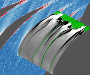
In this section, we focus on the suction-side boundary layer transition. An overview of the instantaneous boundary layer flows for all of the cases is first presented in figure 8, and the vortical structures are shown by iso-surfaces of the  $Q$ criterion (Hunt, Wray & Moin Reference Hunt, Wray and Moin1988). In addition, the contours of the tangential velocity fluctuation
  $u_{t}^{\prime }$ on a surface parallel to the blade are also presented, and the distance between the surface to the blade is around
  $\unicode[STIX]{x1D6FF}/2$ at
  $x=0.5$, with
  $\unicode[STIX]{x1D6FF}$ representing the boundary layer thickness reaching 99 % of the local free-stream mean velocity. It is obvious that the boundary layers show diverse transitional behaviours under the different states of incoming turbulence. For cases with relatively low-level turbulence, i.e. cases A and B, streamwise vortical tubes form in the leading-edge region (
 $x<0.3$) and then stretch downstream in the FPG part of the boundary layer (
 $0.3<x<0.8$). Further downstream, the vortical structures quickly break down into turbulence in the APG region (
 $x>0.8$). At the same time, low-speed streaks, which are considered as dominant structures in bypass transition induced by FST (Durbin & Wu Reference Durbin and Wu2007), are also shown to be present in these cases. For cases C and D featuring increasing amplitude incoming turbulence, the vortical structures are more ‘chaotic’, and the instability and meandering of the low-speed streaks tend to appear farther upstream. Accordingly, the transition onsets occur earlier compared to the cases with lower-level inlet turbulence, which is also shown by the wall-friction coefficient in figure 7(d).

Figure 8. The vortical structures on the suction-side boundary layer: (a) case A; (b) case B; (c) case C; (d) case D. Instantaneous iso-surfaces of  $Q=4000$ are presented, and contours of the tangential velocity perturbations
  $u_{t}^{\prime }$ on a surface parallel to the blade are also shown. The distance between this surface and the blade is around
  $\unicode[STIX]{x1D6FF}/2$ at
  $x=0.5$. In addition, the blue dashed lines indicate the locations of
  $x=0.3$ and
  $x=0.8$.
In the following subsections, the mechanisms for the suction-side boundary layer transition will be discussed, with emphasis on the various phenomena caused by the different FST characteristics. We will first investigate the effects of the blunt leading edge, in which vortical structures start to wrap around the blade and streak-like structures form in the boundary layer. Thereafter, several key mechanisms responsible for the breakdown to turbulence will be presented.

Figure 9. Wall-normal profiles in the leading-edge region. (a) Mean tangential velocity  $U_{t}$ at different locations for case A (lines) and case D (symbols). (b) Velocity fluctuations at the leading edge
  $x=0.0$ for case A (lines and symbols) and case D (symbols only). (c) Mean tangential velocity profiles in wall units for case A (lines) and two-dimensional laminar flow (symbols).
4.1 Leading-edge structures
As shown by the blade geometry in figure 1, the HPT in the present simulations has a blunt leading edge, which is known to have direct effects on the receptivity process of the boundary layer (see Kendall Reference Kendall, Reda, Reed and Kobayashi1991). In addition, it has been reported that streamwise vortices can form around the leading edge, which is due to the tilting and stretching of the incoming wall-normal vortices (Goldstein & Wundrow Reference Goldstein and Wundrow1998; Wundrow & Goldstein Reference Wundrow and Goldstein2001). The streamwise vortices thus can induce wake-like disturbances similar to backward jets (Jacobs & Durbin Reference Jacobs and Durbin2001) or low-speed streaks (Brandt et al. Reference Brandt, Schlatter and Henningson2004), and the instability of these streamwise streaks finally results in the breakdown to turbulence. Other than the instability of streaks, Nagarajan et al. (Reference Nagarajan, Lele and Ferziger2007) introduced a different path to transition considering the effects of the leading edge, for which turbulent spots are formed via precursors which can be traced back to leading-edge structures. This breakdown mechanism due to leading-edge structures was observed to be dominant when the FST intensity or the leading-edge bluntness is large. In the present study, the extraordinarily blunt leading edge of the HPT, along with incoming turbulence of high amplitudes and large scales coming from the inlet, is considered. It is clearly shown in figure 8 that the boundary layer transition taking place in all of the cases is influenced by the vortical structures from the leading-edge region. Therefore, the leading-edge structures will be studied to help understand the downstream transition.
The basic boundary layer statistics, i.e. the profiles of the mean tangential velocity and the velocity fluctuations at different locations, are presented in figure 9. In particular, cases A and D, with the lowest and highest levels of inlet turbulence in the present study, are selected for comparison. As shown in figure 9(a), the mean velocity profiles for both cases are in close agreement with each other, despite the remarkably strong fluctuations to which case D is subjected, as presented in figure 9(b). Furthermore, the mean tangential velocity profiles in case A are plotted in wall units in figure 9(c), in comparison with the profiles from a two-dimensional case without any FST, and the close agreement implies that the boundary layers in the leading-edge region ( $x<0.3$) stay laminar. This is due to the stabilizing effects of the strong FPG and high convex curvature (see Muck, Hoffmann & Bradshaw Reference Muck, Hoffmann and Bradshaw1985; Katz, Seifert & Wygnanski Reference Katz, Seifert and Wygnanski1990; Mukund et al. Reference Mukund, Viswanath, Narasimha, Prabhu and Crouch2006), which are prominent in the leading-edge region as identified in figure 7(b,c).
It is also demonstrated in figure 9 that compared to other components, the amplitude of the spanwise fluctuation is much larger near the wall in both cases. The strong spanwise disturbances at the leading edge are also shown by instantaneous contours of the spanwise velocity component in figure 10(a), and a schematic for this plane cut is given in figure 10(b). It appears that the large amplitude of tangential vorticity, presented by the iso-lines, is basically located at those regions showing strong gradients of the spanwise velocity fluctuation  $w^{\prime }$. This relation between the large amplitude of spanwise disturbances and tangential vorticity can be expressed as
  $\unicode[STIX]{x1D714}_{t}^{\prime }\sim \unicode[STIX]{x2202}w^{\prime }/\unicode[STIX]{x2202}n$, with
  $n$ representing the wall-normal distance to the blade surface. Similar to the observation in Goldstein & Wundrow (Reference Goldstein and Wundrow1998), the tangential vortices at the leading edge will wrap around the blade surface, and the resulting streamwise vortices are expected to play a key role in downstream transition.

Figure 10. (a) Contour of spanwise velocity fluctuation at the leading-edge wall-normal plane cut in case A. Iso-lines of tangential vorticity  $\unicode[STIX]{x1D714}_{t}^{\prime }$ (normal to the plane cut) are also shown, with solid and dashed lines indicating
  $\unicode[STIX]{x1D714}_{t}^{\prime }=100$ and
  $\unicode[STIX]{x1D714}_{t}^{\prime }=-100$, respectively. (b) Schematic for the wall-normal plane cut at the leading edge.
The effects of the leading-edge structures on the boundary layer are further investigated by scrutinizing flow variables in the wall-normal–spanwise planes, as shown in figure 11. In the wall-normal plane cut near the suction peak at  $x=0.3$, the iso-lines of
  $Q$ represent the streamwise vortical structures wrapped around the leading edge, which are also shown in figure 8, while the contours show the tangential velocity fluctuation
  $u_{t}^{\prime }$ and the temperature fluctuation
  $T^{\prime }$. For case A, it is noted that the near-wall region as marked by the black dashed box in figure 11(a) is packed with strips of positive and negative velocity fluctuations. In particular, the low-speed fluid seems to be elevated and forms ‘mushroom-like’ structures, which are also shown by the contour of temperature fluctuation
  $T^{\prime }$ from figure 11(c). The lift-up effects of the vortical structures are clearly presented in figure 11(d,e), in which two ‘mushroom-like’ structures in figure 11(c) are extracted to provide a zoom-in view, with the vectors showing the velocity fluctuations in the spanwise
  $w^{\prime }$ and wall-normal
  $u_{n}^{\prime }$ directions. It appears that the vortical structures induce strong upward velocity near the wall, driving the fluid with relatively low temperature away from the blade and thus enhancing the heat flux. Therefore, the streamwise vortices are proven to be directly linked to the low-speed streaks, which has also been presented in several previous studies on flat-plate boundary layers with zero pressure gradients (Andersson et al. Reference Andersson, Brandt, Bottaro and Henningson2001).

Figure 11. Instantaneous snapshots for contours of spanwise and wall-normal plane cuts at  $x=0.3$: (a) tangential velocity fluctuation
  $u_{t}^{\prime }$ for case A; (b)
  $u_{t}^{\prime }$ for case D; (c) temperature fluctuation
  $T^{\prime }$ for case A; (d,e) zoom-in views of ‘mushroom-like’ structures of
  $T^{\prime }$ with fluctuating velocity vectors. The iso-lines of
  $Q=4000$ are also presented in the contours. Note that the wall-normal coordinate
  $n$ is enlarged to clearly show the structures.
For comparison, the contour of  $u_{t}^{\prime }$ in figure 11(b) shows the velocity fluctuations in case D, which are apparently much more violent compared to those in case A. Moreover, the iso-lines of
  $Q$ are nearly randomly distributed over the plane cut, corresponding to the ‘chaotic’ vortical structures as shown in figure 8(d). This indicates that the high-level FST in case D drives stronger fluctuations and thus ‘chaotic’ vortical structures in the boundary layer, which are expected to cause much earlier transition as presented in figure 7(d). The different states of the vortical structures obviously cause different paths of transition, and the details will be further discussed in § 4.2.

Figure 12. Instantaneous snapshots for streaks and the breakdown to turbulence at  $t=t_{0}$ in case A. Contours of (a) streamwise component
  $u_{t}^{\prime }$, (b) wall-normal
  $u_{n}^{\prime }$ and (c) spanwise
  $w^{\prime }$ are presented at the surface which is
  $n=\frac{1}{2}\unicode[STIX]{x1D6FF}(x=0.5)$ from the wall. The blue dashed line indicates the boundary between FPG and APG at
  $x=0.8$, and an incipient turbulent spot is highlighted by the red dotted circle.
4.2 Breakdown mechanisms
Affected by the structures formed at the leading-edge region and the continuing exposure to the FST, the suction-side boundary layers in the present simulations show differences in their transition behaviours, e.g. different transition onsets indicated by the wall-friction coefficient in figure 7(d) and various structures shown in figure 8. In this section, we will investigate the various transition mechanisms, including the instability of streaks in the cases with relatively low-level incoming turbulence, and the breakdown caused by vortical structures in the case with higher-level turbulence.
4.2.1 Varicose breakdown
With the relatively low-level turbulence in cases A and B, the boundary layers show elongated streaks across the FPG region as presented in figure 8(a,b), and the transition onset is near the blade trailing edge under the APG. In figure 12, another view of the suction-side boundary layer for case A is given, displaying the contours of  $u_{t}^{\prime }$,
  $u_{n}^{\prime }$ and
  $w^{\prime }$ on a surface at a distance of
  $\unicode[STIX]{x1D6FF}(x=0.5)$ from the wall. The low- and high-speed streaks in the streamwise direction can be shown by the
  $u_{t}^{\prime }$ contour. It is also apparent that for the streamwise streaks in the suction-side boundary layer, the tangential velocity fluctuation
  $u_{t}^{\prime }$ is much stronger than the other components. These streaks, which are usually considered as key features in bypass transition (Durbin & Wu Reference Durbin and Wu2007), are closely related to the lift-up effects of the streamwise vortical structures formed at the leading edge (Andersson et al. Reference Andersson, Brandt, Bottaro and Henningson2001).
The instability of the streaks in the APG region, as highlighted by the red dashed circle in figure 12, is more clearly shown by the wall-normal and spanwise velocity fluctuations, and it is further studied in a zoom-in view in figure 13. Corresponding to the snapshot in figure 12 at  $t=t_{0}$, the contour of
  $u_{n}^{\prime }$ in figure 13(a) shows a symmetric distribution about the streamwise direction. In addition, the iso-lines of
  $w^{\prime }$ are also presented, showing an antisymmetric pattern, with solid lines and dashed lines indicating
  $w^{\prime }=0.2$ and
  $w^{\prime }=-0.2$, respectively. It is noted that although the symmetry presented in figure 13(a) is not perfect due to the strong upstream turbulence, this type of instability corresponds well with varicose or symmetric modes (Andersson et al. Reference Andersson, Brandt, Bottaro and Henningson2001; Asai, Minagawa & Nishioka Reference Asai, Minagawa and Nishioka2002).

Figure 13. Zoom-in view of the instability of the streak in case A indicated by the red circle in figure 12. Instantaneous snapshots are presented at (a)  $t=t_{0}$, (b)
  $t=t_{0}+0.0115$ and (c)
  $t=t_{0}+0.023$, with
  $t_{0}$ representing the snapshot shown in figure 12. Contours of the wall-normal velocity fluctuation
  $u_{n}^{\prime }$ are presented on the surface
  $\unicode[STIX]{x1D6FF}/2$ away from the wall, and the iso-lines of spanwise velocity fluctuation
  $w^{\prime }$ are also shown, with solid lines and dashed lines indicating
  $w^{\prime }=0.2$ and
  $w^{\prime }=-0.2$, respectively.

Figure 14. The inception of the varicose mode instability of the streak indicated by the red circle in figure 12. The contours of the tangential velocity perturbations  $u_{t}^{\prime }$ on a cross-spanwise plane cut across the streak are shown by the instantaneous snapshots at (a)
  $t=t_{0}-0.023$, (b)
  $t=t_{0}-0.0115$, (c)
  $t=t_{0}$ and (d)
  $t=t_{0}+0.0115$, with
  $t_{0}$ representing the snapshot shown in figure 12. The iso-surfaces of
  $u_{t}^{\prime }=1.0$ (red),
  $u_{t}^{\prime }=-1.0$ (blue) and
  $Q=4000$ (green) are also shown at (e)
  $t=t_{0}-0.023$, (f)
  $t=t_{0}-0.0115$, (g)
  $t=t_{0}$ and (h)
  $t=t_{0}+0.0115$.
The inception of the varicose instability, which was found to be driven by the wall-normal shear of the streamwise flow by Skote et al. (Reference Skote, Haritonidis and Henningson2002), can be represented by the contours of  $u_{t}^{\prime }$ on a cross-spanwise plane cut across the streak. In figure 14(a–d), the snapshots are from a sequence of time instants at
  $t_{0}-2\unicode[STIX]{x0394}t$,
  $t_{0}-\unicode[STIX]{x0394}t$,
  $t_{0}$ and
  $t_{0}+\unicode[STIX]{x0394}t$, respectively, with
  $t_{0}$ corresponding to the snapshot shown in figure 12 and
  $\unicode[STIX]{x0394}t=0.0115$. It is clearly shown that the varicose instability here happens due to the interactions between the low- and high-speed streaks (Brandt et al. Reference Brandt, Schlatter and Henningson2004; Lundell & Alfredsson Reference Lundell and Alfredsson2004). Specifically, the fast-moving high-speed streak reaches the downstream low-speed region, and the instability is triggered at the interface in between. This instability grows rapidly at the tilting interface between the streaks, particularly with the presence of the APG which enhances the inflection for the streamwise velocity profiles. The development of the varicose mode instability can be further shown by the iso-surfaces of
  $u_{t}^{\prime }$ in figure 14(e–h), highlighting the formation of the vortical structures represented by the
  $Q$ iso-surface. Convecting downstream, the streaks quickly break down as also suggested by the contours at two subsequent snapshots at
  $t_{0}+\unicode[STIX]{x0394}t$ and
  $t_{0}+2\unicode[STIX]{x0394}t$ in figure 13(b,c).
4.2.2 Sinuous breakdown
For case C with higher-amplitude incoming turbulence, early-stage turbulent spots are observed in the FPG region, while the skin friction indicates that the mean flow stays laminar. In figure 15, a sequence of the contours of wall-normal velocity fluctuation  $u_{n}^{\prime }$ is shown to track the formation of a turbulent spot, with the evolution of the spanwise-averaged wall-friction coefficient
  $C_{f}$ for the corresponding snapshots also plotted on the suction-side surface. The contour surface is inside the boundary layer, at a distance of
  $\unicode[STIX]{x1D6FF}/2$ away from the wall, where
  $\unicode[STIX]{x1D6FF}$ is the boundary layer thickness at
  $x=0.5$. In these snapshots, the spot precursor first stretches in the streamwise direction from figures 15(a) to 15(b). As the amplitude of the disturbances is still small, the variation of the
  $C_{f}$ value near the spot is nearly negligible. Travelling downstream, the disturbances rapidly amplify and the precursor starts to break down, with the
  $C_{f}$ value around the spot significantly increasing as shown in figure 15(c). Specifically, the breakdown of the spot precursor initiates at the tail and expands in the spanwise direction, resulting in a triangular shape, with the head towards the downstream direction. The spot continues to grow in both size and amplitude moving further downstream, which can be shown by the evolution of the
  $C_{f}$ wave-packet indicated by the blue arrow. Nevertheless, it is noted that the skin friction recovers to the undisturbed state again once the spot has passed by, suggesting that the disturbances for the formation and evolution of the turbulent spot are localized and there are calming effects trailing the spot. The temporal evolution of the displacement thickness of the boundary layer at
  $x=0.8$, which is indicated by the blue dashed line in figure 15, is presented in figure 16, showing that the displacement thickness relaxes to a value even smaller than that in the undisturbed state after the spot-caused peak. As suggested by Katz et al. (Reference Katz, Seifert and Wygnanski1990), the low displacement thickness trailing the turbulent spot indicates the existence of a calmed region which is presumably caused by the distortion of the local mean flow by some nonlinear process. Finally, the enlarged spot merges with the turbulent boundary layer near the blade trailing edge, while a new spot precursor forms in the FPG region again as shown in figure 15(e).

Figure 15. Formation of the turbulent spot in case C. Contours of wall-normal velocity fluctuation  $u_{n}^{\prime }$ at the instantaneous snapshots (a)
  $t=t_{0}$, (b)
  $t=t_{0}+0.069$, (c)
  $t=t_{0}+0.138$, (d)
  $t=t_{0}+0.207$ and (e)
  $t=t_{0}+0.276$. The blue dashed lines indicate
  $x=0.3$ and
  $x=0.8$, respectively, and the spot precursor is highlighted by the red dashed circle. Meanwhile, the wall-friction coefficient
  $C_{f}$ on the suction-side surface is averaged in the spanwise direction and plotted against
  $x$ for the corresponding snapshots (red solid lines), with the mean
  $C_{f}$ represented by the black dashed lines for reference.

Figure 16. Temporal evolution of the displacement thickness of the boundary layer profile at  $x=0.8$ in case C. The instantaneous profile is spanwise-averaged, starting from
  $t_{0}$ corresponding to figure 15(a).
In order to further investigate the incipient spot, a zoom-in view of the spot precursor is shown in figure 17, tracking the structures highlighted by the red dashed circle in the snapshots of figure 15(a–c). Here, the vortical structures are identified by the iso-surface of  $Q$ in figure 17(a–c), and the iso-surfaces of
  $u_{t}^{\prime }$ are also shown to track the development of the streamwise velocity fluctuation streaks. It is shown in figure 17(a,d) that there exists a quasi-streamwise vortex filament located in the strong spanwise shear region between the low- and high-speed streaks. The streamwise-elongated vortex filament, which seems to be a remnant of the leading-edge vortical structures, is tilting with the wall-normal vorticity component
  $\unicode[STIX]{x1D714}_{n}^{\prime }\sim \unicode[STIX]{x2202}u_{t}^{\prime }/\unicode[STIX]{x2202}n$. A secondary instability of the streak is then observed, caused by the strong spanwise shear in figure 17(b,e), with the tail of the filament oscillating in the spanwise direction. Furthermore, the streak breaks down and forms the triangular spot seen in figure 17(c,f).

Figure 17. Zoom-in view of the instantaneous structures highlighted by the red dashed circle in figure 15 to show the breakdown in case C. Contours of the streamwise velocity fluctuation  $u_{t}^{\prime }$ are shown on the surface at
  $\unicode[STIX]{x1D6FF}/2$ from the wall, and iso-surface of
  $Q=4000$ is also shown at (a)
  $t=t_{0}$, (b)
  $t=t_{0}+0.069$ and (c)
  $t=t_{0}+0.138$. Iso-surfaces of
  $u_{t}^{\prime }=1.0$ (red) and
  $u_{t}^{\prime }=-1.0$ (blue) at (d)
  $t=t_{0}$, (e)
  $t=t_{0}+0.069$ and (f)
  $t=t_{0}+0.138$.
It is noted that the spanwise oscillations observed in figure 17(b) are only on one side of the streak, which is in close agreement with the one-sided sinuous mode. As discussed by Brandt et al. (Reference Brandt, Schlatter and Henningson2004), the sinuous instability of low-speed streaks, though many are symmetric, can be dominated by single-direction vorticity and oscillate only in one direction. This one-sided instability is believed to be related to the spanwise asymmetry of the streaks, which is indeed present for case C with strong FST. Furthermore, contours of the streamwise velocity fluctuation  $u_{t}^{\prime }$ in four cross-stream plane cuts at different streamwise positions, which correspond to the sinuous disturbances in figure 17(b), are shown in figure 18. Along with the vectors showing the fluctuating velocities in the wall-normal and spanwise directions, the meandering of the low-speed streak also gives further credibility to the hypothesis of the presence of a one-sided instability.

Figure 18. The inception of the varicose mode instability in case C, corresponding to the snapshot shown in figure 17(b) at the instantaneous snapshot  $t=t_{0}+0.069$. The contours of the tangential velocity perturbations
  $u_{t}^{\prime }$ are shown on four cross-streamwise plane cuts between the two blue dashed lines in figure 17(b) at (a)
  $x=0.70$, (b)
  $x=0.705$, (c)
  $x=0.71$ and (d)
  $x=0.715$, and the vectors present the fluctuating velocities on the plane.

Figure 19. Formation of the turbulent spot in case D. Contours of wall-normal velocity fluctuation  $u_{n}^{\prime }$ at the instantaneous snapshots (a)
  $t=t_{0}$, (b)
  $t=t_{0}+0.046$, (c)
  $t=t_{0}+0.092$ and (d)
  $t=t_{0}+0.138$. The blue dashed lines indicate
  $x=0.5$ and
  $x=0.8$, respectively, and the spot precursor is highlighted by the red dashed circle.
4.2.3 Breakdown induced by vortex interaction
For case D, the velocity fluctuations in the boundary layer are stronger than in other cases and the vortical structures are more ‘chaotic’ from the blade leading edge, as shown in figure 11. As a result, the transition onset shown by skin friction already occurs in the FPG region ( $x<0.8$) for case D, which is much earlier than in the other cases. In order to investigate the transition mechanisms, the breakdown process is presented by the contours of the wall-normal velocity fluctuations
  $u_{n}^{\prime }$ in figure 19. As a result of the large-amplitude inlet turbulence, the contours of
  $u_{n}^{\prime }$ for case D show much stronger fluctuations, compared to case C shown in figure 15, that has the same turbulence amplitude at the inlet but a smaller length scale and thus exhibits more rapid decay of the incoming turbulence. In particular, once the flow enters into the region with relatively weak FPG and convex curvature, which is downstream of the first blue dashed line representing
  $x=0.5$, the fluctuations originating from the leading edge induce multiple structure breakdowns in the spanwise extent. One spot precursor, as highlighted by the red dashed circle in figure 19, is considered as an example and tracked through the formation process. The precursor is first observed just downstream of
  $x=0.5$, and it rapidly grows in size in both the streamwise and spanwise directions, travelling downstream. Thereafter, while the precursor breaks down to form a region packed with smaller-scale fluctuations, the shape of this region is obviously different from the spot shown in figure 15.
The formation of the spot is further investigated in the zoom-in view presented in figure 20, with the vortical structures identified by the iso-surface of the  $Q$ criterion and the contours of
  $u_{t}^{\prime }$ also shown. The instability of streaks, as presented for cases A, B and C in §§ 4.2.2 and 4.2.1, is not clearly observed here. Rather, the spot precursor results from the vortical breakdown. The pair of vortex filaments, as highlighted by the blue dashed circle in figure 20(a), forms a
  $\unicode[STIX]{x1D6EC}$-shape with the tip pointing in the negative streamwise direction, which is the opposite from the
  $\unicode[STIX]{x1D6EC}$-like structures usually observed in natural transition (Zhao, Yang & Chen Reference Zhao, Yang and Chen2016a,Reference Zhao, Yang and Chenb; Zhao et al. Reference Zhao, Xiong, Yang and Chen2018). The resulting spot, as presented in figure 20(b), is therefore different from the ordinary turbulent spots with the head towards the downstream direction, as shown in figure 17(c).

Figure 20. Zoom-in view of the instantaneous structures highlighted by the red dashed circle in figure 19 to show the breakdown in case D, at (a)  $t=t_{0}$ and (b)
  $t=t_{0}+0.046$. Contours of the streamwise velocity fluctuation
  $u_{t}^{\prime }$ are shown on the surface at
  $\unicode[STIX]{x1D6FF}/2$ from the wall, and iso-surfaces of
  $Q=4000$ are also shown.

Figure 21. The incipient of the spot in case D. The contours of the instantaneous tangential velocity perturbations  $u_{t}^{\prime }$ on a cross-spanwise plane cut at
  $z=0.29$ as indicated by the blue dashed arrow in figure 20: (a)
  $t=t_{0}$, (b)
  $t=t_{0}+0.023$, (c)
  $t=t_{0}+0.046$ and (d)
  $t=t_{0}+0.069$, with
  $t_{0}$ representing the snapshot shown in figure 20(a). The window is moving at a speed of
  $c=1.74$ to track the spot precursor highlighted by the blue dashed circle in figure 20(a).
The breakdown of the precursor highlighted in figure 20(a) can be further shown by the contours of  $u_{t}^{\prime }$ in the cross-spanwise plane cut at the tip of the precursor. In figure 21(a), the tip of the
  $\unicode[STIX]{x1D6EC}$-shaped vortex pair is located at the interface between the high- and low-speed region, as indicated by the black solid arrow. The vortex pair induces a downward movement of relatively high-speed fluid and elevates the upstream low-speed fluid from the wall, and the instability of the interface rapidly develops and then breaks down under the strong background turbulence, as shown in the subsequent snapshots in figure 21(b–d).
We remark here that the  $\unicode[STIX]{x1D6EC}$-shaped vortex in figure 20(a) is just one example of the key structures. Due to the ‘chaotic’ nature of the vortical structures under the strong background turbulence, structures of different forms have also been identified in the formation of spot precursors in case D. The consistent mechanism for this type of breakdown, however, is that the precursors always originate from energetic vortical structures that can be traced back to the blade leading edge. The transition breakdown resulting from leading-edge structures seems to be in close agreement with the leading-edge effects discussed in Nagarajan et al. (Reference Nagarajan, Lele and Ferziger2007), in which the vortical effect is dominant when the bluntness is large and the FST is strong.
As a summary, the transition onsets in cases A and B are in the APG region close to the blade trailing edge. High- and low-speed streaks are observed, which are induced by the lift-up effects of the streamwise vortices formed at the leading edge. The structures then transform while convected downstream, due to a varicose mode instability that occurs as a result of the wall-normal inflectional instability under the APG, and which rapidly amplifies and causes the final breakdown to turbulence. For cases with stronger FST, however, the transition onsets occur much earlier. For case C, spot precursors form in the weak FPG region, and the formation process is through the secondary instability of streaks, which is observed to be the sinuous mode. Furthermore, with the even stronger FST entering the HPT cascade in case D, the vortical structures formed at the leading edge are in a chaotic manner and have a direct effect on the transition breakdown.
5 Discussion on effects of incoming turbulence
In this section, we will summarize the effects of the inlet turbulence on transition mechanisms in the present cases in which the suction-side boundary layers are subject to pressure gradients and surface curvature, and the results will be compared to those of previous studies which have predominantly focused on flat-plate boundary layers with zero pressure gradient.
First of all, the effects of the turbulence length scales, in addition to the resulting different decay rate as presented in figure 4(a), are analysed by comparing the transitional structures in cases A and B. It is noted that cases A and B have significantly different integral length scales of the incoming turbulence, as shown in figure 4(b), while the turbulence intensities upstream of the leading edge ( $x=-0.2$) are relatively close to each other with
  $T_{u}=6.1\,\%U_{in}$ and
  $5.2\,\%U_{in}$, respectively. The transition onsets agree well with each other as observed in figure 7(d), and streak-like structures and their instability are observed in both cases A and B as discussed in § 4.2.1. Therefore, a qualitative comparison between cases A and B implies that the transition mechanisms in relatively low-level FST cases are not directly influenced by the significant difference in integral length scales. Considering cases C and D which show distinctive levels of turbulence upstream of the leading edge (
 $T_{u}=16.8\,\%U_{in}$ and
  $9.5\,\%U_{in}$ at
  $x=-0.2$) and thus significantly different transitional behaviours as discussed in § 4, the leading factor dominating the transition behaviours in the present cases seems to be whether the turbulence intensity is strong enough to overcome the stabilizing effect of the FPG.
However, a quantitative analysis is still needed to answer one open question – whether the length scales of the FST affect the scales of the transitional structures, especially the streamwise streaks in the boundary layer. In previous studies of bypass transition in flat-plate boundary layers, the spanwise spacing of the streaks induced by FST was usually observed in experiments to be at the scale of the boundary layer thickness (Matsubara & Alfredsson Reference Matsubara and Alfredsson2001), and it was reported in numerical simulations (Brandt et al. Reference Brandt, Schlatter and Henningson2004) that the spanwise scale of the streaks is only weakly dependent on the scale of the disturbance in the free stream. Also, these are in accordance with the theoretical results of Luchini (Reference Luchini2000) and Andersson et al. (Reference Andersson, Berggren and Henningson1999), which show an optimal scale of 1.4 times the boundary layer thickness on a flat surface. On the other hand, Ovchinnikov et al. (Reference Ovchinnikov, Choudhari and Piomelli2008) reported that the FST length scale can affect not only the onset of transition, but also the underlying physical mechanism including the critical vortical structures and spacing of the streaks. More recently, the importance of the integral length scales for predicting transition onset is stressed based on the experimental data consisting of 42 FST states (Fransson Reference Fransson2017).

Figure 22. (a) Spanwise correlation of the tangential velocity fluctuation  $u_{t}^{\prime }$ on the suction-side boundary layer at
  $x=0.5$. (b) Development of the spanwise spacing of the streaks
  $\unicode[STIX]{x1D6E5}_{z}$ compared to the local boundary layer thickness
  $\unicode[STIX]{x1D6FF}$, and spacing normalized in the local wall units
  $\unicode[STIX]{x1D6E5}_{z}^{+}$.
In the present study, the spanwise spacings of the streaks in cases A and B, quantified by twice the distance to the minimum of the spanwise correlations of  $u_{t}^{\prime }$ shown in figure 22(a), are compared with the local boundary layer thickness. As becomes evident from figure 22(b), the spanwise spacings at the suction peak
  $x=0.3$ in cases A and B are
  $\unicode[STIX]{x1D6E5}_{z}=0.058$ and 0.18, respectively, which are of the order of the integral length scales from the inlet turbulence and much larger than the boundary layer thickness. Furthermore, the spanwise spacings of the streaks slightly increase in the FPG boundary layer, corresponding to the growth of the streaks in both size and intensity. We thus conclude here that the spanwise spacings of the streaks in the present study depend on the FST and are not directly connected to the boundary layer thickness. It is also interesting to compare the present streaks in the transitional boundary layers with the well-known streaks as key coherent structures in fully turbulent boundary layers. The spanwise spacing of wall-turbulence streaks was found to exhibit consistent values of
  $\unicode[STIX]{x1D6E5}_{z}^{+}\approx 100$ in the near-wall region (Smith & Metzler Reference Smith and Metzler1983) and can go as high as
  $\unicode[STIX]{x1D6E5}_{z}^{+}\approx 1500$ in the outer layer (Jiménez Reference Jiménez2018), while the spanwise spacings of the streaks in the present study, normalized in wall units, are
  $\unicode[STIX]{x1D6E5}_{z}^{+}\approx 1000{-}1500$ in case A and
  $\unicode[STIX]{x1D6E5}_{z}^{+}\approx 3000{-}4000$ in case B. Moreover, Brinkerhoff & Yaras (Reference Brinkerhoff and Yaras2015) found in a numerical simulation of a flat-plate boundary layer with pressure gradient that although the stabilizing effects of a FPG can cause a larger streak spacing in wall units, resulting in typical spacing of
  $\unicode[STIX]{x1D6E5}_{z}^{+}\approx 198$, the streak spacing seems to be at the scale of the local boundary layer thickness with the existence of acceleration. Therefore, considering the much larger streak spacing compared to the local boundary layer thickness found in the current work, and the significant variations of streak spacings in cases A and B, it is likely that the streaks here mainly originate from the vortical structures formed at the blunt blade leading edge as a consequence of the incoming turbulence, rather than through a scale selection of the boundary layer.
The development of the fluctuations in the boundary layer can be characterized by the wall-normal maximum of the tangential velocity fluctuation  $\max _{n}(u_{t}^{\prime })^{2}$. As shown in figure 23(a),
  $\max _{n}(u_{t}^{\prime })^{2}$ in case A first decreases due to the large-amplitude curvature and the strong pressure gradient, as indicated in figure 7(b,c). Downstream of
  $x=0.5$, the curvature effect and the FPG turn much weaker, and the streamwise streaks start growing. As a comparison, figure 23(b) shows that the spanwise component
  $\max _{n}(w^{\prime })^{2}$ monotonically decreases until the transition onset, after which the growth rate of
  $\max _{n}(u_{t}^{\prime })^{2}$ also significantly increases. This suggests that the streamwise streaks in the boundary layer are dominated by the fluctuations in the streamwise direction, and the strength of the streaks keeps increasing for the weak FPG and APG regions.

Figure 23. Development of the wall-normal maximum of the streamwise velocity fluctuation.
In addition, the effects of the inlet turbulence can be studied by comparing results between all the cases. It is shown that compared to cases A, B and C, the growth rate of  $\max _{n}(u_{t}^{\prime })^{2}$ in case D is much larger and the spanwise fluctuations are apparently much stronger, which is in accordance with the structures being more chaotic and consistent with the fact that a different path from streak instability is responsible for the transition. Furthermore, for cases A, B and C which show obvious streak instabilities during transition, the growth rates in the weakly FPG region (from
  $x=0.5$ to
  $x=0.8$) are compared in figure 23(c), showing that
  $\max _{n}(u_{t}^{\prime })^{2}$ grows approximately linearly with the Reynolds number based on the surface distance
  $Re_{s}$. This observation agrees with previous experimental (Kendall Reference Kendall1985; Matsubara & Alfredsson Reference Matsubara and Alfredsson2001) and theoretical (Andersson et al. Reference Andersson, Berggren and Henningson1999; Luchini Reference Luchini2000) results obtained for flat-plate boundary layers with zero pressure gradient. Furthermore, the algebraic growth of streaks was also observed in the flat-plate boundary layer simulation with pressure gradient by Brinkerhoff & Yaras (Reference Brinkerhoff and Yaras2015), in which the variation of FPG seems to not affect the growth rate. The differences observed in the present cases compared to the flat-plate boundary layer in Brinkerhoff & Yaras (Reference Brinkerhoff and Yaras2015), especially the strong stabilizing effects causing the decrease of the streak intensity at
  $x<0.5$ as shown in figure 23(a), highlight the influence of the strong FPG and convex curvature of the blunt leading edge. To summarize, even though the streamwise streaks in the present cases are mainly induced by the vortical structures formed near the leading-edge region, and thus have spanwise scales much larger than the local boundary layer thickness, the growth of the streaks at the downstream stage with weak pressure gradient and curvature is still closely related to the algebraic or transient growth theory. Moreover, it is shown that the growth rates of
  $\max _{n}(u_{t}^{\prime })^{2}$ in cases with stronger FST are slightly larger, implying that the growth of the streaks is also affected by the FST (Asai et al. Reference Asai, Konishi, Oizumi and Nishioka2007).
The development of the velocity fluctuations along the suction-side boundary layer can be further characterized by the spanwise spectra, as presented in figure 24. The spectra in the streamwise  $\hat{u} _{t}^{\prime }$, the wall-normal
  $\hat{u} _{n}^{\prime }$ and the spanwise
  ${\hat{w}}^{\prime }$ directions are obtained as
 $$\begin{eqnarray}\hat{u} _{i}^{\prime }(x,k_{z})={\mathcal{F}}_{z}\{u_{i}^{\prime }(x,z)\},\end{eqnarray}$$
 where  ${\mathcal{F}}_{z}$ represents the Fourier transform in the spanwise direction. In figure 24, the time-averaged spectra
  $\langle |\hat{u} _{i}^{\prime }(x,k_{z})|^{2}\rangle$ for case A are plotted against
  $x$ at the surface which is
  $\frac{1}{2}\unicode[STIX]{x1D6FF}(x=0.5)$ from the wall, and case D with much higher levels and greater length scales of FST is presented for comparison. It is apparent that the velocity fluctuations are mainly at low wavenumbers before the boundary layer transitions into turbulence, which suggests the boundary layer is predominately affected by the large-scale part of the FST. After transition, the high-wavenumber amplitudes for all of the components significantly amplify, and the spectra become broadband. Furthermore, the streamwise fluctuating velocity is shown to be dominant for most of the boundary layer, while the wall-normal component
  $\langle |\hat{u} _{n}^{\prime }(x,k_{z})|^{2}\rangle$ is negligible, until transition to turbulence has occurred. The spanwise component
  $\langle |{\hat{w}}^{\prime }(x,k_{z})|^{2}\rangle$, however, is prevailing in the leading-edge region, but the amplitude gradually decreases in the FPG region (
 $x<0.8$). This is presumably due to the stabilizing effects of the FPG and the convex surface. Compared to case A, the transition in case D takes place much earlier due to the higher-amplitude FST. This is also shown in figure 8(d–f), in which the spectra of fluctuating velocities in case D turn broadband at around
  $x=0.8$.

Figure 24. The evolution of the spanwise spectra of the fluctuating velocities along the suction side of the blade. The spectra of the velocity components are extracted at the surface which is  $n=\frac{1}{2}\unicode[STIX]{x1D6FF}(x=0.5)$ from the wall and plotted against the streamwise coordinate
  $x$ and spanwise wavenumber
  $k_{z}$. The contours are (a)
  $\langle |\hat{u} _{t}^{\prime }(x,k_{z})|^{2}\rangle$ in case A, (b)
  $\langle |\hat{u} _{n}^{\prime }(x,k_{z})|^{2}\rangle$ in case A, (c)
  $\langle |{\hat{w}}^{\prime }(x,k_{z})|^{2}\rangle$ in case A, (d)
  $\langle |\hat{u} _{t}^{\prime }(x,k_{z})|^{2}\rangle$ in case D, (e)
  $\langle |\hat{u} _{n}^{\prime }(x,k_{z})|^{2}\rangle$ in case D and (f)
  $\langle |{\hat{w}}^{\prime }(x,k_{z})|^{2}\rangle$ in case D.
In addition, it is worth noting that one peak of the  $\langle |\hat{u} _{t}^{\prime }(x,k_{z})|^{2}\rangle$ spectrum in the leading-edge region is shown by the red arrow in figure 24(a), which indicates a wavelength of
 $$\begin{eqnarray}\unicode[STIX]{x1D706}_{z}=\frac{2\unicode[STIX]{x03C0}}{k_{z}}\approx 0.058.\end{eqnarray}$$
 This wavelength corresponds to the spanwise spacing of the low-speed streaks at the leading-edge region  $x=0.3$ in case A, as also observed in figure 22(b).
6 Conclusions
In the present study, large-eddy simulations of an HPT at realistic Reynolds and Mach numbers have been performed, and the inlet turbulence was varied in four cases to study the effects of turbulence intensities and length scales on the boundary layer transition. Due to the interactions between the incoming turbulence and the blunt blade leading edge, vortical structures wrap around the leading edge and thus affect the boundary layer transition on the suction side. For cases with different FST, various paths for transition are observed, including the sinuous and varicose modes of streak instability and the breakdown caused by vortical interactions.
In cases with relatively low-level turbulence, i.e. cases A, B and C, the low- and high-speed streaks are observed to originate from the leading-edge vortical structures, and the spanwise length scales of the streaks are related to the integral length scales of the upstream turbulence. While the streaks are mainly induced by the leading-edge vortical structures and subject to FPG and curvature effects, the boundary layer fluctuations grow linearly with  $Re_{s}$, which is in close agreement with the algebraic or transient growth originally proposed in a flat-plate boundary layer with zero pressure gradient. Furthermore, the streaks break down and the transition onsets are through the instability of the streaks, either the varicose mode in the APG region or the sinuous mode earlier in the weak FPG region. For cases with higher levels of FST, however, the leading-edge structures are more chaotic and no obvious streak instability is observed. Accordingly, the transition onset occurs much earlier on the suction side, through a breakdown caused by interactions between vortical structures.
Acknowledgements
This research used resources of the Oak Ridge Leadership Computing Facility, which is a DOE Office of Science User Facility supported under contract DE-AC05-00OR22725. This work was also supported by the resources provided by the Pawsey Supercomputing Centre with funding from the Australian Government and the Government of Western Australia. This work was also supported by a grant from the Swiss National Supercomputing Centre (CSCS) under project ID s884.
Declaration of interests
The authors report no conflict of interest.


