2.1 Hydrostatic Boussinesq dynamics on the $f$-plane

Our starting point is the 3-D Boussinesq, hydrostatic equations with traditional approximation for the Coriolis force (Vallis Reference Vallis2017). This is a standard model for geophysical flows, including the effect of rotation and stratification through the Coriolis parameter $f$ (twice the projection of the planet rotation rate on the local vertical axis) and the buoyancy frequency $N$. Calling $L$ and $H$ the typical horizontal and vertical length scales of the flow, respectively, with typical velocity $U$, the Boussinesq dynamics admits three non-dimensional parameters: the aspect ratio, the Rossby number and the Burger number, defined as

(2.1a-c)$$\begin{eqnarray}\unicode[STIX]{x1D6FC}\equiv \frac{H}{L},\quad Ro\equiv \frac{U}{Lf},\quad Bu\equiv \left(\frac{NH}{fL}\right)^{2}.\end{eqnarray}$$

The hydrostatic limit corresponds to $\unicode[STIX]{x1D6FC}\ll 1$. The hydrostatic Boussinesq system is

(2.2)$$\begin{eqnarray}\displaystyle & \unicode[STIX]{x2202}_{x}u+\unicode[STIX]{x2202}_{y}v+\unicode[STIX]{x2202}_{z}w=0, & \displaystyle\end{eqnarray}$$

(2.3)$$\begin{eqnarray}\displaystyle & 0=-\unicode[STIX]{x2202}_{z}p+b, & \displaystyle\end{eqnarray}$$

(2.4)$$\begin{eqnarray}\displaystyle & Ro(\unicode[STIX]{x2202}_{t}+u\unicode[STIX]{x2202}_{x}+v\unicode[STIX]{x2202}_{y}+w\unicode[STIX]{x2202}_{z})u=-\unicode[STIX]{x2202}_{x}p+v, & \displaystyle\end{eqnarray}$$

(2.5)$$\begin{eqnarray}\displaystyle & Ro(\unicode[STIX]{x2202}_{t}+u\unicode[STIX]{x2202}_{x}+v\unicode[STIX]{x2202}_{y}+w\unicode[STIX]{x2202}_{z})v=-\unicode[STIX]{x2202}_{y}p-u, & \displaystyle\end{eqnarray}$$

(2.6)$$\begin{eqnarray}\displaystyle & Ro(\unicode[STIX]{x2202}_{t}+u\unicode[STIX]{x2202}_{x}+v\unicode[STIX]{x2202}_{y}+w\unicode[STIX]{x2202}_{z})b=-Buw. & \displaystyle\end{eqnarray}$$

The field $b$ is the perturbation buoyancy corresponding to rescaled density anomalies around the stable stratification. To simplify the discussion, we consider the case where $f$ and $N$ are constant.

2.2 Plane waves

We first consider a case without boundary, and look for solutions of the hydrostatic Boussinesq equations linearized around a state of rest. Eigenmodes are on the form $\text{e}^{\text{i}\unicode[STIX]{x1D714}t-\text{i}k_{x}x-\text{i}k_{y}y-\text{i}k_{z}z}$, and the problem admits three wave bands with dispersion relations

(2.7a,b)$$\begin{eqnarray}\unicode[STIX]{x1D714}=\pm \frac{1}{Ro}\sqrt{1+\frac{Bu}{k_{z}^{2}}(k_{x}^{2}+k_{y}^{2})},\quad \unicode[STIX]{x1D714}=0.\end{eqnarray}$$

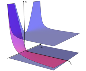
For a given $k_{z}$, we recover the dispersion relation of shallow-water waves with celerity $c=N/|k_{z}|$, see figure 1. The zero-frequency wave band corresponds to geostrophic modes, for which the pressure force balances the Coriolis force. The non-zero frequency bands correspond to hydrostatic, internal inertia–gravity waves. Geostrophic modes and inertia–gravity wave modes are separated by a frequency gap of width $Ro^{-1}$. The existence of this gap is central to the classical derivation of the quasi-geostrophic model.

Figure 1. Dispersion relation of hydrostatic Boussinesq model linearized around a state of rest, adapted from Zeitlin (Reference Zeitlin2018). (a) Unbounded case, $k_{z}$ fixed. There is a frequency gap $\unicode[STIX]{x0394}\unicode[STIX]{x1D714}=f$ between the inertia–gravity wave band and the (flat) geostrophic wave band. (b) Coastal case (wall at $x=0$), $k_{z}$ fixed. The dispersion relation for varying values of $k_{x}$ is projected in ($k_{y},\unicode[STIX]{x1D714}$)-plane. The magenta line corresponds to coastally trapped internal Kelvin waves. (c) Coastal case, $k_{z}>0$. The blue surface at the top represents the bottom boundary of the inertia–gravity wave band. The magenta surface corresponds to the Kelvin-wave dispersion relation. When $k_{z}$ tends to $\infty$ for a given value of $k_{y}$, the Kelvin-wave dispersion relation tends to the flat geostrophic band. This is an obstruction to the classical derivation of quasi-geostrophic equations.

2.3 Unbounded quasi-geostrophic dynamics

The dynamics of geostrophic modes can be decoupled from the dynamics of internal gravity wave modes in the small Rossby number limit $Ro\ll 1$. This amounts to considering a wide frequency gap limit between (slow) geostrophic and (fast) internal inertia–gravity wave modes. The quasi-geostrophic model describes the slow dynamics of the geostrophic mode. It is derived through an asymptotic expansion, with a small parameter given by the Rossby number $Ro\ll 1$, for a fixed Burger number $Bu\sim 1$ (Vallis Reference Vallis2017). This last condition means that typical horizontal flow structures $L$ are of the order of an intrinsic length scale named the Rossby radius of deformation $NH/f$.

2.4 Internal coastal Kelvin waves

The presence of a lateral wall allows for the along-wall propagation of a new class of waves trapped in the across-wall direction, with frequencies filling the frequency gap between inertia–gravity waves and geostrophic modes. Those are the celebrated internal coastal Kelvin waves. Their salient features are derived from the hydrostatic Boussinesq model linearized around a state of rest, in the presence of a lateral (vertical) wall along the $y$-direction. We take the wall at $x=0$ and consider the flow taking place in the region $x>0$, with impermeability boundary condition at the wall: $u(0,y,z,t)=0$. Eigenmodes are of the form $g(x)\text{e}^{\text{i}\unicode[STIX]{x1D714}t-\text{i}k_{y}y-\text{i}k_{z}z}$ with $g(x)$ to be determined. There are two classes of eigenmodes. First, the bulk modes, with $g(x)=\sin (k_{x}x)$ and with the same dispersion relation as in the unbounded case (2.7). Second, an additional branch of boundary modes that correspond to internal coastal Kelvin waves, satisfying geostrophic balance in the along-wall direction with vanishing velocity in the across-wall direction:

(2.8a,b)$$\begin{eqnarray}v=\unicode[STIX]{x2202}_{x}p,\quad \text{with}~\unicode[STIX]{x2202}_{xx}p=-Bu^{-1}\unicode[STIX]{x2202}_{zz}\,p,\quad u=0.\end{eqnarray}$$

Those modes have several features that will play a central role in the derivation of a model coupling interior and boundary dynamics: they are trapped along the wall, unidirectional and propagate as non-rotating hydrostatic internal gravity waves:

(2.9a-c)$$\begin{eqnarray}g(x)=\text{e}^{-x/l},\quad l=\frac{Bu^{1/2}}{|k_{z}|},\quad \unicode[STIX]{x1D714}=-\frac{Bu^{1/2}}{Ro}\frac{k_{y}}{|k_{z}|}.\end{eqnarray}$$

Both the trapping length scale and the phase speed vanish for large vertical wavenumbers.

We readily see on the dispersion relation plotted in figure 1 that the presence of a new branch of Kelvin wave modes filling the frequency gap is an obstruction to the classical derivation of continuously stratified quasi-geostrophic dynamics: whatever the value of the horizontal wavenumber $k_{x}$ and the value of the frequency $\unicode[STIX]{x1D714}$, there is a value of vertical wavenumber $k_{z}$ such that a coastal wave exists. This means that one cannot dismiss the presence of coastal waves when performing the standard multiple- scale expansions leading to quasi-geostrophic dynamics.

Let us consider a Kelvin wave with wavenumber $k_{y}\sim 1$ and frequency $\unicode[STIX]{x1D714}$. Interactions between this wave and geostrophic modes having a typical eddy turnover time $L/U\sim 1$, occurring when $\unicode[STIX]{x1D714}\sim 1$. Substituting this scaling into (2.9), and assuming $Bu\sim 1$, leads to $1/k_{z}\sim Ro$ and $l\sim Ro$ (with dimensions, this gives $1/k_{z}^{\ast }\sim RoH$ and $l^{\ast }\sim RoL$). To conclude, the linear analysis offers important physical insights on possible coupling between the bulk (interior) geostrophic modes and the boundary (coastally trapped) Kelvin waves in the limit of vanishing Rossby numbers, with three properties that will be essential features of the Deremble–Johnson–Dewar model:

1. (i) The interactions involve internal Kelvin waves having a vertical wavelength that scales linearly with the Rossby number, and being confined in a boundary layer with a thickness that also scales linearly with the Rossby numbers.

2. (ii) For all the coastal Kelvin waves, the across-wall velocity $u$ is identically zero. This property will hold at lowest order in the amplitude of the wave for a superposition of coastally trapped modes interacting nonlinearly, since the nonlinear term in the evolution of $u$ is proportional to $u$.

3. (iii) Since there is only one coastally trapped mode for a given value of $(k_{y},k_{z})$, the boundary-layer dynamics that describes the nonlinear evolution of these coastally trapped waves will be governed by a 2-D equation in the $(y,z)$-plane.

3.1 Quasi-geostrophic dynamics in the interior

The interior dynamics is derived from (3.1) to (3.4) following standard procedure based on asymptotic expansion in a low $Ro$ limit (Vallis Reference Vallis2017), with the ansatz

(3.6)$$\begin{eqnarray}[\boldsymbol{u}_{i},p_{i}]=[\boldsymbol{u}_{i,0}^{g},p_{i,0}^{g}]+Ro[\boldsymbol{u}_{i,1}^{g},p_{i,1}^{g}]+O(Ro^{2}).\end{eqnarray}$$

We also assume that typical vertical variations of the pressure fields (up to order 1) between adjacent layers is of order $\unicode[STIX]{x1D6FF}z$, consistent with the assumption of an initial condition satisfying quasi-geostrophic scaling. According to (3.4), interior interface height variations scale linearly with $Ro$.

1. (i) At order 0, one gets geostrophic balance, and hydrostatic balance still holds:

   (3.7a,b)$$\begin{eqnarray}\boldsymbol{u}_{i,0}^{g}=(-\unicode[STIX]{x2202}_{y}\unicode[STIX]{x1D713}_{i},\unicode[STIX]{x2202}_{x}\unicode[STIX]{x1D713}_{i}),\quad \unicode[STIX]{x1D713}_{i}\equiv p_{i,0}^{g},\quad \unicode[STIX]{x1D702}_{i,0}^{g}=-\frac{1}{Bu}\frac{p_{i+1,0}^{g}-2p_{i,0}^{g}+p_{i-1,0}^{g}}{\unicode[STIX]{x1D6FF}z^{2}}.\end{eqnarray}$$

2. (ii) At order 1, we recover quasi-geostrophic dynamics:

   (3.8)$$\begin{eqnarray}\unicode[STIX]{x2202}_{t}q_{i}^{g}+\boldsymbol{u}_{i,0}^{g}\boldsymbol{\cdot }\unicode[STIX]{x1D735}q_{i}^{g}=0,\quad q_{i}^{g}\equiv \unicode[STIX]{x1D6FB}^{2}\unicode[STIX]{x1D713}_{i}+Bu^{-1}(\unicode[STIX]{x1D6FF}z)^{-2}(\unicode[STIX]{x1D713}_{i+1}-2\unicode[STIX]{x1D713}_{i}+\unicode[STIX]{x1D713}_{i}).\end{eqnarray}$$

At this stage, one cannot integrate the dynamics in (3.8) for two reasons, both of them related with potential vorticity inversion: (i) the boundary condition for $\unicode[STIX]{x1D713}$ at the wall remains unknown; (ii) one cannot rule out a source of vorticity within the boundary layer that would affect the streamfunction outside the boundary layer. To address those two issues, it is necessary to examine Kelvin-wave boundary-layer dynamics.

3.2 Kelvin-wave dynamics in the boundary layer

According to the analysis of linearized hydrostatic Boussinesq dynamics in § 2, the Kelvin-wave boundary-layer dynamics is expected to be confined in a region of size $Ro$ away from the wall, with vertical variations of the fields taking place over a distance $Ro$. This motivates the following change of variable:

(3.9a,b)$$\begin{eqnarray}X=\frac{x}{Ro},\quad \unicode[STIX]{x1D6FF}Z=\frac{\unicode[STIX]{x1D6FF}z}{Ro}.\end{eqnarray}$$

The velocity and pressure fields in the boundary layer are decomposed as follows:

(3.10)$$\begin{eqnarray}\displaystyle & v_{i}=v_{i}^{b}(X,y,t)+v_{i,0}^{g}|_{x=0}(y,t)+Rov_{i,1}^{g}|_{x=0}(y,t)+RoX\unicode[STIX]{x2202}_{x}v_{i,0}^{g}|_{x=0}(y,t)+O(Ro^{2}),\qquad & \displaystyle\end{eqnarray}$$

(3.11)$$\begin{eqnarray}\displaystyle & u_{i}=u_{i}^{b}(X,y,t)+u_{i,0}^{g}|_{x=0}(y,t)+Rou_{i,1}^{g}|_{x=0}(y,t)+RoX\unicode[STIX]{x2202}_{x}u_{i,0}^{g}|_{x=0}(y,t)+O(Ro^{2}),\qquad & \displaystyle\end{eqnarray}$$

(3.12)$$\begin{eqnarray}\displaystyle & p_{i}=p_{i}^{b}(X,y,t)+p_{i,0}^{g}|_{x=0}(y,t)+Rop_{i,1}^{g}|_{x=0}(y,t)+RoX\unicode[STIX]{x2202}_{x}p_{i,0}^{g}|_{x=0}(y,t)+O(Ro^{2}).\qquad & \displaystyle\end{eqnarray}$$

The matching condition between inner (index ‘$b$’ for boundary) and outer (index $g$ for interior quasi-geostrophic) solution is

(3.13)$$\begin{eqnarray}\lim _{X\rightarrow +\infty }[u_{i}^{b},v_{i}^{b},p_{i}^{b}]=[0,0,0].\end{eqnarray}$$

The boundary fields are also expanded as

(3.14)$$\begin{eqnarray}[\boldsymbol{u}_{i}^{b},p_{i}^{b}]=[\boldsymbol{u}_{i,0}^{b},p_{i,0}^{b}]+Ro[\boldsymbol{u}_{i,1}^{b},p_{i,1}^{b}]+O(Ro^{2}),\end{eqnarray}$$

and it will be convenient to decompose the total velocity and pressure fields as

(3.15)$$\begin{eqnarray}[\boldsymbol{u}_{i},p_{i}]=[\boldsymbol{u}_{i,0},p_{i,0}]+Ro[\boldsymbol{u}_{i,1},p_{i,1}]+O(Ro^{2}).\end{eqnarray}$$

The fields $[\boldsymbol{u}_{i,0},p_{i,0}]$ and $[\boldsymbol{u}_{i,1},p_{i,1}]$ include the trace of the interior field in the boundary layer regions as defined in (3.10)–(3.12).

Special care must be taken to evaluate the different terms in the expansion of interface height variations $\unicode[STIX]{x1D6FF}\unicode[STIX]{x1D702}_{i}$ defined in (3.4). Indeed, we have assumed that vertical variations of interior pressure between adjacent layers scale as $\unicode[STIX]{x1D6FF}z$, and, based on linear analysis, we anticipated that vertical variations of boundary pressure between adjacent layers scale as $\unicode[STIX]{x1D6FF}Z$. Thus, the interface height variations can be expressed as

(3.16)$$\begin{eqnarray}\unicode[STIX]{x1D6FF}\unicode[STIX]{x1D702}_{i}=\unicode[STIX]{x1D6FF}\unicode[STIX]{x1D702}_{i,0}+O(Ro),\quad \unicode[STIX]{x1D6FF}\unicode[STIX]{x1D702}_{i,0}=-\frac{1}{Bu}\frac{p_{i+1,1}^{b}-2p_{i,1}^{b}+p_{i-1,1}^{b}}{(\unicode[STIX]{x1D6FF}Z)^{2}}.\end{eqnarray}$$

Now that we have introduced the ansatz for the solution in the boundary layer, we write down the rescaled dynamical equations. Momentum equations read

(3.17)$$\begin{eqnarray}\displaystyle & Ro(\unicode[STIX]{x2202}_{t}+Ro^{-1}u_{i}\unicode[STIX]{x2202}_{X}+v_{i}\unicode[STIX]{x2202}_{y})u_{i}=-Ro^{-1}\unicode[STIX]{x2202}_{X}p_{i}+v_{i}, & \displaystyle\end{eqnarray}$$

(3.18)$$\begin{eqnarray}\displaystyle & Ro(\unicode[STIX]{x2202}_{t}+Ro^{-1}u_{i}\unicode[STIX]{x2202}_{X}+v_{i}\unicode[STIX]{x2202}_{y})v_{i}=-\unicode[STIX]{x2202}_{y}p_{i}-u_{i}. & \displaystyle\end{eqnarray}$$

It will be convenient to use potential vorticity as a third dynamical equation:

(3.19)$$\begin{eqnarray}(\unicode[STIX]{x2202}_{t}+Ro^{-1}u_{i}\unicode[STIX]{x2202}_{X}+v_{i}\unicode[STIX]{x2202}_{y})q_{i}=0,\quad q_{i}=\frac{1+\unicode[STIX]{x1D701}_{i}}{1+\unicode[STIX]{x1D6FF}\unicode[STIX]{x1D702}_{i}},\,\unicode[STIX]{x1D701}_{i}\equiv \unicode[STIX]{x2202}_{X}v_{i}-Ro\unicode[STIX]{x2202}_{y}u_{i}.\end{eqnarray}$$

Consistent with the assumption of an initial condition satisfying quasi-geostrophic scaling, material conservation of potential vorticity for a fluid particle with initial relative vorticity $\unicode[STIX]{x1D701}_{i}^{(t=0)}\sim Ro$ and initial interface thickness variation $\unicode[STIX]{x1D6FF}\unicode[STIX]{x1D702}_{i}^{(t=0)}\sim Ro$ can be recast as

(3.20)$$\begin{eqnarray}\unicode[STIX]{x1D701}_{i}-\unicode[STIX]{x1D6FF}\unicode[STIX]{x1D702}_{i}=O(Ro).\end{eqnarray}$$

We substitute the ansatz (3.10)–(3.12), (3.6), (3.14) in the rescaled dynamical system (3.17), (3.18), (3.20) and collect terms at each order with respect to $Ro$.

1. (i) At order $-1$, the momentum equation in $X$-direction yields

   (3.21)$$\begin{eqnarray}\unicode[STIX]{x2202}_{X}p_{i,0}=0.\end{eqnarray}$$

2. (ii) At order 0, the momentum and potential vorticity equations yield, respectively,

   (3.22)$$\begin{eqnarray}\displaystyle & u_{i,0}\unicode[STIX]{x2202}_{X}u_{i,0}=-\unicode[STIX]{x2202}_{X}p_{i,1}+v_{i,0}, & \displaystyle\end{eqnarray}$$
   (3.23)$$\begin{eqnarray}\displaystyle & u_{i,0}\unicode[STIX]{x2202}_{X}v_{i,0}=-\unicode[STIX]{x2202}_{y}p_{i,0}-u_{i,0}, & \displaystyle\end{eqnarray}$$
   (3.24)$$\begin{eqnarray}\displaystyle & \unicode[STIX]{x2202}_{X}v_{i,0}-\unicode[STIX]{x1D6FF}\unicode[STIX]{x1D702}_{i,0}=0. & \displaystyle\end{eqnarray}$$
   Differentiating (3.23) by $X$ and using (3.21) leads to $\unicode[STIX]{x2202}_{X}(u_{i,0}(\unicode[STIX]{x2202}_{X}v_{i,0}+1))=0$. Using the impermeability condition (3.5) leads then to $u_{i,0}(\unicode[STIX]{x2202}_{X}v_{i,0}+1)=0$ for all $X$. The case $\unicode[STIX]{x2202}_{X}v_{i}=-1$ corresponds to a vanishing interface thickness, i.e. $1+\unicode[STIX]{x1D6FF}\unicode[STIX]{x1D702}_{i,0}=0$, according to (3.24). This may occur along shock lines. From now on, we describe the flow dynamics away from these singularities. This corresponds to the second case, $u_{i,0}(X,y,t)=0$. Using the matching condition (3.13), we find an impermeability condition for the geostrophic (interior) velocity field, and a vanishing across-wall velocity in the boundary layer:
   (3.25a,b)$$\begin{eqnarray}u_{i,0}^{g}|_{x=0}=0,\quad u_{i,0}^{b}(X,y,t)=0.\end{eqnarray}$$
   Equation (3.23) is now further simplified as $\unicode[STIX]{x2202}_{y}p_{i,0}=0$. Using this equation together with (3.21) and the matching condition (3.13) yields
   (3.26a,b)$$\begin{eqnarray}p_{i,0}^{b}=0,\quad p_{i,0}^{g}|_{x=0}(y,t)=\unicode[STIX]{x1D713}_{i,wall}(t).\end{eqnarray}$$
   The second equality is the standard impermeability condition for quasi-geostrophic flows along a wall. The value of $\unicode[STIX]{x1D713}_{i,wall}$ will be determined using layerwise global mass conservation later on. Finally, equations (3.22) and (3.24) simplify to
   (3.27a,b)$$\begin{eqnarray}v_{i,0}^{b}=\unicode[STIX]{x2202}_{X}p_{i,1}^{b},\quad \frac{\unicode[STIX]{x2202}^{2}}{\unicode[STIX]{x2202}X^{2}}p_{i,1}^{b}=-\frac{1}{Bu}\frac{p_{i+1,1}^{b}-2p_{i,1}^{b}+p_{i-1,1}^{b}}{(\unicode[STIX]{x1D6FF}Z)^{2}}.\end{eqnarray}$$
   This shows that the triplet of boundary-layer fields $[\boldsymbol{u}_{i,0}^{b},p_{i,0}^{b}]$ satisfies the polarization relation of coastal Kelvin waves, as in (2.8). The boundary fields are then fully prescribed by the amplitude of $v_{i}^{b}$ at the boundary $X=0$. Their dynamics is obtained at next order.

3. (iii) At order 1, the momentum equation in the $y$-direction evaluated at the wall yields

   (3.28)$$\begin{eqnarray}\text{at}~X=0:\unicode[STIX]{x2202}_{t}v_{i,0}+\unicode[STIX]{x2202}_{y}\left({\textstyle \frac{1}{2}}v_{i,0}^{2}+p_{i,1}\right)=0.\end{eqnarray}$$
   We have used $u_{i}(0,y,t)=0$ and the order-1 impermeability constraint. Equation (3.28) can be recast as a dynamical evolution for $v_{i,0}^{b}(0,y,t)=v_{i,0}(0,y,t)-v_{i,0}^{g}(0,y,t)$, assuming that geostrophic fields are known. Noticing that $\unicode[STIX]{x2202}_{y}p_{i,1}|_{X=0}=\unicode[STIX]{x2202}_{y}p_{i,1}^{b}|_{X=0}(y,t)$, the combination of (3.27) with (3.28) and boundary condition (3.13) provides the system of equations derived in Deremble et al. (Reference Deremble, Johnson and Dewar2017).

3.3 Potential vorticity production by shallow-water shocks

Dewar & Hogg (Reference Dewar and Hogg2010), Hogg et al. (Reference Hogg, Dewar, Berloff and Ward2011) and Deremble et al. (Reference Deremble, Johnson and Dewar2017) showed that the boundary-layer dynamics leads to shocks and the concomitant creation of cyclonic vorticity. Based on global conservation of circulation, Deremble et al. (Reference Deremble, Johnson and Dewar2017) proposed a model for the feedback of these shocks on the interior quasi-geostrophic dynamics. We propose here a more local justification of their model, relying on the theory of rotating shallow-water shocks (Peregrine Reference Peregrine1998; Pratt & Whitehead Reference Pratt and Whitehead2007; Zeitlin Reference Zeitlin2018).

A shallow-water shock line, in the $X$-direction indexed by $s$ in layer $i$ and located at $y=y_{s,i}(t)$ is associated with a jump of the Bernoulli potential across the shock, see e.g. Zeitlin (Reference Zeitlin2018):

(3.29)$$\begin{eqnarray}[B_{i}]\equiv B_{i}(X,y_{s,i}^{+})-B_{i}(X,y_{s,i}^{-}),\quad B_{i}(X,y_{s,i}^{\pm })\equiv \frac{\boldsymbol{u}_{i}^{2}(X,y_{s,i}^{\pm })}{2}+p_{i}(X,y_{s,i}^{\pm }).\end{eqnarray}$$

When the value of $[B_{i}]$ varies along the shock, in the $X$-direction, there is a jump of potential vorticity across the shock (Zeitlin Reference Zeitlin2018):

(3.30)$$\begin{eqnarray}[q_{i}]\equiv q_{i}(X,y_{s,i}^{+})-q_{i}(X,y_{s,i}^{-})=Ro^{-1}\frac{\unicode[STIX]{x2202}_{X}([B_{i}]-{\dot{y}}_{s,i}[v_{i}])}{h_{i}(v_{i}-{\dot{y}}_{s,i})},\end{eqnarray}$$

where $[v_{i}]=v_{i}(X,y_{s,i}^{+},t)-v_{i}(X,y_{s,i}^{-},t)$ is the velocity jump across the shock, ${\dot{y}}_{s,i}\equiv \text{d}y_{s,i}/\text{d}t$ is the shock velocity and $h_{i}(v_{i}-{\dot{y}}_{s,i})$ is the mass flux through the shock for an observer moving with the shock. This mass flux is conserved across the shock, with $[h_{i}(v_{i}-{\dot{y}}_{s,i})]=0$. The combination of a potential vorticity jump and a constant mass flux through the shock implies a net production of potential vorticity per unit time and per unit shock length, see e.g. Zeitlin (Reference Zeitlin2018). The total amount of potential vorticity production at $y=y_{s,i}$ in the boundary-layer region is thus

(3.31)$$\begin{eqnarray}\int _{0}^{+\infty }\,\text{d}X\unicode[STIX]{x2202}_{X}([B_{i}]-{\dot{y}}_{s,i}[v_{i}])={\dot{y}}_{s,i}[v_{i}]_{X=0}-[B_{i}]_{X=0},\end{eqnarray}$$

where the right-hand side is evaluated at $(X=0,y=y_{s,i})$. We have used the fact that there is no shock in the (quasi-geostrophic) interior, for $X\rightarrow +\infty$.

The net production of potential vorticity in the boundary layer contradicts our assumption of materially conserved potential vorticity used to derive the Kelvin-wave dynamics in the boundary layer. One way to have a self-consistent model taking into account the local inviscid production of vorticity at $y=y_{s,i}$ is to substitute in (3.8) the total amount of potential vorticity of (3.31), at a distance $x=\sqrt{Ro}$ much greater than the boundary layer of size $Ro$, while remaining asymptotically close to the wall:

(3.32)$$\begin{eqnarray}\unicode[STIX]{x2202}_{t}q_{i}^{g}+\boldsymbol{u}_{i}^{g}\boldsymbol{\cdot }\unicode[STIX]{x1D735}q_{i}^{g}=\unicode[STIX]{x1D6FF}(x-\sqrt{Ro})\unicode[STIX]{x1D6FF}(y-y_{s,i})({\dot{y}}_{s,i}[v_{i}]_{X=0}-[B_{i}]_{X=0}).\end{eqnarray}$$

This infinitesimal shift of potential vorticity production from the boundary layer to the interior region is the only phenomenological step of the model derivation. It is motivated by numerical simulations showing production of cyclones through the detachment of boundary layers close to the shock location in primitive equation models (Deremble et al. Reference Deremble, Johnson and Dewar2017). This can also be interpreted as the continuous version of the discrete numerical algorithm used by Deremble et al. (Reference Deremble, Johnson and Dewar2017) to simulate their coupled reduced model: for a given grid size, the location of the source term at $x=\sqrt{Ro}$ guarantees that potential vorticity injection occurs within the cell adjacent to the wall in the limit $Ro\rightarrow 0$.

To be consistent with this procedure of potential vorticity injection in the interior following the formation of shocks in the boundary, the total circulation in the boundary regions must be left invariant, which, assuming that it is initially zero, implies

(3.33)$$\begin{eqnarray}\unicode[STIX]{x1D6E4}_{i}=\unicode[STIX]{x1D6E4}_{i}^{g},\quad \text{with}~\unicode[STIX]{x1D6E4}_{i}\equiv -\int _{-\infty }^{+\infty }\,\text{d}yv_{i,0},\,\unicode[STIX]{x1D6E4}_{i}^{g}\equiv -\int _{-\infty }^{+\infty }\,\text{d}yv_{i,0}^{g}.\end{eqnarray}$$

3.4 Mass conservation, quasi-geostrophic circulation and final set of equations

The full dynamical system coupling boundary dynamics with quasi-geostrophic interior is yet not closed, as one still must determine the value of $\unicode[STIX]{x1D713}_{i,wall}$ introduced in (3.26). This is settled by using layerwise global mass conservation:

(3.34)$$\begin{eqnarray}\langle \unicode[STIX]{x1D6FF}\unicode[STIX]{x1D702}_{i}\rangle =0,\quad \text{with}~\langle \unicode[STIX]{x1D6FF}\unicode[STIX]{x1D702}_{i}\rangle \equiv \int _{0}^{+\infty }\,\text{d}x\int _{-\infty }^{+\infty }\,\text{d}y\unicode[STIX]{x1D6FF}\unicode[STIX]{x1D702}_{i}.\end{eqnarray}$$

The difficulty with respect to classical quasi-geostrophic models is that variations of mass in the boundary layers are of the same order as variations of mass in the interior. Despite this subtlety, the use of (3.33) allows us to recover the constraint (see appendix B):

(3.35)$$\begin{eqnarray}\langle \unicode[STIX]{x1D713}_{i+1}+\unicode[STIX]{x1D713}_{i-1}-2\unicode[STIX]{x1D713}_{i}\rangle =0.\end{eqnarray}$$

The set of boundary values $\unicode[STIX]{x1D713}_{i,wall}$ is deduced from the set of constraints in (3.35), following standard procedure (McWilliams Reference McWilliams1977). Let us note that (3.35) implies instantaneous adjustment of the mass in each interior layer. The reason is that we assumed previously that quasi-geostrophic motion has typical vertical scale of order 1 (size $H$ in dimensional units), and that Kelvin waves associated with vertical variations of order 1 are filtered out in the asymptotic expansion. Note that our phenomenological procedure of potential vorticity injection is such that structures of vertical size much smaller than $H$ can be formed in the interior, depending on shock properties in the boundary layer. This injection procedure induces, therefore, an inconsistency with respect to the initial hypothesis on the size of interior flows. By applying mass conservation (3.35), we continue to assume instantaneous adjustment for those smaller scale structures in the interior. Possible resonances between slow Kelvin-wave dynamics and interior quasi-geostrophic flow are still taken into account through the boundary-layer equation (3.28).

Finally, the full coupled system is given by potential vorticity advection in (3.32) and Kelvin-wave dynamics in (3.28). The interior velocity field is obtained by inversion of the quasi-geostrophic potential vorticity field defined in (3.8), using the lateral boundary conditions in (3.26) and the constraints of (3.35). Kelvin-wave dynamics in (3.28) depends on the geostrophic interior field evaluated at the boundary; in turn, equation (3.28) is used to find shock locations and evaluate the corresponding velocity and Bernoulli potential jumps appearing in the right-hand side of (3.32), and defined in (3.29). Thus, the knowledge of potential vorticity production is bound to the knowledge of Bernoulli potential jumps across shocks in the boundary-layer dynamics. We have until now not explained how to determine the actual value of such Bernoulli potential jumps. In the case of a one-layer shallow-water model, one just needs to apply standard local mass and momentum conservation across the shock. However, the problem is indeterminate in the case of multiple-layer shallow-water flows, and no universal rule exists (Zeitlin Reference Zeitlin2018). One then needs either to introduce additional phenomenological assumptions on the shock behaviour, or to bypass this issue by regularizing the boundary Kelvin-wave dynamics with dissipative terms. In the latter case, the Bernoulli potential jumps are estimated numerically across quasi-shocks that are defined at locations where gradients exceed a given threshold; this is the approach followed in Deremble et al. (Reference Deremble, Johnson and Dewar2017), who introduced viscous dissipation in (3.28).

3.5 Conservation of quasi-geostrophic energy

Let us now consider the case of a finite-depth ocean with $N$ layers of thickness $h$, such that $Nh=1$, with a rigid lid approximation (at layer $i=N$) and flat bottom boundary condition (at layer $i=1$). The dynamics is the same as in the case of an infinite number of layers, with two additional constraints related to upper and lower boundary conditions, namely $\unicode[STIX]{x1D713}_{N+1}=\unicode[STIX]{x1D713}_{N}$ and $\unicode[STIX]{x1D713}_{0}=\unicode[STIX]{x1D713}_{1}$, respectively. The quasi-geostrophic energy is defined as

(3.36)$$\begin{eqnarray}E^{g}\equiv \frac{h}{2}\mathop{\sum }_{i=1}^{N}\left\langle (\unicode[STIX]{x1D735}\unicode[STIX]{x1D713}_{i})^{2}+\frac{1}{Bu}\left(\frac{\unicode[STIX]{x1D713}_{i}-\unicode[STIX]{x1D713}_{i-1}}{\unicode[STIX]{x1D6FF}z}\right)^{2}\right\rangle .\end{eqnarray}$$

We assume the presence of $n_{i}$ shocks in each layer $i$. The shocks are indexed by $(s,i)$ with $1\leqslant s\leqslant n_{i}$. Their location in the $y$-direction is denoted $y_{s,i}(t)$, and the corresponding potential vorticity injection rate is $\unicode[STIX]{x1D6FE}_{s,i}\equiv {\dot{y}}_{s,i}[v_{i}]-[B_{i}]$, see (3.32). The temporal evolution of quasi-geostrophic energy is computed by using the dynamical equation (3.32), the definition of quasi-geostrophic potential vorticity in (3.8), as well as the definition of circulation in (3.33) and mass conservation in (3.35):

(3.37a,b)$$\begin{eqnarray}\frac{\text{d}}{\text{d}t}E^{g}=h\mathop{\sum }_{i=1}^{N}\left(-\unicode[STIX]{x1D713}_{i,wall}\frac{\text{d}\unicode[STIX]{x1D6E4}_{i}^{g}}{\text{d}t}+\mathop{\sum }_{s=1}^{n_{i}}\unicode[STIX]{x1D6FE}_{s,i}\unicode[STIX]{x1D713}_{i}(\sqrt{Ro},y_{s,i},t)\right),\quad \frac{\text{d}}{\text{d}t}\unicode[STIX]{x1D6E4}_{i}^{g}=\mathop{\sum }_{s=1}^{n_{i}}\unicode[STIX]{x1D6FE}_{s,i}.\end{eqnarray}$$

Following the conventions used for the asymptotic analysis, the initial energy and the initial circulations are of order 1; according to this asymptotic analysis, the potential vorticity injection rate $\unicode[STIX]{x1D6FE}_{s,i}$ is also of order 1. Using $hN\sim 1$ and $\unicode[STIX]{x1D713}_{i}(\sqrt{Ro},y_{s,i})=\unicode[STIX]{x1D713}_{i,wall}+\sqrt{Ro}\unicode[STIX]{x2202}_{x}\unicode[STIX]{x1D713}|_{0,y_{s,i}}+o(\sqrt{Ro})$, we find that the total quasi-geostrophic energy vanishes in the limit $Ro\rightarrow 0$. We conclude that quasi-geostrophic energy is conserved, unless the asymptotic approach fails in such a way that $\unicode[STIX]{x1D6FE}_{s,i}$ scales as $1/\sqrt{Ro}$. This result does not contradict the observation of enhanced dissipation in the presence of a coast (Deremble et al. Reference Deremble, Johnson and Dewar2017); it just suggests that the amplitude of enhanced dissipation should tend to zero with $Ro$, so that the corresponding energy sink in the actual ocean would be a finite-$Ro$ effect. It will be interesting to investigate how enhanced dissipation actually scales with $Ro$ in numerical models.