1. INTRODUCTION
The inertial navigation system (INS) is a very common navigation systems. An INS can output comprehensive navigation information, such as attitude, velocity and position (Xiong et al., Reference Xiong, Liu, Lai and Jiang2011). The main component of an INS is the inertial measurement unit (IMU) (Lai et al., Reference Lai, Lv, Liu and Jiang2012a), which consists of gyros and accelerometers and supplies angular velocity and acceleration information. Since INS is a dead-reckoning system, the position, velocity and attitude errors produced by gyros' errors and accelerometers' errors spread over time (Lai et al., Reference Lai, Xiong, Liu and Jiang2012b).
The rotation technique is an effective method to improve an INS's accuracy, and INS with the rotation technique is called a rotational inertial navigation system (RINS) (Ishibashi et al., Reference Ishibashi, Aoki, Yamamoto and Tsukioka2006). In a RINS, the IMU is mounted on a rotary table, which rotates the IMU back and forth to modulate the errors of gyros and accelerometers, so as to reduce the navigation errors (Yang and Miao, Reference Yang and Miao2004; Qian et al., Reference Qian, Liu, Zhao and Zhu2009). RINSs are widely used in marine navigation, in systems such as the AN/WSN-7B (Tucker and Levinson, Reference Tucker and Levinson2000) and Mk 49 (Levinson et al., Reference Levinson, Horst and Willcocks1994). They can supply accurate navigation information for several days. Recently, the rotation technique has also been used in north-finding systems with Micro-electromechanical Systems (MEMS) gyros (Iozan et al., Reference Iozan, Kirkko-Jaakkola, Collin, Takala and Rusu2012; Prikhodko et al., Reference Prikhodko, Zotov, Trusov and Shkel2011).
The rotation scheme directly affects the navigation accuracy of the RINS (Yuan et al., Reference Yuan, Liao and Han2012). When designing a rotation scheme, there are two main principles to be followed: one is to reduce the inherent errors of the IMU; the other is to prevent new errors brought by the rotation. Therefore, in order to design a good rotation scheme, it is important to know the compensation effects of all the IMU's errors.
The IMU errors mainly consist of two parts, the deterministic and the stochastic (El-Diasty and Pagiatakis, Reference El-Diasty and Pagiatakis2008). According to current research, the compensation effects of the deterministic errors are clear (Ben et al., Reference Ben, Chai, Gao and Sun2010), but the compensation effects of the stochastic errors are as yet unknown. In this paper, the compensation effects of gyros' stochastic errors in a RINS are analysed and the quantitative formulae are given. Actually, as a basic research on the RINS, the analysis of this paper does not only give a reference to the design of the rotation scheme, but also contributes to the error analysis and the optimization study of the RINS (Dushman, Reference Dushman1962; Poor, Reference Poor1992).
In order to achieve the goal, the propagation characteristics of gyros' stochastic errors both in an INS and in a RINS are needed. Hammon (Reference Hammon1960; Reference Hammon1962) derived the propagation formulae of gyros' stochastic errors in an INS. The INS model he used is simplified for short-term navigation. However, RINSs are usually used for long-term navigation. So the propagation characteristics of gyros' stochastic errors in a long-term working INS and a long-term working RINS need to be analysed. Then the compensation effects of gyros' stochastic errors brought by the rotation technique can be obtained by comparing the propagation characteristics in an INS and a RINS. In this study, two points need to be stated:
1) The stochastic errors of gyros are modelled as Gaussian white (GW) noise and as a first-order Markov process. The GW noise is used to express the high frequency component of the stochastic errors, while the first-order Markov process is for the low frequency component.
2) For a RINS the position accuracy is most concerned, so the propagation characteristics of a gyros' stochastic errors are analysed only for the longitude and latitude results.
In the subsequent sections, we first introduce the method used for analysing the stochastic error propagation characteristics in an INS. Then the INS's and the RINS's position error equations response to gyros' stochastic errors are derived respectively in Sections 3 and 4. At the end, numerous simulations are devised to verify the proposed theory.
2. METHODOLOGY
Since the INS's error response to gyros' stochastic errors can be assumed to be a linear system, the impulse response method is adopted. Assuming f(t) is the impulse response function of the INS, R g(t 1,t 2) is the autocorrelation function of gyros' stochastic errors, e(t) is the navigation error produced by gyros' stochastic errors. According to the theory of the impulse response method, the autocorrelation function of the navigation error can be derived as:
 $$R_n (t_1, t_2 ) = E[e(t_1 )e(t_2 )] = \int_0^{t_2} {\int_0^{t_1} {\,f\,(\tau _1 )}} f\,(\tau _2 )R_g (t_1 - \tau _1, t_2 - \tau _2 )d\tau _1 d\tau _2 $$
where E[] is an averaging operator, t 1,t 2 are time variables, τ 1,τ 2 are integral variables. Then the variance of the navigation error can be derived as:
 $$R_n (t,t) = \int_0^t {\int_0^t {\,f\,(\tau _1 )}} f\,(\tau _2 )R_g (t - \tau _1, t - \tau _2 )d\tau _1 d\tau _2 $$
From Equation (2), it can be seen that the navigation error can be evaluated after acquiring the autocorrelation function of gyros' stochastic errors and the impulse response function of the INS.
2.1. The Autocorrelation Function of a Gyro's Stochastic Errors
The models of Fibre Optic Gyros' (FOGs') stochastic errors are complex and generally not unique (IEEE standard, 1998; Flenniken et al., Reference Flenniken, Wall and Bevly2005), but some typical models are usually used. A simple model is assumed to consist of GW noise and first-order Markov process. In discrete time, the model can be expressed as (El-Diasty and Pagiatakis, Reference El-Diasty and Pagiatakis2008):
 $$g_k = w_k + m_k $$
where g k is a gyro's discrete stochastic error, w k is the discrete GW noise with the standard deviation (SD) denoted as q w and m k is the discrete first order Markov process with the expression as:
 $$m_k = e^{ - \Delta T/T_m} m_{k - 1} + wm_k $$
where ΔT is the sample time, T m is the correlation time, and wm k is a zero-mean discrete GW noise with the SD denoted as q mw and called the driving GW noise.
The autocorrelation function of the GW noise can be written as:
 $$R_w (t_1, t_2 ) = q_w ^2 \Delta T \cdot \delta (t_1 - t_2 )$$
where δ(x) is the unit impulse function.
The autocorrelation function of the first-order Markov process can be written as:
 $$R_m (t_1, t_2 ) = \sigma _r ^2 e^{ - \left| {t_2 - t_1} \right|/T_m} $$
where  $\sigma _r ^2 = q_{mw} ^2 /(2\Delta T/T_m )$.
2.2. The Impulse Response Function of the INS
Usually there are three gyros in an INS. In this section, the impulse response functions between the position error and each gyro's error are derived.
In this paper, the coordinate systems are defined as follows: the inertial coordinate system is the reference coordinate for the inertial components and denoted by i; the navigation coordinate system is chosen as the local East-North-Up (ENU) coordinate and denoted by n; the body coordinate system is vehicle-carried and denoted by b. The error state equation of the INS under the stationary state can be written as (Groves, Reference Groves2013):
 $$\hskip-44pt\eqalign{\left( {\matrix{ {\dot \psi _E} \cr {\dot \psi _N} \cr {\dot \psi _U} \cr {\delta \dot v_E} \cr {\delta \dot v_N} \cr {\delta \dot L} \cr {\delta \dot \lambda} \cr}} \right) =\tab \left( {\matrix{ 0 & {\omega _{ie} \sin L} & { - \omega _{ie} \cos L} & 0 & { - 1/R} & 0 & 0 \cr { - \omega _{ie} \sin L} & 0 & 0 & {1/R} & 0 & { - \omega _{ie} \sin L} & 0 \cr {\omega _{ie} \cos L} & 0 & 0 & {\tan L/R} & 0 & {\omega _{ie} \cos L} & 0 \cr 0 & { - g} & 0 & 0 & {2\omega _{ie} \sin L} & 0 & 0 \cr g & 0 & 0 & { - 2\omega _{ie} \sin L} & 0 & 0 & 0 \cr 0 & 0 & 0 & 0 & {1/R} & 0 & 0 \cr 0 & 0 & 0 & {1/R\cos L} & 0 & 0 & 0 \cr}} \right)\hskip-42pt\cr\tab\times\left( {\matrix{ {\psi _E} \cr {\psi _N} \cr {\psi _U} \cr {\delta v_E} \cr {\delta v_N} \cr {\delta L} \cr {\delta \lambda} \cr}} \right) + \left( {\matrix{ {\varepsilon _x} \cr {\varepsilon _y} \cr {\varepsilon _z} \cr 0 \cr 0 \cr 0 \cr 0 \cr}} \right)$$
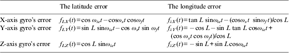
where [ψ E ψ N ψ U] represents the platform error angle projected on the n-frame, [δv E δv N] represents the east velocity error and the north velocity error, [δL δλ] represents the latitude error and the longitude error, [ε x ε y ε z] represents gyros' errors projected on the n-frame, ω ie is the Earth's rotation angular velocity, L is the local latitude, R is the earth radius, g is the acceleration of gravity. Since the analysis is for the stationary state, the b-frame is assumed to be coincident with the n-frame, then [ε x ε y ε z] equals to three gyros' errors. The impulse response functions can be solved from Equation (7), and the specific derived formulae are shown in Table 1.
In Table 1, ω s equals to g/R and is called the Schuler angular frequency, ω f equals ω ie sinL and is called the Foucault angular frequency. The subscript of f LX(t) means that the impulse response function is between the latitude error and X-axis gyro's error. It can be found from Table 1 that f LX(t), f λ X(t), f LY(t), f LZ(t) only consist of sinusoidal components, and f λ Y(t), f λ Z(t) consist of sinusoidal components and constant components.
3. STOCHASTIC ERROR PROPAGATION IN A LONG-TERM WORKING INS
In this section, the error propagation formulae of the GW noise and the first-order Markov process in an INS are derived and simplified for long-term navigation. As mentioned, only the position errors are considered.
3.1. The GW Noise Error Propagation Formulae
According to the analysis in Section 2, the position errors response to gyros' GW noises can be solved by plugging the autocorrelation function of the GW noise (shown as Equation (5)) and the impulse response functions (shown in Table 1) into Equation (2). In the following, the longitude errors and the latitude errors response to three gyros' GW noises will be derived separately.
The variance of the longitude error response to the X-axis gyro's GW noise can be expressed as:
 $$\eqalign{e_{\lambda X}^{sw} (t)^2 = & \int_0^t {\int_0^t {\,f_{\lambda X} (\tau _1 )}} f_{\lambda X} (\tau _2 )R_w (t - \tau _1, t - \tau _2 )d\tau _1 d\tau _2 \cr = & \int_0^t {\int_0^t {\,f_{\lambda X} (\tau _1 )}} f_{\lambda X} (\tau _2 )q_w ^2 \Delta T\delta (\tau _1 - \tau _2 )d\tau _1 d\tau _2 \cr = &\, q_w ^2 \Delta T\int_0^t {\,f_{\lambda X} (\tau _1 )^2 d\tau _1}} $$
where the subscript of e λXsw stands for the longitude error response to the X-axis gyro's error, the superscript means that the error source is the gyro's GW noise and the analysis is for a “stationary” INS instead of a RINS.
Plugging the expression of f λ X (τ 1) from Table 1 into Equation (8), the expression of e λXsw(t)2 can be derived. Due to the complex integration computation, the derived complete expression of e λXsw(t)2 includes more than 100 sinusoidal items, which is too long to be listed, so the expression of e λXsw(t)2 needs to be simplified. When the formula is for long-term navigation, some items can be omitted and the expression of e λXsw(t) can be simplified as follows:
 $$\eqalign{e_{\lambda X}^{sw} (t) \approx 0 {\cdot} 5q_w \tan L\sqrt {\Delta T[2t + t/\sin ^2 L - \sin (2\omega _{ie} t)/\omega _{ie} - \sin (2\omega _f t)/(2\omega _f \sin ^2 L)]} $$
Since e λXsw(t) is the standard deviation of the longitude error, it equals to the root mean square error (RMSE) of longitude. Using the same approach, the RMSE of the latitude response to the X-axis gyro's GW noise can be derived as follows:
 $$e_{LX}^{sw} (t) \approx q_w \sqrt {\Delta T[3t/4 + \sin (2\omega _f t)/(8\omega _f ) + \sin (2\omega _{ie} t)/(4\omega _{ie} )]} $$
Table 1. The impulse response functions between the position error and three gyros' errors.

The RMSE of the longitude response to the Y-axis gyro's GW noise can be derived as follows:
 $$e_{\lambda Y}^{sw} (t)\! \approx\! q_w \sqrt {\Delta T[\sin (2\omega _f t)/(8\cos ^2 L\omega _f ) + t\cos ^2 L \hskip-1pt+\hskip-1pt t\tan ^2 L/2 \hskip-1pt+\hskip-1pt t\cos ^2 L/4 \!-\! t\sin ^2 L/2]} $$
The RMSE of the latitude response to the Y-axis gyro's GW noise can be derived as follows:
 $$\eqalign{e_{LY}^{sw} (t) \approx 0 \cdot 5q_w \sin L\sqrt {\Delta T[2t + t/\sin ^2 L - \sin (2\omega _{ie} t)/\omega _{ie} - \sin (2\omega _f t)/(2\omega _f \sin ^2 L)]} $$
The RMSE of the longitude response to the Z-axis gyro's GW noise can be derived as follows:
 $$e_{\lambda Z}^{sw} (t) \approx q_w \sin L\sqrt {\Delta T[3\omega _{ie} t - 4\sin (\omega _{ie} t) + \sin (2\omega _{ie} t)/2]/(2\omega _{ie} )} $$
The RMSE of the latitude response to the Z-axis gyro's GW noise can be derived as follows:
 $$e_{LZ}^{sw} (t) \approx q_w \cos L\sqrt {\Delta T[\omega _{ie} t - \sin (2\omega _{ie} t)/2]/(2\omega _{ie} )} $$
 Through Equations (9) to (14), it can be seen that the RMSE of the latitude and the longitude increases proportional to  $q_w \sqrt {\Delta T} $ and approximately proportional to
  $\sqrt t $.
3.2. The Error Propagation Formulae of the First-order Markov Process
According to the autocorrelation function of the first-order Markov process (shown as Equation (6)), the variance of the longitude error response to the X-axis gyro's first-order Markov process can be expressed as:
 $$\eqalign{e_{\lambda X}^{sm} (t)^2 & = \int_0^t {\int_0^t {\,f_{\lambda X} (\tau _1 )}} f_{\lambda X} (\tau _2 )R_m (t - \tau _1, t - \tau _2 )d\tau _1 d\tau _2 \cr & = \int_0^t {\int_0^t {\,f_{\lambda X} (\tau _1 )}} f_{\lambda X} (\tau _2 )\sigma _r ^2 e^{ - \left| {\tau _2 - \tau _1} \right|/T_m} d\tau _1 d\tau _2} $$
where the superscript of e λXsm means that the error source is the gyro's first-order Markov process and the analysis is for an INS. In Equation (15), since τ 1 and τ 2 are the integral variables, during the equation simplification both conditions including τ 2⩾τ 1 and τ 1⩾τ 2 need to be considered. When τ 2⩾τ 1, Equation (15) transforms to:
 $$\eqalign{e_{\lambda X}^{sm} (t)^2 & = \int_0^t {\int_0^{\tau _2} {\,f_{\lambda X} (\tau _1 )}} f_{\lambda X} (\tau _2 )\sigma _r ^2 e^{ - (\tau _2 - \tau _1 )/T_m} d\tau _1 d\tau _2 \;\;\;\;(\tau _2 \geqslant \tau _1 ) \cr & = \sigma _r ^2 \int_0^t {\int_0^{\tau _2} {\,f_{\lambda X} (\tau _1 )}} e^{\tau _1 /T_m} d\tau _1 f_{\lambda X} (\tau _2 )e^{ - \tau _2 /T_m} d\tau _2 \;\;(\tau _2 \geqslant \tau _1 )} $$
When τ 1⩾τ 2,Equation (15) transforms to:
 $$\eqalign{e_{\lambda X}^{sm} (t)^2 & = \int_0^t {\int_0^{\tau _1} {\,f_{\lambda X} (\tau _1 )}} f_{\lambda X} (\tau _2 )\sigma _r ^2 e^{ - (\tau _1 - \tau _2 )/T_m} d\tau _2 d\tau _1 \;\;\;\;(\tau _1 \geqslant \tau _2 ) \cr & = \sigma _r ^2 \int_0^t {\int_0^{\tau _1} {\,f_{\lambda X} (\tau _2 )}} e^{\tau _2 /T_m} d\tau _2 f_{\lambda X} (\tau _1 )e^{ - \tau _1 /T_m} d\tau _1 \;\;(\tau _1 \geqslant \tau _2 )} $$
Combining the simplification results under the condition τ 2⩾τ 1 and the condition τ 1⩾τ 2, Equation (15) transforms to:
 $$e_{\lambda X}^{sm} (t)^2 = 2\sigma _r ^2 \int_0^t {\int_0^{\tau _2} {\,f_{\lambda X} (\tau _1 )}} e^{\tau _1 /T_m} d\tau _1 f_{\lambda X} (\tau _2 )e^{ - \tau _2 /T_m} d\tau _2 $$
After plugging f λ X(t) (shown in Table 1) into Equation (18), the simplified result for long-term navigation is as follows:
 $$e_{\lambda X}^{sm} (t) \approx\, \displaystyle{{\sigma _r T_m \omega _s \sqrt {T_m (1 + \sin ^2 L + \omega _s ^2 T_m ^2 \sin ^2 L)t}} \over {(1 + \omega _{ie} ^2 T_m ^2 )(1 + \omega _s ^2 T_m ^2 )\cos L}}$$
Using the same approach, the RMSE of the latitude response to the X-axis gyro's first-order Markov process can be derived as follows:
 $$e_{LX}^{sm} (t) \approx \displaystyle{{\sigma _r T_m ^2 \omega _s \sqrt {T_m [3t/T_m ^2 + \omega _s ^2 t + T_m ^2 \omega _s ^2 \omega _{ie} ^2 t + \omega _s ^2 \sin (2\omega _{ie} t)/(2\omega _{ie} )]}} \over {(1 + \omega _{ie} ^2 T_m ^2 )(1 + \omega _s ^2 T_m ^2 )}}$$
The RMSE of the longitude response to the Y-axis gyro's first-order Markov process can be derived as follows:
 $$\eqalign{\tab e_{\lambda Y}^{sm} (t)\cr\tab \!\approx \displaystyle{{\sigma _r T_m \omega _s \sqrt {T_m [T_m ^2 \omega _s ^2 (4\omega _{ie} ^2 T_m ^2 \cos ^2 L + 2\cos ^2 L + \sin ^2 L\tan ^2 L)t + 4t + t/(2\cos ^2 L)]}} \over {(1 + \omega _{ie} ^2 T_m ^2 )(1 + \omega _s ^2 T_m ^2 )}}$$
The RMSE of the latitude response to the Y-axis gyro's first-order Markov process can be derived as follows:
 $$e_{LY}^{sm} (t) \approx \displaystyle{{\sigma _r T_m \omega _s \sqrt {T_m (1 + \sin ^2 L + \omega _s ^2 T_m ^2 \sin ^2 L)t}} \over {(1 + \omega _{ie} ^2 T_m ^2 )(1 + \omega _s ^2 T_m ^2 )}}$$
The RMSE of the longitude response to the Z-axis gyro's first-order Markov process can be derived as follows:
 $$\hskip-2pt\eqalign{\tab e_{\lambda Z}^{sm} (t)\cr\tab \hskip-2pt\approx \displaystyle{{\sigma _r \sin L\sqrt {(3 \hskip-1pt+\hskip-1pt 5\omega _{ie} ^2 T_m ^2 \hskip-1pt+\hskip-1pt 2\omega _{ie} ^4 T_m ^4 )T_m t \hskip-1pt+\hskip-1pt T_m [\sin (2\omega _{ie} t)/2\hskip-1pt -\hskip-1pt 4\sin (\omega _{ie} t)](1 \hskip-1pt+\hskip-1pt \omega _{ie} ^2 T_m ^2 )/\omega _{ie} ]}} \over {1 + \omega _{ie} ^2 T_m ^2}} $$
The RMSE of the latitude response to Z-axis gyro's first-order Markov process can be derived as follows:
 $$e_{LZ}^{sm} (t) \approx \displaystyle{{\sigma _r \cos L\sqrt {T_m ^3 \omega _{ie} ^2 t + T_m t - T_m \sin (2\omega _{ie} t)/(2\omega _{ie} ) - T_m ^2 \sin ^2 (\omega _{ie} t)}} \over {1 + \omega _{ie} ^2 T_m ^2}} $$
 From Equations (19) to (24), it can be seen that the RMSEs of the latitude and the longitude increase proportional to σ r and approximately proportional to  $\sqrt t $. Moreover, the RMSEs also increase with T m.
4. STOCHASTIC ERROR PROPAGATION IN A LONG-TERM WORKING RINS
In this section, the error propagation formulae of gyros' stochastic errors in a RINS are derived. Before the derivation, the principle of the rotation technique will be introduced first. In a RINS, the IMU is mounted on a rotary table. The rotary table coordinate system is defined to be fixed with the rotary table and denoted by r. The errors of the three gyros are denoted by εr=[ε x ε y ε z], the rotation rate of the rotary table is denoted by ω c. Then to a single-axis RINS whose rotation axis is coincided with the IMU's Z-axis, the projection of εr on the n-frame can be expressed by (Zhang et al., Reference Zhang, Lian, Wu and Hu2012):
 $$\eqalign{\bi{\varepsilon ^n} & = {\rm C}_{\rm b}^{\rm n} {\rm C}_{\rm r}^{\rm b} {\bi\varepsilon ^r} \cr & = {\rm C}_{\rm b}^{\rm n} \left[ {\matrix{ {{\rm cos}\omega _c t} & { - {\rm sin}\omega _c t} & 0 \cr {{\rm sin}\omega _c t} & {{\rm cos}\omega _c t} & 0 \cr 0 & 0 & 1 \cr}} \right]\left[ {\matrix{ {\varepsilon _x} \cr {\varepsilon _y} \cr {\varepsilon _z} \cr}} \right] \cr & = C_b^n \left[ {\matrix{ {\varepsilon _x {\rm cos}\omega _c t - \varepsilon _y {\rm sin}\omega _c t} \cr {\varepsilon _x {\rm sin}\omega _c t + \varepsilon _y {\rm cos}\omega _c t} \cr {\varepsilon _z} \cr}} \right]} $$
where Cbn is the transition matrix from the b-frame to the n-frame, Crb is the transition matrix from the r-frame to the b-frame. During one rotation period, if the vehicle's attitude remains the same, Cbn is a constant matrix and the errors of the two horizontal gyros are modulated to sine functions. Since bias errors are constant values, according to Equation (25), their accumulations are zero after one period and will not affect the navigation accuracy.
However, it can be seen that only the horizontal gyros' errors can be modulated when the Z-axis rotation scheme is used. Since the compensation effects of all three gyros' errors need to be analysed, a Z-axis rotation scheme is used to analyse the compensation effects of the X- and Y-axis gyros' errors, and a Y-axis rotation scheme is used for the Z-axis gyro's errors.
4.1. The GW Noise Error Propagation Formulae
In order to analyse the error propagation characteristics of gyros' GW noises in a RINS, the autocorrelation function of GW noise after rotation needs to be solved first. Assuming that w(t) is the time domain expression of GW noise and R w(t 1,t 2) is the autocorrelation function. After being multiplied by cos(ω ct), the autocorrelation function of GW noise transforms to:
 $$\eqalign{R_w^c (t_1, t_2 ) & = E\{ [w(t_1 )\cos (\omega _c t_1 )] \cdot [w(t_2 )\cos (\omega _c t_2 )]\} \cr & = E[w(t_1 )w(t_2 )] \cdot E[\cos (\omega _c t_1 )\cos (\omega _c t_2 )] \cr & = R_w (t_1, t_2 )\cos (\omega _c t_1 )\cos (\omega _c t_2 )} $$
After being multiplied by sin(ω ct), the autocorrelation function of GW noise transforms to:
 $$\eqalign{R_w^s (t_1, t_2 ) & = E\{ [w(t_1 )\sin (\omega _c t_1 )] \cdot [w(t_2 )\sin (\omega _c t_2 )]\} \cr & = E[w(t_1 )w(t_2 )] \cdot E[\sin (\omega _c t_1 )\sin (\omega _c t_2 )] \cr & = R_w (t_1, t_2 )\sin (\omega _c t_1 )\sin (\omega _c t_2 )} $$
Assuming that the GW noises of the three gyros have the same variance and are mutually independent, the variance of the longitude error response to the X-axis projection of gyros' GW noises can be expressed as:
 $$\eqalign{e_{\lambda X}^{rw} (t)^2 & = \int_0^t {\int_0^t {\,f_{\lambda X} (\tau _1 )}} f_{\lambda X} (\tau _2 )[R_w^c (t - \tau _1, t - \tau _2 ) + R_w^s (t - \tau _1, t - \tau _2 )]d\tau _1 d\tau _2 \cr & = \int_0^t {\int_0^t {\,f_{\lambda X} (\tau _1 )}} f_{\lambda X} (\tau _2 )q_w ^2 \Delta T\delta (\tau _1 - \tau _2 )\{ \cos [\omega _c (t - \tau _1 )]\cos [\omega _c (t - \tau _2 )] \cr&\quad + \sin [\omega _c (t - \tau _1 )]\sin [\omega _c (t - \tau _2 )]\} d\tau _1 d\tau _2 \cr & = q_w ^2 \Delta T\int_0^t {\,f_{\lambda X} (\tau _1 )^2 \{ \cos ^2 [\omega _c (t - \tau _1 )] + \sin ^2 [\omega _c (t - \tau _1 )]\} d\tau _1} \cr & = q_w ^2 \Delta T\int_0^t {\,f_{\lambda X} (\tau _1 )^2 d\tau _1}} $$
where the superscript of e λXrw(t) means that the error source is the gyro's GW noise and the analysis is for a RINS. Comparing Equation (28) with Equation (8), it can be seen that the two equations equal each other. For the other error propagation channels analysed in Section 3, the same result can be obtained through similar derivation. It can be concluded that the rotation technique has no compensation effect for the position error produced by the gyros' GW noises. So error propagation formulae of the GW noise for an INS, which are shown as Equations (9) to (14), also apply to a RINS.
4.2. The First-order Markov Process Error Propagation Formulae
Assume that m(t) is the time domain expression of a first-order Markov process and R m(t 1,t 2) is the autocorrelation function. Similar to that for GW noise, after being multiplied by cos(ω ct) the autocorrelation function of the first-order Markov process transforms to:
 $$R_m^c (t_1, t_2 )\; = R_m (t_1, t_2 )\cos (\omega _c t_1 )\cos (\omega _c t_2 )$$
After being multiplied by sin(ω ct), the autocorrelation function transforms to:
 $$R_m^s (t_1, t_2 )\; = R_m (t_1, t_2 )\sin (\omega _c t_1 )\sin (\omega _c t_2 )$$
We assume that the first-order Markov processes of three gyros have the same variance and correlation time, and their driven white noises are mutually independent. Then the variance of the longitude error response to the X-axis projection of gyros' first-order Markov processes can be expressed as:
 $$\hskip-12pt\eqalign{e_{\lambda X}^{rm} (t)^2 & = \int_0^t {\int_0^t {\,f_{\lambda X} (\tau _1 )}} f_{\lambda X} (\tau _2 )[R_m^c (t - \tau _1, t - \tau _2 ) + R_m^s (t - \tau _1, t - \tau _2 )]d\tau _1 d\tau _2 \cr & = \int_0^t {\int_0^t {\,f_{\lambda X} (\tau _1 )}} f_{\lambda X} (\tau _2 )\sigma _r ^2 e^{ - \left| {\tau _2 - \tau _1} \right|/T_m} \cos [\omega _c (t - \tau _1 )]\cos [\omega _c (t - \tau _2 )]d\tau _1 d\tau _2 \cr &\quad + \int_0^t {\int_0^t {\,f_{\lambda X} (\tau _1 )}} f_{\lambda X} (\tau _2 )\sigma _r ^2 e^{ - \left| {\tau _2 - \tau _1} \right|/T_m} \sin [\omega _c (t - \tau _1 )]\sin [\omega _c (t - \tau _2 )]d\tau _1 d\tau _2} $$
Similar to the derivation process of Equation (18), Equation (31) can be deduced to:
 $$\eqalign{e_{\lambda X}^{rm} (t)^2 = &\, 2\sigma _r ^2 \int_0^t {\int_0^{\tau _2} {\,f_{\lambda X} (\tau _1 )}} \cos [\omega _c (t - \tau _1 )]e^{\tau _1 /T_m} d\tau _1 f_{\lambda X} (\tau _2 )\cos [\omega _c (t - \tau _2 )]e^{ - \tau _2 /T_m} d\tau _2 \cr & + 2\sigma _r ^2 \int_0^t {\int_0^{\tau _2} {\,f_{\lambda X} (\tau _1 )}} \sin [\omega _c (t - \tau _1 )]e^{\tau _1 /T_m} d\tau _1 f_{\lambda X} (\tau _2 )\sin [\omega _c (t - \tau _2 )]e^{ - \tau _2 /T_m} d\tau _2} $$
After plugging f λ X(t) into Equation (32), the simplified result for long-term navigation is as follows:
 $$\eqalign{e_{\lambda X}^{rm} (t) \approx &\, \displaystyle{{\sigma _r T_m \omega _s \sqrt {T_m (1 + \sin ^2 L + \omega _s ^2 T_m ^2 \sin ^2 L)t}} \over {(1 + \omega _{ie} ^2 T_m ^2 )(1 + \omega _s ^2 T_m ^2 )\cos L}}\sqrt {\displaystyle{{1 + \omega _{ie} ^2 T_m ^2} \over {1 + \omega _{ie} ^2 T_m ^2 + \omega _c ^2 T_m ^2 /5}}} \cr = &\,e_{\lambda X}^{sm} (t)\sqrt {\displaystyle{{1 + \omega _{ie} ^2 T_m ^2} \over {1 + \omega _{ie} ^2 T_m ^2 + \omega _c ^2 T_m ^2 /5}}}} $$
Using the same approach, the RMSE of the latitude response to the X-axis projection of gyros' first-order Markov processes can be derived as follows:
 $$\eqalign{e_{LX}^{rm} (t) \approx &\, \displaystyle{{\sigma _r T_m ^2 \omega _s \sqrt {T_m [3t/T_m ^2 + \omega _s ^2 t + T_m ^2 \omega _s ^2 \omega _{ie} ^2 t + \omega _s ^2 \sin (2\omega _{ie} t)/(2\omega _{ie} )]}} \over {(1 + \omega _{ie} ^2 T_m ^2 )(1 + \omega _s ^2 T_m ^2 )\sqrt {1 + \omega _c ^2 T_m ^2 /2}}} \cr = &\, e_{LX}^{sm} (t)/\sqrt {1 + \omega _c ^2 T_m ^2 /2}} $$
The RMSE of the longitude response to the Y-axis projection of gyros' first-order Markov processes can be derived as follows:
 $$\eqalign{\tab\hskip-11pt e_{\lambda Y}^{rm} (t) \cr&\hskip-12pt\approx\, \displaystyle{{\sigma _r T_m \omega _s \sqrt {T_m [T_m ^2 \omega _s ^2 (4\omega _{ie} ^2 T_m ^2 \cos ^2 L + 2\cos ^2 L + \sin ^2 L\tan ^2 L)t + 4t + t/(2\cos ^2 L)]}} \over {(1 + \omega _{ie} ^2 T_m ^2 )(1 + \omega _s ^2 T_m ^2 )\sqrt {1 + 0.75\omega _c ^2 T_m ^2}}} \cr = &\, e_{\lambda Y}^{sm} (t)/\sqrt {1 + 0.75\omega _c ^2 T_m ^2}} $$
The RMSE of the latitude response to the Y-axis projection of gyros' first-order Markov processes can be derived as follows:
 $$\eqalign{e_{LY}^{rm} (t) \approx &\, \displaystyle{{\sigma _r T_m \omega _s \sqrt {T_m (1 + \sin ^2 L + \omega _s ^2 T_m ^2 \sin ^2 L)t}} \over {(1 + \omega _{ie} ^2 T_m ^2 )(1 + \omega _s ^2 T_m ^2 )}}\sqrt {\displaystyle{{1 + \omega _{ie} ^2 T_m ^2} \over {1 + \omega _{ie} ^2 T_m ^2 + \omega _c ^2 T_m ^2 /5}}} \cr = &\, e_{LY}^{sm} (t)\sqrt {\displaystyle{{1 + \omega _{ie} ^2 T_m ^2} \over {1 + \omega _{ie} ^2 T_m ^2 + \omega _c ^2 T_m ^2 /5}}}} $$
The RMSE of the longitude response to the Z-axis projection of gyros' first-order Markov processes can be derived as follows:
 $$\eqalign{ &\hskip-9pt e_{\lambda Z}^{rm} (t) \cr&\hskip-12pt\approx \displaystyle{{\sigma _r \sin L\sqrt {(3 + 5\omega _{ie} ^2 T_m ^2 + 2\omega _{ie} ^4 T_m ^4 )T_m t\! +\! T_m [\sin (2\omega _{ie} t)/2\! -\! 4\sin (\omega _{ie} t)](1 + \omega _{ie} ^2 T_m ^2 )/\omega _{ie} ]}} \over {(1 + \omega _{ie} ^2 T_m ^2 )\sqrt {1 + \omega _c ^2 T_m ^2}}} \cr = &\, e_{\lambda Z}^{sm} (t)/\sqrt {1 + \omega _c ^2 T_m ^2}} $$
The RMSE of the latitude response to the Z-axis projection of gyros' first-order Markov processes can be derived as follows:
 $$\eqalign{e_{LZ}^{rm} (t) \approx &\, \displaystyle{{\sigma _r \cos L\sqrt {T_m ^3 \omega _{ie} ^2 t + T_m t - T_m \sin (2\omega _{ie} t)/(2\omega _{ie} ) - T_m ^2 \sin ^2 (\omega _{ie} t)}} \over {(1 + \omega _{ie} ^2 T_m ^2 )\sqrt {1 + \omega _c ^2 T_m ^2}}} \cr = &\, e_{LZ}^{sm} (t)/\sqrt {1 + \omega _c ^2 T_m ^2}} $$
Equations (33) to (38) show the error propagation formulae of gyros' first-order Markov processes in a RINS and the relations with the formulae for an INS. It can be seen that the rotation technique has good compensation effects for the position error produced by gyros' first-order Markov processes. The longitude and latitude accuracy improvement are different for each axis gyro, but the improvements are all approximately proportional to the rotation rate ω c and the correlation time T m.
4.3. The RINS Rotation Scheme
In the above analysis, the rotation scheme is simplified for convenience. Actually, a real rotation scheme is more complicated. Take the rotation scheme of AN/WSN-7B as an example: the IMU rotates back and forth through four positions (−45°, −135°, +45°, +135°), the dwell time in each position is five minutes and the rotation rate between two positions is 20°/s (Tucker and Levinson, Reference Tucker and Levinson2000). There are two factors in the rotation scheme:
1) The first factor is the rotation mode. It can be seen that the IMU periodically rotates among four positions instead of rotating continuously. There are two main reasons: one is to reduce the errors introduced by the rotation, such as the dynamic error of the IMU and the wobble error of the rotary table; the other is to avoid the use of slip rings so as to improve the system reliability as well as to reduce the cost.
2) The other factors are the dwell time and the rotation time, which together determine the rotation period. When choosing the rotation period, its effects on the IMU's errors and the rotation errors should be carefully considered.
In the analysis of Sections 4.1 and 4.2, the continuous rotation mode is adopted for simplicity. When the four-position rotation mode is used, some qualitative analysis can be made as follows:
1) Since the frequency of the GW noises is much higher than the rotation, the conclusions obtained under the condition of the continuous rotation mode also apply to the condition of the four-position rotation mode.
2) Since gyros' first-order Markov processes are low-frequency noises, the position errors spread faster when the rotary table dwells than when the rotary table rotates. That is to say, in an actual RINS, the compensation effects of gyros' first-order Markov processes are lower than the derived results of section 4.2.
5. SIMULATION AND DISCUSSION
In this section, some simulations are carried out to verify the compensation effects of gyros' stochastic errors brought by the rotation technique. Since the rotation mode and the rotation period are the two main factors in the rotation scheme of a RINS, both their impacts on the compensation effects will be tested. Some basic simulation conditions are set as follows:
1) The initial longitude, latitude and altitude are assumed to be [110° 20° 500 m]. The INS and the RINS are assumed to be stationary. The sample time is one second, and the total simulation time is 36 hours.
2) In order to test the derived formulae, the GW noises and the first-order Markov processes are added to each gyro's signal separately.
5.1. Simulations of Position Errors Response to Gyros' GW Noises
According to the analysis in Sections 3 and 4, the error propagation formulae of the GW noise for an INS are the same as the formulae for a RINS, so Equations (9) to (14) show the RMSEs of the longitude and the latitude produced by each gyro's GW noise both in an INS and in a RINS. In order to test the effects of the rotation technique, the simulations are designed as follows: the GW noise with the SD set as 0·005°/h is added to each axis gyro's value in an INS and in a RINS; in the RINS, the period of rotation is set to 20 minutes, the rotation mode is chosen as continuous rotation and four-position rotation respectively. The RMSEs of the longitude and latitude are shown as Figures 1 to 6. In the figures, the “calculated values” are obtained through the derived formulae, while the “simulation results” are the statistical results of the 100 simulated navigation results.
Figure 1. The RMSEs of the longitude response to the X-gyro's GW noise.
Figure 2. The RMSEs of the latitude response to the X-gyro's GW noise.
Figure 3. The RMSEs of the longitude response to the Y-gyro's GW noise.
Figure 4. The RMSEs of the latitude response to the Y-gyro's GW noise.
Figure 5. The RMSEs of the longitude response to the Z-gyro's GW noise.
Figure 6. The RMSEs of the latitude response to the Z-gyro's GW noise.
From Figures 1 to 6, it can be observed that the calculated results, the simulation results of the INS and the simulation results of the RINS adopting the continuous rotation mode show good consistency, indicating the correctness of the derived formulae. Besides, the calculated results also show a good consistency with the simulation results of the RINS adopting the four-position rotation mode, so it can be concluded that the theoretical analysis can apply to an actual rotation scheme.
Through further observation, there exist more oscillations in the simulation curves than the derived ones. The oscillations are caused by the Schuler frequency components existing in the derived complete expressions. In this paper, we mainly focus on the overall trend of the position error, which is the major factor of the position accuracy. Since the Schuler frequency components have little effect on the overall trend and the complete expressions are complicated, the Schuler frequency components are abandoned during the expression simplification.
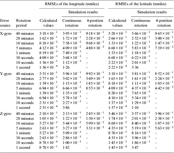
5.2. Simulations of Position Errors' Response to Gyros' First-order Markov Processes
Equations (19) to (24) show the RMSEs of the longitude and the latitude produced by each gyro's first-order Markov process in an INS, and Equations (33) to (38) are for a RINS. In order to test the usability of the derived formulae, the simulation conditions are set as follows: a first-order Markov process is added to each axis gyro's value in an INS and a RINS. Its correlation time is 3600 seconds and SD is 0·01°/h; in the RINS, the rotation period is set as 40 minutes, 20 minutes, 10 minutes, 5 minutes, 1 minute, 30 seconds, 10 seconds and 1 second respectively. Besides, for the rotation period with 40 minutes, 20 minutes, 10 minutes and 5 minutes, both the continuous rotation mode and the four-position rotation mode are considered; for the rotation period of 1 minute, 30 seconds, 10 seconds and 1 second, only the continuous rotation mode is considered, since the above rotation periods are short and not suitable for the four-position rotation mode.
The simulation results are shown as Tables 2 and 3, which are the statistical results of 100 simulations. Figures 7 to 12 show the RMSE curves of the simulated INS and the simulated RINS with the rotation period as 20 minutes.
Figure 7. The RMSEs of the longitude response to the X-gyros first-order Markov process.
Figure 8. The RMSEs of the latitude response to the X-gyro's first-order Markov process.
Figure 9. The RMSEs of the longitude response to the Y-gyro's first-order Markov process.
Figure 10. The RMSEs of the latitude response to the Y-gyro's first-order Markov process.
Figure 11. The RMSEs of the longitude response to the Z-gyro's first-order Markov process.
Figure 12. The RMSEs of the latitude response to the Z-gyro's first-order Markov process.
Table 2. The final RMSEs of the position response to gyros' first-order Markov process in the INS.

Table 3. The final RMSEs of the position response to the gyro's first-order Markov process in the RINS.
From Figures 7 to 12, it can be observed that the trends of the calculated results are consistent with the simulation results. The final RMSEs of the position are shown in Tables 2 and 3 and the following conclusions can be drawn:
1) The simulation results of the RINS adopting the continuous rotation mode show good consistency with the calculated values except for the one with the rotation period as one second. It indicates that the derived formulae are valid in most ranges of rotation periods. However, when the rotation period reaches the sample time, the rotation technique fails because of insufficient samples.
2) Comparing the simulation results of the RINS adopting the four-position rotation mode with the calculated values, it can be seen that the RMSEs of the simulation results are larger than the calculated ones. However, the difference decreases as the rotation period decreases. When the rotation period is 20 minutes, the RMSEs of the simulated results are about 1·3 times the calculated ones, which is accurate enough for the analysis of the compensation effects in the RINS.
6. CONCLUSIONS
In this paper, the compensation effects of gyros' stochastic errors achieved by the rotation technique in a RINS are discussed. During the research, the position errors of an INS and a RINS response to gyros' stochastic errors, which are modelled as GW noise plus first-order Markov process, are analysed. The error propagation formulae are derived, as shown in Equations (9) to (14), (19) to (24) and (33) to (38). A variety of different simulation conditions were designed to test the formulae. Through the theoretical analysis and the simulation results, the following conclusions can be made:
1) The rotation technique has no compensation effect for the position error produced by gyros' GW noises. In a RINS, the error propagation characteristics of gyros' GW noises to the position error are the same with the characteristics in an INS, shown as Equations (9) to (14).
2) The rotation technique has good compensation effect on the position error produced by gyros' first-order Markov processes. Adopting the continuous rotation scheme, the quantitative formulae are derived as Equations (33) to (38), and it is proved that the compensation effect improves as the rotation period decreases. When an actual rotation mode (such as the four-position rotation mode) is adopted, the compensation effect is lower than the derived formulae. However, the derived formulae are accurate enough to analyse the compensation effects brought by the rotation technique.
Currently, two types of RINSs, including a fibre optic gyro (FOG) -based RINS and a micro electro mechanical system (MEMS) gyro based RINS, are being designed in the authors' department. The theoretical results of this paper have been applied to the design phase: firstly, since the position errors of the RINS produced by gyros' stochastic errors can be quantitatively predicted, the derived formulae were used to guide the type selection of gyros according to the expected navigation accuracy; secondly, static experiments of the selected gyros were carried out and gyros' stochastic errors were analysed, and then the theoretical results of this paper were used during the design of the two RINSs' rotation schemes. The theoretical results have potential application in the design of other INSs and RINSs.
Although the theoretical results of this paper serve as an important reference for the design of a rotation scheme, it should be stated that there are still many other factors to consider, such as the compensation effects of IMU's other errors and the errors introduced by the rotation.
FINANCIAL SUPPORT
This work was supported by the National Natural Science Foundation of China, (Jizhou Lai, grant number 61174197); the Funding of Jiangsu Innovation Program for Graduate Education (Pin Lv, grant number CXLX11_0201); and the Funding for Outstanding Doctoral Dissertation in NUAA (Pin Lv, grant number BCXJ11-04).