


Introduction
Recently, through-the-wall radar imaging (TWRI) has found wide applications in searching and rescuing missions of civilian: earthquake, hostage, and fire, among others [Reference Amin1–Reference Wu, Zhou, Liu and Duan4]. TWRI facilitates detection, localization, and classification of objects behind opaque structures [Reference Abdalla, Alkhodary and Muqaibel5–Reference Liu, Gu and So8]. Because of their massive applications in delicate tasks, current studies in TWRI focus on producing highly resolved radar images of the scenes of interest. Large radar apertures and wide signal bandwidths are required to achieve highly resolved images in crossrange and downrange, respectively. These requirements translate to large sensing measurements that limit the applications of TWRI [Reference Yoon and Amin9, Reference Amin and Ahmad10]. Therefore, researchers in TWRI applied compressive sensing (CS) technique to compresses the sensed signal during data acquisition. Thus, compressed sensing enables image reconstruction using fewer measurements than those dictated by the Nyquist sampling theorem, provided that the signal of interest is sparse or exhibits sparsity in some transform domain [Reference Donoho11–Reference Candes and Tao13].
Three major approaches exist to solve the CS reconstruction problem, namely convex optimization, greedy, and Bayesian [Reference Abdalla, Alkhodary and Muqaibel5, Reference Wipf and Rao14].Optimization-based approaches usually use ℓ1-norm [Reference Liu, Yang, Gu and So15], and, given the noisy through-the-wall measurements, researchers find the Basis Pursuit De-Noising as a more suitable convex optimization method [Reference Candes and Tao13]. Under particular situations, ℓ1/ℓ2-norm may be employed to achieve better reconstruction [Reference Leigsnering, Ahmad, Amin and Zoubir7]. Greedy approaches solve the reconstruction problem iteratively until a stopping criterion is attained. Greedy algorithms, such as Orthogonal Matching Pursuit [Reference Guang and Qi16] and Subspace Pursuit give lower execution times. But such algorithms dictate stricter sparsity conditions, and hence are non-optimal [Reference Donoho, Tsaig, Drori and Starck17, Reference Dai and Milenkovic18]. While the previous methods use signal sparsity as the only prior information, Bayesian approaches improve signal recovery through noise statistics (when available). In Bayesian algorithms, the unknown signal is modelled as Bernoulli–Gaussian or Bernoulli–Laplacian [Reference Masood and Al-Naffouri19, Reference Abdalla20].
Although CS uses fewer measurements to reconstruct a signal, the downside of CS is that it lifts the computational burden from the sensing stage while reinvigorate burden on recovery stage, which results in highly computationally expensive recovery of signals. This limitation obscures practical applications of CS in TWRI. Therefore, faster algorithms are needed to ensure that we elevate the capabilities of TWRI in real-world sensitive applications.
This work proposes the use of numerical optimization method, Limited-memory Broyden–Fletcher–Goldfarb–Shanno (LBGFS) in conjunction with Tikhonov regularization, to recover an unknown image vector from compressed TWRI measurements. Limited Memory Broyden–Fletcher–Goldfarb–Shanno (LBFGS) offers affordable computational cost, demands less memory, and provides faster convergence time, but these potential advantages have not been fairly utilized in complex TWRI applications [Reference Bonnans, Gilbert, Lemaréchal, Sagastizábal, Casacuberta, Greenlees, MacIntyre, Sabbah, Süli and Woyczyński21, Reference Sun, Chen and Qu22]. In [Reference Sun, Chen and Qu22], the authors proposed an interesting image reconstruction method based on LBFGS and Particle Swarm Optimization algorithm (LBFGS_PSO) to reconstruct image under wall parameters uncertainties. The focus of the paper was to determine wall parameters while reconstructing stationary and moving targets. The reconstruction time, however, was not studied. Further, their model does not consider target-to-target interaction making it ineffective in multiple targets scenarios that is inevitable in TWRI applications. Our work, therefore, gives a promising future for the realization of TWRI in critical applications that could otherwise not be accomplished using traditional approaches.
TWRI scene model
In this study, the interrogation of the TWRI scene involves a stepped frequency radar (SFR). Among advantages of SFR is that, it helps to maintain high energy of the transmitted ultra-wideband (UWB) signal and hence improves signal-to-noise ratio (SNR) [Reference Muqaibel, Abdalla, Alkhodary and Al-Dharrab23].
Consider SFR with N different radar positions; at each position of the radar, M monochromatic signals, equally spaced in frequency, are transmitted and received to realize an UWB signal. Figure 1 shows a multiple-targets scene divided into N x and N y pixels in crossrange and downrange, respectively. The target reflectivity is denoted by σ p, with p = 0, 1, …N xN y − 1, and wall reflectivity is denoted by σ w. If target returns and wall returns are R and R w, respectively, then the received signal, y[m, n], at the n th radar location when the m th frequency is transmitted is given as Muqaibel et al. [Reference Muqaibel, Abdalla, Alkhodary and Al-Dharrab23, Reference Abdalla, Muqaibel and Al-dharrab24].

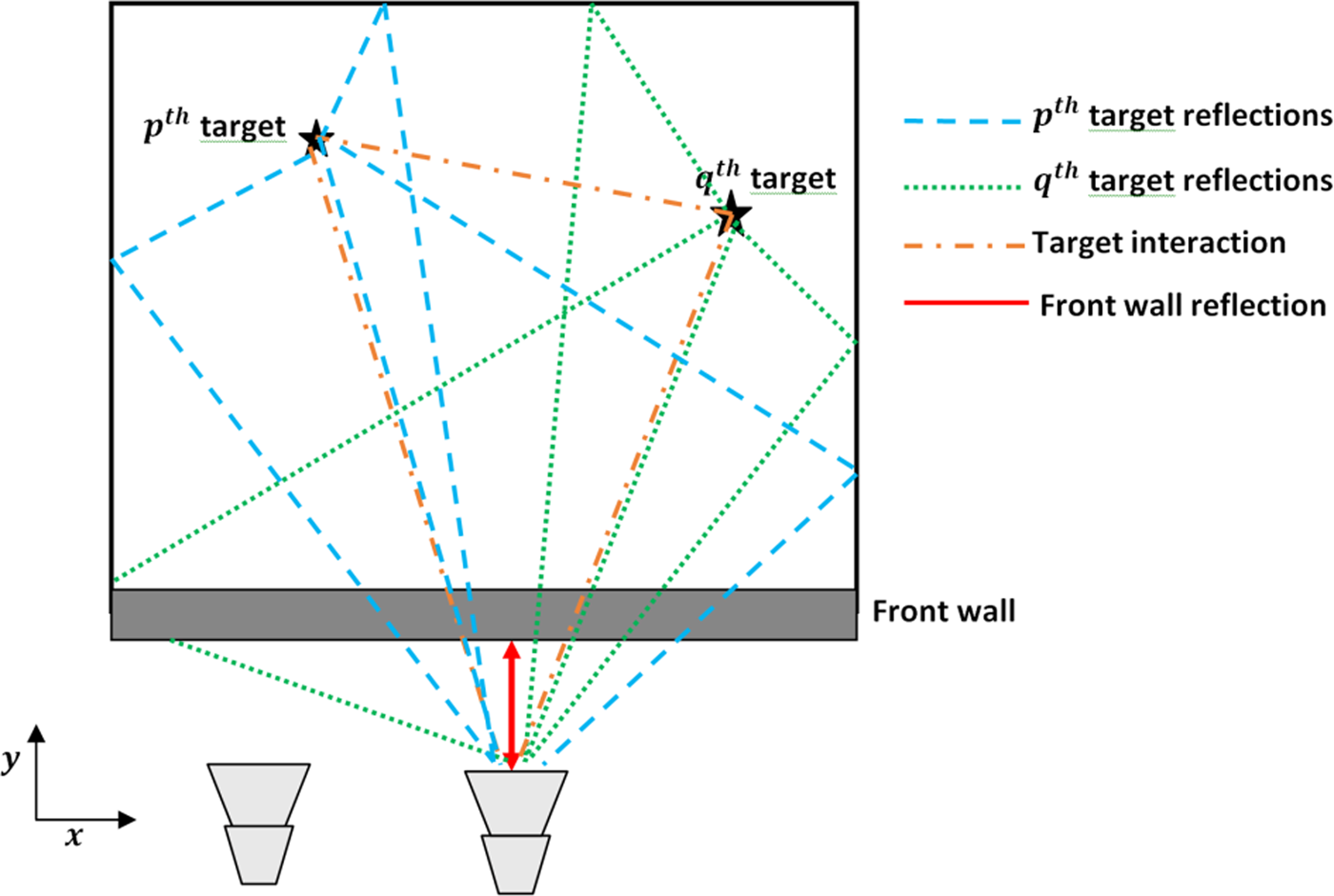
Fig. 1. Multiple targets with first-order returns.
Source: [Reference Muqaibel, Abdalla, Alkhodary and Al-Dharrab23].
Proposed reconstruction method
CS reconstruction algorithms
Several compressed sensing algorithms have been proposed in the literature, but only a few were applied in TWRI. Among these algorithms, Your Algorithm for ℓ1 optimization (YALL1) has become popular to solve ill-posed systems. In [Reference AlBeladi and Muqaibel25], compressed sensing algorithms in TWRI were tested under the F1-score, and YALL1 yielded the best performance in low SNR values. In addition, YALL1 achieved higher quality values when the compression rate was reduced to 50%. Consequently, researchers have declared that YALL1 spans the widest region within the desired performance values for the given SNR and compression ratio.
Despite its higher performance, YALL1 considers all elements in the unknown vector to generate a solution. This operation adds computational load of the algorithm unnecessarily, and hence slows down the process of reconstructing an image. Recalling large matrices in the TWRI problem, YALL1 may take a longer reconstruction time.
LBFGS optimization method in TWRI
The Broyden–Fletcher–Goldfarb–Shanno (BFGS) algorithm is a quasi-Newton algorithm known for its super-linear convergence [Reference Dai and Milenkovic18, Reference Nocedal and Wright26]. The algorithm is well presented in [Reference Bonnans, Gilbert, Lemaréchal, Sagastizábal, Casacuberta, Greenlees, MacIntyre, Sabbah, Süli and Woyczyński21] and [Reference Nocedal and Wright26]. The function, J, to be minimized by BFGS is approximated with the quadratic model (2):

Where Bk is an n × n symmetric positive definite Hessian matrix that is updated at every iteration, p denotes the minimizer, and T denotes the transpose. The value of sk is then updated as:

where $p_k = {-}{\boldsymbol B}_k^{{-}1} \nabla J( {\boldsymbol s})$ is the direction vector, α k is the fixed step length at iteration k. The choice of α k depends on the Wolfe conditions:

and

where (c 1, c 2) ∈ ℝ2; c 1 ∈ (0, 1) and c 2 ∈ (c 1, 1). In practice, c 1 is set to a very small number; for example c 1 = 10−4 [Reference Nocedal and Wright26]. On the other hand, the value of the step length (line search parameter), α k, can be computed using an exact line search method in [Reference Nocedal and Wright26].
The Hessian matrix can iteratively be approximated to give the David–Fletcher–Powell equation

where

Imposing a condition on the inverse Hessian matrix, ${\boldsymbol H}_k = {\boldsymbol B}_k^{{-}1}$ , we obtain an update BFGS equation

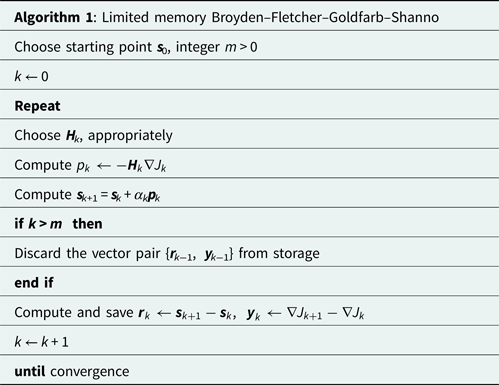
As a way of increasing the computational efficiency, LBFGS approximates the Hessian matrix by storing the most recent m vectors from k iterations [Reference Nocedal and Wright26]. Thus, setting ${\boldsymbol V}_k = {\boldsymbol I}-\rho _k{\boldsymbol s}_k{\boldsymbol y}_k^T$ gives
gives

Expanding (8) allows efficient computation of the product ${\boldsymbol H}_k\nabla J_k$ needed in sk update without storing the full matrix, Hk.
Both LBFGS (Algorithm 1) and BFGS give the same results within the first (m − 1) iterations for ${\boldsymbol H}_k^0 = {\boldsymbol H}_0$ . Complete details of various quasi-Newton methods, including LBFGS, can be found in [Reference Broyden27–Reference Xiao, Wei and Wang31].
Least-squares method
Well-posed problems are solvable and give unique solutions that depend continuously on system parameters. Ill-posed problems lack these constrains, and can emerge from inverse problems that prevail in science and engineering fields, such as signal processing, acoustics, and image processing [Reference Kim, Koh, Lustig, Boyd and Gorinevsky32].
This work presents an ill-posed problem (also called under-determined system) that contains a system of linear equations with fewer equations than unknowns [Reference Wei, Li and Qi30, Reference Figueiredo, Nowak and Wright33]. The general representation of the ill-posed problem is

with ${\boldsymbol A}\in {{\mathbb R}}^{a \times b}$ denoting a mapping matrix that maps a state vector, s ∈ ℝb, to give y ∈ ℝa, where a and b represent number of rows and columns of A. From (9), the ℓ2 minimization problem to compute the cost function, J(s), becomes

Equation (10) can be written in matrix form as:

Then, to obtain the gradient, J(s) is differentiated as:

Hence,

Or

The LBFGS algorithm requires the cost function, J(s), and its gradient as inputs. In this study, the value of J(s) is computed by the least-squares method based on the Euclidean norm. Then, regularization process follows, whereby a value is added to the cost of function to provide a proper search direction of the optimal solution.
Proposed regularization function
Regularization methods provide means to solve linear inverse problems in science and engineering fields [Reference Calvetti, Morigi, Reichel and Sgallari34]. Tikhonov regularization is the simplest and oldest form of regularization that has been widely applied by researchers as it gives convincing results at lower computational load [Reference Golub, Hansen and O'Leary35]. Tikhonov regularization offers an improved efficiency in exchange for a tolerable bias in problems involving parameter estimation or in models with large number of parameters.
Consider the ill-posed equation (9). Then, Tikhonov regularization requires re-formulation of the equation by introducing Tikhonov term that prevents degeneration of the solution. Therefore, the equation re-formulation gives

where μ ≥ 0 denotes a regularization parameter that determines the amount of regularization, and I is the identity matrix. Using ordinary least-squares method, J(s)derived from (15) becomes

where Γ = μ I. This regularized cost function in (11) and the gradient in (14) are used as inputs to the proposed optimization method.
Results and discussion
Simulation results
The room layout was maintained as that in the work of [Reference Kokumo, Abdalla and Maiseli36], and the coordinate system's origin is the center of the array (Fig. 2). The front wall was located at 0.5 m parallel to the array with thickness of 20 cm. The first target was placed at (0.31, 3.6) m, the second target was added at (−0.62, 5.2) m, third target was placed at (0.71, 1) m and the fourth target was introduced at (2.5, 4.0) m as shown in Fig. 2. Computer with Intel® core™ i7-8550U CPU @ 1.80 GHz 1.99 GHz processor, 16.0 GB RAM, a 64-bit Operating System, x64-based processor and the windows edition installed was windows 10 pro and MATLAB R2019a software was used for performing the simulation. Next, the targets were reconstructed using LBFGS, configured to run through 30 iterations with 15 stored vectors. Empirical experiments show that this configuration guarantees optimal reconstruction results. Furthermore, we set the step length to 5.5 and the initial Hessian was an identity matrix.

Fig. 2. Measurement setup and room layout.
In each scenario, the targets were reconstructed and performance measures were compared with the state-of-the-art method presented in [Reference Kokumo, Abdalla and Maiseli36]. The parameters set for imaging were as follows: frequency range (f) = 1 − 3 GHz; frequency bins (M) = 801; transceiver locations (N) = 77; and number of multipath (R) = 4. Finally, the scene was discretized into 64 × 64 pixels.
Scenario 1: Varying number of targets
In this scenario, we started by reconstructing the first two targets using the existing and proposed methods. Figures 3(a) and 3(b) show the final images for two-target reconstruction using the existing method and the proposed method. Figures 4(a) and 4(b) show reconstructed images using three targets for the existing and the proposed method. Figures 5(a) and 5(b) show the final images with four targets reconstructed using existing method and the proposed method. By visual inspection, the figures in all the three cases seem to have nearly the same quality.

Fig. 3. Reconstructed images for two targets. (a) Existing method. (b) Proposed method.

Fig. 4. Reconstructed images for three targets. (a) Existing method. (b) Proposed method.

Fig. 5. Reconstructed images for four targets. (a) Existing method. (b) Proposed method.
To quantify the performance, RT, MSE, SCR and RCP were used. Figure 6(a) shows that the proposed method reconstructs the image within a shorter time compared with the existing method. Also, Fig. 6(b) shows that the existing method gives images with relatively lower MSE when the numbers of targets is small. However, as the number of targets increases, our proposed method demonstrates better performance in terms of MSE relative to the existing method. Figures 6(c) and 6(d) show that the existing method outperforms the proposed method, in terms of SCR and RCP, but visual results suggest that our method maintains acceptable perceptual qualities.

Fig. 6. Variation of performance measures with the number of targets. (a) RT, (b) MSE, (c) SCR and (d) RCP.
Scenario 2: Varying the size of the data volume
In this scenario, four targets were chosen and kept constant throughout the experiment, a situation seen in Fig. 2. Data volumes considered in this case were 10, 12.5, 16, and 25%. The aim of this experiment was to establish the effect of data volume to the performance of the reconstruction algorithm. To quantify the performance, again run time, MSE, RCP, and SCR were used as performance indicators. Figures 7(a) and 7(b) show the images of the scene reconstructed at 10% data volume using the existing and proposed method. Again, the visual appearance of the two images is almost similar. However, qualitatively the proposed method demonstrates better performance over a wide range of values.

Fig. 7. Reconstructed images with 10% data volume. (a) Existing method. (b) Proposed method.
The results in Fig. 8(a) show that the proposed method offers lower run time compared with the existing counterpart. It was observed that the run time, for both methods, increases with data volume. Though, the existing method returned lower MSE value, Fig. 8(b) shows that as the data volume increases, MSE of the proposed method decreases significantly. Figures 8(c) and 8(d) show the variations of SCR and RCP with the data volumes. It is evident from the figures that the existing proposed method produces relatively high SCR and RCP. In summary, we have achieved lower run time at the expense of the image quality. Nevertheless, the reconstructed images using the proposed method have acceptable qualities and can be clearly interpreted. We can therefore, argue that our method can be sought out in real-world applications where the response time is very crucial, including rescue missions and military surveys.

Fig. 8. Variation of performance measures with the data volume. (a) RT, (b) MSE, (c) SCR and (d) RCP.
Scenario 3: Varying SNR
The intention of this scenario was to examine the robustness of the proposed method relative to the existing one. In this case, four targets were considered for the reason similar to that explained in the previous experiment. The targets were reconstructed at different SNR values ranging from 0 to 20 dB. Figures 9(a) and 9(b) show the images reconstructed with the existing and proposed methods when the value of SNR was set to 0 dB. The image of the existing method is highly cluttered compared with the proposed method.

Fig. 9. Image reconstruction at 0 dB SNR. (a) Existing method. (b) Proposed method.
Figure 10(a) shows the run times at different SNR values where the proposed method exhibits lower run times for all SNR. Figure 10(b) shows the values of MSE at different SNR values and the results indicate that the proposed method outperforms the existing method over a wide range of SNR values. In Fig. 10(c), our method gives higher SCR values for a wide range of SNR values compared with the existing one. However, the two give comparable RCP values as shown in Fig. 10(d). Generally, this observation alludes that the proposed method is highly effective under noisy environment, and hence more suitable in practical TWRI scenarios.

Fig. 10. Variation of performance measures with SNR. (a) Run Time, (b) MSE, (c) SCR and (d) RCP.
Experimental results
In order to further evaluate the performance of the proposed method, experimental data were employed in the LBFGS method. The used experimental data were obtained from King Fahd University of Petroleum and Minerals (KFUPM). The experimental setup involved two targets of radius 23 cm located at (0.75, 2) m and (0.5, 3) m [Reference Muqaibel, Abdalla, Alkhodary and Al-Dharrab23]. The results were fairly compared with the existing method. Figures 11(a) and 11(b) show the images reconstructed with the existing and proposed methods, respectively, at different data volumes. It is revealed that the visual image quality of proposed method is acceptable though it is slightly lower than that of existing method. Quantitative results, presented in Fig. 12, support the observation.

Fig. 11. Reconstructed images using with experimental data. (a) Existing method. (b) Proposed method.

Fig. 12. Variation of performance measures with the data volume using experimental data. (a) Run time, (b) MSE, (c) SCR and (d) RCP.
The results in Fig. 12(a) show that the run time, for both methods, increases with data volume and the proposed method attains lower run time compared to the existing method at the expense of image quality. It is observed in Fig. 12(b), the existing method returns lower MSE value at lower data volumes. As the data volume increases, MSE of the proposed method decreases significantly. Figures 12(c) and 12(d) respectively show the variations of SCR and RCP with the data volumes. It is evident from Fig. 12 that the proposed method returns relatively low, but acceptable, SCR and RCP. The run time for the proposed method has proved to be significant, thus making it more suitable in time-sensitive operations, such as rescue missions.
Conclusion
The authors of this study have introduced a fast image reconstruction method in TWRI. The method uses LBFGS optimization as a sub-problem in the least-squares problem. Simulation results demonstrate that the proposed method executes faster relative to the existing method. Furthermore, our method generates plausible scenes that closely match with the reference scenes. Using objective quality metrics (MSE, SCR, and RCP), the proposed method outperforms the classical method without sacrificing the computational load. Therefore, our method performs reconstruction faster without degrading quality of the reconstructed image. This promising achievement may have a significant positive impact on the application of TWRI in real situations. Currently, we are extending the method to incorporate extended targets scenarios.
Acknowledgements
The authors would like to extend their sincere gratitude to the University of Dar es Salaam for funding this work through the project number COICT-ETE 19048. In addition, we feel indebted to the College of Information and Communication Technologies for the support to complete the write-up of the manuscript. Further, we would like to sincerely express our appreciation to Prof. Ali Muqaibel's research lab at KFUPM for providing experimental data that made our contribution more suitable for the readers.
 Candida Mwisomba received B.Sc. degree in electronics and communication engineering, from St. Joseph University, Tanzania, in 2017 and M.Sc. in electronics engineering and information technology from the University of Dar es Salaam, Tanzania in 2020. Her research interests are in signal processing, particularly through-the-wall radar imaging and sparse reconstructions.
 Abdi T. Abdalla received the B.Sc. degree in electronic science and communication and M.Sc. degree in electronics engineering and information technology from the University of Dar es Salaam, Tanzania, in 2006 and 2010, respectively, and the Ph.D. degree in electrical engineering majoring in communication and signal processing, from King Fahd University of Petroleum and Minerals (KFUPM), Saudi Arabia, in 2016. Currently, he is a senior lecturer at the Department of Electronics and Telecommunications Engineering, University of Dar es Salaam, Tanzania. His research interests include through-the-wall radar imaging, indoor target localization, sparse arrays processing, application of compressive sensing to radar signal processing, and radio frequency energy harvesting. Dr. Abdalla received many awards in the excellence in teaching, researching, and supervising graduate students.
 Idrissa S. Amour received the B.Sc. with education degree in physics and mathematics and M.Sc. degree in technomathematic from the Lappeenranta University of Technology, Finland, in 2008 and the Doctor of Science degree in applied mathematics from the Lappeenranta University of Technology, Finland, in 2016. Currently, he is a lecturer at the Department of Mathematics of the University of Dar es salaam. His research interests include mathematical modelling, numerical weather predictions, simulation, digital assessments in mathematics.
 Florian Mkemwa received his B.Sc. and M.Sc. degrees in telecommunications engineering, both from the University of Dar es Salaam (UDSM), Tanzania, in 2014 and 2020, respectively. Since 2016 he has been with the University of Dar es Salaam where he is serving as a tutorial assistant in the Department of Electronics and Telecommunications Engineering. His research interests focus on signal processing, particularly in through-the-wall radar imaging.
 Baraka J. Maiseli earned his Doctoral degree in 2015 from the Harbin Institute of Technology (HIT), PR China, where he was also awarded the honorary certificate as the best international scholar of the year. Between 2015 and 2017, he worked with HIT as a postdoctoral researcher. Maiseli has published several articles in referred Journals, and is a verified peer reviewer for various international journals: IEEE Transactions on Industrial Electronics, Neurocomputing, IET Biometrics, Signal Processing, and International Journal of Remote Sensing, among others. His research interests are in machine learning, computer vision, image and video processing, artificial intelligence, and embedded electronics. Currently, Maiseli works at the University of Dar es Salaam (UDSM), Department of Electronics and Telecommunication Engineering, as a senior lecturer. With more than 13 years of teaching experience at UDSM, Maiseli has been supervising both undergraduate and postgraduate students in their projects, research, and practical training.


