1. Introduction
Vortex rings (Shariff & Leonard Reference Shariff and Leonard1992) have always played a crucial role in scientific research and engineering applications. Over the past few decades, the dynamics of the vortex ring evolving in a uniform environment has been well established in theory (Shusser & Gharib Reference Shusser and Gharib2000; Krueger Reference Krueger2005; Sullivan et al. Reference Sullivan, Niemela, Hershberger, Bolster and Donnelly2008), experiment (Maxworthy Reference Maxworthy1977; Glezer Reference Glezer1988; Cater, Soria & Lim Reference Cater, Soria and Lim2004; Das, Bansal & Manghnani Reference Das, Bansal and Manghnani2017) and numerical simulation (Shariff, Verzicco & Orlandi Reference Shariff, Verzicco and Orlandi1994; Archer, Thomas & Coleman Reference Archer, Thomas and Coleman2008; Lin et al. Reference Lin, Xiang, Xu, Liu and Zhang2020). However, for many practical situations, the formation and evolution of the vortex exist in a non-uniform or stratified environment, such as the wake of aircrafts and vessels in the stratified flow, convection of thermals in the inversion layer, interaction of flame fronts with the turbulent flow, diffusion of contaminants in the atmosphere and halocline in oceans (Dahm, Scheil & Tryggvason Reference Dahm, Scheil and Tryggvason1989; Sarpkaya Reference Sarpkaya1996; Advaith et al. Reference Advaith, Manu, Tinaikar, Chetia and Basu2017). As a result, the dynamics of the vortex ring can be more complex under the influence of the interaction with the stratified interface. Therefore, it is of importance to understand the dynamics and mechanism for flow control by manipulating the vortex ring.
The canonical property during the vortex ring impinging on a stratified interface is the generation of the secondary or tertiary vorticity in non-zero density gradient regions due to baroclinicity. The interactions between different vortical structures have a profound impact on the vortex dynamics involving rebounding, reconnection, destabilization and collapse (Song, Bernal & Tryggvason Reference Song, Bernal and Tryggvason1992; Advaith et al. Reference Advaith, Manu, Tinaikar, Chetia and Basu2017), as well as entrainment and mixing (Linden Reference Linden1973). In addition to the complex interaction phenomena, the flow field properties are influenced by multiple control parameters, including Reynolds number (Re), Atwood number (At), Froude number (Fr) and Richardson number (Ri). The Atwood number gives the non-dimensional density difference across the interface (Dahm et al. Reference Dahm, Scheil and Tryggvason1989), Froude number measures the competition beween the inertial force and the restoring buoyancy force (Herault, Facchini & Bars Reference Herault, Facchini and Bars2018), and Richardson number denotes the ratio of the potential energy of the stratification and the kinetic energy (Olsthoorn & Dalziel Reference Olsthoorn and Dalziel2017). The formation of the secondary or tertiary vortex ring is also universal in the vortex ring interaction with solid boundaries (Walker et al. Reference Walker, Smith, Cerra and Doligalski1987; Orlandi & Verzicco Reference Orlandi and Verzicco1993; Cheng, Lou & Luo Reference Cheng, Lou and Luo2010; Xu et al. Reference Xu, He, Kulkarni and Wang2017). However, the generation mechanism for the latter is attributed to boundary layer separation under the adverse pressure gradient (Walker et al. Reference Walker, Smith, Cerra and Doligalski1987).
The research of the vortex dynamics in a stratified environment has been mainly conducted with respect to the laminar or turbulent vortex ring impinging on a free surface or an internal interface. For the interaction with a free surface, Chu, Wang & Hsieh (Reference Chu, Wang and Hsieh1993) experimentally compared the dynamics of a laminar vortex ring impinging on a free surface and a solid surface at the circulation Reynolds numbers  $Re_{\varGamma} $ from 900 to 2350. They found the fundamental flow phenomenon of the primary vortex ring was similar between the two cases, which could be divided into three stages of vortex free-traveling, stretching and rebounding. However, with increasing Reynolds number, the free surface deformation was enhanced to reach approximately 4 % of the orifice diameter despite a lower Froude number (Fr < 0.15).
Song et al. (Reference Song, Bernal and Tryggvason1992) investigated the free surface waves generated by the head-on collision of a vortex ring at  $Fr = 0.252\unicode{x2013}0.988$ and
  $Re_{\varGamma} = 15\;100\unicode{x2013}64\;700$ by experiment and numerical simulation. They observed three types of free surface patterns associated with the vortical structure evolution, including axisymmetric depression of the surface for weak vortex–surface interaction, axisymmetric radially propagating waves in the early stage of strong vortex–surface interaction and fully three-dimensional (3-D) waves with breakup of the vortex core. Particularly, they detected vortex reconnection as the main cause of the generation of the surface waves after colliding with the surface. Vortex reconnection was further studied by Weigand & Gharib (Reference Weigand and Gharib1995) for a turbulent vortex ring impinging on the free surface with various angles at Fr = 0.46. The flow field exhibited a trifurcation that resulted from the interaction with the surface during the transition stage, and a bifurcation during the fully developed turbulent stage. However, the reconnection was absent in the simulation of Archer, Thomas & Coleman (Reference Archer, Thomas and Coleman2010) for a laminar vortex ring impinging on a free surface with Fr approaching zero. They ascribed this discrepancy to the effects of the slenderness ratio, initial depth and Reynolds number of the vortex ring.
In terms of the interaction with an internal interface between two liquids, Linden (Reference Linden1973) earlier experimentally studied entrainment caused by a turbulent vortex ring impinging on a density interface with Fr between 0.14 and 0.80. They found that the maximum penetration length of the vortex ring was a function of Fr. Dahm et al. (Reference Dahm, Scheil and Tryggvason1989) performed a detailed flow visualization of an axisymmetric vortex ring interaction with a variable thickness interface at  $Re_{\varGamma} = 2000\unicode{x2013}16\;000$. The density difference was sufficiently small to satisfy the Boussinesq limit, and Ri (= Fr −2) varied from 4.3 to 275. The results indicated that for a sharp interface (the interface thickness was far less than the vortex length scale), the vortex dynamics was governed solely by AR, i.e. the product of At and Ri. At a lower AR, the outmost layer of the vortex ring was successively peeled away by baroclinic vorticity, resulting in the formation of a complex backflow. In contrast, the dynamics tended to the interaction with a solid wall with the increased AR. However, for a thick interface, the vortex dynamics was also related to the interface thickness.
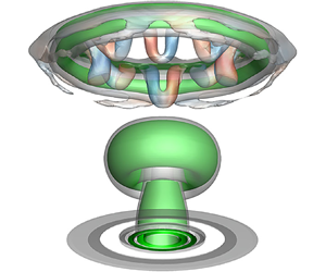
Orlandi, Egermann & Hopfinger (Reference Orlandi, Egermann and Hopfinger1998) presented experimental and numerical results of a laminar vortex ring descending in a density fluid with finite thickness. The vortex ring was observed to shrink as it penetrated the stratified fluid, and eventually disappeared due to the effects of baroclinic vorticity and cross-diffusion, whereas no internal waves were generated. In a similar stratified environment, Advaith et al. (Reference Advaith, Manu, Tinaikar, Chetia and Basu2017) studied the vortex behaviour by particle image velocimetry (PIV) over a range of Re = 1350–4600 and Ri = 0.1–4. The scenarios of the vortex–interface interaction were characterized into non-penetrative, partially penetrative and extensively penetrative regimes. In addition, they detected the occurrence of short-wavelength instability for a plume structure generated by the vortex ring against buoyancy. Olsthoorn & Dalziel (Reference Olsthoorn and Dalziel2017) investigated the mechanism of the vortex ring interaction with a stratified interface at Re = 1600–2800 and Ri = 0.6–9.8. The reconstruction of the three-dimensional vortical structures based on stereoscopic PIV enabled analysis of the vortex ring instability. The results indicated that the unstable wavenumber in the presence of a stratified interface was similar to the unstratified situation, and the time scale of the instability growth was inversely dependent on Ri. Furthermore, the instability of the secondary vorticity field was similar to the Crow instability.
Compared to the stratified environment constructed by two miscible liquids with some cross-diffusion, the interface between two immiscible liquids also exists in many applications including petroleum transportation, oil spills on the sea, two-phase reactions and separations in industries (Park, Chinaud & Angeli Reference Park, Chinaud and Angeli2016; Song, Choi & Kim Reference Song, Choi and Kim2021). However, the interaction of the immiscible interface with the external perturbance of a jet or a vortex ring has been rarely brought into focus, which involves complex interface behaviours in addition to the vortex dynamics. Recently, Yeo et al. (Reference Yeo, Koh, Long and New2020) conducted an experiment of a vortex ring colliding with a sharp water–oil interface at Re = 1000–4000. The results indicated that the flow pattern was directly influenced by the Reynolds number, where the degree of the interface deformation was enhanced with increasing Reynolds number. At the largest Reynolds number, the vortex ring could penetrate the interface almost completely, and then reversed its translational direction with the formation of a trailing jet due to the buoyancy effect. However, there is still a lack of quantitative analysis on the vortex dynamics, as well as the accurate tracking of the interface deformation and possible interfacial waves. In addition, Song et al. (Reference Song, Choi and Kim2021) experimentally studied the behaviours of the water–oil interface with an impinging vortex ring generated in oil. They identified the key features of the interface in a non-dimensional regime map as no-deformation, no-rebounding, rebounding and symmetry breakup. The geometric quantities related to the interface deformation were characterized by the Froude and Bond numbers. However, they only measured the 2-D velocity fields in the oil layer. The details of the vortical structure evolution near the interface and three-dimensional properties of the interface, especially for a strong vortex–interface interaction, remain to be explored.
The purpose of this study is to investigate the dynamics of the interaction of successive vortex rings with a stratified water–oil interface by experiment and numerical simulation. The previous studies mainly focus on an isolated vortex ring impinging on the stratified interface. In a practical flow system, the evolution and deformation of the interface are usually an accumulated consequence of persistent vortex–interface interactions. Furthermore, the interaction between vortex rings could be more complex than that for an isolated situation. Based on these perspectives, we use a synthetic-jet actuator (Smith & Glezer Reference Smith and Glezer1998; Cater & Soria Reference Cater and Soria2002; Glezer & Amitay Reference Glezer and Amitay2002; Wang & Feng Reference Wang and Feng2018) to periodically generate vortex rings so that successive vortex–interface interactions can be achieved. In particular, the application of 3-D numerical simulation enables accurate capture of the 3-D instability of vortex rings and the spatio-temporal properties of the interface, and thus gain insight into the underlying flow mechanism.
2. Experimental setup and procedures
2.1. Experimental setup and parameters
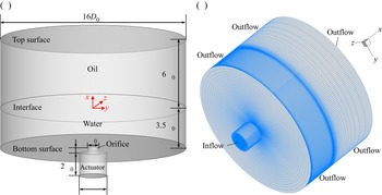
The experiments were performed in a Plexiglas water tank of 600 × 600 × 600 mm3 with a room temperature of 27 °C. The vortex ring was generated by a piston-type synthetic jet actuator (Xu et al. Reference Xu, He, Kulkarni and Wang2017; Wang, Feng & Xu Reference Wang, Feng and Xu2019) which was made up of a Panasonic servo electromotor (MSMD042PIU), an eccentric disk, a connecting rod with length l = 300 mm, a piston with diameter Dp = 29 mm and a cavity, as shown in figure 1. A hard rubber hose was used to connect the synthetic jet actuator and a J-like Plexiglas hollow circular cylinder to ensure sealing. The hollow circular cylinder was approximately 300 mm from the tank bottom. A circular jet orifice with diameter D 0 = 12 mm and plate thickness Hp = 5 mm was mounted on the end of the hollow circular cylinder so that the vortex rings coud move upwards vertically during the experiments. Note that the vertical segment of the hollow circular cylinder close to the jet orifice was 120 mm (10D 0), and that was long enough to eliminate any possible impact of the bent segment on the formation of the vortex ring.

Figure 1. Schematic of experimental set-up for LIF and PIV measurements.
Before the experiments, the tank was first filled with water up to the height Hw = 42 mm (3.5D 0) above the orifice. The water had been filtered using a filter with a carbon-fiber filter element and filtering precision of 5–10 μm, guaranteeing less impurities within the water. After that, soy oil with  ${\rho _o} = 915.8\;\textrm{kg}\;{\textrm{m}^{ - 3}}$ and
  ${\mu _o} = 0.0413\;\textrm{kg}\;\textrm{m}{\textrm{s}^{ - 1}}$ was immediately added above the water to seal the interface, up to the height Ho = 72 mm (6D 0). Due to immiscibility between the water–oil phases, they were stratified by a stable and sharp interface. Thus, a clean interface could be obtained to eliminate the influence of impurities on the vortex behaviour in collision with the interface (Sarpkaya Reference Sarpkaya1996), ensuring that the conditions in the experiments and simulations were as similar as possible. The corresponding Atwood number was
 \begin{equation}At = \frac{{{\rho _{w\; }} - \; {\rho _o}}}{{{\rho _w}\; + \; {\rho _o}}} = 0.042,\end{equation}
where  ${\rho _w}$ is the water density. The coordinate system was defined as follows: the origin was located at the stratified interface with the x-axis along the jet motion direction, the y-axis along the spanwise direction and the z-axis determined by right-hand rule.
Throughout the experiments, two cases with the excitation frequency of the servo electromotor fe = 0.5 and 1 Hz were investigated, corresponding to the synthetic jet cycle T = 1/fe = 2 and 1 s. The amplitude of the eccentric disk was fixed at Ae = 3.67 mm. By taking the derivative of the piston shift, the piston velocity up can be expressed as
 \begin{equation}{u_p}(t) = 2\mathrm{\pi }{A_e}{f_e}\sin (2\mathrm{\pi }{f_e}t)\left( {\frac{{{A_e}\cos (2\mathrm{\pi }{f_e}t)}}{{\sqrt {{l^2}\; - {{({A_e}\sin (2\mathrm{\pi }{f_e}t))}^2}} }} + 1} \right).\end{equation}
Since  $l \gg {A_e}({A_e}/l \approx 0.012)$, the piston velocity could be simplified as
 \begin{equation}{u_p}\textrm{(}t\textrm{)} \approx 2\mathrm{\pi }{A_e}{f_e}\sin (2\mathrm{\pi }{f_e}t).\end{equation}
As suggested by Das et al. (Reference Das, Bansal and Manghnani2017), the present piston velocity could result in a ratio of acceleration impulse and total impulse of 0.5 during the synthetic jet blowing period, and thus no stopping vortex appeared to interact with the primary vortex ring at this impulse ratio. Additionally, we did not observe the formation of a stopping vortex from the flow visualization and PIV results.
The instantaneous velocity at the jet exit u 0 could be given as follows based on mass conservation of the incompressible fluid:
 \begin{equation}u_{0}(t) \approx 2\mathrm{\pi }{A_e}{f_e}{({D_p}/{D_0})^2}\sin (2\mathrm{\pi }{f_e}t).\end{equation}
Correspondingly, the averaged exit velocity U 0 was calculated according to the definition of the time-averaged blowing velocity over the entire cycle (Smith & Glezer Reference Smith and Glezer1998):
 \begin{equation}{U_0} = \frac{1}{T}\int_0^{T/2} {u_{0}(t)\,\textrm{d}t} = 2{A_e}{f_e}{({D_p}/{D_0})^2}.\end{equation}
Thus U 0 = 21.43 and 42.87 mm s−1 for the two cases. Note that the jet exit velocity in (2.4) was obtained based on the slug model, as suggested by the previous studies of the synthetic jet (Cater & Soria Reference Cater and Soria2002; Kotapati, Mittal & Cattafesta Reference Kotapati, Mittal and Cattafesta2007; Van Buren, Whalen & Amitay Reference Van Buren, Whalen and Amitay2014). However, there would be a reverse flow near the wall during the deceleration phase of the piston motion (Das & Arakeri Reference Das and Arakeri1998), which may change the averaged exit velocity. The exact solution of the instantaneous exit velocity can be calculated by referring to the work of Das & Arakeri (Reference Das and Arakeri2000) for a sinusoidally oscillating pipe flow. As a result, the error of the averaged exit velocity due to the approximation in (2.4) could be estimated as 3 % and 2 % for the laminar and transitional cases, respectively.
Then, the Strouhal number St, dimensionless stroke length L and circulation Reynolds number  $Re_{\varGamma} $ (Glezer Reference Glezer1988) could be given as
 \begin{gather}St = \frac{{{f_e}{D_0}}}{{{U_0}}},\end{gather}
 \begin{gather}L = \frac{{{L_0}}}{{{D_0}}} = \frac{{{U_0}T}}{{{D_0}}},\end{gather}
 \begin{gather}Re_{\varGamma} = \frac{{{\varGamma _0}}}{{{\nu _w}}} = \frac{{\eta {L_0}{U_0}}}{{{\nu _w}}},\end{gather}
where L 0 is the stroke length,  $\eta $ is a factor dependent upon the exit velocity program and equals 1.23 for a sinusoidal velocity program (Shuster & Smith Reference Shuster and Smith2007), and
  $\nu_{w}$ is the water kinematic viscosity. Thus, St = 0.28, L = 3.6, and
  $Re_{\varGamma} = 1293$ and 2590 for the two cases. The stroke length denotes the motion distance of the vortex ring from the jet exit during the synthetic jet blowing period, and the current L 0 (L 0/Hw ≈ 1) could guarantee the effective interaction between vortex rings and the stratified interface. The present two cases were in the laminar and transitional regimes, respectively, according to the transition map for axisymmetric synthetic jet vortex rings in Shuster & Smith (Reference Shuster and Smith2007). Furthermore, according to the regime map of Song et al. (Reference Song, Choi and Kim2021) for the vortex ring impinging on a water–oil interface, the interface behaviours for the laminar and transitional cases pertained to no-rebounding and rebounding regimes, respectively.
In addition to these two states, one case at a larger  $Re_{\varGamma}$, corresponding to the turbulent regime of synthetic jet vortex rings, was also examined during the experiments. However, it was found that the interface was dramatically deformed and oil could penetrate into water as bubbles caused by consecutive impingement of high-speed turbulent vortex rings on the interface. As a result, the flow field was ruined by intense reflections stemming from the deforming interface and oil bubbles, which could not be effectively settled by the current experimental techniques.
2.2. Flow field measurements
Time-resolved laser-induced-fluorescence (LIF) flow visualization and 2-D PIV were applied to qualitatively and quantitatively measure the flow fields in the axisymmetic (x–y) plane of the synthetic jet, respectively. The flow fields were illuminated by a vertical laser sheet with the thickness of 1 mm from a 5-W Nd:YAG continuous laser through the orifice axis. A high-speed CMOS camera (Photron Fastcam SA2/86K-M3) with a 105 mm Nikon lens was used to capture the flow field images, as shown in figure 1. For the LIF measurements, the flow structures could be visualized by fluorescent dye (Rhodamine 6G) at a concentration of 3 p.p.m. pre-injected into the hollow circular cylinder. The camera sampling frequency was fixed at 50 Hz. During the PIV measurements, hollow glass beads with a median diameter of 10 μm and density of 1.05 g cm−3 were first uniformly seeded as the tracer particles. For the laminar and transitional cases, the camera resolution was set to 1024 (x) × 2048 (y) pixels and 1280 (x) × 2048 (y) pixels, and the corresponding field of view was 60 mm × 120 mm (5D 0 × 10D 0) and 75 mm × 120 mm (6.25D 0 × 10D 0), respectively. Additionally, the sequence of the particle images was sampled at 180 Hz and 360 Hz for the two cases so that the maximum particle displacement between adjacent frames was less than 10 pixels. Prior to each sampling, the synthetic jet actuator would run for more than 10 jet cycles to ensure convergence of the flow quantities.
In total, two groups, with each group comprising 10 914 and 8730 frames, were captured for the two cases, respectively. The velocity vector fields were calculated using a multi-pass iterative Lucas–Kanade (MILK) algorithm (Champagnat et al. Reference Champagnat, Plyer, Le Besnerais, Leclaire, Davoust and Le Sant2011). The size of the final interrogation window was set to 32 × 32 pixels with a 75 % overlap, corresponding to a physical scale of 1.875 mm (0.16D 0). Assuming a 0.1 pixel accuracy of the particle displacement, the velocity uncertainty was less than 2 %.
It is necessary to point out the purpose of the experimental measurements. For a stratified environment, the particle images are easily distorted due to different refractive indices of the two phases. This could be slightly improved through increasing the camera focus depth and modifying the calibration, however, even small changes in the refractive indices of the two layers will defocus the particles near the interface (Olsthoorn & Dalziel Reference Olsthoorn and Dalziel2017). Consequently, the accurate velocity field across the interface cannot be acquired by PIV. In addition, intense reflections are produced in the oil layer when the interface is deformed significantly, which will corrupt the particle images. Thus, it is difficult to achieve a perfect time-resolved velocity field, and the present experimental results are mainly used to provide a reference of the flow field before the vortex ring reaches the interface for the numerical simulations.
3. Numerical methods
3.1. Interface tracking
The numerical simulation paid special attention to the deformation of the interface between the water–oil phases, which can be captured by using the volume of fluid (VOF) method. The VOF method is typically employed to track the interface location for two or more phase fluids that are not miscible (Derakhti & Kirby Reference Derakhti and Kirby2014; Mohasan et al. Reference Mohasan, Aqeel, Lv, Yang and Duan2021). In the computational control volume, the water phase (primary phase) or oil phase (secondary phase) can be distinguished by the corresponding volume fraction  ${\phi _w}$ or
  ${\phi _o}$, meeting the condition of
  ${\phi _w} + {\phi _o} = 1$. Thus, the volume fraction with a value of 0 or 1 represents a single pure phase, and a value between 0 and 1 represents the interface between the two phases. For ideal mixtures, material properties in each computational cell are in the volume-averaged form so that the density
  $\rho $ and dynamic viscosity
  $\mu $ of the water–oil mixture is
  $\rho = {\rho _w}{\phi _w} + {\rho _o}{\phi _o}$ and
  $\mu = \mu_{w}{\phi _w} + \mu_{o}{\phi _o}$, respectively. Based on the above, the conservation equations of the system, i.e. the continuity equation and momentum equation are presented as
 \begin{gather}\frac{{\partial \rho }}{{\partial t}} + \boldsymbol{\nabla }\boldsymbol{\cdot }(\rho \boldsymbol{u}) = 0,\end{gather}
 \begin{gather}\frac{{\partial (\rho \boldsymbol{u})}}{{\partial t}} + \boldsymbol{\nabla }\boldsymbol{\cdot }(\rho \boldsymbol{uu}) ={-} \boldsymbol{\nabla }p + \boldsymbol{\nabla }\boldsymbol{\cdot }[\mu (\boldsymbol{\nabla }\boldsymbol{u} + \boldsymbol{\nabla }{\boldsymbol{u}^T})] + \rho \boldsymbol{g} + \boldsymbol{F}.\end{gather}
The accurate location of the water–oil interface can be acquired through solving a continuity equation of the water volume fraction as follows:
 \begin{equation}\frac{{\partial {\phi _w}}}{{\partial t}} + \boldsymbol{\nabla }\boldsymbol{\cdot }({\phi _w}\boldsymbol{u}) = 0.\end{equation}
Note that the body force term F in (3.2) stems from the surface tension, which is related to the surface tension coefficient and wall adhesion effect according to the continuum surface force model proposed by Brackbill, Kothe & Zemach (Reference Brackbill, Kothe and Zemach1992). In this simulation, the interfacial tension coefficient was set to 0.05 N m−1, and the effect of wall adhesion on the interface could be neglected since the interface was modelled without a rigid boundary.
3.2. Computational model
The simulations of the three-dimensional, incompressible flow used different viscous models based on the states of synthetic jet vortex rings at different Reynolds numbers. For the laminar case, the synthetic jet was simulated by the laminar model, which has also been used by Gao et al. (Reference Gao, Wang, Yu and Chyu2020) for the simulation of starting jets at a comparable Reynolds number. In addition, the pre-test results with turbulence model indicated that the vortex ring was completely dissipated before impinging on the interface, which seriously deviated from the experimental phenomenon. For the transitional case, the synthetic jet was modelled using the delayed detached eddy simulation (DDES) model.
The detached eddy simulation (DES) (Spalart Reference Spalart2009) model is a hybrid Reynolds- averaged Navier–Stokes (RANS)/large-eddy simulation (LES) method, where RANS is used for the attached boundary layers and LES is used for the detached flow regions. Compared to LES, DES moderates the grid resolution requirement and thus the computational cost. However, the standard DES model suffers from some problematic behaviours. For instance, the transition area between RANS and LES could not be accurately resolved by LES due to the coarse grid resolution (Mansouri & Boushaki Reference Mansouri and Boushaki2019); grid-induced separation could be produced in which the separation depends on the grid spacing rather than the flow physics (Gritskevich et al. Reference Gritskevich, Garbaruk, Schütze and Menter2012). To overcome these issues, DDES has been developed with a modified length scale lDDES by an empiric blending function fd as follows (Ge, Vasilyev & Hussaini Reference Ge, Vasilyev and Hussaini2019):
 \begin{gather}{f_d} = 1-\tanh [{(8{r_d})^3}],\end{gather}
 \begin{gather}{r_d} = \frac{{{\nu _t}\; + \; \nu }}{{{\kappa ^2}{d^2}\sqrt {{u_{i,j}}{u_{i,j}}} }},\end{gather}
where  ${\nu _t}$ is the kinematic eddy viscosity,
  $\nu $ is the molecular viscosity,
  $\kappa $ is the Kármán constant, d is the distance to the wall and ui ,j is the velocity gradient tensor. Here, fd approximates to 1 in the LES region and falls to 0 in the RANS region. The length scale of DDES is given as (Wang et al. Reference Wang, Liu, Yang and Xiao2020)
 \begin{equation}{l_{DDES}} = {l_{RANS}}-{f_d}max(0,{l_{RANS}}-{l_{LES}}),\end{equation}
where lRANS and lLES are the length scales of RANS and LES, respectively, and  ${l_{LES}} = {C_{DES}}{\varDelta _{max}}$ with CDES the model constant and
  ${\varDelta _{max}}$ the maximum edge length of the cell. Particularly, the DDES based on the
  $k {-} \omega $ shear-stress transport (SST) model was used in this study. The detailed information of the governing equations as well as the length scale can be found in Gritskevich et al. (Reference Gritskevich, Garbaruk, Schütze and Menter2012).
3.3. Computational domain and boundary conditions
The computation was performed in the domain as shown in figure 2(a). The synthetic jet vortex rings were ejected from the orifice into a cylinder domain consisting of the water and oil fluids of the stratification. The diameter of the fluid domain was 16D 0, and within such a radial range, the influence of the finite domain size on the jet flow could be ignored based on the previous studies (Hadžiabdić & Hanjalić Reference Hadžiabdić and Hanjalić2008; Wu et al. Reference Wu, Huang, Dai, Mclennan, Zhang and Li2020). The water and oil heights were the same as those in the experiment. A section of pipe domain with depth 2D 0, diameter Dp and orifice thickness Hp was used to facilitate the formation of the synthetic jet as an actuator, while the internal flow field was not concerned here. An inflow boundary condition with  $u_{0}(t) = 2\mathrm{\pi }{A_e}{f_e}\sin (2\mathrm{\pi }{f_e}t)$ was imposed at the bottom of the actuator to generate the synthetic jet, and the no-slip boundary condition was imposed for the walls of the actuator. In the fluid domain, a free-slip boundary condition was imposed at the bottom surface of the water domain, and an outflow boundary condition was imposed at the rest boundaries as shown in figure 2(b), similar to the option of Kotapati et al. (Reference Kotapati, Mittal and Cattafesta2007).

Figure 2. Computational domain (a) and grid topology (b) in the numerical simulation.
By referring to the implementation of Hadžiabdić & Hanjalić (Reference Hadžiabdić and Hanjalić2008), the present simulation generated a hybrid-type grid which was composed of triangular prisms in the region r/D 0 < 0.25 (r is the radial coordinate) and hexahedral cells in the rest of the domain. The number of cells of the external flow field in the axial (x), radial (r) and azimuthal  $(\theta )$ directions was
  ${N_x} \times {N_r} \times {N_\theta } = 166 \times 142 \times 256$ and 166 × 172 × 456 for the laminar and transitional cases, respectively. The azimuthal grid was distributed uniformly, and the radial grid size gradually increased for r/D 0 > 0.25. In particular, grids were clustered within the regions of the initial shear layer and vortex rolling-up (0.25 < r/D 0 < 1), ensuring a fine resolution for accurately capturing the formation and evolution of the vortical structures. The first grid height in boundary layer regions of the jet orifice satisfied y + ~ 1. The grids in the vicinity of the water–oil interface were also refined to accurately track the interface deformation and the vortex–interface interaction. Consequently, the total grid numbers were approximated as 7 million and 15 million for the two cases, respectively.
In addition, the grid dependency examination was conducted for the transitional case in comparison with the other two grids of  ${N_x} \times {N_r} \times {N_\theta } = 146 \times 152 \times 404$ (coarse) and 186 × 192 × 508 (fine). Figure 3 presents the results of the vorticity contours near the jet exit and the interface obtained by different grid resolutions. The differences in the intensity and distribution of the vorticity near the jet exit due to grid size are small with the corresponding maximum spanwise vorticity
  $|\omega_{z}{|_{max}}$ of 168.3 s−1, 161.9 s−1 and 162.1 s−1. However, the results near the interface could be different as the grid resolution increases. It is noted that the intensities and locations of the primary and secondary vortices for the coarse grid derivate from those for the medium and fine grids. Based on this, the numerical results using the medium grid could meet the present analysis, considering an acceptable computation cost and reasonable accuracy.

Figure 3. Comparison of vorticity contours near the jet exit (a–c) and the interface (d–f) obtained by coarse (a,d), medium (b,e) and fine (c, f) grid resolutions for the transitional case, respectively. (a)  $|{{\omega }_z}{|_{max}} = 168.3$, (b)
  $|{{\omega }_z}{|_{max}} = 161.9$, (c)
  $|{{\omega }_z}{|_{max}} = 162.1$, (d)
  $|{{\omega }_z}{|_{max}} = 134.5$, (e)
  $|{{\omega }_z}{|_{max}} = 150.4$ and ( f)
  $|{{\omega }_z}{|_{max}} = 153.3$.
The computation was conducted based on the finite volume method, in which the bounded central differencing was used for discretization of the momentum equations, and the second-order up-wind scheme was used for the convective terms in the turbulence kinetic energy and the specific dissipation rate. The pressure-velocity equations were solved by the SIMPLEC (semi-implicit method for pressure-linked equations with consistent) algorithm. The non-dimensional time step adopted for the two cases was  $\Delta t/T = 2.5 \times {10^{ - 4}}$ and 2 × 10⁻⁴, respectively, corresponding to the maximum Courant number less than 0.5.
3.4. Data validation
The instantaneous flow field data were saved every 100 time steps within one jet cycle. The convergence of the solution was determined on the condition that the flow quantities from averaging the data files during one jet cycle were almost the same as those during four jet cycles. Furthermore, the converged numerical data after 10 jet cycles were used for the present study.
Figure 4 compares the profiles of the streamwise velocity and spanwise vorticity across the vortex core in the axisymmetric plane at different times before it reaches the interface obtained from the experiments and simulations. The results for the laminar case show much good agreement between the numerical simulation and the PIV. It is found that the velocity and vorticity profiles at t/T = 0.75 display the local peaks in the spanwise range of 1D 0 to 3D 0. These local peaks can be attributed to the induction effect of the vortex ring stretching after impinging on the interface. The computational results for the transitional case are basically consistent with the experimental ones, while there is a slight increase in the local discrepancies. It should be mentioned that the synthetic jet in the experiments is generated by a piston–cylinder apparatus through a series of pipes. The energy loss occurs when overcoming the frictional resistance of the mechanical parts and pipes, which affects the jet exit velocity. The energy loss is difficult to estimate, leading to the fact that the computations may not exactly simulate the real situation in the experiments despite the same velocity formula for the piston motion and the numerical inflow boundary condition (Cui & Agarwal Reference Cui and Agarwal2006). Such a problem is expected to be resolved through further studying the effects of the actuator geometries, and thus selecting appropriate actuator geometries in the simulations. As a whole, the above results can verify the validation of the numerical data. To reveal the three-dimensional features of the vortical structure evolution and the interface deformation, the following analysis and discussions are carried out mainly based on the numerical results.

Figure 4. Comparison of the profiles of instantaneous streamwise velocity u/umax (a,b) and spanwise vorticity  ${\omega _z}/|{\omega _z}{|_{max}}$ (c,d) across the vortex core between the numerical simulation and PIV for the laminar (a,c) and transitional (b,d) cases.
4. Results and discussion
4.1. Vortical structure evolution
A qualitative description of the vortical structure evolution by the LIF flow visualization and spanwise vorticity in the axisymmetric plane is presented in figures 5 and 6 for the two cases, respectively. We can detect the interactions between the vortical structures from two successive jet cycles. Particularly, the water volume fraction is displayed concurrently to characterize the interface deformation during the vortex–interface interaction.
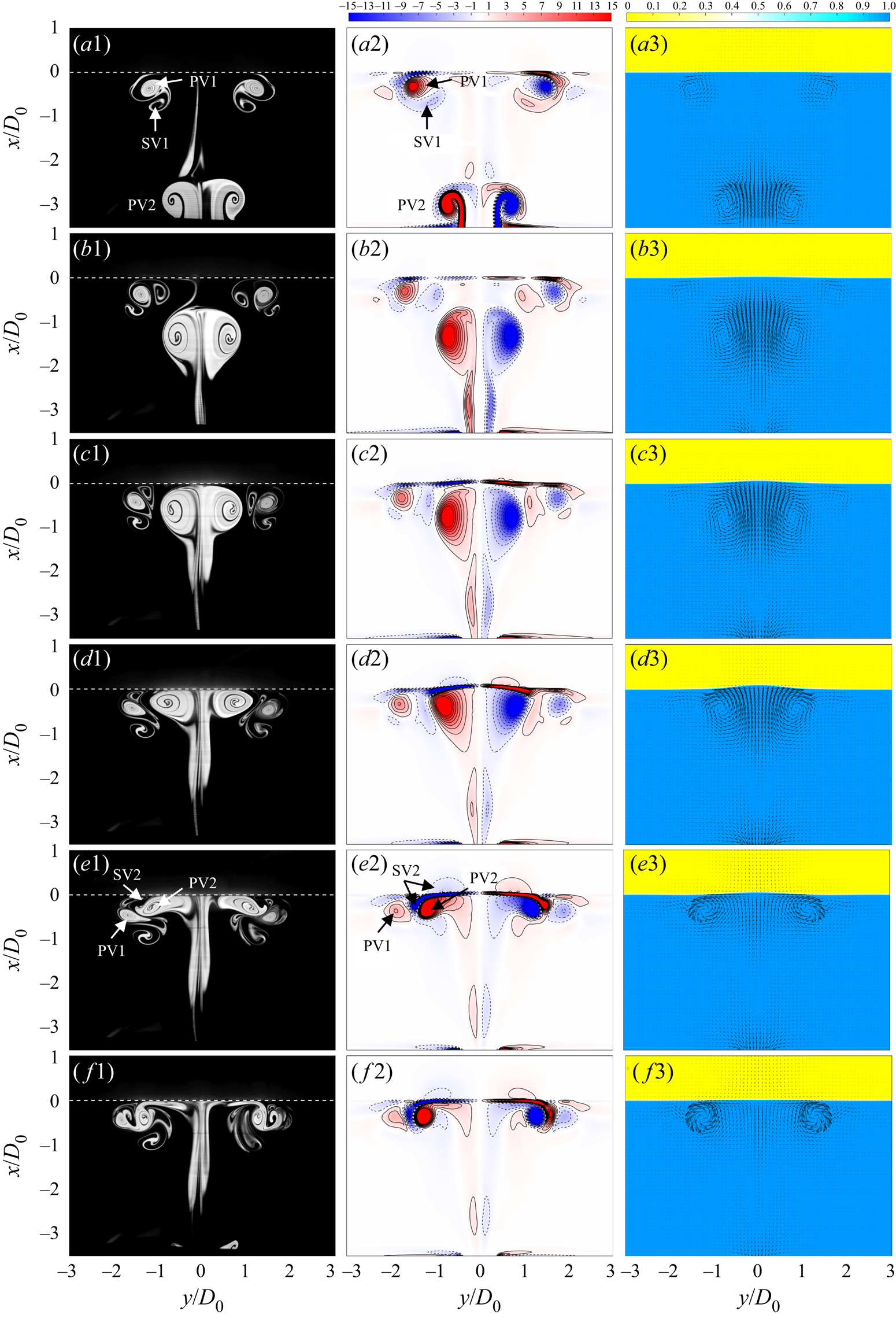
Figure 5. Temporal evolution of LIF flow visualization (first column), spanwise vorticity  ${\omega _z}{D_0}/{U_0}$ (second column) and water volume fraction
  ${\phi _w}$ (third column) for the laminar case at t/T = 0.3 (a1–a3), 0.6 (b1–b3), 0.7 (c1–c3), 0.8 (d1–d3), 0.9 (e1–e3) and 1.0 ( f1–f3). PV denotes primary vortex ring, SV denotes secondary vortex ring in each phase fluid, and 1 and 2 denote vortical structures during two successive cycles. The white dashed line denotes the initial interface location of x/D 0 = 0.

Figure 6. Temporal evolution of LIF flow visualization (first column), spanwise vorticity  ${\omega _z}{D_0}/{U_0}$ (second column) and water volume fraction
  ${\phi _w}$ (third column) for the transitional case at t/T = 0.3 (a1–a3), 0.6 (b1–b3), 0.8 (c1–c3) and 1.0 (d1–d3).
For the laminar case, after impingement of the primary vortex ring (PV1) on the interface, the formation of the secondary vortex ring (SV1) in water is clearly observed, which is orbiting the PV1 towards the jet centreline (figure 5a1,a2). As the new primary vortex ring (PV2) moves upwards and collides with the interface, the core of the PV2 gradually flattens and SV1 is severely squeezed between the PV1 and PV2 (figure 5d1,d2). In addition, the new secondary vortex ring (SV2) with opposite sense to the cores of the PV2 is induced in both water and oil layers, respectively (figure 5e2). These vortices are generated by baroclinic torque associated with variations in vertical pressure and horizontal density gradients caused by the vortex impinging on the density interface, as suggested by Advaith et al. (Reference Advaith, Manu, Tinaikar, Chetia and Basu2017). With radial stretching of the PV2, the SV2 in water continues to orbit the PV2 as described above, while the SV2 in oil gradually decays (figure 5f1, f2). As reflected by the water volume fraction, the density interface displays relatively small deformation during the vortex impingement due to a lower jet velocity. Thus, the vortical structure evolution is less affected by the interface deformation so that the overall flow patterns resemble those for the vortex ring impinging on solid boundaries (Orlandi & Verzicco Reference Orlandi and Verzicco1993; Cheng et al. Reference Cheng, Lou and Luo2010; Xu et al. Reference Xu, He, Kulkarni and Wang2017).
The transitional case displays significant differences in the vortex–interface interaction and the interface deformation compared with the laminar case. With increasing Reynolds number, the primary vortex ring could rapidly lose its symmetry about the jet centreline during the convection, and small-scale vortices are formed in the wake as a consequence of the Kelvin–Helmholtz instability in the shear layer (figure 6b1). As the PV2 collides with the density interface, segments of the PV2 have crossed the initial interface location, which severely deform the interface to be a dome-like shape (figure 6c1–c3). The strong vortex–interface interaction, in turn, results in more flattened cores of the PV2 along the normal direction of the deforming interface. The formation of the SV2 is also detected, especially for the numerical result (figure 6c2), which could effectively capture the SV2 in oil despite a larger deformation of the interface. During radial stretching of the PV2, the SV2 in water seems to be broken up due to intense vortical interactions, while the SV2 in oil has greater scale and strength than that for the laminar case (figure 6d2). The interfacial waves caused by strong impingement of the vortex rings can continuously propagate outward owing to the presence of a restoring buoyancy force (figure 6d3). It is also noted that the interface behaviours for the laminar and transitional cases identified in this study can match the no-rebounding and rebounding regimes of Song et al. (Reference Song, Choi and Kim2021) for an isolated vortex ring interaction with the water–oil interface.
However, the present study focuses on the converged results of successive vortex rings impinging on the interface, which display some differences from an isolated situation. For a comparison, figure 7 presents the LIF flow visualization in the first jet cycle for the laminar and transitional cases which could represent approximately an isolated vortex ring impinging on the interface. As shown in figure 7(a–c), the primary vortex ring in the first jet cycle for the laminar case displays similar behaviour to that in figure 5; however, complex interactions between different vortex rings are apparently absent for the isolated situation.

Figure 7. Evolution of LIF flow visualization in the first jet cycle for the laminar (a–c) and transitional (d–f) cases at t/T = 0.4 (a,d), 0.7 (b,e) and 1.0 (c, f).
For the transitional case, the primary vortex ring in the first cycle convects with better symmetry about the jet centreline due to no pre-existing external perturbance. Subsequently, the primary vortex ring could shrink during its penetration into the oil layer, and eventually penetrate the interface almost completely, leading to a larger maximum height of the interface deformation (figure 7e). Soon after that, the primary vortex ring is detected to reverse its direction and return into the water layer with opposite rotational sense of the cores due to the buoyancy effect (figure 7f). However, such phenomenon has not happened to the corresponding case of successive vortex rings, and the relevant reasons can be explained here. The interface deformation during the vortex impingement essentially stems from the conversion of kinetic energy into potential energy. For successive vortex rings, there could be small-scale structures in front of the primary vortex ring before its collision with the interface due to strong vortex–interface interactions in previous cycles. The interaction of the primary vortex ring with these small scales could cause strength reduction and energy dissipation, however, that does not happen to an isolated case. As a result, less vortex kinetic energy is converted into potential energy of the interface for synthetic jets, leading to a lower maximum penetration height and no formation of an outstanding reversed jet from oil to water in comparison to the isolated case.
The dynamics of the vortical structure evolution is further quantitatively depicted in figure 8. The vortex centre is defined as the centroid of the vorticity (Cantwell & Coles Reference Cantwell and Coles1983) and is calculated as
 \begin{gather}{x_v} = \frac{1}{\varGamma }\int_\varOmega {x{\omega _z}\,\textrm{d}\varOmega } ,\end{gather}
 \begin{gather}{y_v} = \frac{1}{\varGamma }\int_\varOmega {y{\omega _z}\,\textrm{d}\varOmega } ,\end{gather}
 \begin{gather}\varGamma = \int_\varOmega {{\omega _z}\,\textrm{d}\varOmega } ,\end{gather}
where  $\varOmega $ denotes the vortex region determined by the
  ${\lambda _{ci}}$ criterion (Zhou et al. Reference Zhou, Adrian, Balachandar and Kendall1999). In this study, the flow area with a
  ${\lambda _{ci}}$ above 0.5 s−1 is recognized as the vortex area. This threshold could effectively distinguish the vortex ring from the shear layer while retaining most of the vorticity, and the results are also insensitive to this cut-off level. Within this vortex area, the entire vorticity is used for the above integrations. Note, during the primary vortex ring interaction with the interface, the secondary vortex ring in the last cycle (SV1) is relatively weak and difficult to be identified by the
  ${\lambda _{ci}}$. Hence, only the circulation of the SV2 including those in both water and oil layers is calculated.

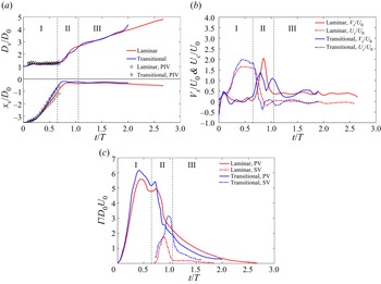
Figure 8. Temporal evolution of (a) primary vortex ring diameter Dv/D 0 and streamwise trajectory xv/D 0, (b) stretching velocity Vs/U 0 and convective velocity Uc/U 0, and (c) core circulation  $\varGamma/D_{0}U_{0}$ of the primary vortex ring and secondary vortex ring for the laminar and transitional cases.
The vortex ring diameter equals the distance between vortex centres corresponding to the positive and negative vorticities. Based on changes in the growth rate of the vortex ring diameter, the process of the vortex ring impinging on the interface can be divided into three stages, i.e. vortex free-travel, vortex–interface interaction and vortex stretching stages, as marked by I, II and III in figure 8(a). In addition, the numerical results are compared with those from PIV in terms of the vortex diameter and streamwise trajectory before it collides with the interface. The simulations could reasonably reflect the vortical structure evolution of the experimental counterparts despite the local discrepancies in the streamwise trajectory for the laminar case, which could be due to different energy dissipations between the experiment and numerical simulation.
In the free-travel stage (stage I), the diameter of the formed primary vortex ring displays little change. The streamwise trajectory varies approximately linearly with the time, and the convection velocity produces a local platform after reaching the maximum value. Here, the vortex ring translational velocity Ut before impinging on the interface can be obtained by the linear fit of the vortex centre streamwise trajectory. The resultant translational velocity is 33.83 and 80.53 mm s−1 for the two cases corresponding to 1.58U 0 and 1.88U 0, respectively. Thus, the Froude number based on the vortex translational velocity Fr is computed as (Linden Reference Linden1973; Herault et al. Reference Herault, Facchini and Bars2018)
 \begin{equation}Fr = \frac{{U_{t}}}{{\sqrt {g^{\prime}{D_0}} }},\end{equation}
where  $g^{\prime}( = g\Delta \rho /{\rho _w})$ is the reduced gravitational acceleration. Consequently, Fr is 0.35 and 0.82 for the two cases. In addition, the circulation of the primary vortex ring also increases approximately linearly during the translation, and reaches a larger peak value for the transitional case than the laminar case.
As the primary vortex ring enters stage II, a significant increase in the vortex ring diameter and stretching velocity is detected, indicating the onset of the vortex–interface interaction. Such behaviour is associated with the retardation of the vortex ring when it encounters strong resistance due to buoyancy, and thus leads to stretching of the vortex diameter. Meanwhile, a local increase in the circulation occurs for the two cases due to local compression of the vortex core. Once the secondary vorticity is baroclinically generated near the interface, the circulation of the primary vortex ring decreases dramatically and the transitional case exhibits a larger decay rate than the laminar case due to the influence of stronger baroclinic vorticity. In the later period of stage II, the circulation of the secondary vortex ring decreases rapidly for the two cases with the interface recovery due to buoyancy.
The influence of the vortex–interface interaction on the vortex ring circulation is further discussed here. In this study, when an initially stably stratified system (light fluid above dense fluid) is perturbed by the vortex impingement, misalignment in pressure and density gradients is created due to dense fluid above light fluid, as shown in figure 9. According to vorticity-transportation equation in a variable density flow (Advaith et al. Reference Advaith, Manu, Tinaikar, Chetia and Basu2017):
 \begin{equation}\frac{{\textrm{D}\boldsymbol{\omega }}}{{\textrm{D}t}} = \boldsymbol{\omega }\boldsymbol{\cdot }\boldsymbol{\nabla }\boldsymbol{u} + \nu {\nabla ^2}\boldsymbol{\omega } + \frac{1}{{{\rho ^2}}}(\boldsymbol{\nabla }\rho \times \boldsymbol{\nabla }p),\end{equation}
the last term depicts baroclinic torque and can be written as  $(1/{\rho ^2})((\partial \rho /\partial y)(\partial p/\partial x) - ((\partial \rho /\partial x)(\partial p/\partial y))$ in a two-dimensional case, thus leading to the generation of opposite sign vorticity to that of the primary vortex ring. As a result, the vorticity cancellation occurs along the edge of the induced boundary layer due to the interaction between the primary vortex ring and baroclinic vorticity, and that is believed to be the major cause for the circulation reduction of the primary vortex ring during the vortex–interface interaction (Chu et al. Reference Chu, Wang and Hsieh1993). In addition, another possible mechanism of impacting the circulation is that part of the kinetic energy of the primary vortex ring can be dispersed by the fast-propagating interfacial waves caused by the vortex impingement. The total kinetic energy of the vortex motion is proportional to the circulation (Kambe & Mya Oo Reference Kambe and Mya Oo1984), and thus the circulation of the primary vortex ring could also be reduced.

Figure 9. Schematic of the baroclinic generation of vorticity during the vortex–interface interaction.
In the last stage (stage III), the vortex ring diameter increases with a lower growth rate relative to stage II, which somewhat resembles that of Song et al. (Reference Song, Bernal and Tryggvason1992) for an isolated vortex ring impinging on the free surface at higher Froude number (Fr = 0.988). The primary vortex ring for the laminar case undergoes stretching with a relatively constant velocity owing to recovery of the interface. However, evident fluctuations of the stretching and convective velocities can still be detected for the transitional case, suggesting consecutive interactions between vortex rings and the interface. Additionally, the circulations of the primary and secondary vortex rings gradually decay, which is mainly attributed to the viscous effect. The present results characterize the dynamics of successive vortex rings impinging on the stratified interface. Although there is much difference in the Reynolds number and Froude number for the two cases, the behaviour of the primary vortex ring could follow a similar evolution process.
Figure 10 displays the evolution of three-dimensional vortical structures for the laminar case based on the vorticity iso-surface  $|{\omega _{xyz}}|{D_0}/{U_0}(|{\omega _{xyz}}|= \sqrt {\omega _x^2 + \; \omega _y^2 + \; \omega _z^2} )$ from different views. Note that the vorticity iso-surfaces of two different thresholds are examined. The lower vorticity iso-surface is coloured by the streamwise vorticity
  $\omega_{x}{D_0}/{U_0}$ and water volume fraction
  ${\phi _w}$, as shown by the legend. They are used to identify the hairpin vortex or streamwise vortex, and thus to reveal the vortical structure evolution in both water and oil phases. The higher vorticity iso-surface is coloured by green to reflect the interaction between the primary vortex ring and other vortical structures. In addition, figure 11 provides the evolution of local three-dimensional vortical structures to clearly illustrate the formation and evolution of the hairpin vortex and complex interaction with the primary vortex ring.

Figure 10. Evolution of 3-D vorticity iso-surface  $|{\omega _{xyz}}|{D_0}/{U_0} = 2.5$ coloured by the streamwise vorticity
  ${\omega _x}{D_0}/{U_0}(|{\omega _{xyz}}|{D_0}/{U_0} = 10$ coloured by green is displayed together, first column) and water volume fraction
  ${\phi _w}$ (second column) for the laminar case at t/T = 0.3 (a1,a2), 0.6 (b1,b2), 0.8 (c1,c2) and 1.0 (d1,d2). The first column represents upward view and the second column represents downward view.

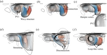
Figure 11. Evolution of local 3-D vorticity iso-surface in figure 10 at t/T = 0.3 (a), 0.45 (b), 0.6 (c), 0.75 (d) 0.85 (e) and 1.0 ( f).
It is noticed that extreme azimuthal waviness has been developed at the cores of the SV1 in water when it orbits into the interior of the PV1, and the corresponding wavenumber m equals 8 (see figure 10a1). The development of a certain amount of azimuthal wave on the vortex ring surface is due to the azimuthal instability (Widnall, Bliss & Tsai Reference Widnall, Bliss and Tsai1974; Morre & Saffman Reference Morre and Saffman1975), which has been well known in studies of a vortex ring interaction with the free-slip (Dahm et al. Reference Dahm, Scheil and Tryggvason1989; Archer et al. Reference Archer, Thomas and Coleman2010; Olsthoorn & Dalziel Reference Olsthoorn and Dalziel2017) and no-slip (Walker et al. Reference Walker, Smith, Cerra and Doligalski1987; Orlandi & Verzicco Reference Orlandi and Verzicco1993; Ren & Lu Reference Ren and Lu2015) boundaries. The present study further validates that it also exists in the interaction of vortex rings with the immiscible interface.
Subsequently, the wavy structure of the SV1 in water undergoes disconnection of the vortex core closer to the interface under the self-induction effect, followed by the formation of the hairpin vortex which attaches to the interface through a reconnection process (see figure 11a,b). As the PV2 approaches and collides with the interface, the formation of the SV2 in oil can be observed in figure 10(c2). Meanwhile, complex interaction between the PV2 and the formed hairpin vortices is further detected in figures 10(c1,d1) and 11(c–f). To facilitate the understanding, the main interaction process has been depicted by the schematic models in figure 12 in the form of a single hairpin vortex interaction with the primary vortex ring.

Figure 12. Schematic models for illustrating the interaction between the primary vortex ring and hairpin vortex at three phases. Different vortical structures are displayed by blue, green and red patterns. The black arrow in panel (a) denotes local rotation sense of vortices.
An inverted hairpin vortex can be observed in figure 11(c) with the legs attaching to the interface, and the head of the hairpin vortex has the opposite rotation sense to that of the primary vortex ring (figure 12a). Subsequently, the hairpin vortex could be stretched along the PV2 surface with the head tending to be entrained by the PV2 (figures 11d and 12b). With radial stretching of the PV2, the deformed hairpin vortex further undergoes the core disconnection at the head (see figure 11e), and eventually evolves into a series of loop-like vortices wrapping the PV2 (figures 11f and 12c). These loop-like vortices are products of successive vortex–interface interactions, which have not been mentioned in the previous studies of an isolated vortex ring impinging on the interface. The present results can provide more meaningful details of the evolution and deformation of the hairpin vortex as well as its interaction with the primary vortex ring in an axisymmetric flow, highlighting the significance of 3-D numerical simulation.
For the transitional case in figure 13, the flow field becomes significantly three-dimensional with a great number of different-scale structures caused by intense interactions between vortex rings and the interface, and different vortical structures. With increasing Reynolds number, the primary vortex ring rapidly develops azimuthal deformation in its convection toward the interface, so that streamwise vortices are formed by wrapping the vortex cores and then remain in the jet wake (figure 13c1). During the vortex–interface interaction, strong secondary vortices are induced in both water and oil layers. The SV2 in oil is clearly shown in figure 13(c2,d2) as a large-scale coherent structure; however, the SV2 in water rapidly develops vortex breakdown due to strong interaction with the PV2, resulting in a series of hairpin vortices wrapping the PV2 (see the zoom-in image in figure 13d1). In addition, it is noticed that the secondary vortices induced at the interface location move radially (figure 13d2,a2), suggesting outward propagation of the interfacial waves caused by strong vortex impingement. Such flow patterns can also verify that partial kinetic energy of the primary vortex ring is dispersed by the fast-propagating interfacial waves for the transitional case.

Figure 13. Evolution of 3-D vorticity iso-surface  $|{\omega _{xyz}}|{D_0}/{U_0} = 2.5$ coloured by the streamwise vorticity
  ${\omega _x}{D_0}/{U_0}(|{\omega _{xyz}}|{D_0}/{U_0} = 10$ coloured by green is displayed together, first column) and water volume fraction
  ${\phi _w}$ (second column) for the transitional case at t/T = 0.3 (a1,a2), 0.6 (b1,b2), 0.8 (c1,c2) and 1.0 (d1,d2). An inverted view zooming in on the structures near the interface is shown on the left of panel (d1).
4.2. Vortex ring instability
This section will discuss the vortex ring instability during the evolution and interaction with the density interface. First, a coordinate transformation is performed to obtain the radial velocity ur and azimuthal velocity  $u_{\theta}$ in the cylinder coordinate system. Then the azimuthal vorticity
  $\omega_{\theta}$ could be computed as
  $\omega_{\theta} = \partial u/\partial r - \partial {u_r}/\partial x$. In the present 3-D numerical simulation, the wavy structures have been detected as a consequence of the secondary vortex ring subjected to the azimuthal instability. To quantitatively characterize the vortex ring instability, we perform an azimuthal Fourier decomposition of
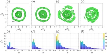
  ${\omega _\theta }$, which has been widely used to extract the flow quantity of each azimuthal mode in the instability analysis of the free vortex ring (Archer et al. Reference Archer, Thomas and Coleman2008), and single vortex–interface (Archer et al. Reference Archer, Thomas and Coleman2010; Olsthoorn & Dalziel Reference Olsthoorn and Dalziel2017) and vortex–wall (Ren & Lu Reference Ren and Lu2015) interactions.
Here we focus on the instability property of the primary vortex ring, whose structures can be extracted from the 3-D flow field corresponding to the threshold of  ${\omega _\theta } < 0$. In addition, a cylinder control volume fixed on the vortex centre of the primary vortex ring is used for the related integration within the streamwise, radial and azimuthal ranges of
  $[{x_v} - {D_0}/2,{x_v} + {D_0}/2]$,
  $[0,({R_{v1}} + \; {R_{v2}})/2]$ and
  $[0,2\mathrm{\pi }]$, respectively, where Rv 1 and Rv 2 denote radii of the PV1 and PV2. The vortex centre location and the ring radius can be obtained from figure 8, and this range is selected to remove the probable impact of the vortex ring from the previous jet cycle. In each
  $r{-}\theta $ plane, the azimuthal vorticity with the wavenumber m can be expressed as
 \begin{equation}{\omega _m} = {\xi _m}\cos (m\theta ) + {\zeta _m}\sin (m\theta ),\end{equation}
where  ${\xi _m} = (1/\mathrm{\pi })\int_0^{2\mathrm{\pi }} {{\omega _\theta }} \cos (m\theta )\,\textrm{d}\theta $ and
  ${\zeta _m} = (1/\mathrm{\pi })\int_0^{2\mathrm{\pi }} {{\omega _\theta }} \sin (m\theta )\,\textrm{d}\theta $. Then the amplitude of
  ${\omega _m}$ can be measured using Am as follows (Ren & Lu Reference Ren and Lu2015; Olsthoorn & Dalziel Reference Olsthoorn and Dalziel2017):
 \begin{equation}{A_m}(x,t)\; = \; \sqrt
{\displaystyle\frac{\displaystyle{\mathop \int_0^{2\mathrm{\pi }}
\mathop \int_0^{({R_{v1}} + \; {R_{v2}})/2}
{\omega _m}^2r\,\textrm{d}r\,\textrm{d}\theta }}{\displaystyle{\mathop
\int_0^{2\mathrm{\pi }} \mathop \int_0^{({R_{v1}} + \; {R_{v2}})/2}
r\,\textrm{d}r\,\textrm{d}\theta }}}
.\end{equation}
\begin{equation}{A_m}(x,t)\; = \; \sqrt
{\displaystyle\frac{\displaystyle{\mathop \int_0^{2\mathrm{\pi }}
\mathop \int_0^{({R_{v1}} + \; {R_{v2}})/2}
{\omega _m}^2r\,\textrm{d}r\,\textrm{d}\theta }}{\displaystyle{\mathop
\int_0^{2\mathrm{\pi }} \mathop \int_0^{({R_{v1}} + \; {R_{v2}})/2}
r\,\textrm{d}r\,\textrm{d}\theta }}}
.\end{equation}
The non-dimensional averaged amplitude of each azimuthal mode of the primary vortex ring is further calculated as
 \begin{equation}\overline {A_m^\ast (t)}
= \frac{\displaystyle{\int_{{x_v}\; - {D_0}/2}^{{x_v}\; + \; {D_0}/2}
{{A_m}(x,t)\,\textrm{d}x} }}{{{D_0}}} \times
\frac{{\displaystyle{D_0}}}{{{U_0}}} = \frac{\displaystyle{\int_{{x_v}\; -
{D_0}/2}^{{x_v}\; + \; {D_0}/2} {{A_m}(x,t)\,\textrm{d}x}
}}{{{U_0}}}.\end{equation}
\begin{equation}\overline {A_m^\ast (t)}
= \frac{\displaystyle{\int_{{x_v}\; - {D_0}/2}^{{x_v}\; + \; {D_0}/2}
{{A_m}(x,t)\,\textrm{d}x} }}{{{D_0}}} \times
\frac{{\displaystyle{D_0}}}{{{U_0}}} = \frac{\displaystyle{\int_{{x_v}\; -
{D_0}/2}^{{x_v}\; + \; {D_0}/2} {{A_m}(x,t)\,\textrm{d}x}
}}{{{U_0}}}.\end{equation}
To analyse the azimuthal variations of the primary vortex ring, figure 14(a–d) displays the iso-surface of  ${\omega _\theta }{D_0}/{U_0} ={-} 3$ at several selected moments through the three evolution stages for the laminar case. The PV2 displays an axisymmetric distribution at t/T = 0.6 before impinging on the interface. As the PV2 collides with the interface and stretches radially, the PV2 gradually develops the azimuthal instability with the appearance of waviness at the vortex core from t/T = 0.85 to 1.3. Particularly, a phase difference can be observed for the azimuthal locations of the crest and trough between figures 14(c) and 14(d), indicating an obvious axial flow (circumferential flow along the vortex core axis). The axial flow can reflect appreciable azimuthal deformation of the vortex ring according to Naitoh et al. (Reference Naitoh, Fukuda, Gotoh, Yamada and Nakajima2002).

Figure 14. Iso-surface of azimuthal vorticity  ${\omega _\theta }{D_0}/{U_0} ={-} 3$ (a–d) and corresponding averaged amplitude
  $\overline {A_m^\ast} $ of the first 30 modes of the primary vortex ring (e–h) for the laminar case at t/T = 0.6 (a,e), 0.85 (b, f), 1.1 (c,g) and 1.3 (d,h).
The averaged amplitude  $\overline {A_m^\ast} $ of the first 30 azimuthal modes of the primary vortex ring is presented in figure 14(e–h). With the development of waviness at the vortex core, the wavenumber m = 8 displays the most profound peak in the spectrum as the dominant azimuthal mode. For a Gaussian core distribution of vorticity, the most amplified azimuthal mode depends on the slenderness ratio such that
  $m\sim 2.26/\varepsilon $ (Shariff et al. Reference Shariff, Verzicco and Orlandi1994), where
  $\varepsilon $ denotes the ratio of the vortex core radius and the vortex ring radius. For the laminar case,
  $\varepsilon $ is approximately 0.28 during the primary vortex ring translation before impinging on the interface, and thus leads to the theoretical prediction of the unstable wavenumber of m = 8, consistent with the numerical result.
In addition, it is noted that there is a local peak corresponding to the azimuthal mode m = 4 in each spectrum. This wavenumber is naturally generated by the grid-induced instability when simulating a circular vortex ring in Cartesian coordinates, which has been observed in previous numerical works (Verzicco & Orlandi Reference Verzicco and Orlandi1996; Stock, Dahm & Tryggvason Reference Stock, Dahm and Tryggvason2008; Cheng et al. Reference Cheng, Lou and Luo2010). According to the work of Cheng et al. (Reference Cheng, Lou and Luo2010), the impact of this numerical perturbation on the large-scale flow structures is far weaker than the artificial perturbation at low Reynolds number, and thus could be negligible. The present numerical simulation is performed at a comparable Reynolds number with that in Cheng et al. (Reference Cheng, Lou and Luo2010). Furthermore, the mode m = 4 has an apparently lower maximum than the dominant mode during the development of the vortex ring instability, and therefore will not interfere the determination of the dominant mode.
The azimuthal vorticity iso-surface and the corresponding averaged amplitude for the transitional case are presented in figure 15. It is worth noting that the PV2 displays an approximately triangular distribution at t/T = 0.6 before impinging on the interface, distinguished from that for the laminar case. With the PV2 interaction with the interface, the entire flow structures develop azimuthal deformation with the unstable wavenumber m = 3 at t/T = 0.9, and the corresponding amplitude grows significantly as the dominant mode. The dominant mode m = 3 can also be reflected by the azimuthal distribution of hairpin vortices in figure 9(d1), similar to that of Deng et al. (Reference Deng, Xue, Mao and Caulfield2017) for interacting vortex rings induced by an oscillating disk. In addition, a profound peak has also been detected for the mode m = 1 in figure 15(g). However, these low-order modes display differences from the linear theoretical prediction of the amplified azimuthal mode of m = 6 based on the slenderness ratio  $\varepsilon $ of approximately 0.37, which can be explained as follows.

Figure 15. Iso-surface of azimuthal vorticity  ${\omega _\theta }{D_0}/{U_0} ={-} 3$ (a–d) and corresponding averaged amplitude
  $\overline {A_m^\ast} $ of the first 30 modes of the primary vortex ring (e–h) for the transitional case at t/T = 0.6 (a,e), 0.74 (b, f), 0.9 (c,g) and 1.14 (d,h).
For the transitional case at a high Reynolds number, the initial vortex ring could be strongly affected by the perturbed flow field caused by the previous vortical structures. As a result, the vortex ring immediately becomes unstable and the linear axisymmetric mode is destroyed by nonlinear effects (see figure 6a1). Another nonlinear phenomenon is the development of the vortical structures on the periphery of the ring, leading to ejection of vorticity into the wake (see figure 13b1,c1). Due to nonlinear interaction of the modes at a certain amplitude, the low-order modes can develop greatly as the intermodulation product and surpass the linear and high-order modes before the transition to turbulence (Shariff et al. Reference Shariff, Verzicco and Orlandi1994; Dazin, Dupont & Stanislas Reference Dazin, Dupont and Stanislas2006; Archer et al. Reference Archer, Thomas and Coleman2008). Furthermore, the most amplified azimuthal mode m = 3 could also be found in Brancher, Chomaz & Huerre (Reference Brancher, Chomaz and Huerre1994) for the periodic vortex rings in round jets through adding the random fluctuations to the initial conditions. They observed the breakdown of axisymmetry, accompanied by the occurrence of strong streamwise vortex pairs in the braid region between consecutive vortex rings. The present vortical evolution displays similar features to those in Brancher et al. (Reference Brancher, Chomaz and Huerre1994).
To further reveal the influence of the vortex–interface interaction on the vortex ring instability, the non-dimensional averaged modal energy  $\overline {E_m^\ast} $ of the primary vortex ring is calculated as
 \begin{gather}{E_m}(x,t)\; = \; \frac{\displaystyle{\int_0^{2\mathrm{\pi }} {\int_0^{({R_{v1}} + \; {R_{v2}})/2}{\displaystyle\frac{1}{2}(u_{xm}^2 + u_{rm}^2 + u_{\theta m}^2)r\,\textrm{d}r\,\textrm{d}\theta } } }}{{\displaystyle\int_0^{2\mathrm{\pi }} {\int_0^{({R_{v1}} + \; {R_{v2}})/2} {r\,\textrm{d}r\,\textrm{d}\theta } } }},\end{gather}
 \begin{gather}\overline {E_m^\ast (t)} = \frac{\displaystyle{\int_{{x_v} - {D_0}/2}^{{x_v} + {D_0}/2} {{E_m}(x,t)\,\textrm{d}x} }}{\displaystyle{\frac{1}{2}U_0^2{D_0}}}, \end{gather}
where uxm, urm and  ${u_{\theta m}}$ respectively denote the streamwise, radial and azimuthal velocities of the mode m obtained by performing the azimuthal Fourier decomposition with (4.6). Figure 16 presents the temporal evolution of the selected averaged modal energies for the two cases.

Figure 16. Temporal evolution of selected averaged modal energy  $\overline {E_m^\ast} $ of the primary vortex ring for the laminar (a) and transitional (b) cases. The dashed lines correspond to the moments for dividing the three evolution stages.
For the laminar case, the energies of the dominant mode m = 8 and its higher harmonic m = 16 increase exponentially after the primary vortex ring starts to interact with the interface, and nearly reach the maximum by the end of the interaction stage. These results clearly indicate that the stratification can promote an earlier growth of the vortex ring instability since the azimuthal instability has not been observed in such a streamwise range for a free axisymmetric synthetic jet vortex ring at a comparable Reynolds number (Wang et al. Reference Wang, Feng and Xu2019). A similar phenomenon has also been observed by Olsthoorn & Dalziel (Reference Olsthoorn and Dalziel2017) for a single vortex ring interacting with the stratified interface. The mechanism of the stratification-enhanced instability could be attributed to the interaction between the primary vortex ring with hairpin vortices stemming from baroclinic vorticity. With stretching of the primary vortex ring, the modal energies decay due to the viscous effect at a low Reynolds number.
The results of the modes m = 1–6 are displayed for the transitional case. The mode m = 4 naturally generated by the grid-induced instability does not undergo a typical exponential growth despite a slightly increasing amplitude with the vortex–interface interaction. In contrast, the energies of other low-order modes have already increased obviously from the vortex free-travel stage due to nonlinear effects with increasing Reynolds number. Moreover, the mode m = 3 can reach the largest amplitude to be the dominant mode as expected. With the beginning of the vortex–interface interaction stage, the modal energies could continue to increase through a local platform, whereas decay earlier than those for the laminar case. These results suggest that for the transitional case, the effect of the Reynolds number seems to play a prior role in the growth of the vortex ring instability compared to the stratification. However, the instability may be modulated by the stratification through stronger vortex–interface interaction. That could be due to the energy transfer from the vortex ring to the outward-propagating interfacial waves, which will be discussed in the next section.
4.3. Spatio-temporal property of interface
This section will reveal the properties of the interface deformation and interfacial waves generated by the vortex ring impingement by studying the dynamics of the interface. In the stratified flow field, the relative density is defined as  ${\rho _{re}} = (\rho \; - {\rho _o})/(\rho_{w} - {\rho _o})$ varying between 0 and 1, and thus the instantaneous interface height h can be determined corresponding to the iso-density line of
  ${\rho _{re}} = 0.5$ (Herault et al. Reference Herault, Facchini and Bars2018).
Figure 17(a) presents the spanwise distribution of the interface height corresponding to the maximum interface deformation. It is shown that the maximum interface deformation exhibits a Guassian distribution under successive vortex–interface interactions. The maximum interface height produced by the transitional case could be six times larger than that for the laminar case, representing the maximum penetration depth hm of the vortex rings across the interface. According to Linden (Reference Linden1973), the balance between the vortex kinetic energy and the potential energy of the interface deformation can be given as
 \begin{equation}g\Delta \rho {h_m} = {\rho _w}U_{in}^2,\end{equation}
where Uin is the velocity of the vortex ring at the interface location of h = 0. Based on the assumption of Uin approximate to the vortex ring translational velocity Ut, the non-dimensional maximum penetration depth can be expressed as
 \begin{equation}\frac{{{h_m}}}{{{D_0}}}\sim \frac{{{\rho _w}U_t^2}}{{g\Delta \rho {D_0}}} = F{r^2}.\end{equation}
As shown in figure 17(b), the present numerical results for the two cases display good agreement with this relationship, indicating that the maximum penetration depth could be proportional to Fr 2 for successive vortex rings interacting with the interface, similar to the previous results for an isolated situation (Linden Reference Linden1973; Song et al. Reference Song, Choi and Kim2021).

Figure 17. (a) Spanwise profile of interface height h/D 0 corresponding to the maximum interface deformation for the two cases. The vertical coordinate scale is magnified four times relative to the horizontal one for clarity. (b) Maximum penetration depth hm/D 0 versus Fr 2 for the two cases.
The temporal behaviour of the interface height at different spanwise locations is presented in figure 18(a,b). The results clearly display the radial propagation of the interfacial waves caused by the vortex impingement on the interface. In particular, the wave for the laminar case can maintain a stable amplitude of the main component with a reduction in the local wavelet, while the wave amplitude for the transitional case suffers from a sharp attenuation with the increased spanwise location.

Figure 18. Temporal evolution of interface height h/D 0 (a,b) and power spectral density (PSD) of interface height perturbation h′ (c,d) at different spanwise locations for the laminar (a,c) and transitional (b,d) cases. Each PSD in panels (c,d) is shifted downward by 10−2 relative to the former one.
The interface height perturbation is further given as  $h^{\prime}(\kern-0.06em y,t) = h(\kern-0.06em y,t) - \bar{h}$, where
  $\bar{h}$ denotes the time-averaged interface height. Figure 18(c,d) displays the spanwise variations of power spectral density (PSD) of the interface height perturbation. Both the spectra exhibit the profound peaks corresponding to the dominant frequency fe and its higher harmonics, indicating that the propagation of the interfacial waves is controlled by the impingement of synthetic jet vortex rings. For the laminar case, many higher harmonics are still conspicuous at a further location of y/D 0 = 7. However, higher harmonics and even the dominant frequency become vague at this location for the transitional case, which can be attributed to the wave destabilization associated with the enhanced three-dimensionality of the interface deformation.
The three-dimensional deformation of the interface caused by the vortex impingement can be directly illustrated by the iso-surface of the interface height h/D 0 in the entire computational domain, as shown in figure 19. Note, the vertical scale has been magnified thirty times to clearly display the interface deformation at a further radial location. The distribution of the non-dimensional kinetic energy  $E_u^\ast = \rho ({u^2}\; + {v^2} + {w^2})/{\rho _w}U_0^2$ on the interface is presented simultaneously to measure the propagation characteristics of the interfacial waves. The laminar case is shown to produce a small protuberance with the height far less than the interface radial scale before the vortex–interface interaction (figure 19a1), indicating the influence of the vortex ring on the interface prior to the impingement. The distribution of kinetic energy resembles that of the primary vortex ring with the unstable mode m = 8 (figure 19a2). After the vortex ring impingement, the entire interface could remain relatively well axisymmetric with the outward propagation of ripples, and the kinetic energy mainly distributes in the central region.

Figure 19. 3-D iso-surface of interface height h/D 0 (first and third columns, the vertical coordinate scale is magnified thirty times for clarity) and corresponding distribution of kinetic energy  $E_u^\ast $ on the interface (second and fourth columns) for the laminar (first and second columns) and transitional (third and fourth columns) cases at t/T = 0.6 (a1–a4), 1.0 (b1–b4), 1.2 (c1–c4) and 1.4 (d1–d4).
In contrast, enhancement of the 3-D deformation of the interface can be detected for the transitional case. With the vortex ring approaching, the interface rises significantly and the depression outboard of the vortices is deeper (figure 19a3). It is found that the outside edge of the interface produces a wave-like deformation with a comparable long wavelength with the interface radial scale. After strong vortex–interface interaction, three local peaks are noted at the central protuberance (figure 19b3), and the interfacial waves as well as the depression propagate outward rapidly as reflected by the variations of the kinetic energy (figure 19b4). In particular, the kinetic energy displays an azimuthal distribution in a manner reminiscent of the unstable mode m = 3 of the primary vortex ring. With further interface deformation, the central region of the interface becomes a funnel shape due to the buoyancy effect (figure 19c3,d3), and the edge of the interface produces large-scale azimuthal deformation as a consequence of consecutive propagation of the interfacial waves. Therefore, it is reasonable to establish a connection between the outer interfacial destabilization and the vortex ring instability through the vortex–interface interaction.
To reveal the underlying relationship between the vortex ring instability and the interface dynamics, the 3-D velocity field on the interface is extracted to perform the azimuthal Fourier decomposition, and the modal energy is further computed as (4.9) and (4.10). Figure 20 examines the spatio-temporal properties of the selected modal energies. For the laminar case, the dominant mode m = 8 displays a larger amplitude only at the locations of r/D 0 = 1 and 2, and both the lower mode m = 1 and higher harmonic mode m = 16 have a lower amplitude throughout the investigated range. Additionally, the mode m = 4 generated by the grid-induced instability is observed to slightly move outward from r/D 0 = 3 to 5, whereas the energy amplitude is relatively low and decreases with the increased radial location.

Figure 20. Temporal evolution of selected modal energy  $E_m^\ast $ on the interface at radial locations of r/D 0 = 1 to 5 for the laminar (a) and transitional (b) cases. The dashed lines correspond to the moments for dividing the three evolution stages.
The transitional case shows a completely different behaviour. The initial amplitude of the dominant mode m = 3 is lower than that of m = 1 produced by nonlinear interaction of the modes; however, their energy amplitudes become comparable at r/D 0 = 2 and 3. Particularly, the energies of these characteristic modes, even the lower mode m = 2, can continuously move radially outwards, consistent with the kinetic energy distribution in figure 19. As the radial location further increases, the interface flow field is gradually completely dominated by m = 1, and an increase in the corresponding amplitude can also be observed from r/D 0 = 4 to 5. The above results can provide compelling evidence that under strong vortex–interface interaction, the perturbances corresponding to the unstable modes of the primary vortex ring can radially propagate on the interface, eventually leading to destabilization of outer interfacial waves. Based on the above analysis, the present study has established a profound connection between the dynamics of the vortex and the interface, which can elucidate the underlying mechanism of the interfacial deformation and destabilization caused by successive vortex–interface interactions.
5. Conclusions
In this paper, we conduct a study on the interaction of synthetic jet vortex rings with a stratified water–oil interface by the LIF flow visualization, 2-D PIV and 3-D numerical simulation. Two cases with vortex ring Reynolds number in the laminar and transitional regimes are analysed in detail, corresponding to the Froude number based on the vortex translational velocity Fr = 0.35 and 0.82, respectively.
Despite a large difference in the Reynolds number and Froude number, the vortex rings for the two cases are detected with a similar evolution that can be divided into three stages based on the vortex diameter growth rate, including vortex free-travel, vortex–interface interaction and vortex stretching. As products of the vortex–interface interaction, the secondary vortex rings are baroclinically generated in both water and oil, resulting in a sharp decrease in the primary vortex ring circulation. Particularly, the transitional case produces a larger decay rate due to stronger baroclinic vorticity as well as energy dispersion by the fast-propagating interfacial waves. In addition, the vortical interaction triggers azimuthal waviness at cores of the secondary vortex ring in water, followed by the formation of hairpin vortices with legs attaching on the interface, and loop-like vortices wrapping the primary vortex ring. The present results can help to better understand the complex dynamics of successive vortex–interface interactions.
The azimuthal Fourier decomposition is used to analyse the vortex ring instability so as to reveal the influence of the vortex–interface interaction. The laminar case develops the most amplified unstable mode m = 8, consistent with the linear theoretical predict. The growth of the modal energy in the vortex–interface interaction stage indicates that the vortex ring instability is enhanced by the stratification, which is associated with the primary vortex ring interaction with hairpin vortices. However, increasing the Reynolds number has an impact on the vortex ring instability prior to the stratification. As a consequence, the transitional case develops an unstable mode m = 3 as well as other low-order modes from the vortex free-travel stage due to nonlinear interaction of the modes before the transition to turbulence.
The spatio-temporal properties of the interface are further revealed by analysing the dynamics of the interface. It is found that the maximum penetration height of vortex rings for the two cases is proportional to Fr 2, similar to that for an isolated situation. The radial propagation of the interfacial waves is dominated by the vortex impingement. Particulary, the transitional case produces destabilization of the interfacial waves at a further radial location with enhancement of the three-dimensional deformation of the interface. The instability analysis of the flow field on the interface demonstrates that the interfacial destabilization can be attributed to the radial propagation of perturbances stemming from the vortex ring instability through strong vortex–interface interaction. This significant finding could shed light on the mechanism of the interface deformation and destabilization, which has been mostly ignored in the previous studies. The present work can help to understand the fundamental mechanism. More investigations over a large range of control parameters, especially for turbulent synthetic jet vortex rings, should be performed to obtain a full regime map of successive vortex–interface interactions.
Acknowledgements
The authors gratefully acknowledge Dr D.T.H. New and Dr X. Mao for valuable comments regarding this work.
Funding
This work was supported by the National Natural Science Foundation of China (nos 11722215, 12102029 and 11721202), and the Postdoctoral Science Foundation Grant of China (no. 2021M690301).
Declaration of interests
The authors report no conflict of interest.