2.1. The FENE-P fluid equations

To characterise the rheology of dilute polymer solutions we use the FENE-P model proposed by Bird, Dotson & Johnson (Reference Bird, Dotson and Johnson1980). The momentum equation is given by

(2.1)\begin{equation} \frac{\partial \boldsymbol{u}}{\partial t} + \boldsymbol{u} \boldsymbol{\cdot} \boldsymbol{\nabla} \boldsymbol{u} ={-}\frac{1}{\rho}\boldsymbol{\nabla} p + \nu^{[s]} \nabla^{2} \boldsymbol{u} + \frac{1}{\rho} \boldsymbol{\nabla} \boldsymbol{\cdot} \boldsymbol{\sigma}^{[p]}, \end{equation}

where $\boldsymbol {u}$ is the velocity field, $\rho$ the solvent density, $p$ the pressure, $\nu ^{[s]}$ the (Newtonian) solvent kinematic viscosity and $\boldsymbol {\sigma }^{[p]}$ is the polymer stress tensor, which is calculated as

(2.2)\begin{equation} \boldsymbol{\mathsf{\sigma}}^{[p]} =\frac{\rho \nu^{[p]}}{\tau_p} [\, f(C_{kk}) \boldsymbol{\mathsf{C}} - \boldsymbol{\mathsf{I}}], \end{equation}

where $\nu ^{[p]}$ is the zero-shear-rate kinematic viscosity of the solution, $\tau _p$ is the maximum relaxation time of the polymer chains, $\boldsymbol{\mathsf{I}}$ is the identity matrix, $f(C_{kk}) \equiv (L^{2}-3)/(L^{2}-C_{kk})$ is the Peterlin function and $\boldsymbol{\mathsf{C}}$ is the conformation tensor. The model parameter $L^{2}$ is the square of the maximum extensibility of the polymer molecules normalised by their equilibrium radius $\langle R^{2} \rangle _0$ (the brackets denote an ensemble average over all configurations of the chain) and the conformation tensor is by definition the normalised covariance matrix of the polymer chain end-to-end vector $\boldsymbol {r}$, i.e. $\boldsymbol{\mathsf{C}} \equiv \langle \boldsymbol {r}'\boldsymbol {r}' \rangle /\langle R^{2} \rangle _0$. The conformation tensor $\boldsymbol{\mathsf{C}}$ is governed by the following evolution equation:

(2.3)\begin{equation} \frac{\partial \boldsymbol{\mathsf{C}}}{\partial t} +\boldsymbol{u} \boldsymbol{\cdot}\boldsymbol{\nabla} \boldsymbol{\mathsf{C}} = \boldsymbol{\nabla} \boldsymbol{u}^{\rm T} \boldsymbol{\cdot} \boldsymbol{\mathsf{C}} +\boldsymbol{\mathsf{C}} \boldsymbol{\cdot}\boldsymbol{\nabla} \boldsymbol{u} - \frac{1}{\tau_p} [f(C_{kk})\boldsymbol{\mathsf{C}}- \boldsymbol{\mathsf{I}}], \end{equation}

where the first two terms on the right-hand side of (2.3) represent the elongation of the polymer chains caused by the velocity gradients (polymer stretching/distortion term) and the last term represents the potential elastic energy stored in the polymers (relaxation term). Finally, the fluid incompressibility condition is imposed by the continuity equation

(2.4)\begin{equation} \boldsymbol{\nabla}\boldsymbol{\cdot} \boldsymbol{u}=0, \end{equation}

which closes the set of equations to be solved in the numerical simulations.

2.2. Numerical methods

In the present work the momentum equation is solved with a highly accurate code using pseudospectral/‘compact’ finite difference schemes, that has been used in several previous works (see da Silva, Lopes & Raman (Reference da Silva, Lopes and Raman2015), Guimarães et al. (Reference Guimarães, Pimentel, Pinho and da Silva2020) and references therein). The streamwise ($x$) derivatives are computed with a sixth-order ‘compact’ scheme (Lele Reference Lele1992) while the derivatives in the normal ($y$) and spanwise ($z$) directions are computed using pseudospectral methods (Canuto et al. Reference Canuto, Hussaini, Quarteroni and Zang1987), where dealiasing is performed with the $2/3$rd rule. Temporal advancement is computed with an explicit third-order low storage Runge–Kutta time-stepping scheme (Williamson Reference Williamson1980) and pressure–velocity coupling is ensured by a fractional step method (Kim & Moin Reference Kim and Moin1985).

Inflow and outflow boundary conditions are imposed in the boundaries facing the streamwise direction, with a prescribed inlet mean velocity profile superimposed to a random velocity fluctuation with an energy spectrum characteristic of isotropic turbulence, and non-reflective outflow boundary conditions at the outlet boundary (Orlanski Reference Orlanski1976).

The stretching term in the evolution equation of the conformation tensor field is calculated with central second-order finite differences, and the convection term is calculated with the shock-capturing scheme of Kurganov & Tadmor (Reference Kurganov and Tadmor2000). Cell area-averaged velocities are obtained as in Guimarães et al. (Reference Guimarães, Pimentel, Pinho and da Silva2020), while time advancement is performed with the same third-order explicit Runge–Kutta scheme used for the velocity update and no use is made of any artificial numerical diffusion. As in Guimarães et al. (Reference Guimarães, Pimentel, Pinho and da Silva2020), we monitored the values of the conformation tensor field for all points of the computational grid and checked that the symmetric positive-definiteness character of $\boldsymbol{\mathsf{C}}$ was maintained for all time iterations, as well as the six conditions imposed by the Cauchy–Schwartz inequality, e.g. $-\sqrt {|C_{11}^{\pm } C_{22}^{\pm }|} \leq C_{12}^{\pm } \leq \sqrt {|C_{11}^{\pm } C_{22}^{\pm }|}$.

In the present work we use the same numerical code employed in Guimarães et al. (Reference Guimarães, Pimentel, Pinho and da Silva2020) with a slight modification, for reasons of computational cost. In Guimarães et al. (Reference Guimarães, Pimentel, Pinho and da Silva2020) the method of Vaithianathan et al. (Reference Vaithianathan, Robert, Brasseur and Collins2006) is used to calculate the convection term of the conformation tensor equation, which can yield first- or second-order accuracy to the approximation of $\boldsymbol {u} \boldsymbol{\cdot}\boldsymbol {\nabla } \boldsymbol{\mathsf{C}}$, depending on which option maximises some eigenvalues of $\boldsymbol{\mathsf{C}}$ (see Guimarães et al. (Reference Guimarães, Pimentel, Pinho and da Silva2020) for details). This method is based on the work of Kurganov & Tadmor (Reference Kurganov and Tadmor2000) and it is designed to reduce the order of the approximation used in the computation of the convection term of the conformation tensor equation into first order, only at locations where shocks (discontinuities) arise in the conformation tensor field. The full version of the method requires the calculation of the eigenvalues of $54\times N_x \times N_y \times N_z$ three by three matrices at each Runge–Kutta time iteration, a number of order $O(10^{10})$ for the computational meshes used in the present study. Unlike as in Guimarães et al. (Reference Guimarães, Pimentel, Pinho and da Silva2020), in the present work the computation of the eigenvalues has been abandoned in order to reduce the computational costs, so that the approximation used in the computation of the convection term of the conformation tensor equation was fixed into first order. This leads to a speed-up of a factor of four in the present code and allows one to use extremely large domain sizes. Despite the lower order of this approximation compared with Guimarães et al. (Reference Guimarães, Pimentel, Pinho and da Silva2020), the computational meshes used in the present study remain considerably fine, of the order of one Kolmogorov microscale for all the viscoelastic cases at large $Wi$ (${\rm \Delta} x/\eta \approx 1$, see table 1) and thus the simplification has no impact on the conclusions of the work. This is shown in Appendix B, where one of the simulations used in the main text of the present work is repeated with the full second-order version of the method of Vaithianathan et al. (Reference Vaithianathan, Robert, Brasseur and Collins2006). Whereas the wake half-width and velocity deficit are virtually unchanged by the choice of the numerical method, the Reynolds stresses are slightly underestimated with the first-order method and the biggest ($i,j=1,1$) component of the conformation tensor shows the largest differences at the transition region of the flow, but follows the same qualitative trends everywhere else, i.e. in the fully developed turbulence region.

Table 1. Physical and computational parameters of the DNS of viscoelastic turbulent planar wakes: global/inlet Weissenberg number ($Wi=\tau _p {\rm \Delta} U_0/d$); polymer relaxation time ($\tau _p$); Taylor-based Reynolds number at the far-field region ($Re_\lambda$); spreading rate constant $A_{\delta }$; centreline velocity deficit decay rate $A_{{\rm \Delta} U}$; polymer stresses decay constant $A_{\sigma _c}$; polymer extension decay constant $A_{c_{ii}}$; grid spacing normalised by the Kolmogorov microscale at the middle of the computational domain ($y/d=0$ and $x/d=L_x/2d=42$) (${\rm \Delta} x/\eta _{42d}$).

2.3. Physical and computational parameters of the simulations

Table 1 lists the physical and computational parameters used in the simulations carried out in this work (viscoelastic numbers are defined later on). A total of five DNS were performed: four viscoelastic cases and one reference Newtonian case. The same uniform grid and computational domain sizes were used for all DNS, with $N_x=4032$, $N_y=1152$ and $N_z=288$ grid points in the streamwise ($x$), normal ($y$) and spanwise ($z$) directions, respectively, for a corresponding domain size of $L_x/d=84$, $L_y/d=24$ and $L_z/d=6$, where $d$ is the transverse length scale of the wake generator object. The results discussed in Appendix A confirm that the normal dimension of $L_y/d=24$ used here is sufficiently large to avoid undesirable confinement effects. To date the present DNS correspond to the largest simulations of turbulent viscoelastic FENE-P fluids in existence.

The Reynolds number based on the centreline velocity deficit at the inlet ${\rm \Delta} U_0$ was fixed at $Re_{{\rm \Delta} U}={\rm \Delta} U_0 d/\nu ^{[s]}=5000$, for all the simulations, which corresponds to a Reynolds number based on the free stream velocity $U_\infty$,

(2.5)\begin{equation} Re=\frac{U_\infty d}{\nu^{[s]}}, \end{equation}

approximately equal to $Re \approx 14\,286$, which is a definition more commonly used in studies of turbulent wakes originated at solid bodies. We define also a local Reynolds number based on the Taylor microscale $\lambda$,

(2.6)\begin{equation} Re_\lambda= \frac{\sqrt{\overline{u'^{2}}} \lambda}{\nu^{[s]}}, \end{equation}

where $\sqrt {\overline {u'^{2}}}$ is the root mean square (r.m.s.) velocity in the streamwise direction and the Taylor microscale $\lambda$ is calculated using the classical isotropic relation,

(2.7)\begin{equation} \lambda=\sqrt{\frac{15 \nu^{[s]}\overline{u'^{2}}}{\varepsilon^{[s]} } }, \end{equation}

with the mean viscous dissipation rate of the solvent given by

(2.8)\begin{equation} \varepsilon^{[s]} =2 \nu^{[s]} \overline{S_{ij}' S_{ij}'}, \end{equation}

where $S_{ij}' = ( \partial u_i' /\partial x_j + \partial u_j'/\partial x_i )/2$ is the fluctuating component of the rate-of-strain tensor. For the Newtonian (reference) simulation, the centreline $Re_\lambda$ approaches a constant value of $Re_\lambda \approx 100$ at the far field, which is approximately two times larger than in a recent experimental study on the self-similar character of cylinder wakes (Tang et al. Reference Tang, Antonia, Djenidi and Zhou2016). The mesh resolution is quantified by the ratio between the grid spacing ${\rm \Delta} x$ and the Kolmogorov microscale $\eta =(\nu ^{[s]^{3}}/\varepsilon ^{[s]})^{1/4}$. The values of ${\rm \Delta} x / \eta$ shown on table 1 were evaluated in the middle of the computational domain, i.e. at the centreline ($y/d=0$) and at $x/d=L_x/2d=42$.

For each time step the streamwise velocity $u(x,y,z,t)$ is prescribed at the inlet as the sum of a mean profile given by

(2.9)\begin{equation} \bar{u}(x=0,y) = U_\infty - \frac{{\rm \Delta} U_0}{2} \left\{1+ \tanh \left[ \frac{d}{4 \varPhi} \left( 1 - \frac{2|y|}{d} \right)\right]\right\}, \end{equation}

and a fluctuating component $u'(x,y,z,t)$, which is obtained from a pseudorandom number generator with the resulting fluctuating velocity exhibiting an energy spectrum $E(k)$ characteristic of isotropic turbulence, with an infrared region following a Batchelor spectrum, $E(k) \sim k^{4}$ ($k$ is the wavenumber vector in the $x,z$ inlet plane) and a prescribed peak wavenumber $k_p$ placed at the small scales of motion. This is done so that no relation with the ‘natural’ Kelvin–Helmholtz frequencies of the shear layer exists (Michalke Reference Michalke1965; Monkewitz & Huerre Reference Monkewitz and Huerre1982), which allows the momentum equations to ‘naturally select’ the natural instabilities of the flow. The initial inlet artificial noise is then ‘convoluted’ by a step function that prescribes it in the shear-layer region of the mean velocity profile (100 % of the generated fluctuations) and at the centre of the wake (25 % of the fluctuations). Before being imposed to the inlet velocity fluctuations, the instantaneous values of $u'(x,y,z,t)$ artificially generated are normalised to limit their maximum amplitude to $\text {max}|u'| = 0.15 U_\infty$. The entire procedure is very similar to the one described in detail in for example da Silva & Métais (Reference da Silva and Métais2002), and has no influence in the natural evolution of initial instabilities of the flow. The free stream velocity $U_\infty$ and the inlet mean velocity deficit ${\rm \Delta} U_0$ were set to $U_\infty = 1$ and ${\rm \Delta} U_0=0.35 U_\infty$, respectively, where the latter is close to the value obtained in the experiments of Liu, Thomas & Nelson (Reference Liu, Thomas and Nelson2002). The parameter $d/\varPhi$ in (2.9) dictates the value of the maximum mean velocity gradient at the inlet and it was fixed at $d/\varPhi =85$, giving ${\rm d} \bar {u}/{{\rm d}y} \sim 21.25 {\rm \Delta} U_0/d$ at the shear layer region of the profile. The normal and spanwise velocity components, $v(x,y,z,t)$ and $w(x,y,z,t)$, are treated similarly but have zero mean values, e.g. $v(x,y,z,t) = v'(x,y,z,t)$.

The inlet condition described above is similar to those used in Stanley & Sarkar (Reference Stanley and Sarkar1997) and da Silva et al. (Reference da Silva, Lopes and Raman2015) for simulations of turbulent jets and mixing layers and Hickey, Hussain & Wu (Reference Hickey, Hussain and Wu2013) and Zecchetto & da Silva (Reference Zecchetto and da Silva2021) for simulations of temporal wakes, but was adapted to the case of a spatially evolving turbulent wake. This method for simulating turbulent wakes with an imposed inlet velocity profile, instead of actually calculating the flow around the solid object, was probably used for the first time by Moser, Rogers & Ewing (Reference Moser, Rogers and Ewing1998) and has been shown to be a useful technique for studying the far-field regions of the flow with an acceptable computational cost.

In the literature of Newtonian turbulent wakes, the distance $x$ from the wake generator object is usually normalised either by the object transverse length scale $d$ or by the inlet momentum thickness $\theta (x=0)$, where $\theta$ is defined by

(2.10)\begin{equation} \theta=\int_{-\infty}^{\infty} \frac{\bar{u}}{U_\infty} \left( 1- \frac{\bar{u}}{U_\infty}\right){{\rm d}y}, \end{equation}

which is constant in the far field of a turbulent planar wake with a small velocity deficit. To simplify the notation, we use $\theta = \theta (x=0)$ so when reference is made to $\theta$ only the inlet value is being considered. We have reprocessed the data for turbulent planar wakes of Newtonian fluids from several works (Pot Reference Pot1979; Ramaprian Reference Ramaprian1984; Browne & Antonia Reference Browne and Antonia1986; Wygnanski, Champagne & Marasli Reference Wygnanski, Champagne and Marasli1986; Weygandt & Mehta Reference Weygandt and Mehta1989; Aronson & Löfdahl Reference Aronson and Löfdahl1993; Liu et al. Reference Liu, Thomas and Nelson2002; Tang et al. Reference Tang, Antonia, Djenidi and Zhou2016), as obtained behind solid objects with a variety of different geometries including splitter plates, circular cylinders, airfoils, solid strips and screens, and concluded that the scaling laws coefficients associated with the spreading rate of the wake $A_{\delta }$ and centreline velocity deficit decay rate $A_{{\rm \Delta} U}$ (see (3.1) and (3.2) below) cannot be made universal by either normalisation options, i.e. using either $d$ or $\theta$. However, when $d$ is used instead of $\theta$, the scatter in the values of these constants is considerably larger. This is particularly true for $A_{{\rm \Delta} U}$, which varies between $0.137 \leq A_{{\rm \Delta} U} \leq 2.91$ when $d$ is used as the normalisation parameter, and between $0.225 \leq A_{{\rm \Delta} U} \leq 0.411$ when $\theta$ is used instead. For this reason, and following Wygnanski et al. (Reference Wygnanski, Champagne and Marasli1986), we display our DNS results in coordinates of $x/\theta$ instead of $x/d$. The conversion between the two systems can be easily obtained for our data considering that the value of $d/\theta$ for all the simulations carried out in this work is $d/\theta =4.34$, for example the total extent of the domain in the streamwise direction is equal to $L_x/\theta = L_x/d \times d/\theta = 84 \times 4.34 \approx 365$ in all the simulations carried out in the present work.

For rheological parameters of the FENE-P model we use $L^{2}=100^{2}$ and $\beta = \nu ^{[s]} / (\nu ^{[s]} + \nu ^{[p]})=0.8$ in all the DNS carried out here, while $\tau _p$ is varied in order to simulate flows with different values of the global (or inlet) Weissenberg number $Wi$, which is defined by

(2.11)\begin{equation} Wi = \frac{\tau_p}{d/{\rm \Delta} U_0}. \end{equation}

Notice that a definition of $Wi$ based on the actual mean velocity gradient, instead of the velocity difference, would give values of $Wi$ that are $21.25$ times larger than those shown in table 1. We also define a local Weissenberg number $Wi_\eta (x)$ based on the ratio of the maximum relaxation time of the polymer molecules and the Kolmogorov time scale $\tau _\eta = (\nu ^{[s]} / \varepsilon ^{[s]} )^{1/2}$, which is computed at the centreline, i.e.

(2.12)\begin{equation} Wi_\eta(x) = \frac{\tau_p}{\tau_\eta}, \end{equation}

and a local Deborah number $De(x)$, which measures the influence of the fluid elasticity on the large scale energy-carrying eddies, here defined by

(2.13)\begin{equation} De(x)=\frac{\tau_p}{\delta(x)/{\rm \Delta} U(x)}, \end{equation}

where $\delta (x)$ is the half-width of the wake, defined in the classical way, i.e. ${\rm \Delta} \bar {u} (x,y=\delta )={\rm \Delta} U(x)/2$, where ${\rm \Delta} \bar {u}(x,y)= U_\infty - \bar {u}(x,y)$ is the mean velocity deficit, while ${\rm \Delta} U(x)={\rm \Delta} \bar {u}(x,y=0)$ is the local velocity deficit at the centreline. Notice that (2.13) contains the centreline velocity deficit instead of the mean velocity (as in the case of jets, e.g. Guimarães et al. (Reference Guimarães, Pimentel, Pinho and da Silva2020)) because the Deborah number definition is based on a flow time scale obtained from the mean velocity gradient, whose estimate is given by $\partial \bar {u}/\partial y \sim {\rm \Delta} U/\delta$. Also, notice that because the flow half-width at the inlet is $\delta (x=0) \approx d/2$ we obtain $De(x=0)\approx 2 Wi$ at this location, as confirmed below in § 3.2.

Finally, as in Ferreira et al. (Reference Ferreira, da Silva and Pinho2016), we define a solvent dissipation reduction parameter ($SDR$) evaluated at the centreline of the turbulent viscoelastic wake by

(2.14)\begin{equation} SDR(x)= \frac{\varepsilon^{[p]} }{ \varepsilon^{[p]} + \varepsilon^{[s]} }, \end{equation}

where $\varepsilon ^{[p]} = \overline {\boldsymbol {\sigma '}^{[p]} : \boldsymbol {\nabla } \boldsymbol {u}' }/\rho$ is the viscoelastic stress power and represents the flux of kinetic energy transported from the eddy motions into the fluid microstructure (and vice versa).

2.4. Validation

As described in Guimarães et al. (Reference Guimarães, Pimentel, Pinho and da Silva2020) and references therein, the present code has been used in several previous works where it has been thoroughly validated. In particular the work leading to that paper involved extensive validations in both laminar and turbulent jet configurations, using both Newtonian and viscoelastic (FENE-P) fluids. The solutions of the laminar cases were compared with the semianalytical solutions of the laminar viscoelastic jet recently derived by Parvar, da Silva & Pinho (Reference Parvar, da Silva and Pinho2020), while the turbulent solutions were extensively compared with statistics obtained in experimental and numerical results available in the literature. A similar approach has been used here for the reference turbulent Newtonian planar wake. Part of the extensive comparison is described in Appendix A in which the present results are compared with the experimental and numerical data from Townsend (Reference Townsend1949), Uberoi & Freymuth (Reference Uberoi and Freymuth1969), Narasimha & Prabhu (Reference Narasimha and Prabhu1972), Browne & Antonia (Reference Browne and Antonia1986), Wygnanski et al. (Reference Wygnanski, Champagne and Marasli1986), Weygandt & Mehta (Reference Weygandt and Mehta1989), Aronson & Löfdahl (Reference Aronson and Löfdahl1993), Zhou & Antonia (Reference Zhou and Antonia1995), Moser, Kim & Mansour (Reference Moser, Kim and Mansour1999), Schenck & Jovanovic (Reference Schenck and Jovanovic2002), Hickey et al. (Reference Hickey, Hussain and Wu2013) and Tang et al. (Reference Tang, Antonia, Djenidi and Zhou2016). The influence of the lateral ($L_y$) size of the computational domain was also investigated (see Appendix A) and showed that no undesired confinement effects exist in the very large simulations used here.

3.1. Contours of instantaneous vorticity magnitude

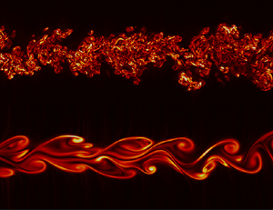
Figure 1 shows contours of instantaneous vorticity magnitude $|\boldsymbol {\omega }|$ for the DNS listed in table 1 with Weissenberg numbers equal to $Wi=1.1,2.1$ and $3.2$, together with the reference (Newtonian) case ($Wi=0$). Because the values of $|\boldsymbol {\omega }|$ decay in the streamwise direction $x$, different colormap ranges were used at different regions of the computational domain in order to properly visualise the flow. Furthermore, since $|\boldsymbol {\omega }|$ considerably decays when $Wi$ is increased, the colormaps range is also different for the different Weissenberg number cases. For example, the maximum $|\boldsymbol {\omega }|$ shown for the Newtonian case at the far field is $|\boldsymbol {\omega }|=10$, while we have set $|\boldsymbol {\omega }|=4$ for $Wi=3.2$. The case with $Wi=4.3$ is very similar to that with $Wi=3.2$ (not shown).

Figure 1. Contours of vorticity magnitude in the midplane ($z=0$) of the computational domain for turbulent planar wakes of viscoelastic fluids with different values of the Weissenberg number $Wi=1.1,2.1$ and $3.2$, together with the reference (Newtonian) case ($Wi=0$). Each simulation contains the entire domain (with $0 \le L_x/d \le 84$), however, different values of the vorticity magnitude threshold had to be used for each simulation in order to allow the visualisation of the flow in the entire computational domain (every subdomain using the same threshold is delimited by a vertical line). The figures do not show the total extent of the computational domain used in the lateral ($y$) dimension.

For the Newtonian wake ($Wi=0$ – figure 1a), Kelvin–Helmholtz instabilities arising in the upper and lower shear layers lead to the appearance of two rows of spanwise vortex rollers rotating in opposite directions – quasi-2-D Kármán vortices – and the formation of streamwise large vortex pairs due to the deformation of the primary vortices ($4 \lesssim x/d \lesssim 12$). Farther downstream, the flow structures are distorted by small-scale instabilities and by $x/d \gtrsim 25$ (or $x/\theta \gtrsim 100$) the flow becomes highly disorganised and with a broad range of eddy scales, characteristic of fully developed turbulence.

The results from the viscoelastic simulations are considerably different from the Newtonian case (figure 1b–d). Increasing the value of $Wi$ has a stabilising effect on the flow structures; the roll-up process of the shear layers appears to be delayed and there is a significant suppression of the small-scale vorticity, consistent with results obtained from earlier experiments (Cadot & Kumar Reference Cadot and Kumar2000; Cressman et al. Reference Cressman, Bailey and Goldburg2001), numerical simulations (Richter et al. Reference Richter, Iaccarino and Shaqfeh2012) and linear stability analyses (Azaiez & Homsy Reference Azaiez and Homsy1994; Richter, Shaqfeh & Iaccarino Reference Richter, Shaqfeh and Iaccarino2011). In particular, the vortex sheet structure for $Wi=2.1$ at $10 \lesssim x/d \lesssim 50$ (or $50 \lesssim x/\theta \lesssim 200$) is very similar to the structure observed in the soap film experiment of Xiong et al. (Reference Xiong, Bruneau and Kellay2013) with the highest polymer concentration, and for $x/d \gtrsim 60$ (or $x/\theta \gtrsim 250$) the roll-up of these vortex sheets leads to a structure which resembles the Newtonian case, but without much small-scale vorticity. Consistent with this, the next section shows that for $Wi=2.1$ the statistical quantities mainly associated with the large-scale structures, such as the first and second moments of the velocity field, are greatly modified by the presence of the polymers at $10 \lesssim x/d \lesssim 50$ but seem to recover a Newtonian appearance at $x/d \gtrsim 60$.

3.2. Classical statistics

Figure 2(a,b) shows the streamwise evolution of the normalised shear layer thickness $\delta (x)$ and centreline velocity deficit ${\rm \Delta} U(x)$ for the DNS of viscoelastic planar wakes with $Wi=1.1, 2.1$, $3.2$ and $4.3$. The reference Newtonian solution ($Wi=0$) is also shown. In all cases the shear layer thickness follows a power law given by

(3.1)\begin{equation} \left[\frac{\delta(x)}{\theta}\right]^{2} = A_{\delta} \left(\frac{x-x_0}{\theta} \right), \end{equation}

where $A_{\delta }$ is the spreading rate constant and $x_0$ is the virtual origin of the wakes. This is observed only after a given initial distance from the wake origin, which is approximately $x/\theta \gtrsim 60$ for the Newtonian wake, and which increases up to $x/\theta \gtrsim 100$ for the viscoelastic case with the larger $Wi$. It is well known that Newtonian turbulent planar wakes follow this power law, which is consistent with the existence of a fully developed self-similar regime (see the discussion below in § 4), however, this power law has rarely been observed in turbulent wakes of viscoelastic fluids. The value of the spreading rate $A_{\delta }$ for all the simulations is displayed on table 1. It is clear that for $Wi \geq 2.1$ the presence of the polymers substantially decreases the value of $A_{\delta }$: we obtain $A_{\delta }=0.107$ for the reference Newtonian turbulent wake, which is very close to the experimental value of $A_{\delta }=0.102$ from Wygnanski et al. (Reference Wygnanski, Champagne and Marasli1986) for the wake behind an airfoil, while $A_{\delta }$ is considerably smaller for $Wi \ge 2.1$, reaching a value as low as $A_{\delta }=0.026$ for the viscoelastic case with the highest Weissenberg number, $Wi=4.3$. The strong attenuation of the spreading rates of turbulent viscoelastic wakes is consistent with the decrease of the turbulent entrainment flow rate across the turbulent/non-turbulent interface recently investigated in Abreu et al. (Reference Abreu, Pinho and da Silva2022).

Figure 2. Streamwise evolution of the (a) squared shear layer thickness $\delta (x)^{2}$ normalised by the inlet momentum thickness $\theta$ and (b) centreline velocity defect ${\rm \Delta} U(x)$ normalised by the free stream velocity $U_\infty$, for the DNS of viscoelastic turbulent planar wakes with Weissenberg numbers equal to $Wi=1.1$, $2.1$, $3.2$ and $4.3$ ($Wi=0$ is the reference Newtonian simulation). The solid lines indicate straight line fits to the cases $Wi=0$ (Newtonian) and $Wi=4.3$.

Interestingly, the initially strong reduction of the spreading rate observed for the viscoelastic cases is, however, ‘temporary’ since very far from the inlet a Newtonian behaviour is recovered, i.e. in the far field of fully developed turbulent viscoelastic wakes with large $Wi$ two different regions with power law $\delta (x) \sim x^{1/2}$ and different $A_{\delta }$, can be identified. An initial region where the spreading rate constant $A_{\delta }$ is substantially reduced when compared with the reference Newtonian case, followed by a second region where the Newtonian spreading rate is recovered. Moreover, the Weissenberg number strongly influences not only the (reduced) value of $A_{\delta }$ in the initial region, as well as its spatial extent. This can be appreciated by comparing the cases with $Wi=2.1$ and $Wi=4.3$, where one can see that the extent of the (initial) region with a strong spreading rate reduction increases with the inlet Weissenberg number (see the discussion in Appendix C). While the simulation with $Wi=2.1$ shows a clear reversal back into the Newtonian value of $A_{\delta }\approx 0.11$ at the far field, the computational domain used for $Wi=4.3$ is still not long enough to reach a definite conclusion for that particular case. A straight line fit to $\delta ^{2}(x)$ at $x/\theta \gtrsim 270$ gives $A_{\delta }=0.08$, suggesting that a similar (Newtonian recovery) effect will be observed farther downstream. The case with $Wi=1.1$ displays relatively small viscoelastic effects, however, it seems to display an incipient increased spreading rate region at $100 \lesssim x/\theta \lesssim 180$, but this region is quickly followed by a region (for $x/\theta \gtrsim 200$) where the spreading rate is equal to the Newtonian value $A_{\delta } \approx 0.1$. This situation is similar to that of viscoelastic turbulent jets for low Weissenberg numbers (Guimarães et al. Reference Guimarães, Pimentel, Pinho and da Silva2020).

The streamwise evolution of the centreline velocity deficit, ${\rm \Delta} U(x)$, is consistent with the results for $\delta (x)$ discussed above, and shows that in all cases (after a given distance $x$), again the usual scaling law observed for turbulent Newtonian planar wakes is observed, i.e.

(3.2)\begin{equation} \left[\frac{{\rm \Delta} U(x)}{U_\infty}\right]^{{-}2} = A_{{\rm \Delta} U} \left(\frac{x-x_0}{\theta} \right), \end{equation}

where $A_{{\rm \Delta} U}$ is the velocity deficit decay rate, whose values are listed in table 1. For the Newtonian wake simulation we obtain $A_{{\rm \Delta} U}=0.374$, which is in very good agreement with the value of $A_{{\rm \Delta} U}=0.365$ measured by Weygandt & Mehta (Reference Weygandt and Mehta1989) for a splitter plate, and with the values $A_{{\rm \Delta} U}=0.411$ and $A_{{\rm \Delta} U}=0.359$ obtained for an airfoil and a solid screen with $70\,\%$ solidity, respectively, measured by Wygnanski et al. (Reference Wygnanski, Champagne and Marasli1986). Consistent with the results discussed for $\delta (x)$, initially there is a drastic reduction of the velocity deficit decay rate when $Wi \geq 2.1$ ($A_{{\rm \Delta} U}=0.124$ for $Wi=4.3$) but a Newtonian behaviour seems to be recovered very far from the wake generator object. As before, increasing the value of the inlet Weissenberg number $Wi$ increases the extent of the initial region with strong viscoelastic effects and strong reduction of $A_{{\rm \Delta} U}$. The case with $Wi=1.1$ shows a small initial increase of $A_{{\rm \Delta} U}$ but it later returns to the Newtonian value very far downstream, evidencing the existence of small viscoelastic effects for this case.

The decay of strong viscoelastic effects at the very far regions of viscoelastic wakes can be explained by analysing the streamwise evolution of the local Deborah number $De(x)$, which is shown in figure 3(a). The initially large values of $De(x)$ rapidly decay and at the end of the computational domain are approximately one order of magnitude smaller than their maximum value (for each case). It is thus not surprising that statistical quantities characteristic of the large scales such as $\delta (x)$ and ${\rm \Delta} U(x)$ will be less affected by the polymers at very large distances downstream.

Figure 3. Streamwise evolution of the (a) local Deborah number $De (x) = \tau _p {\rm \Delta} U/\delta$, (b) solvent dissipation reduction $SDR$ and (c) local Weissenberg number $Wi_{\eta } = \tau _p / \tau _{\eta }$ (computed at the centreline) for all the viscoelastic wake simulations carried in the present work.

Figure 3(b,c) shows the streamwise evolution of the solvent dissipation reduction $SDR(x)$ and local Weissenberg number $Wi_\eta$, respectively, both evaluated at the centreline of the wakes. The $SDR$ initially increases and attains a maximum at $x/\theta \approx 50\unicode{x2013}100$, depending on the value of the inlet Weissenberg number $Wi$, and starts to decay farther downstream with a decay rate which is smaller as the value of $Wi$ is increased. The case with $Wi=4.3$ shows $SDR>0.8$ throughout all the computational domain, which implies that in this case the majority of the turbulent kinetic energy is dissipated by interactions between the polymers and velocity gradients, and not by molecular viscosity effects. Even the simulation with $Wi=2.1$ shows an initially very high $SDR \approx 0.8$ at $50 \lesssim x/\theta \lesssim 100$ that decays to $SDR \approx 0.6$ for $x/\theta \gtrsim 200$. This important observation is used in the development of the theory exposed in § 4, which rests on the assumptions that for flows with large $Wi$, the viscous dissipation of turbulent kinetic energy plays only a minor role on the dynamics of the turbulent kinetic energy. A similar assumption was used in Guimarães et al. (Reference Guimarães, Pimentel, Pinho and da Silva2020) to develop the theory for viscoelastic turbulent planar jets.

Finally, it is noteworthy that for $Wi \geq 3.2$, the local Weissenberg number $Wi_\eta$ is also considerably larger at $x/\theta \lesssim 90$ than farther downstream and for most of the simulations we have $Wi_\eta > 3$ at these initial regions. In particular, for $Wi=3.2$ and $Wi=4.3$ the maximum values of $Wi_\eta$ are $Wi_\eta \approx 6$ and $Wi_\eta \approx 9$, respectively, which is already above the range of values of $Wi_\eta \sim 3\unicode{x2013}5$ where the coil-stretch transition occurs, as suggested by Watanabe & Gotoh (Reference Watanabe and Gotoh2010), and where a sharp increase in elongational viscosity is observed (Metzner & Metzner Reference Metzner and Metzner1970; Tirtaatmadja & Sridhar Reference Tirtaatmadja and Sridhar1993; Horiuti et al. Reference Horiuti, Matsumoto and Fujiwara2013). However, even the cases with the larger inlet Weissenberg number have $Wi_\eta < 3$ for $x/\theta \gtrsim 150$, implying a strong decrease of the viscoelastic effects on the small-scale eddies of the distant far field. The only viscoelastic simulation where $Wi_\eta < 3$ throughout the whole computational domain is for $Wi=1.1$, and therefore it is possible that for this case most of the polymer chains have not yet transitioned from the coiled to the stretched configuration. This explains the qualitatively different behaviour observed for this case compared with the cases with larger $Wi$ described above. The coil-stretch transition explains also the non-monotonic behaviour of the integral quantities, $\delta (x)$ and ${\rm \Delta} U(x)$ as $Wi$ is increased. As discussed in the introduction, similar non-monotonic observations have been reported in the literature. The explanation is likely associated with the fact that in the case $Wi=1.1$ the polymers have not undergone a coil-stretch transition, while for the case $Wi=2.1$ they have likely transitioned. Comparing the integral quantities $\delta (x)$ and ${\rm \Delta} U(x)$ for the cases $Wi=2.2$, $3.2$ and $4.3$, i.e. where the polymers have undergone a coil-stretch transition, shows that the results for these three cases display a monotonic behaviour, which is consistent with this explanation.

Figure 4(a–c) shows the downstream evolution of the r.m.s. of the velocity components $\sqrt {\overline {u'^{2}}}$, $\sqrt {\overline {v'^{2}}}$ and $\sqrt {\overline {w'^{2}}}$, normalised by ${\rm \Delta} U(x)$ and evaluated at the wake centreline, for the viscoelastic planar wakes with $Wi=1.1, 2.1,3.2$ and $4.3$, together with the reference Newtonian wake. For the Newtonian wake, all components reach an approximate plateau for $x/\theta \gtrsim 100$ which is consistent with a fully turbulent self-similar regime. The viscoelastic simulations show an attenuation of the turbulent intensities as the value of the inlet Weissenberg number is increased, especially at regions where $De(x)$ is large, but show also a tendency for approaching the Newtonian values farther downstream. This is particularly evident for the cases with $Wi < 3.2$. In fact, for $Wi=1.1$, the initially weaker r.m.s. velocities are slightly higher for $x/\theta \gtrsim 150$ than those of the Newtonian simulation. The data suggests a similar trend for larger values of $Wi$, but as $Wi$ is increased the extent of the initial region with strong viscoelastic effects also increases, consistent with the discussion above related to $\delta (x)$ and ${\rm \Delta} U(x)$.

Figure 4. Streamwise evolution of the r.m.s. velocity components $\sqrt {\overline {u'^{2}}}$, $\sqrt {\overline {v'^{2}}}$ and $\sqrt {\overline {w'^{2}}}$ normalised by the mean velocity deficit ${\rm \Delta} U(x)$ (at the centreline) for the viscoelastic turbulent wakes with different Weissenberg numbers. The reference Newtonian case ($Wi=0$) is also shown.

To complement the description of the turbulent classical statistics, figure 5 shows transverse ($y$) profiles of mean velocity deficit and streamwise (normal) Reynolds stresses at two different stations. The two stations, $x/\theta =200$ and $x/\theta =315$, approximately correspond to the two locations where the scaling laws $\delta (x) \sim x^{1/2}$ and ${\rm \Delta} U(x) \sim x^{-1/2}$ are observed for the cases with $Wi \geq 2.1$: (i) the region where we observe strong reductions in $A_{\delta }$ and $A_{{\rm \Delta} U}$ ($x/\theta =200$); and (ii) near the end of the computational domain ($x/\theta =315$) where those two slopes are similar to the Newtonian slopes. In agreement with the experimental study of Borisov et al. (Reference Borisov, Mironov, Novikov and Fedosenko1990) the normalised mean velocity deficit ${\rm \Delta} \bar {u}/{\rm \Delta} U$ is not substantially changed by the presence of the polymers (figure 5a,b). In contrast, and consistent with the decrease in $A_{\delta }$ discussed before all components of the Reynolds stress tensor are substantially reduced at $x/\theta =200$ as $Wi$ is increased (figure 5c) (only one component is shown here for brevity). The drastic reduction of the values of the normalised Reynolds stresses, in particular for the cases with large $Wi$, is in qualitative agreement with the experimental results of Pokryvailo et al. (Reference Pokryvailo, Shul'Man, Sobolevskii, Prokopchuk, Kovalevskaya, Pashik, Tovchigrechko and Zhdanovich1973), Borisov et al. (Reference Borisov, Mironov, Novikov and Fedosenko1990), Pinho & Whitelaw (Reference Pinho and Whitelaw1991) and Cressman et al. (Reference Cressman, Bailey and Goldburg2001). These earlier experimental studies were limited to the near field region of the wake ($x/d \leq 20$), while in the present study we attain $x/d \leq 84$, which possibly explains why none of them observed the return to an (approximately) Newtonian behaviour very far downstream of the wake generating object reported here (in the case of Pinho & Whitelaw (Reference Pinho and Whitelaw1991), the experiment involved a disk inside a pipe so that only the near wake region could be studied). This is again confirmed by the Reynolds stresses from the viscoelastic simulations at $x/\theta =315$ (figure 5d) which become much closer to the Newtonian profiles. In fact, the lower $Wi$ case shows a slight increase of the Reynolds stresses in comparison with the Newtonian case.

Figure 5. Transverse profiles of (a,b) mean (streamwise) velocity deficit ${\rm \Delta} \bar {u}$ and (c,d) streamwise Reynolds stresses $\sqrt {\overline {u'^{2}}}$ at (a,c) $x/\theta =200$ and (b,d) $x/\theta =315$ for the simulations with $Wi=0$ (Newtonian), $Wi=1.1,2.1,3.2$ and $4.3$, normalised with the velocity defect ${\rm \Delta} U(x)$ and the half-width $\delta (x)$.

The results discussed above for the normal Reynolds stress components show that viscoelasticity has the analogous effect for all three components simultaneously. This is different from other flow configurations, for example flows in the proximity of solid walls at the low drag reduction regime, where the streamwise velocity component increases with $Wi$, while the other two components decrease, and only at the high drag reduction regime do all velocity components decrease together, as $Wi$ increases (White & Mungal Reference White and Mungal2008). To explain the behaviour of the turbulent velocity fluctuations in more detail we consider the turbulent kinetic energy budgets, $\kappa =\overline {\boldsymbol {u}'\boldsymbol {\cdot} \boldsymbol {u}'}/2$.

For this statistically stationary flow the balance equation for $\kappa$ is given by

(3.3)\begin{align} \boldsymbol{\bar{u}} \boldsymbol{\cdot}\boldsymbol{\nabla} \kappa &={-}\frac{1}{\rho} \boldsymbol{\nabla} \boldsymbol{\cdot} \overline{p' \boldsymbol{u}'} -\frac{1}{2}\boldsymbol{\nabla} \boldsymbol{\cdot} \overline{\boldsymbol{u}'\boldsymbol{u}' \boldsymbol{\cdot}\boldsymbol{u}'}+\nu^{[s]} \nabla^{2} \kappa -\overline{\boldsymbol{u}' \boldsymbol{u}'}:\boldsymbol{\nabla} \bar{\boldsymbol{u}} -\nu^{[s]} \overline{\boldsymbol{\nabla}\boldsymbol{u}' : \boldsymbol{\nabla}\boldsymbol{u}' } \nonumber\\ &\quad +\frac{1}{\rho} \boldsymbol{\nabla}\boldsymbol{\cdot} \overline{\boldsymbol{\sigma'}^{[p]}\boldsymbol{\cdot} \boldsymbol{u}'} - \frac{1}{\rho} \overline{\boldsymbol{\sigma'}^{[p]} : \boldsymbol{\nabla} \boldsymbol{u}'}. \end{align}

The last two terms in (3.3) are absent in Newtonian fluids and represent the viscoelastic turbulent transport and the viscoelastic stress power, respectively. The transverse profiles of all the terms from this equation, at a fixed station $x/\theta$, are shown in figure 6. Comparing the Newtonian case with the viscoelastic case at low $De(x)$ (figure 6a with 6b) it can be seen that the viscoelastic fluid has a larger gain of turbulent kinetic energy from the advection term $\boldsymbol {\bar {u}} \boldsymbol {\cdot}\boldsymbol {\nabla } \kappa$, especially at the flow centreline $y/\delta (x)=0$, but part of this energy is not dissipated by the solvent and is transferred to the polymer microstructure through the viscoelastic stress power term $\overline {\boldsymbol {\sigma '}^{[p]} : \boldsymbol {\nabla } \boldsymbol {u}' }/\rho$, thus leading to slightly higher values of turbulent velocity fluctuations for that case. Other terms of the equation do not change significantly. However, for the high Deborah number case (figure 6c) we observe a large depletion of all terms of the equation, including the production term $-\overline {\boldsymbol {u}' \boldsymbol {u}'}:\boldsymbol {\nabla } \bar {\boldsymbol {u}}$, which results in the much lower levels of turbulent velocity fluctuations discussed above for high $De(x)$. Two additional observations for the high $De(x)$ case are (i) the advection term becomes a sink of turbulent energy in all the turbulent core region of the flow; and (ii) the dissipation of $\kappa$ is done almost entirely by the polymers, since the solvent dissipation becomes negligibly small in comparison with the viscoelastic stress power.

Figure 6. Budgets of turbulent kinetic energy (3.3) for (a) the Newtonian wake, (b) a viscoelastic wake at low Deborah number and (c) a viscoelastic wake at high Deborah number. In these figures all the terms in (3.3) have been normalised by ${\rm \Delta} U(x)^{3}/\delta (x)$.

The streamwise evolution of the viscous dissipation rate of the solvent $\varepsilon ^{[s]}$ (computed at the centreline) is shown in figure 7(a) for different values of $Wi$ and allows one to see in even more detail how the viscoelastic cases relate to the Newtonian reference simulation. While for the Newtonian case $\varepsilon ^{[s]}$ attains a local maximum and starts to decay for $x/\theta \gtrsim 100$, for the viscoelastic cases (with $Wi \geq 2.1$) the corresponding local maxima are located slightly earlier and are much smaller (by one order of magnitude) than in the Newtonian case. Interestingly, after the local maximum is attained $\varepsilon ^{[s]}$ reaches a local minimum and starts to increase towards the Newtonian value at the very far regions of the wake. The position of the local minimum moves downstream as the inlet Weissenberg number is increased and is located roughly at the centre of the region with reduced spreading and decaying rates described above. At these locations $\varepsilon ^{[s]}$ for the viscoelastic cases with $Wi \geq 3.2$ is reduced by two orders of magnitude in comparison with the Newtonian flow. The reduction in $\varepsilon ^{[s]}$ caused by the viscoelastic effects is therefore quite impressive. The shape of the curve for $Wi=1.1$ is much different from the other viscoelastic cases, since it is similar to the Newtonian case but with a delayed position of the local maximum. There is also a strong reduction of $\varepsilon ^{[s]}$ for $Wi=1.1$ compared with the Newtonian case, but at the end of the computational domain we have a complete return to the Newtonian values. The results strongly suggest that the same trend would also be observed for the other simulations had the computational domain been longer in those cases.

Figure 7. (a) Streamwise evolution of the normalised centreline viscous dissipation rate of the solvent and (b) 2-D kinetic spectrum of turbulent kinetic energy $E(k_{2d})$ at a fixed station $x/\theta =200$ for different Weissenberg numbers.

The behaviour of $\varepsilon ^{[s]}$ is strongly related to the behaviour of $Wi_{\eta }$, since from the definition of $Wi_{\eta }$ we have $Wi_{\eta } = \tau _p / \tau _{\eta } = \tau _p \sqrt { \varepsilon ^{[s]} / \nu ^{[s]} }$, and naturally figures 7(a) and 3(c) are similar. The sudden peaks observed for $\varepsilon ^{[s]} \theta /U_{\infty }$ (and for $Wi_{\eta }$) in the near field region ($x/\theta \lesssim 100$) seem to be connected with the coil-stretch transition, as if a sudden increase of small-scale activity associated with an initial increase in the solvent dissipation triggers the coil-stretch transition, and results in the polymers strongly attenuating the local nonlinearity within the solvent and thus the solvent dissipation.

Finally, the dramatic reduction of $\varepsilon ^{[s]}$ observed at regions with large values of the local Deborah number $De(x)$ is a result of the different energy cascade mechanism that is known to exist for viscoelastic turbulence (Valente, da Silva & Pinho Reference Valente, da Silva and Pinho2014, Reference Valente, da Silva and Pinho2016). This results in spectra with an inertial-elastic region with $E(k) \sim k^{-3}$, instead of the typical $E(k) \sim k^{-5/3}$ of classical (Newtonian) turbulence. The present DNS also recover these two cases as can be attested in figure 7(b) showing the 2-D kinetic energy spectra $E(k_{2d})$ obtained at $x/\theta =200$, for the Newtonian and $Wi=2.1$ cases, where $k_{2d} = (k_2^{2} + k_3^{3})^{1/2}$ and $k_2$ and $k_3$ are the wavenumbers in the normal and spanwise directions, respectively. The spectrum is computed in the 2-D directions of the plane normal to the streamwise direction ($y,z$) using the usual procedure to compute a 2-D spectrum, as if the flow were homogeneous in these two directions. Although this is not the case and the resulting spectrum will not be physically realistic in the smallest wavenumbers, associated with the larger scale flow features, it will still be representative of the intermediate and small scales of motion, which are the ones that interest us in this figure. As can be seen, while the Newtonian spectrum follows the classical $-5/3$ power law at the inertial subrange, a $-3$ power law can be identified for the viscoelastic simulation, which is the same power law obtained in experiments of turbulence generated by a grid with polyethylene oxide solutions (Vonlanthen & Monkewitz Reference Vonlanthen and Monkewitz2013), viscoelastic jets (Yamani et al. Reference Yamani, Keshavarz, Raj, Zaki, McKinley and Bischofberger2021) and in simulations of forced homogeneous isotropic turbulence with the FENE-P model (Valente et al. Reference Valente, da Silva and Pinho2014, Reference Valente, da Silva and Pinho2016).

To complete the characterisation of the new DNS of turbulent viscoelastic wakes, and to give further insight into the interplay between the dynamics of the polymer chains and the turbulent flow, figure 8 shows streamwise profiles of the mean diagonal components of the conformation tensor (see also Appendix B where a comparison between two cases that use first- or second-order discretisation for the $\boldsymbol {u} \boldsymbol {\cdot}\boldsymbol {\nabla } \boldsymbol{\mathsf{C}}$ advection term show some quantitative differences for the $\overline {C_{ij}}$ components at the transition region, especially for $\overline {C_{11}}$, but the same physical trends are obtained everywhere else, regardless of the order of the numerical method employed). As expected, the values of all $\bar {C}$ components increase with $Wi$ at a given particular location and, for $Wi \geq 2.1$ the normal component on the principal ($x$) direction of the flow $\overline {C_{11}}$ is initially much larger than the other components, indicating that on average the polymer chains are considerably more stretched in that direction. This is also observed in the transverse ($y$) profiles of $\bar {C}$ (not shown). However, for $x/\theta \gtrsim 100$ the component $\overline {C_{11}}$ decays faster than the other components and very far downstream there is a tendency for approaching a state where $\overline {C_{11}} \approx \overline {C_{22}} \approx \overline {C_{33}} \gg \overline {C_{12}}$, which is similar to the behaviour observed in a turbulent jet (Guimarães et al. Reference Guimarães, Pimentel, Pinho and da Silva2020). The transverse profiles showed also that at regions where $De(x)$ is small and $\overline {C_{11}} \approx \overline {C_{22}} \approx \overline {C_{33}} \gg \overline {C_{12}}$ the maximum values of the $\bar {C}$ components are located at the centreline of the wake $y/\delta =0$, although the mean velocity gradient $\partial \bar {u}/ \partial y$ is zero at these locations. This can be explained as follows: for small values of $De(x)$ the large turbulent eddies are poorly oriented with polymer molecules and the polymer stretch is predominately imposed by the small-scale eddies, which tend to be nearly isotropic, i.e. without a preferential direction, which explains why $\bar {C}$ is approximately isotropic when $De(x)$ is small. When $De(x)$ is large, however, the strain rate is imposed by the anisotropic large scale eddies and has a bigger influence on the polymer elongation and on the maximum values of the $\bar {C}$ components, which attain a maximum at $y/\delta \approx 0.8$, where $\partial \bar {u}/ \partial y$ attains its peak.

Figure 8. Streamwise evolution of the (mean) diagonal terms of the conformation tensor (computed in the centreline) for the present DNS of viscoelastic turbulent wakes.

4.1. Thin shear layer approximation

Under the thin shear layer approximation the mean momentum equation in the streamwise ($x$) direction can be written as

(4.1)\begin{equation} \bar{u} \frac{\partial {\rm \Delta}\bar{u}}{\partial x} + \bar{v} \frac{\partial {\rm \Delta} \bar{u}}{\partial y} = \frac{\partial \overline{u'v'}}{\partial y} - \frac{1}{\rho} \frac{\partial \overline{\sigma_{xy}}^{[p]} } {\partial y}, \end{equation}

where again ${\rm \Delta} \bar {u}(x,y)= U_\infty - \bar {u}(x,y)$ is the mean velocity deficit, $\overline {u'v'}$ is the turbulent shear stress, and $\overline {\sigma _{xy}}^{[p]}$ is the mean polymer shear stress, while the mean continuity equation is

(4.2)\begin{equation} \frac{\partial \bar{u}}{\partial x}+ \frac{\partial \bar{v}}{\partial y}=0. \end{equation}

In (4.1) and (4.2) the classical assumptions of (i) high Reynolds number (viscous stresses can be neglected) and (ii) negligible gradients in the streamwise ($x$) direction compared with the normal ($y$) direction ($\partial /\partial y \gg \partial /\partial x$) have both been used. The momentum equation in the normal direction is treated in a similar way leading one to conclude that the mean pressure is constant in the flow domain, thus eliminating the mean pressure gradient term ($\partial \bar {p}/\partial x = 0$) originally in (4.1).

In order to assess the robustness of this (thin-shear layer) approximation in the present turbulent viscoelastic free flow configuration figure 9 shows all the terms from (4.1), for the Newtonian simulation at $x/\theta =200$ (figure 9a) and for the viscoelastic simulation with $Wi=3.2$ at two different locations, $x/\theta =200$ (figure 9b) and $x/\theta =315$ (figure 9c). Additionally, the term neglected in the approximation, $\rho ^{-1}\partial \overline {\sigma _{xx}}^{[p]}/\partial x$ (streamwise gradient of the first normal polymer stress), and the sum of all the terms in the equation (denoted by ‘sum’) are also shown for comparison. It is clear that the thin shear layer approximation is very accurate in the present case. Inertia is balanced by the gradient of total (polymer plus turbulent) shear stress and the ‘sum’ is close to zero. The influence of viscoelasticity on the budget of momentum is also apparent from the figures. At $x/\theta =200$, transport of momentum by turbulent velocity fluctuations is decreased in comparison with the Newtonian case by a factor larger than two and the gradient of polymer shear stress is an important term in the equation. However, at $x/\theta =315$, where the local Deborah number $De(x)$ has decayed considerably, the budgets for the viscoelastic and Newtonian cases are very similar, the normalised Reynolds shear stress term has increased to the Newtonian values and the polymer stress term is very small in comparison with the other terms in the equation. This is in agreement with the observations made on § 3 that describe the decay of the viscoelastic effects as the wake evolves downstream, and shows also that the polymer stresses decay faster than the turbulent stresses.

Figure 9. Transverse profiles of the terms from the mean streamwise momentum equation, with the thin shear layer approximation (4.1), for the reference Newtonian simulation at $x/\theta =200$ (a), and for the viscoelastic simulation with $Wi=3.2$ at $x/\theta =200$ (b) and $x/\theta =315$ (c). The terms are normalised by the velocity deficit ${\rm \Delta} U(x)$ and by the thickness of the shear layer $\delta (x)$, and the dotted lines represent the sum of all the terms shown in the figures excluding the term $\rho ^{-1}\partial \overline {\sigma _{xx}}^{[p]} /\partial x$, which is neglected in the thin shear layer approximation.

4.2. Self-similarity analysis

Rewriting (4.1) in conservative form and integrating in the transverse ($y$) direction yields

(4.3)\begin{equation} \frac{{\rm d}}{{\rm d}\kern0.06em x} \int_{-\infty}^{\infty} \bar{u}(x,y) {\rm \Delta} \bar{u}(x,y)\,{{\rm d}y} = 0, \end{equation}

where boundary conditions of zero velocity deficit and zero turbulent and polymer shear stresses far from the wake centreline have been applied, i.e. ${\rm \Delta} \bar {u}(x,y \rightarrow \pm \infty ) = 0$, $\overline {u'v'} (x,y \rightarrow \pm \infty ) = 0$ and $\overline {\sigma _{xy}}^{[p]} (x,y \rightarrow \pm \infty ) = 0$, respectively. We now introduce the normalised velocity deficit,

(4.4)\begin{equation} \psi = \frac{{\rm \Delta} \bar{u}(x,y)}{{\rm \Delta} U(x)} \end{equation}

and the similarity coordinate,

(4.5)\begin{equation} \xi = \frac{y}{\delta(x)}. \end{equation}

The hypothesis of self-similarity of the mean velocity deficit implies that the function $\psi$ only depends on the similarity coordinate $\xi$, and does not vary with the streamwise distance $x$, i.e. $\psi =\psi (\xi )$. Inserting the hypothesis of self-similarity in (4.3) leads to

(4.6)\begin{equation} \frac{{\rm d}}{{\rm d}\kern0.06em x} [{\rm \Delta} U(x) \delta(x)] = 0, \end{equation}

where the term of order ${\rm \Delta} U^{2} (x)$ has been neglected, an approximation that becomes asymptotically exact in wakes in the limit of small velocity deficits.

Up to this point, the analysis is very similar to the classical theory of (Newtonian) wakes, and (4.6) is the usual momentum integral constraint. The classical theory derivation would continue by assuming self-similarity of $\overline {u'v'}$ when scaled by ${\rm \Delta} U(x)^{2}$ (Townsend Reference Townsend1976). However, for the viscoelastic wake this assumption is not valid because the presence of the elasticity introduces an extra time scale that breaks the similarity of the profiles of $\overline {u'v'}/{\rm \Delta} U(x)^{2}$ (this matter is discussed in detail on § 4.4), which is also observed in a viscoelastic turbulent jet (Guimarães et al. Reference Guimarães, Pimentel, Pinho and da Silva2020). Here we take a different strategy and consider the equation for the mass conservation (4.2), which after a first integration and further algebraic manipulations can be rewritten in the following form:

(4.7)\begin{equation} \phi = \frac{- U_\infty\bar{v}(x,y)}{{\rm \Delta} U^{2}(x)} = \frac{{\rm d}\delta^{2}(x)}{{\rm d}\kern0.06em x} \left[\frac{U_\infty/2}{{\rm \Delta} U(x) \delta(x)}\right] \left\{ \xi \psi(\xi) \right\}. \end{equation}

The quantity $- U_\infty \bar {v}(x,y)$ is the entrained momentum flux (by the normal velocity $\bar {v}$) from the free stream into the turbulent core of the wake, and $\phi$ is this momentum flux normalised by ${\rm \Delta} U^{2}(x)$. It results from the momentum integral constraint (4.6) that the term inside square brackets in (4.7) is constant. Furthermore, the term inside curly brackets is a function of $\xi$ only, and does not vary with $x$. The conclusion is that the assumption of self-similarity $\phi =\phi (\xi )$ can only be satisfied for all values of $\xi$ if the spreading rate parameter ${\rm d} \delta ^{2} /{{\rm d}\kern0.06em x}$ reaches a constant value at the far field, which gives the following scaling law for the evolution of the half-width of the wake,

(4.8)\begin{equation} \delta(x) \sim x^{1/2}. \end{equation}

Substitution of (4.8) into (4.6) gives the scaling law for the velocity deficit,

(4.9)\begin{equation} {\rm \Delta} U(x) \sim x^{{-}1/2}. \end{equation}

These scaling laws are, of course, the same laws obtained for the evolution of turbulent planar wakes with Newtonian fluids (Schlichting Reference Schlichting1930), and have been observed here when discussing figure 2 in § 3. However, the coefficients in these scaling laws are very different for Newtonian and viscoelastic wakes, especially when the Deborah number is large, as demonstrated before in § 3 (see the values of $A_\delta$ and $A_{{\rm \Delta} U}$ in table 1).

Figure 10 shows profiles of $\psi = {\rm \Delta} \bar {u}(x,y)/{\rm \Delta} U(x)$ from Newtonian and viscoelastic simulations at several $x/\theta$ stations. The excellent collapse of all the profiles validates the hypothesis of self-similarity of the mean velocity deficit. This is no surprise for the Newtonian case, while for viscoelastic cases it agrees with the experimental study of Borisov et al. (Reference Borisov, Mironov, Novikov and Fedosenko1990). The slightly less good collapse in the first profile for the case $Wi=4.3$ (close to the wake edge) merely indicates that self-similarity is attained later for that case, as described before in § 3.2 when the evolutions of $\delta (x)$ and ${\rm \Delta} U(x)$ were analysed. The case with $Wi = 3.2$ is virtually equal to that with $Wi = 4.3$, and is not shown in the figure for reasons of space.

Figure 10. Transverse profiles of normalised mean velocity deficit at several stations $x/\theta$ for the Newtonian ($Wi=0$) and viscoelastic simulations with Weissenberg numbers $Wi=1.1$, $2.1$ and $4.3$.

Transverse profiles of $\phi =- U_\infty \bar {v}(x,y)/{\rm \Delta} U^{2} (x)$ at several stations are shown in figure 11 for the Newtonian ($Wi=0$) and the viscoelastic cases with Weissenberg numbers equal to $Wi=1.1, 2.1$ and $4.3$. For the Newtonian case all the profiles collapse into one single curve when $x/\theta \gtrsim 150$. The viscoelastic case with $Wi=1.1$ shows a similar collapse of the profiles for $x/\theta \gtrsim 210$, while the profiles at $x/\theta =150$ and $180$ are shifted upwards due the increased spreading rate observed for that case. For the viscoelastic case with $Wi=2.1$, two different similarity curves can be identified. The profiles within the region $90 \lesssim x/\theta \lesssim 135$ collapse into a curve which has a maximum value of $\phi \approx 0.02$ while the profiles at $240 \lesssim x/\theta \lesssim 315$ collapse into a different curve that has a maximum of $\phi \approx 0.062$ and is much closer to the Newtonian curve. According to (4.7), this means that the spreading rate parameter ${\rm d} \delta ^{2}/{{\rm d}\kern0.06em x}$ assumes constant values in these two different regions, although with a much lower value at $90 \lesssim x/\theta \lesssim 135$ than at $240 \lesssim x/\theta \lesssim 315$. This is precisely what was observed for this case in § 3 when the streamwise evolution of $\delta ^{2}$ was analysed. At intermediate locations between these two regions of the flow, i.e. at $135 \lesssim x/\theta \lesssim 240$, the corresponding profiles of $\phi$ do not collapse (not shown for clarity) and ${\rm d} \delta ^{2}/{{\rm d}\kern0.06em x}$ is not constant, as it can be seen from figure 2 discussed before. For $Wi=4.3$ we observe similarity of the profiles at $125 \lesssim x/\theta \lesssim 225$, which is the region where ${\rm d} \delta ^{2}/{{\rm d}\kern0.06em x}$ was found to be constant when figure 2 was analysed. The similarity curve for $Wi=4.3$ has a maximum of $\phi \approx 0.028$, consistent with a much smaller spreading rate compared with the Newtonian case. The extent of the first similarity region with a strong decrease of the spreading rate is clearly longer when $Wi$ is increased (approximately $100 \theta$ for $Wi=4.3$ compared with $45 \theta$ for $Wi=2.1$). We were unable to find a second similarity curve for $Wi=4.3$ in the present simulations, but the discussion in § 3.2 strongly suggests that with a longer computational domain we would be able to observe the $\phi$ profile approaching the Newtonian curve at the distant far-field region for that case too.

Figure 11. Transverse profiles of normalised normal mean velocity $\bar {v}(x,y)$ at several stations $x/\theta$ for the Newtonian ($Wi=0$) and viscoelastic simulations with Weissenberg numbers $Wi=1.1$, $2.1$ and $4.3$.

The derivation outlined above in (4.3)–(4.7) is also interesting for the simpler case of a Newtonian wake, because it shows that the scaling laws $\delta (x)\sim x^{1/2}$ and ${\rm \Delta} U(x) \sim x^{-1/2}$ can be obtained without making any assumption regarding the turbulent shear stress $\overline {u'v'}$, whose scaling has been subject to some controversy over the last years (George Reference George2008). New theories of free turbulent flows often make assumptions about several other quantities, including the normal turbulent stresses and the viscous dissipation rate of turbulent kinetic energy. The derivation discussed above clarifies that in fact, self-similarity of the mean velocities alone is sufficient to derive the classical scaling laws in the form of (4.8) and (4.9).

4.3. Similarity laws for the polymer shear stress and averaged polymer chain elongation

Guimarães et al. (Reference Guimarães, Pimentel, Pinho and da Silva2020) showed that in turbulent viscoelastic planar jets the profiles of mean polymer shear stress $\overline {\sigma _{xy}}^{[p]}(x,y)$ are self-similar when properly normalised. A similar result holds also in the present configuration of viscoelastic planar wakes as we now describe.

We proceed in a similar fashion by deriving an expression for the characteristic scale of the polymer shear stress $\sigma _c^{[p]}(x) = \text {max}|\overline {\sigma _{xy}}^{[p]}(x,y)|$, which can be obtained from the transport equation for the turbulent kinetic energy $\kappa =\overline {\boldsymbol {u}'\boldsymbol {\cdot} \boldsymbol {u}'}/2$, which for a steady mean flow is given by (3.3) discussed before. The explicit influence of viscoelasticity appears in the last two terms of this equation, which are the viscoelastic turbulent transport $\boldsymbol {\nabla } \boldsymbol {\cdot} \overline {\boldsymbol {\sigma '}^{[p]} \boldsymbol {\cdot} \boldsymbol {u}'}/\rho$ and the viscoelastic stress power $\overline {\boldsymbol {\sigma '}^{[p]} : \boldsymbol {\nabla } \boldsymbol {u}' }/\rho$. For wakes with sufficiently large Deborah numbers it is likely that at least one of these two terms will dominate, and will then need to be balanced by the remaining leading-order terms of the equation. An order of magnitude analysis of (3.3) shows that this leading-order term is the production term, which for the planar wake is of order (as shown further below)

(4.10)\begin{equation} -\overline{\boldsymbol{u}' \boldsymbol{u}'}:\boldsymbol{\nabla} \bar{\boldsymbol{u}} \sim \frac{U_\infty{\rm \Delta} U^{2}}{\delta^{2}}\frac{{\rm d} \delta^{2}}{{\rm d}\kern0.06em x}. \end{equation}

On the other hand, the orders of magnitude of the two viscoelastic terms mentioned above are

(4.11)\begin{equation} \frac{1}{\rho} \boldsymbol{\nabla}\boldsymbol{\cdot} \overline{\boldsymbol{\sigma'}^{[p]} \boldsymbol{\cdot} \boldsymbol{u}'} \sim \frac{\sigma_c^{[p]}(x)}{\rho} \left( \frac{u^{*}}{r^{*}} \right) \left[\frac{r^{*}}{\delta(x)}\right] \end{equation}

and

(4.12)\begin{equation} -\frac{1}{\rho} \overline{\boldsymbol{\sigma'}^{[p]} : \boldsymbol{\nabla} \boldsymbol{u}' }\sim \frac{\sigma_c^{[p]}(x)}{\rho} \left( \frac{u^{*}}{r^{*}} \right), \end{equation}

respectively, where $u^{*}$ and $r^{*}$ are the velocity and length scales associated with the interaction between the fluctuating polymer stress and the velocity gradients within the solvent. Similarly as in Guimarães et al. (Reference Guimarães, Pimentel, Pinho and da Silva2020) simple scaling arguments suggest that these scales are none other than the so-called Lumley (length and velocity) scales (Lumley Reference Lumley1973) which are defined by

(4.13)\begin{equation} r^{*}=\sqrt{\tau_p^{3}\varepsilon^{[s]}} \end{equation}

and

(4.14)\begin{equation} u^{*}=\sqrt{\tau_p\varepsilon^{[s]}}, \end{equation}

respectively. Since $r^{*}/\delta (x)$ is a very small quantity, the viscoelastic stress power is the most important of the two viscoelastic terms in (3.3), and consequently it is the one that has to balance the production term, i.e.

(4.15)\begin{equation} -\overline{\boldsymbol{u}' \boldsymbol{u}'}:\boldsymbol{\nabla} \bar{\boldsymbol{u}} \sim{-} \frac{1}{\rho} \overline{\boldsymbol{\sigma'}^{[p]} : \boldsymbol{\nabla} \boldsymbol{u}' }. \end{equation}

By using the order of magnitudes in (4.10) and (4.12), one can estimate the magnitude of $\sigma _c^{[p]}(x)$, which is

(4.16)\begin{equation} \sigma_c^{[p]} \sim \rho \frac{U_\infty{\rm \Delta} U^{2}(x)}{\delta^{2}(x)} \frac{r^{*}}{u^{*}} \frac{{\rm d} \delta^{2}}{{\rm d}\kern0.06em x}. \end{equation}

Substitution of the scaling laws for $\delta (x)$ and ${\rm \Delta} U(x)$ in (3.1) and (3.2), into (4.16) and considering that, from the definitions of $r^{*}$ and $u^{*}$, the ratio $r^{*}/u^{*}$ is a constant given by $r^{*}/u^{*} = \tau _p$, the new scaling law for the decay of the characteristic scale of the polymer shear stress becomes

(4.17)\begin{equation} \frac{ \sigma_c^{[p]}(x) }{\rho U_\infty^{2}} \sim \frac{ Wi U_{\infty} d}{{\rm \Delta} U_0 A_{{\rm \Delta} U} \theta} \left( \frac{x-x_0}{\theta} \right)^{{-}2}. \end{equation}

By defining a Weissenberg number based on the momentum thickness $Wi_{\theta } = \tau _p U_{\infty }/\theta$, and introducing a non-dimensional scaling factor $A_{\sigma _c}$ we can write

(4.18)\begin{equation} \left[\frac{\sigma_c^{[p]}(x) }{Wi_{\theta} \rho U_\infty^{2}/A_{{\rm \Delta} U}}\right]^{{-}1/2} = A_{\sigma_c} \left(\frac{x-x_0}{\theta} \right). \end{equation}

Figure 12(a) shows the streamwise evolution of $\sigma _c^{[p]}(x) = \text {max}|\overline {\sigma _{xy}}^{[p]}(x,y)|$ for the cases with $Wi=3.2$ and $4.3$, compared with the theoretical result expressed in (4.18). It is clear that for both cases the results from the DNS agree very well with the power law described in (4.18) for a wide range of stations $x/\theta$. Specifically, the scaling law $\sigma _c^{[p]}(x) \sim x^{-2}$ is recovered between $20 \lesssim x/\theta \lesssim 290$ for the case with $Wi=4.3$ and between $20 \lesssim x/\theta \lesssim 230$ for the case with $Wi=3.2$. Unsurprisingly in both cases this power law is not observed for very large distances from the wake origin $x/\theta \gtrsim 300$ which is consistent with the small values of $De(x)$ at these stations. Indeed, at these very large distances from the wake origin the values of the local Deborah number have decayed considerably (see § 3.2) and the assumption of large $De(x)$ is no longer valid. This can be assessed also by analysing the solvent dissipation reduction $SDR(x)$, which is a direct measure of the relative amount of turbulent energy dissipated by the polymers, which has decayed to $SDR(x) \approx 0.75$ at the end of the computational domain for $Wi=3.2$, meaning that the influence of the molecular viscous dissipation of the solvent in (3.3) can no longer be neglected at $x/\theta \gtrsim 230$ for the case with $Wi=3.2$. Notice, however, that the new theoretical scaling law holds for a wider region for the case with $Wi=4.3$ than for $Wi=3.2$ ($x/\theta \approx 270$ against $x/\theta \approx 210$), which shows that the domain of validity of the scaling law $\sigma _c^{[p]}(x) \sim x^{-2}$ increases with the inlet Weissenberg number. Appendix C discusses the evolution of a viscoelastic characteristic length $X_{elastic}$ marking the start of the decay of the viscoelastic effects in turbulent viscoelastic wakes, and thus the start of the return into a Newtonian evolution.

Figure 12. Streamwise evolution of (a) the maximum value of the normalised mean polymer shear stress and (b) the maximum value of the normalised averaged extension of the polymeric chains, for the simulations with $Wi=3.2$ and $4.3$. Both evolutions are compared with the scaling relations expressed in (4.18) and (4.21). The profiles for $Wi=4.3$ have been shifted downwards by (a) 800 units and (b) 600 units for clarity. The results from the additional simulations of Appendix B are also shown, vertically shifted by 1200 units, accessing the influence of the discretisation scheme of $\boldsymbol {u} \boldsymbol {\cdot} \boldsymbol {\nabla } \boldsymbol{\mathsf{C}}$ on these quantities.

Another quantity of interest is the trace of $\bar {C}$ since it is a measure of the average extension of the polymer chains and of the elastic energy stored by the polymers. If we consider the scaling relation $\overline {\boldsymbol { \sigma }}^{[p]} \sim \rho \nu ^{[p]}/\tau _p [f(\overline {C_{kk}}) \bar {C} - \boldsymbol{\mathsf{I}}]$, which is an exact result only for fluid models with an essentially constant Peterlin function (e.g. the Oldroyd-B model), and assume that the analysis given above is valid for the trace of the polymer stress tensor, we can obtain the following result:

(4.19)\begin{equation} \text{tr} (\bar{C} - \boldsymbol{\mathsf{I}})\sim \frac{3 \tau_p U_\infty{\rm \Delta} U^{2}(x)}{\nu^{[p]}\delta^{2}(x)} \frac{r^{*}}{u^{*}} \frac{{\rm d} \delta^{2}}{{\rm d}\kern0.06em x}, \end{equation}

which can be rewritten as

(4.20)\begin{equation} \text{tr} (\bar{C} - \boldsymbol{\mathsf{I}})\sim \frac{3 \beta}{1-\beta} \frac{Wi^{2} Re}{A_{{\rm \Delta} U}} \left(\frac{d}{\theta}\right) \left(\frac{U_\infty}{{\rm \Delta} U_0}\right)^{2} \left(\frac{x-x_0}{\theta} \right)^{{-}2}, \end{equation}

where the approximation $f(\overline {C_{kk}}) \sim 1$ has been used, because it was observed that $f(\overline {C_{kk}})$ is not very different from unity for the cases considered here. As before, a scaling factor of order unity $A_{c_{ii}}$ can also be introduced in the expression above in order to write this equation in a similar way as for $\sigma _c^{[p]}(x)$,

(4.21)\begin{equation} \left\{\frac{ \text{tr} (\bar{C} - \boldsymbol{\mathsf{I}}) }{3 \beta Wi_{\theta}^{2} Re_{\theta} / [(1-\beta) A_{{\rm \Delta} U} ]}\right\}^{{-}1/2} = A_{c_{ii}} \left( \frac{x-x_0}{\theta} \right), \end{equation}

where $Re_{\theta } = U_{\infty } \theta /\nu ^{[s]}$.

Figure 12(b) shows the streamwise evolution of $\text {tr} (\bar {C} - \boldsymbol{\mathsf{I}})$ for the cases with $Wi=3.2$ and $4.3$, compared with the theoretical result expressed in (4.21). Clearly, there is a wide range of stations $x/\theta$ in which the power law expressed in (4.21) displays excellent agreement with the DNS results while, similarly to $\sigma _c^{[p]}(x)$, the power law is not recovered very far from the wake origin, which can be explained with the same arguments used for $\sigma _c^{[p]}(x)$. Thus, the DNS confirms the theoretical result expressed in (4.21).

Some of the results discussed in detail in Appendix B are also shown in figure 12(a,b), and evidence a slight underestimation of $[\sigma _c^{[p]}(x)]^{-2}$ and $[\text {tr} (\bar {C} - \boldsymbol{\mathsf{I}})(x)]^{-2}$ at the far field of the wake when using a first-order discretisation scheme for $\boldsymbol {u} \boldsymbol {\cdot}\boldsymbol {\nabla } \boldsymbol{\mathsf{C}}$, in comparison with a second order one, but the values of the scaling law coefficients $A_{\sigma _c}$ and $A_{c_{ii}}$ are unaffected by the choice of the numerical method employed.

The fact that $\sigma _c^{[p]}(x)$ is the characteristic scale of the mean polymer shear stress $\overline {\sigma _{xy}}^{[p]}(x,y)$, as implied in the discussion leading to (4.16), is confirmed by the self-similarity of the transverse profiles of $\overline {\sigma _{xy}}^{[p]}(x,y)$ for the DNS with $Wi=4.3$. This is demonstrated in figure 13 that shows profiles of the mean polymer shear stress without a particular normalisation (figure 13a) and normalised by $\sigma _c^{[p]}(x)$ (figure 13b). As expected, there is a considerable decay and spreading of the profiles of $\overline {\sigma _{xy}}^{[p]}/(\rho U_\infty ^{2})$ vs $y/\theta$, as the flow evolves downstream (figure 13a), however, when the mean polymer shear stress is normalised by $\sigma _c^{[p]}(x)$ all the profiles collapse into the same curve (figure 13b). A similar result is observed for the other high Weissenberg number case ($Wi=3.2$) (not shown).

Figure 13. Transverse profiles of mean polymer shear stress $\overline {\sigma _{xy}}^{[p]}(x,y)$ for the simulation with $Wi=4.3$ normalised by $\rho U_\infty ^{2}$ (a) and by $\sigma _c^{[p]}$, the characteristic scale of the polymer shear stress as derived in expression (4.16) (b). The inset shows the influence of the discretisation scheme of $\boldsymbol {u} \boldsymbol {\cdot}\boldsymbol {\nabla } \boldsymbol{\mathsf{C}}$ for the additional simulations discussed in Appendix B.

Similarly, the results displayed in figure 14 attest that the characteristic scale of the polymer extension $\text {tr} (\bar {C} - \boldsymbol{\mathsf{I}})$ is the one expressed in (4.19) described above. The figures show transverse mean profiles of $\text {tr} (\bar {C} - \boldsymbol{\mathsf{I}})$ for the simulation with highest Weissenberg number ($Wi=4.3$) using different normalisations. When no normalisation is employed the mean profiles of the polymer extension spread and decay as the flow evolves in the streamwise direction (figure 14a), however, when the same profiles are normalised with the characteristic scale of the polymer extension from (4.19) the profiles collapse into a single curve (figure 14b). The collapse is slightly less impressive for the case with $Wi=3.2$ (not shown) but is excellent for the case with $Wi=4.3$, which is consistent with the size of the self-similar region obtained in these cases: whereas for $Wi=3.2$ self-similarity of the normalised mean polymer extension profiles is observed for $130 \lesssim x/\theta \lesssim 190$, it extends into the region between $130 \lesssim x/\theta \lesssim 230$ for the case with $Wi=4.3$.

Figure 14. Transverse profiles of mean extension of the polymer chains $\text {tr} (\bar {C} - \boldsymbol{\mathsf{I}})$ for the simulation with $Wi=4.3$ with no normalisation (a) and normalised using the characteristic scale derived in expression (4.19) (b). The inset shows the influence of the discretisation scheme of $\boldsymbol {u} \boldsymbol {\cdot}\boldsymbol {\nabla } \boldsymbol{\mathsf{C}}$ for the additional simulations discussed in Appendix B.

The insets of figures 13(a) and 14(a) show comparisons between profiles obtained from the simulations with lower $Re$ that are discussed in detail in Appendix B that use first- or second-order discretisation for the $\boldsymbol {u} \boldsymbol {\cdot}\boldsymbol {\nabla } \boldsymbol{\mathsf{C}}$ advection term. Overestimation is obtained with first order but the same qualitative trends are observed when using either one of the discretisation schemes.

In summary, the new theoretical results derived in this section, establishing the similarity laws governing the polymer conformation tensor and the polymer shear stress, are indeed well supported from the present DNS. The next section addresses the similarity of the Reynolds shear stresses.

4.4. Similarity laws for the Reynolds shear stress

We now turn into the self-similarity of the Reynolds shear stress $\overline {u'v'}$ in turbulent viscoelastic wakes, a problem that has been addressed before for viscoelastic turbulent jets by Guimarães et al. (Reference Guimarães, Pimentel, Pinho and da Silva2020). We start by noting that the classical scaling used for Newtonian wakes does not lead to self-similarity of the Reynolds shear stresses in turbulent viscoelastic wakes. This can be appreciated in figure 15(a) which shows profiles of $\overline {u'v'}(x,y)/{\rm \Delta} U^{2}(x)$, i.e. using the classical (Newtonian) scaling, for different simulations at the same location $x/\theta =315$. Clearly, the profiles of $\overline {u'v'} / {\rm \Delta} U^{2}(x)$ do not collapse into the same curve.

Figure 15. Transverse profiles of Reynolds shear stresses $\overline {u'v'}$ from the DNS with $Wi=2.1$, $3.2$ and $4.3$: (a) at the same station $x/\theta =315$ (and with different values of local $De(x)$) normalised according to the classical theory for turbulent (Newtonian) wakes; (b) with the same value of the local $De(x) = 2$ (so at different stations $x/\theta$) and normalised as in (4.23).

The lack of similarity for the $\overline {u'v'}(x,y)/{\rm \Delta} U^{2}(x)$ profiles of the viscoelastic wake described above can be explained by analysing the $x$ momentum equation, which, after a first integration can be written as

(4.22)\begin{equation} \frac{\overline{u'v'}(x,y)}{{\rm \Delta} U^{2}} =\frac{1}{\delta}\frac{{\rm d} \delta^{2}}{{\rm d}\kern0.06em x} \left\{ \int_{0}^{\xi} \frac{\psi^{2}(\tilde{\xi})}{2}{\rm d}\tilde{\xi} \right\} - \frac{U_\infty}{{\rm \Delta} U} \frac{1}{\delta} \frac{{\rm d} \delta^{2}}{{\rm d}\kern0.06em x} \left\{ \frac{\xi \psi(\xi)}{2} \right\} + \frac{1}{\rho}\frac{\sigma_c^{[p]}}{{\rm \Delta} U^{2}} \left\{ \varphi (\xi) \right\}, \end{equation}

where $\varphi (\xi ) = \overline {\sigma _{xy}}^{[p]}(x,y) / \sigma _c^{[p]}(x)$ and $\sigma _c^{[p]}(x)=\text {max}|\overline {\sigma _{xy}}^{[p]}(x,y)|$, as defined in § 4.3. Notice that all the terms inside curly brackets ‘$\{ \}$’ on (4.22) are $O(1)$ functions of $\xi$ only, and do not vary with either $x$ or $Wi$. Note also that $U_\infty /({\rm \Delta} U \delta )$ is constant because of the momentum integral constraint (4.6). Moreover, for wakes with small velocity deficits, $U_\infty /{\rm \Delta} U(x) \gg 1$, therefore the first term on the right-hand side of (4.22) is negligible compared with the second term. It follows that the lack of similarity of the profiles of $\overline {u'v'}(x,y)/{\rm \Delta} U^{2}(x)$ can be explained by variations of the values of the spreading rate ${\rm d} \delta ^{2}/{{\rm d}\kern0.06em x}$ or by variations of the normalised maximum polymer shear stress $\sigma _c^{[p]}(x) / (\rho {\rm \Delta} U(x)^{2})$. The normalised maximum polymer shear stress, on the other hand, varies along the flow domain, as shown by the scaling derived in § 4.3 where we obtained $\sigma _c^{[p]}(x) / (\rho {\rm \Delta} U(x)^{2}) \sim x^{-1}$.

The self-similarity condition for the Reynolds shear stresses in the turbulent viscoelastic wake can be obtained by using the large Deborah number scaling relations described in § 4.3. Specifically, by introducing (4.16) into (4.22) we can rewrite it as

(4.23)\begin{equation} \frac{\overline{u'v'}(x,y)}{U_\infty {\rm \Delta} U ({\rm d}\delta^{2}/{{\rm d}\kern0.06em x}) / \delta} = \frac{{\rm \Delta} U(x)}{U_\infty} \left\{ \int_{0}^{\xi} \frac{\psi^{2}(\tilde{\xi})}{2}{\rm d}\tilde{\xi} \right\} - \left\{ \frac{\xi \psi(\xi)}{2} \right\}+ De(x)\left\{ \varphi (\xi) \right\}, \end{equation}

where the scaling factor in expression (4.16) has been omitted for simplicity. Self-similar profiles of Reynolds shear stresses are recovered, for any given value of the local Deborah number $De(x)$, when normalising these profiles by $U_\infty {\rm \Delta} U(x) ({\rm d} \delta ^{2}/{{\rm d}\kern0.06em x})/\delta (x)$, by considering turbulent viscoelastic wakes with small velocity deficits. It is noteworthy that the scaling of the Reynolds shear stresses given by (4.23) has already been considered in George & Arndt (Reference George1989) for turbulent planar wakes of Newtonian fluids, and has been shown to provide a more universal character for the similarity of the profiles of normalised Reynolds shear stresses, because the influence of initial conditions on the spreading rate is absorbed into the scaling variables.

Equation (4.23) shows that the local Deborah number $De(x)$ appears as a new ‘equilibrium’ parameter for the viscoelastic wake, in the sense that it defines families of Reynolds shear stresses profiles. Since $De(x)$ decays in the downstream direction, it is not possible to obtain complete similarity of the Reynolds shear stresses in this flow configuration unless at regions where $De(x)$ is so small that viscoelastic effects are no longer important. This is consistent with the physical idea that self-preservation is only possible in a flow with only one characteristic (velocity and length) scale. The introduction of the Lumley scales $u^{*}$ and $r^{*}$ described in § 4.3 and the corresponding time scale $\tau _p=r^{*}/u^{*}$ – which is a measure of the fading memory of the viscoelastic solution – in addition to the time scale $\delta /{\rm \Delta} U$, precludes the possibility of complete similarity for the viscoelastic turbulent wake, unless in the limits of $De(x) \rightarrow 0$ and possibly also $De(x) \rightarrow \infty$, where the mechanism associated with one of the two different time scales dominates the flow dynamics.

Figure 15(b) shows the profiles of Reynolds shear stresses for the simulations with $Wi=2.1,3.2$ and $4.3$ at different stations $x/\theta$ where the local Deborah number has been fixed to $De(x)=2$. All the Reynolds shear stress profiles collapse into the same curve when normalised by $U_\infty {\rm \Delta} U(x) ({\rm d} \delta ^{2}/{{\rm d}\kern0.06em x})/\delta (x)$.