


1 Introduction
Turbulence in the upper ocean is crucial to the transport of momentum, mass and heat (Leibovich Reference Leibovich1983; McWilliams & Sullivan Reference McWilliams and Sullivan2000; Kukulka et al. Reference Kukulka, Plueddemann, Trowbridge and Sullivan2009; D’Asaro Reference D’Asaro2014). Notably, Langmuir turbulence, often present when wind blows over surface waves, is considered one of the most common types of upper-ocean turbulence. Langmuir turbulence is important to many geophysical applications, including air–sea interactions (Thorpe Reference Thorpe2004; Sullivan & McWilliams Reference Sullivan and McWilliams2010), global climate (Fan & Griffies Reference Fan and Griffies2014; Li et al. Reference Li, Webb, Fox-Kemper, Craig, Danabasoglu, Large and Vertenstein2016), transport of bubbles and pollutants (Li Reference Li2000; Thorpe et al. Reference Thorpe, Osborn, Farmer and Vagle2003; Yang, Chamecki & Meneveau Reference Yang, Chamecki and Meneveau2014a ; Yang et al. Reference Yang, Chen, Chamecki and Meneveau2015) and marine ecosystems (Lewis Reference Lewis2005).
Langmuir turbulence is characterised by the presence of an array of long and counter-rotating vortical structures under the water surface. First studied by Langmuir (Reference Langmuir1938), these underwater motions are referred to as Langmuir circulations. The circulating structures induce the amalgamation of buoyant materials, such as algae and foam, on the surface, forming long and narrow bands called windrows.
There have been several theories on the generation of Langmuir circulations. The most notable one is the Craik–Leibovich (CL) theory (Craik & Leibovich Reference Craik and Leibovich1976; Leibovich Reference Leibovich1977b
), which utilizes a wave–current interaction mechanism to explain the causes of Langmuir circulations. Because the wave period is usually much shorter than the characteristic time scales of the current and Langmuir circulations, the current motions are averaged over multiple wave periods and the equations (CL equations) describing the averaged current motions are obtained. The time-averaged wave effect on the long-term evolution of the current motions is modelled as a vortex force,
 $\boldsymbol{u}_{\boldsymbol{s}}\times \unicode[STIX]{x1D74E}$
, an outer product of the averaged vorticity
$\boldsymbol{u}_{\boldsymbol{s}}\times \unicode[STIX]{x1D74E}$
, an outer product of the averaged vorticity
 $\unicode[STIX]{x1D74E}$
and the Stokes drift of the wave
$\unicode[STIX]{x1D74E}$
and the Stokes drift of the wave
 $\boldsymbol{u}_{\boldsymbol{s}}$
. The CL equations are easy to use because the waves do not need to be explicitly resolved.
$\boldsymbol{u}_{\boldsymbol{s}}$
. The CL equations are easy to use because the waves do not need to be explicitly resolved.
In recent years, numerical simulations based on the CL equations, especially those using large-eddy simulation (LES) (see e.g. Skyllingstad & Denbo Reference Skyllingstad and Denbo1995; McWilliams, Sullivan & Moeng Reference McWilliams, Sullivan and Moeng1997; Li, Garrett & Skyllingstad Reference Li, Garrett and Skyllingstad2005; Tejada-Martínez & Grosch Reference Tejada-Martínez and Grosch2007; Harcourt & D’Asaro Reference Harcourt and D’Asaro2008; Grant & Belcher Reference Grant and Belcher2009; Kukulka et al. Reference Kukulka, Plueddemann, Trowbridge and Sullivan2009; Sullivan et al. Reference Sullivan, Romero, McWilliams and Melville2012; Deng et al. Reference Deng, Yang, Xuan and Shen2019), have been successful in reproducing many features of the Langmuir circulations observed in the field and have advanced our understanding of the Langmuir circulations in the turbulence setting. Langmuir circulations are now considered as the turbulent coherent structures arising from the wave–turbulence interaction, and span a wide range of spatial and temporal scales (Thorpe Reference Thorpe2004).
The wave–turbulence interaction problem is complex, partially because the Lagrangian and Eulerian aspects of the surface gravity wave introduce different time scales on which the wave interacts with the subsurface turbulence. The Stokes drift in the vortex force describes the Lagrangian transport of fluid particles by the wave (Stokes Reference Stokes1847; Longuet-Higgins Reference Longuet-Higgins1953). The Stokes drift velocity is used in the CL equations to model the accumulative long-term distortion effects of the wave on the turbulence. Other than the accumulative drift, a progressive wave has an orbital velocity field that induces a straining field that varies periodically with the wave phase. As a result, the turbulence underneath the surface wave undergoes alternating stretching and shear straining within a wave period as the wave passes by. Since the CL equations describe only the long-term averaged flow, the motions with a time scale shorter than a wave period are not resolved.
The direct modulation effects of the wave on the turbulence have been studied by several theoretical (Teixeira & Belcher Reference Teixeira and Belcher2002), experimental (Jiang & Street Reference Jiang and Street1991; Rashidi, Hetsroni & Banerjee Reference Rashidi, Hetsroni and Banerjee1992) and numerical (Guo & Shen Reference Guo and Shen2013, Reference Guo and Shen2014) works. Turbulence statistics, such as the Reynolds stress, are found to vary with the wave phase. The coherence between the turbulence and wave phase is also observed in field measurements (Veron, Melville & Lenain Reference Veron, Melville and Lenain2009). However, existing theoretical and numerical studies are often restricted to the simple isotropic turbulence set-up and shear-free surface condition, which lacks the surface wind shear and therefore has different turbulence forcing from the Langmuir turbulence. Experimental measurements, on the other hand, are often challenging in the near-surface region to obtain precise quantifications of turbulence modulation by the wave. The works cited above, however, have suggested the important role of wave-phase-correlated turbulence fluctuations in the wave–turbulence interactions and the necessity to further study the modelling of the wave effects.
Furthermore, the vortex force modelling of the cumulative wave effect in the CL equations has not been directly validated, especially under a turbulence setting, therefore the validity of the modelling still remains indefinite. There have been a few numerical simulations of Langmuir circulations with phase-resolved wave (Zhou Reference Zhou1999; Kawamura Reference Kawamura2000; Fujiwara, Yoshikawa & Matsumura Reference Fujiwara, Yoshikawa and Matsumura2018; Wang & Özgökmen Reference Wang and Özgökmen2018), which have provided some comparisons with the CL theory. The above works found that, although the flow statistics from the wave-phase-resolved simulations and CL simulations are qualitatively similar, some results are different quantitatively. Zhou (Reference Zhou1999) and Wang & Özgökmen (Reference Wang and Özgökmen2018) found that the CL simulations produce weaker Langmuir circulations than the wave-phase-resolved simulations due to the lack of the Eulerian mean drift associated with a viscous gravity wave. However, the conclusion is drawn from simulations using a constant eddy viscosity. Zhou (Reference Zhou1999) also performed LES of Langmuir turbulence under an explicit surface wave and found that the wave-phase-resolved simulation results in stronger turbulence than the CL-based LES, which is attributed to the lack of the fast turbulence fluctuations that have time scales similar to the waves in the CL-based LES. This again implies that the wave-phase-correlated turbulence fluctuations that are filtered out in the CL equations can be important to the dynamics of Langmuir turbulence.
The present study aims to use wave-phase-resolved LES to perform a detailed study of the vorticity dynamics to shed light on the mechanisms of the generation and evolution of the Langmuir circulations, specifically the effects of wave straining and wave-phase-correlated turbulence fluctuations. Focusing on the fundamental mechanisms of wave–turbulence interaction, we consider a canonical set-up, where a turbulent flow is driven by a monochromatic progressive wave and a prescribed shear stress on the surface that are aligned in the same direction, corresponding to the classical modelling of the CL theory (e.g. Craik Reference Craik1977; Leibovich Reference Leibovich1977a ). The simulations are carried out in a dynamically moving, wave-surface-fitted domain (Yang & Shen Reference Yang and Shen2011; Xuan & Shen Reference Xuan and Shen2019). The simulations resolve the wave and turbulent motions directly, such that both the instantaneous and cumulative effects of the wave on the turbulence are captured.
Our simulations reveal detailed information about the wave-phase variation of the vorticity statistics and the effects of wave straining on the variation of vorticity. The cumulative effect of wave straining on vorticity is further analysed through the Lagrangian average of the terms in the vorticity evolution equations to obtain an understanding of the wave-phase-averaged vorticity evolution. It is found that the correlations between the wave-phase variation of the vorticity and the wave orbital straining are important to the long-term evolution of the vorticity. The correlation effect contributes to the growth of the streamwise vorticity, but offsets the change of vertical vorticity, resulting in an increase in the streamwise vorticity only. The mechanism of the correlation effect is then explained in this study with detailed analytical quantification, providing a deeper understanding of the vorticity dynamics in wave–turbulence interactions.
This paper is organized as follows. In § 2, the problem set-up, numerical method and simulation parameters are given. A triple decomposition method that separates the current, wave and turbulence is also introduced in § 2 as the basis of the subsequent analyses. In § 3, the flow features of the Langmuir turbulence captured by our wave-phase-resolved simulations, including an overview of the wave-phase-modulation effect on the vortices, are presented. In § 4, the wave velocity field and the associated straining field are assessed, which facilitates the discussion of the vorticity distortion by the wave. Then, in § 5, we perform detailed analyses of the variation of the turbulence vorticity with the wave phase and its mechanism. In § 6, the Lagrangian vorticity evolution is analysed, with focus on the cumulative effect of the wave straining on the vorticity. The conclusions of this paper and suggestions for future studies are given in § 7.

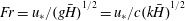
Figure 1. Sketch of the simulation set-up. The hollow arrow on the surface indicates the direction of wave propagation (with phase speed
 $c$
) and surface shear stress.
$c$
) and surface shear stress.
2 Problem set-up and numerical methods
In this section, we first introduce the problem set-up and governing equations in §§ 2.1 and 2.2. Then, the numerical method and the computational parameters are described in §§ 2.3 and 2.4, respectively. Finally, in § 2.5, we introduce a triple decomposition method that employs the theory of generalized Lagrangian mean (GLM) (Andrews & Mcintyre Reference Andrews and Mcintyre1978) to decompose the flow motions into the current, wave and turbulence for the subsequent analyses.
2.1 Problem set-up
For the mechanistic study of the wave–turbulence interaction processes, we consider a statistically steady turbulent flow driven by a monochromatic progressive wave, with a constant surface shear stress representing the wind shear applied on the surface. The simulations are performed in a horizontally periodic box bounded by a surface wave, as shown in figure 1. The wave propagation direction and the surface stress direction are aligned in the
 $x$
-direction. The shear stress is tangential to the wave surface in the
$x$
-direction. The shear stress is tangential to the wave surface in the
 $x$
–
$x$
–
 $z$
plane. A dynamic pressure forcing is imposed on the surface to keep the waves from decaying or distortion (Guo & Shen Reference Guo and Shen2009). With the constant wave and shear stress forcing, the Langmuir turbulence develops and reaches a statistically steady state, based on which we perform the analyses on the vorticity dynamics. We also note that the present study of Langmuir turbulence is different from the previous study of isotropic turbulence below a surface wave by Guo & Shen (Reference Guo and Shen2013, Reference Guo and Shen2014). In Langmuir turbulence, the turbulence is generated due to the wind shear applied at the wave surface and is modulated by the wave (Craik Reference Craik1977; Leibovich Reference Leibovich1977a
; Leibovich & Paolucci Reference Leibovich and Paolucci1980, Reference Leibovich and Paolucci1981). By contrast, in Guo & Shen (Reference Guo and Shen2013, Reference Guo and Shen2014), no wind shear stress is applied at the surface and isotropic turbulence is generated by a random force in the bulk flow. Therefore, these are two different problems.
$z$
plane. A dynamic pressure forcing is imposed on the surface to keep the waves from decaying or distortion (Guo & Shen Reference Guo and Shen2009). With the constant wave and shear stress forcing, the Langmuir turbulence develops and reaches a statistically steady state, based on which we perform the analyses on the vorticity dynamics. We also note that the present study of Langmuir turbulence is different from the previous study of isotropic turbulence below a surface wave by Guo & Shen (Reference Guo and Shen2013, Reference Guo and Shen2014). In Langmuir turbulence, the turbulence is generated due to the wind shear applied at the wave surface and is modulated by the wave (Craik Reference Craik1977; Leibovich Reference Leibovich1977a
; Leibovich & Paolucci Reference Leibovich and Paolucci1980, Reference Leibovich and Paolucci1981). By contrast, in Guo & Shen (Reference Guo and Shen2013, Reference Guo and Shen2014), no wind shear stress is applied at the surface and isotropic turbulence is generated by a random force in the bulk flow. Therefore, these are two different problems.
Because the present study focuses on the fundamental mechanism of the wave effect on the turbulence, we intentionally maintain a stationary surface wave to isolate the dynamical processes in the turbulence. We shall note that the current and turbulence underneath can also affect the wave field, including changing the dispersion relation (Kirby & Chen Reference Kirby and Chen1989; Swan, Cummins & James Reference Swan, Cummins and James2001) and inducing wave scattering and damping (Vivanco & Melo Reference Vivanco and Melo2004; Ardhuin & Jenkins Reference Ardhuin and Jenkins2006; Gutiérrez & Aumaître Reference Gutiérrez and Aumaître2016). Although the wave-phase-resolved simulation can be used to study the turbulence effect on the surface waves and the effect of temporal variation of the wave on the turbulence (Phillips Reference Phillips2002), they are beyond the scope of this research. In addition, as discussed in the following sections, the current and turbulence resulting from the set-up are weak compared with the wave orbital motions, and the wave field evolves slowly compared with the wave period (Thorpe Reference Thorpe2004). Therefore, it is reasonable to maintain a steady wave such that the wave effect on the turbulence can be quantified accurately.
2.2 Governing equations and boundary conditions
In this study, the turbulent flow is modelled by LES. For a fluid with constant density
 $\unicode[STIX]{x1D70C}$
and kinematic viscosity
$\unicode[STIX]{x1D70C}$
and kinematic viscosity
 $\unicode[STIX]{x1D708}$
, the grid-resolved flow motions in an Earth-fixed Eulerian frame are described by the filtered incompressible Navier–Stokes equations and continuity equation,
$\unicode[STIX]{x1D708}$
, the grid-resolved flow motions in an Earth-fixed Eulerian frame are described by the filtered incompressible Navier–Stokes equations and continuity equation,
 $$\begin{eqnarray}\displaystyle & \displaystyle \frac{\unicode[STIX]{x2202}u_{i}}{\unicode[STIX]{x2202}t}+\frac{\unicode[STIX]{x2202}(u_{i}u_{j})}{\unicode[STIX]{x2202}x_{j}}=-\frac{1}{\unicode[STIX]{x1D70C}}\frac{\unicode[STIX]{x2202}p}{\unicode[STIX]{x2202}x_{i}}+\unicode[STIX]{x1D708}\frac{\unicode[STIX]{x2202}^{2}u_{i}}{\unicode[STIX]{x2202}x_{j}x_{j}}-\frac{\unicode[STIX]{x2202}\unicode[STIX]{x1D70F}_{ij}^{d}}{\unicode[STIX]{x2202}x_{j}}, & \displaystyle\end{eqnarray}$$
 $$\begin{eqnarray}\displaystyle & \displaystyle \frac{\unicode[STIX]{x2202}u_{j}}{\unicode[STIX]{x2202}x_{j}}=0. & \displaystyle\end{eqnarray}$$
In the above equations,
 $x_{i}$
(
$x_{i}$
(
 $i=1,2,3$
) denote the Cartesian coordinates
$i=1,2,3$
) denote the Cartesian coordinates
 $(x,y,z)$
, respectively;
$(x,y,z)$
, respectively;
 $u_{i}$
denote the components of the filtered Eulerian velocity
$u_{i}$
denote the components of the filtered Eulerian velocity
 $(u,v,w)$
;
$(u,v,w)$
;
 $\unicode[STIX]{x1D70F}_{ij}^{d}=\unicode[STIX]{x1D70F}_{ij}-\unicode[STIX]{x1D70F}_{ii}/3$
(
$\unicode[STIX]{x1D70F}_{ij}^{d}=\unicode[STIX]{x1D70F}_{ij}-\unicode[STIX]{x1D70F}_{ii}/3$
(
 $i,j=1,2,3$
) is the trace-free part of the subgrid-scale (SGS) stress
$i,j=1,2,3$
) is the trace-free part of the subgrid-scale (SGS) stress
 $\unicode[STIX]{x1D70F}_{ij}$
; and
$\unicode[STIX]{x1D70F}_{ij}$
; and
 $p$
is the modified dynamic pressure, which includes the isotropic part of the SGS stress
$p$
is the modified dynamic pressure, which includes the isotropic part of the SGS stress
 $\unicode[STIX]{x1D70F}_{ii}/3$
.
$\unicode[STIX]{x1D70F}_{ii}/3$
.
At the free surface
 $z=\unicode[STIX]{x1D702}(x,y)$
, where
$z=\unicode[STIX]{x1D702}(x,y)$
, where
 $\unicode[STIX]{x1D702}$
is the surface elevation, we impose a constant tangential shear stress
$\unicode[STIX]{x1D702}$
is the surface elevation, we impose a constant tangential shear stress
 $\unicode[STIX]{x1D70F}_{0}$
in the
$\unicode[STIX]{x1D70F}_{0}$
in the
 $x$
–
$x$
–
 $z$
plane and a dynamic pressure
$z$
plane and a dynamic pressure
 $p_{a}$
. The value of
$p_{a}$
. The value of
 $p_{a}$
is determined based on the wave surface elevation and the surface velocity to maintain a monochromatic progressive wave (Guo & Shen Reference Guo and Shen2009). The work done by
$p_{a}$
is determined based on the wave surface elevation and the surface velocity to maintain a monochromatic progressive wave (Guo & Shen Reference Guo and Shen2009). The work done by
 $p_{a}$
compensates the wave energy loss such that the wave amplitude is sustained. The detailed form of
$p_{a}$
compensates the wave energy loss such that the wave amplitude is sustained. The detailed form of
 $p_{a}$
is given in appendix A. The stress balance at the interface is given by the dynamic boundary conditions (DBCs),
$p_{a}$
is given in appendix A. The stress balance at the interface is given by the dynamic boundary conditions (DBCs),
 $$\begin{eqnarray}\displaystyle & \displaystyle \boldsymbol{n}\boldsymbol{\cdot }\unicode[STIX]{x1D748}\boldsymbol{\cdot }\boldsymbol{n}^{\text{T}}=-p_{a}, & \displaystyle\end{eqnarray}$$
 $$\begin{eqnarray}\displaystyle & \displaystyle \boldsymbol{t}^{1}\boldsymbol{\cdot }\unicode[STIX]{x1D748}\boldsymbol{\cdot }\boldsymbol{n}^{\text{T}}=\unicode[STIX]{x1D70F}_{0}, & \displaystyle\end{eqnarray}$$
 $$\begin{eqnarray}\displaystyle & \displaystyle \boldsymbol{t}^{2}\boldsymbol{\cdot }\unicode[STIX]{x1D748}\boldsymbol{\cdot }\boldsymbol{n}^{\text{T}}=0. & \displaystyle\end{eqnarray}$$
 $p_{a}$
and shear stress
$p_{a}$
and shear stress
 $\unicode[STIX]{x1D70F}_{0}$
to the total stress tensor
$\unicode[STIX]{x1D70F}_{0}$
to the total stress tensor
 $\unicode[STIX]{x1D748}=-(p-\unicode[STIX]{x1D70C}gz)\unicode[STIX]{x1D644}+2\unicode[STIX]{x1D70C}\unicode[STIX]{x1D708}\unicode[STIX]{x1D64E}$
, where
$\unicode[STIX]{x1D748}=-(p-\unicode[STIX]{x1D70C}gz)\unicode[STIX]{x1D644}+2\unicode[STIX]{x1D70C}\unicode[STIX]{x1D708}\unicode[STIX]{x1D64E}$
, where
 $\unicode[STIX]{x1D644}$
is the identity tensor,
$\unicode[STIX]{x1D644}$
is the identity tensor,
 $g$
is the gravitational acceleration and
$g$
is the gravitational acceleration and
 $\unicode[STIX]{x1D64E}=(\unicode[STIX]{x1D735}\boldsymbol{u}+\unicode[STIX]{x1D735}\boldsymbol{u}^{\mathbf{T}})/2$
is the resolved strain rate tensor. Also in the above equations,
$\unicode[STIX]{x1D64E}=(\unicode[STIX]{x1D735}\boldsymbol{u}+\unicode[STIX]{x1D735}\boldsymbol{u}^{\mathbf{T}})/2$
is the resolved strain rate tensor. Also in the above equations,
 $\boldsymbol{n}$
is the surface normal vector;
$\boldsymbol{n}$
is the surface normal vector;
 $\boldsymbol{t}^{1}$
and
$\boldsymbol{t}^{1}$
and
 $\boldsymbol{t}^{2}$
are the surface tangential vectors in the
$\boldsymbol{t}^{2}$
are the surface tangential vectors in the
 $x$
–
$x$
–
 $z$
and
$z$
and
 $y$
–
$y$
–
 $z$
planes, respectively. These vectors are calculated by
$z$
planes, respectively. These vectors are calculated by  $$\begin{eqnarray}\boldsymbol{n}=\frac{(-\unicode[STIX]{x1D702}_{x},-\unicode[STIX]{x1D702}_{y},1)}{\sqrt{\unicode[STIX]{x1D702}_{x}^{2}+\unicode[STIX]{x1D702}_{y}^{2}+1}},\quad \boldsymbol{t}^{1}=\frac{(1,0,\unicode[STIX]{x1D702}_{x})}{\sqrt{1+\unicode[STIX]{x1D702}_{x}^{2}}},\quad \boldsymbol{t}^{2}=\frac{(0,1,\unicode[STIX]{x1D702}_{y})}{\sqrt{1+\unicode[STIX]{x1D702}_{y}^{2}}},\end{eqnarray}$$
where
 $\unicode[STIX]{x1D702}_{x}$
and
$\unicode[STIX]{x1D702}_{x}$
and
 $\unicode[STIX]{x1D702}_{y}$
denote
$\unicode[STIX]{x1D702}_{y}$
denote
 $\unicode[STIX]{x2202}\unicode[STIX]{x1D702}/\unicode[STIX]{x2202}x$
and
$\unicode[STIX]{x2202}\unicode[STIX]{x1D702}/\unicode[STIX]{x2202}x$
and
 $\unicode[STIX]{x2202}\unicode[STIX]{x1D702}/\unicode[STIX]{x2202}y$
, respectively.
$\unicode[STIX]{x2202}\unicode[STIX]{x1D702}/\unicode[STIX]{x2202}y$
, respectively.
The evolution of
 $\unicode[STIX]{x1D702}$
is governed by the kinematic boundary condition (KBC),
$\unicode[STIX]{x1D702}$
is governed by the kinematic boundary condition (KBC),
 $$\begin{eqnarray}\frac{\unicode[STIX]{x2202}\unicode[STIX]{x1D702}}{\unicode[STIX]{x2202}t}=w-u\unicode[STIX]{x1D702}_{x}-v\unicode[STIX]{x1D702}_{y},\quad \text{at }z=\unicode[STIX]{x1D702}.\end{eqnarray}$$
We note here that the SGS effect on the free-surface boundary conditions is still an open problem but is usually considered to be negligibly small (Hodges & Street Reference Hodges and Street1999; Dimas & Fialkowski Reference Dimas and Fialkowski2000). Meanwhile, the SGS effect on the boundary is minimized in the present study with a sufficient grid resolution to achieve wall-resolved LES (§ 2.4).
The bottom is free slip, where the velocity boundary condition is given by
 $$\begin{eqnarray}\frac{\unicode[STIX]{x2202}u}{\unicode[STIX]{x2202}z}=\frac{\unicode[STIX]{x2202}v}{\unicode[STIX]{x2202}z}=0,\quad w=0,\quad \text{at }z=-\bar{H}.\end{eqnarray}$$
Because the shear is often weak at the base of the ocean surface boundary layer (Belcher et al.
Reference Belcher, Grant, Hanley, Fox-Kemper, Van Roekel, Sullivan, Large, Brown, Hines and Calvert2012), the free-slip boundary condition is imposed to minimize the impact of the bottom of the domain as long as
 $\bar{H}$
is sufficiently large (Shen et al.
Reference Shen, Zhang, Yue and Triantafyllou1999). Under realistic conditions, body forces such as the Coriolis force balance the momentum. In this study, to focus on the mechanisms of the wave–turbulence interaction, we use a uniform adverse pressure gradient
$\bar{H}$
is sufficiently large (Shen et al.
Reference Shen, Zhang, Yue and Triantafyllou1999). Under realistic conditions, body forces such as the Coriolis force balance the momentum. In this study, to focus on the mechanisms of the wave–turbulence interaction, we use a uniform adverse pressure gradient
 $\unicode[STIX]{x2202}p/\unicode[STIX]{x2202}x=\unicode[STIX]{x1D70F}_{0}/\bar{H}$
to balance the shear stress at the upper surface so that the total momentum in the flow does not increase with time, which facilitates the analyses of statistics. The imposed pressure gradient is small compared to other effects (especially the wave forcing) in the system, therefore ought not to qualitatively change the fundamental mechanisms of the wave–turbulence interaction that we are interested in. More details of the magnitude of the forcing are discussed in § 2.4.
$\unicode[STIX]{x2202}p/\unicode[STIX]{x2202}x=\unicode[STIX]{x1D70F}_{0}/\bar{H}$
to balance the shear stress at the upper surface so that the total momentum in the flow does not increase with time, which facilitates the analyses of statistics. The imposed pressure gradient is small compared to other effects (especially the wave forcing) in the system, therefore ought not to qualitatively change the fundamental mechanisms of the wave–turbulence interaction that we are interested in. More details of the magnitude of the forcing are discussed in § 2.4.
The SGS stress
 $\unicode[STIX]{x1D70F}_{ij}^{d}$
in (2.1) is computed using a Lagrangian dynamic scale-dependent model (Bou-Zeid, Meneveau & Parlange Reference Bou-Zeid, Meneveau and Parlange2005)
$\unicode[STIX]{x1D70F}_{ij}^{d}$
in (2.1) is computed using a Lagrangian dynamic scale-dependent model (Bou-Zeid, Meneveau & Parlange Reference Bou-Zeid, Meneveau and Parlange2005)
 $$\begin{eqnarray}\unicode[STIX]{x1D70F}_{ij}^{d}=-2C_{\unicode[STIX]{x1D6E5}}|\unicode[STIX]{x1D61A}_{ij}|\unicode[STIX]{x1D61A}_{ij},\end{eqnarray}$$
where
 $|\unicode[STIX]{x1D61A}_{ij}|=\sqrt{2\unicode[STIX]{x1D61A}_{ij}\unicode[STIX]{x1D61A}_{ij}}$
is the magnitude of the tensor
$|\unicode[STIX]{x1D61A}_{ij}|=\sqrt{2\unicode[STIX]{x1D61A}_{ij}\unicode[STIX]{x1D61A}_{ij}}$
is the magnitude of the tensor
 $\unicode[STIX]{x1D61A}_{ij}$
and
$\unicode[STIX]{x1D61A}_{ij}$
and
 $C_{\unicode[STIX]{x1D6E5}}$
is the Smagorinsky coefficient. The
$C_{\unicode[STIX]{x1D6E5}}$
is the Smagorinsky coefficient. The
 $C_{\unicode[STIX]{x1D6E5}}$
is dynamically determined based on the weighted average of the flow information along pathlines. The dynamic model removes the necessity to determine
$C_{\unicode[STIX]{x1D6E5}}$
is dynamically determined based on the weighted average of the flow information along pathlines. The dynamic model removes the necessity to determine
 $C_{\unicode[STIX]{x1D6E5}}$
on an ad hoc basis (Germano et al.
Reference Germano, Piomelli, Moin and Cabot1991), and the Lagrangian average formulation improves the model’s capability to address the inhomogeneity in flows with complex geometries (Meneveau, Lund & Cabot Reference Meneveau, Lund and Cabot1996; Stoll & Porté-Agel Reference Stoll and Porté-Agel2006; Yang, Meneveau & Shen Reference Yang, Meneveau and Shen2014b
,Reference Yang, Meneveau and Shen
c
), such as the waves in the present study. This model also takes the scale dependency of
$C_{\unicode[STIX]{x1D6E5}}$
on an ad hoc basis (Germano et al.
Reference Germano, Piomelli, Moin and Cabot1991), and the Lagrangian average formulation improves the model’s capability to address the inhomogeneity in flows with complex geometries (Meneveau, Lund & Cabot Reference Meneveau, Lund and Cabot1996; Stoll & Porté-Agel Reference Stoll and Porté-Agel2006; Yang, Meneveau & Shen Reference Yang, Meneveau and Shen2014b
,Reference Yang, Meneveau and Shen
c
), such as the waves in the present study. This model also takes the scale dependency of
 $C_{\unicode[STIX]{x1D6E5}}$
into consideration. Traditional dynamic model applies a test filter with scale
$C_{\unicode[STIX]{x1D6E5}}$
into consideration. Traditional dynamic model applies a test filter with scale
 $\widetilde{\unicode[STIX]{x1D6E5}}$
(typically
$\widetilde{\unicode[STIX]{x1D6E5}}$
(typically
 $\widetilde{\unicode[STIX]{x1D6E5}}=2\unicode[STIX]{x1D6E5}$
) to the resolved velocity and calculates
$\widetilde{\unicode[STIX]{x1D6E5}}=2\unicode[STIX]{x1D6E5}$
) to the resolved velocity and calculates
 $C_{\unicode[STIX]{x1D6E5}}$
using the flow information at both grid filter scale and test filter scale. The calculation utilizes the assumption that
$C_{\unicode[STIX]{x1D6E5}}$
using the flow information at both grid filter scale and test filter scale. The calculation utilizes the assumption that
 $C_{\unicode[STIX]{x1D6E5}}$
does not depend on the filter scale, i.e.
$C_{\unicode[STIX]{x1D6E5}}$
does not depend on the filter scale, i.e.
 $C_{\unicode[STIX]{x1D6E5}}=C_{\widetilde{\unicode[STIX]{x1D6E5}}}$
. However, it is found that the scale-invariance assumption does not always hold, especially near the boundary (Porté-Agel, Meneveau & Parlange Reference Porté-Agel, Meneveau and Parlange2000). The scale-dependent model introduces another test filter with width
$C_{\unicode[STIX]{x1D6E5}}=C_{\widetilde{\unicode[STIX]{x1D6E5}}}$
. However, it is found that the scale-invariance assumption does not always hold, especially near the boundary (Porté-Agel, Meneveau & Parlange Reference Porté-Agel, Meneveau and Parlange2000). The scale-dependent model introduces another test filter with width
 $\hat{\unicode[STIX]{x1D6E5}}$
(e.g.
$\hat{\unicode[STIX]{x1D6E5}}$
(e.g.
 $\hat{\unicode[STIX]{x1D6E5}}=2\widetilde{\unicode[STIX]{x1D6E5}}=4\unicode[STIX]{x1D6E5}$
) and is thus able to determine how the Smagorinsky coefficient varies with the filter width using three levels of the filtered flow fields. This tuning-free scale-dependent model has been shown to yield good predictions of near-surface flow features (Porté-Agel et al.
Reference Porté-Agel, Meneveau and Parlange2000).
$\hat{\unicode[STIX]{x1D6E5}}=2\widetilde{\unicode[STIX]{x1D6E5}}=4\unicode[STIX]{x1D6E5}$
) and is thus able to determine how the Smagorinsky coefficient varies with the filter width using three levels of the filtered flow fields. This tuning-free scale-dependent model has been shown to yield good predictions of near-surface flow features (Porté-Agel et al.
Reference Porté-Agel, Meneveau and Parlange2000).
2.3 Numerical methods
The governing equations (2.1) and (2.2) are transformed to and solved on a surface-boundary-fitted curvilinear coordinate system
 $(\unicode[STIX]{x1D709}^{i},\unicode[STIX]{x1D70F})$
. The numerical approach (Yang & Shen Reference Yang and Shen2011; Xuan & Shen Reference Xuan and Shen2019) has been proven to be accurate and effective in resolving the flow details in the wave boundary layer, e.g. the distortion effects of waves on turbulence (Guo & Shen Reference Guo and Shen2013, Reference Guo and Shen2014) and wind–wave interactions (Yang, Meneveau & Shen Reference Yang, Meneveau and Shen2013; Yang et al.
Reference Yang, Meneveau and Shen2014c
).
$(\unicode[STIX]{x1D709}^{i},\unicode[STIX]{x1D70F})$
. The numerical approach (Yang & Shen Reference Yang and Shen2011; Xuan & Shen Reference Xuan and Shen2019) has been proven to be accurate and effective in resolving the flow details in the wave boundary layer, e.g. the distortion effects of waves on turbulence (Guo & Shen Reference Guo and Shen2013, Reference Guo and Shen2014) and wind–wave interactions (Yang, Meneveau & Shen Reference Yang, Meneveau and Shen2013; Yang et al.
Reference Yang, Meneveau and Shen2014c
).
The transformation between the Cartesian and curvilinear coordinates is defined as
 $$\begin{eqnarray}\unicode[STIX]{x1D709}^{1}=x_{1},\quad \unicode[STIX]{x1D709}^{2}=x_{2},\quad \unicode[STIX]{x1D709}^{3}=\frac{z+\bar{H}}{\unicode[STIX]{x1D702}+\bar{H}},\quad \unicode[STIX]{x1D70F}=t.\end{eqnarray}$$
Hereafter,
 $(\unicode[STIX]{x1D709}^{1},\unicode[STIX]{x1D709}^{2},\unicode[STIX]{x1D709}^{3})$
are also denoted as
$(\unicode[STIX]{x1D709}^{1},\unicode[STIX]{x1D709}^{2},\unicode[STIX]{x1D709}^{3})$
are also denoted as
 $(\unicode[STIX]{x1D709},\unicode[STIX]{x1D713},\unicode[STIX]{x1D701})$
. In the transformation (2.8), the varying depth in the physical space is normalized to a unit dimension in the curvilinear coordinates (
$(\unicode[STIX]{x1D709},\unicode[STIX]{x1D713},\unicode[STIX]{x1D701})$
. In the transformation (2.8), the varying depth in the physical space is normalized to a unit dimension in the curvilinear coordinates (
 $0\leqslant \unicode[STIX]{x1D701}\leqslant 1$
). As an example, the transformation of a vertical
$0\leqslant \unicode[STIX]{x1D701}\leqslant 1$
). As an example, the transformation of a vertical
 $x$
–
$x$
–
 $z$
plane is illustrated in figure 2, where the curvilinear coordinate curves for
$z$
plane is illustrated in figure 2, where the curvilinear coordinate curves for
 $\unicode[STIX]{x1D709}$
and
$\unicode[STIX]{x1D709}$
and
 $\unicode[STIX]{x1D701}$
are plotted schematically.
$\unicode[STIX]{x1D701}$
are plotted schematically.

Figure 2. Curvilinear coordinates used in the simulations. Only one
 $x$
–
$x$
–
 $z$
(
$z$
(
 $\unicode[STIX]{x1D709}$
–
$\unicode[STIX]{x1D709}$
–
 $\unicode[STIX]{x1D701}$
) plane is shown.
$\unicode[STIX]{x1D701}$
) plane is shown.
Applying (2.8) to (2.1) and (2.2), we obtain the governing equations under the curvilinear coordinates as
 $$\begin{eqnarray}\displaystyle & & \displaystyle \frac{\unicode[STIX]{x2202}(J^{-1}u_{i})}{\unicode[STIX]{x2202}\unicode[STIX]{x1D70F}}-\frac{\unicode[STIX]{x2202}(J^{-1}U_{g}^{j}u_{i})}{\unicode[STIX]{x2202}\unicode[STIX]{x1D709}^{j}}+\frac{\unicode[STIX]{x2202}(J^{-1}U_{j}u_{i})}{\unicode[STIX]{x2202}\unicode[STIX]{x1D709}^{j}}\nonumber\\ \displaystyle & & \displaystyle \quad =-\frac{\unicode[STIX]{x2202}}{\unicode[STIX]{x2202}\unicode[STIX]{x1D709}^{j}}\left(J^{-1}\frac{\unicode[STIX]{x2202}\unicode[STIX]{x1D709}^{j}}{\unicode[STIX]{x2202}x_{i}}p\right)+\frac{1}{Re}\frac{\unicode[STIX]{x2202}}{\unicode[STIX]{x2202}\unicode[STIX]{x1D709}^{j}}\left(J^{-1}g^{ij}\frac{\unicode[STIX]{x2202}u_{i}}{\unicode[STIX]{x2202}\unicode[STIX]{x1D709}^{j}}\right)-\frac{\unicode[STIX]{x2202}}{\unicode[STIX]{x2202}\unicode[STIX]{x1D709}^{k}}\left(J^{-1}\frac{\unicode[STIX]{x2202}\unicode[STIX]{x1D709}^{k}}{\unicode[STIX]{x2202}x_{j}}\unicode[STIX]{x1D70F}_{ij}^{d}\right),\end{eqnarray}$$
 $$\begin{eqnarray}\frac{\unicode[STIX]{x2202}U^{j}}{\unicode[STIX]{x2202}\unicode[STIX]{x1D709}^{j}}=0.\end{eqnarray}$$
Here,
 $U^{i}=u_{k}(\unicode[STIX]{x2202}\unicode[STIX]{x1D709}^{i}/\unicode[STIX]{x2202}x_{k})$
is the contravariant velocity;
$U^{i}=u_{k}(\unicode[STIX]{x2202}\unicode[STIX]{x1D709}^{i}/\unicode[STIX]{x2202}x_{k})$
is the contravariant velocity;
 $U_{g}^{i}=\unicode[STIX]{x1D6FF}_{k3}\unicode[STIX]{x1D702}_{t}\unicode[STIX]{x1D709}^{3}(\unicode[STIX]{x2202}\unicode[STIX]{x1D709}^{i}/\unicode[STIX]{x2202}x_{k})$
is the contravariant grid velocity;
$U_{g}^{i}=\unicode[STIX]{x1D6FF}_{k3}\unicode[STIX]{x1D702}_{t}\unicode[STIX]{x1D709}^{3}(\unicode[STIX]{x2202}\unicode[STIX]{x1D709}^{i}/\unicode[STIX]{x2202}x_{k})$
is the contravariant grid velocity;
 $J=\det (\unicode[STIX]{x2202}\unicode[STIX]{x1D709}^{i}/\unicode[STIX]{x2202}x_{j})$
is the Jacobian determinant of the transformation;
$J=\det (\unicode[STIX]{x2202}\unicode[STIX]{x1D709}^{i}/\unicode[STIX]{x2202}x_{j})$
is the Jacobian determinant of the transformation;
 $g^{ij}=(\unicode[STIX]{x2202}\unicode[STIX]{x1D709}^{i}/\unicode[STIX]{x2202}x_{k})(\unicode[STIX]{x2202}\unicode[STIX]{x1D709}^{j}/\unicode[STIX]{x2202}x_{k})$
is the metric tensor of the transformation. We remark that the above equations are written and discretized in a strong conservative form under the curvilinear coordinates. We find that this practice greatly improves the conservation of mass and momentum in the simulations. The velocity and time scales in Langmuir turbulence span over a wide range. The turbulent motions generally have much smaller velocity than the wave-induced orbital velocity, and have a much longer characteristic time scale of evolution than the wave period. The disparate scales make the simulation of turbulence prone to the contamination by numerical errors. We find that the strong conservative scheme greatly reduces the numerical errors in mass and momentum conservations (Xuan & Shen Reference Xuan and Shen2019).
$g^{ij}=(\unicode[STIX]{x2202}\unicode[STIX]{x1D709}^{i}/\unicode[STIX]{x2202}x_{k})(\unicode[STIX]{x2202}\unicode[STIX]{x1D709}^{j}/\unicode[STIX]{x2202}x_{k})$
is the metric tensor of the transformation. We remark that the above equations are written and discretized in a strong conservative form under the curvilinear coordinates. We find that this practice greatly improves the conservation of mass and momentum in the simulations. The velocity and time scales in Langmuir turbulence span over a wide range. The turbulent motions generally have much smaller velocity than the wave-induced orbital velocity, and have a much longer characteristic time scale of evolution than the wave period. The disparate scales make the simulation of turbulence prone to the contamination by numerical errors. We find that the strong conservative scheme greatly reduces the numerical errors in mass and momentum conservations (Xuan & Shen Reference Xuan and Shen2019).
The horizontal directions
 $\unicode[STIX]{x1D709}$
and
$\unicode[STIX]{x1D709}$
and
 $\unicode[STIX]{x1D713}$
are discretized by uniformly distributed Fourier collocation points. The spatial derivatives with respect to
$\unicode[STIX]{x1D713}$
are discretized by uniformly distributed Fourier collocation points. The spatial derivatives with respect to
 $\unicode[STIX]{x1D709}$
and
$\unicode[STIX]{x1D709}$
and
 $\unicode[STIX]{x1D713}$
are obtained in the spectral space. The discretization in the
$\unicode[STIX]{x1D713}$
are obtained in the spectral space. The discretization in the
 $\unicode[STIX]{x1D701}$
-direction employs a second-order finite-difference scheme, which allows more flexibility in the grid distribution to have fine resolution near the water surface. A staggered arrangement of the locations of the dependent variables is used in the
$\unicode[STIX]{x1D701}$
-direction employs a second-order finite-difference scheme, which allows more flexibility in the grid distribution to have fine resolution near the water surface. A staggered arrangement of the locations of the dependent variables is used in the
 $\unicode[STIX]{x1D701}$
-direction to avoid the odd–even decoupling. The velocity components
$\unicode[STIX]{x1D701}$
-direction to avoid the odd–even decoupling. The velocity components
 $(u,v)$
,
$(u,v)$
,
 $(U,V)$
and the pressure
$(U,V)$
and the pressure
 $p$
are located at the cell centre, while
$p$
are located at the cell centre, while
 $w$
and
$w$
and
 $W$
are located half a grid spacing off at the cell face.
$W$
are located half a grid spacing off at the cell face.
The solution of the Navier–Stokes equations (2.10) is coupled with the evolution of the free surface. The surface elevation
 $\unicode[STIX]{x1D702}(x,y,t)$
is obtained from the integration of (2.5) using a two-stage Runge–Kutta scheme,
$\unicode[STIX]{x1D702}(x,y,t)$
is obtained from the integration of (2.5) using a two-stage Runge–Kutta scheme,
 $$\begin{eqnarray}\displaystyle & \displaystyle \text{Stage I:}\quad \hat{\unicode[STIX]{x1D702}}=\unicode[STIX]{x1D702}|_{t}+\unicode[STIX]{x0394}t(w-u\unicode[STIX]{x1D702}_{x}-v\unicode[STIX]{x1D702}_{y})|_{t}, & \displaystyle\end{eqnarray}$$
 $$\begin{eqnarray}\displaystyle & \displaystyle \text{Stage II:}\quad \unicode[STIX]{x1D702}|_{t+\unicode[STIX]{x0394}t}=\hat{\unicode[STIX]{x1D702}}-\frac{\unicode[STIX]{x0394}t}{2}(w-u\unicode[STIX]{x1D702}_{x}-v\unicode[STIX]{x1D702}_{y})|_{t}+\frac{\unicode[STIX]{x0394}t}{2}({\hat{w}}-\hat{u} \hat{\unicode[STIX]{x1D702}}_{x}-\hat{v}\hat{\unicode[STIX]{x1D702}}_{y}), & \displaystyle\end{eqnarray}$$
 $\hat{(\cdot )}$
denotes the intermediate prediction at
$\hat{(\cdot )}$
denotes the intermediate prediction at
 $t+\unicode[STIX]{x0394}t$
, and
$t+\unicode[STIX]{x0394}t$
, and
 $(\cdot )|_{t}$
denotes the terms evaluated at time
$(\cdot )|_{t}$
denotes the terms evaluated at time
 $t$
. In each stage after obtaining
$t$
. In each stage after obtaining
 $\unicode[STIX]{x1D702}$
, the Navier–Stokes equations (2.9) are integrated using a fractional-step method (Kim & Moin Reference Kim and Moin1985) to update the velocity in the new domain bounded by the water surface. The procedures to advance the system from
$\unicode[STIX]{x1D702}$
, the Navier–Stokes equations (2.9) are integrated using a fractional-step method (Kim & Moin Reference Kim and Moin1985) to update the velocity in the new domain bounded by the water surface. The procedures to advance the system from
 $t$
to
$t$
to
 $t+\unicode[STIX]{x0394}t$
are as follows,
$t+\unicode[STIX]{x0394}t$
are as follows,(i) Obtain
 $\hat{\unicode[STIX]{x1D702}}$
using (2.11a
).
$\hat{\unicode[STIX]{x1D702}}$
using (2.11a
).(ii) Calculate
$\hat{\boldsymbol{u}}$
and
$\hat{p}$
in the domain with the elevation
$\hat{\unicode[STIX]{x1D702}}$
by integrating equations (2.9) from
$t$
to
$t+\unicode[STIX]{x0394}t$
subject to the constraint (2.10).(iii) Obtain the corrected surface elevation
$\unicode[STIX]{x1D702}|_{t+\unicode[STIX]{x0394}t}$
using (2.11b
).(iv) Calculate
$\boldsymbol{u}$
and
$p$
in the domain with the elevation
$\unicode[STIX]{x1D702}|_{t+\unicode[STIX]{x0394}t}$
by integrating (2.9) again from
$t$
to
$t+\unicode[STIX]{x0394}t$
as in the step (ii), but with the corrected elevation
$\unicode[STIX]{x1D702}|_{t+\unicode[STIX]{x0394}t}$
.


The velocity and pressure obtained from the above step (iv) are the solution of the flow field at
 $t+\unicode[STIX]{x0394}t$
. The above method has been tested extensively by Xuan & Shen (Reference Xuan and Shen2019).
$t+\unicode[STIX]{x0394}t$
. The above method has been tested extensively by Xuan & Shen (Reference Xuan and Shen2019).
2.4 Computational parameters
In the present study, we mainly focus on the effects of the wave on the turbulence, therefore simulations with different turbulent Langmuir numbers
 $La_{t}=\sqrt{u_{\ast }/U_{s}}$
and wave steepness
$La_{t}=\sqrt{u_{\ast }/U_{s}}$
and wave steepness
 $ak$
are considered (table 1). The turbulent Langmuir number (McWilliams et al.
Reference McWilliams, Sullivan and Moeng1997) associated with the friction velocity of wind-driven shear
$ak$
are considered (table 1). The turbulent Langmuir number (McWilliams et al.
Reference McWilliams, Sullivan and Moeng1997) associated with the friction velocity of wind-driven shear
 $u_{\ast }$
and the surface Stokes drift
$u_{\ast }$
and the surface Stokes drift
 $U_{s}$
is an important dimensionless parameter quantifying the relative strength of wind shear forcing versus wave forcing. A smaller
$U_{s}$
is an important dimensionless parameter quantifying the relative strength of wind shear forcing versus wave forcing. A smaller
 $La_{t}$
indicates stronger wave effects and stronger Langmuir turbulence. The friction velocity
$La_{t}$
indicates stronger wave effects and stronger Langmuir turbulence. The friction velocity
 $u_{\ast }$
is associated with the imposed shear stress
$u_{\ast }$
is associated with the imposed shear stress
 $\unicode[STIX]{x1D70F}_{0}$
by
$\unicode[STIX]{x1D70F}_{0}$
by
 $u_{\ast }=\sqrt{\unicode[STIX]{x1D70F}_{0}/\unicode[STIX]{x1D70C}}$
. The
$u_{\ast }=\sqrt{\unicode[STIX]{x1D70F}_{0}/\unicode[STIX]{x1D70C}}$
. The
 $La_{t}$
ranges from 0.35 to 0.9, corresponding to cases with strong to weak wave forcing. Strong Langmuir turbulence is expected when the wave forcing dominates over the shear stress forcing. The flow features change to those of the shear-driven turbulence as
$La_{t}$
ranges from 0.35 to 0.9, corresponding to cases with strong to weak wave forcing. Strong Langmuir turbulence is expected when the wave forcing dominates over the shear stress forcing. The flow features change to those of the shear-driven turbulence as
 $La_{t}$
increases (Li et al.
Reference Li, Garrett and Skyllingstad2005). The
$La_{t}$
increases (Li et al.
Reference Li, Garrett and Skyllingstad2005). The
 $La_{t}$
values considered above are consistent with the range of typical ocean conditions (Thorpe Reference Thorpe2004). The case S is a pure shear-driven turbulent flow with no prescribed waves for comparison with the Langmuir turbulence cases. For cases L1, L2 and L3, we set the wave steepness
$La_{t}$
values considered above are consistent with the range of typical ocean conditions (Thorpe Reference Thorpe2004). The case S is a pure shear-driven turbulent flow with no prescribed waves for comparison with the Langmuir turbulence cases. For cases L1, L2 and L3, we set the wave steepness
 $ak$
to
$ak$
to
 $0.084$
, where
$0.084$
, where
 $a$
and
$a$
and
 $k$
are the amplitude and the wavenumber of the surface wave, respectively. A case L1S with a steeper wave but the same
$k$
are the amplitude and the wavenumber of the surface wave, respectively. A case L1S with a steeper wave but the same
 $La_{t}$
as in case L1 is set up to study the effects of wave steepness. The dimensionless wavenumber
$La_{t}$
as in case L1 is set up to study the effects of wave steepness. The dimensionless wavenumber
 $k\bar{H}$
is set to
$k\bar{H}$
is set to
 $3.5$
, corresponding to a deep-water wave with wavelength
$3.5$
, corresponding to a deep-water wave with wavelength
 $\unicode[STIX]{x1D706}=4\unicode[STIX]{x03C0}\bar{H}/7$
. The remaining wave-related parameters in table 1 are derived from
$\unicode[STIX]{x1D706}=4\unicode[STIX]{x03C0}\bar{H}/7$
. The remaining wave-related parameters in table 1 are derived from
 $La_{t}$
,
$La_{t}$
,
 $ak$
and
$ak$
and
 $k\bar{H}$
using the estimation from the linear wave theory. The surface Stokes drift is related to the wave phase speed
$k\bar{H}$
using the estimation from the linear wave theory. The surface Stokes drift is related to the wave phase speed
 $c$
through
$c$
through
 $U_{s}=(ak)^{2}c$
according to the linear wave theory, and thus
$U_{s}=(ak)^{2}c$
according to the linear wave theory, and thus
 $c/u_{\ast }=(ak)^{-2}La_{t}^{-2}$
. The wave frequency
$c/u_{\ast }=(ak)^{-2}La_{t}^{-2}$
. The wave frequency
 $\unicode[STIX]{x1D714}=ck$
normalized by the shear strain rate
$\unicode[STIX]{x1D714}=ck$
normalized by the shear strain rate
 $u_{\ast }/\bar{H}$
is
$u_{\ast }/\bar{H}$
is
 $\unicode[STIX]{x1D714}/(u_{\ast }\bar{H}^{-1})=(c/u_{\ast })(k\bar{H})$
, which also represents the ratio of the wave frequency to the frequency of the eddy turnover motion in the turbulent flow. Also given in table 1 is the Froude number
$\unicode[STIX]{x1D714}/(u_{\ast }\bar{H}^{-1})=(c/u_{\ast })(k\bar{H})$
, which also represents the ratio of the wave frequency to the frequency of the eddy turnover motion in the turbulent flow. Also given in table 1 is the Froude number
 $Fr=u_{\ast }/(g\bar{H})^{1/2}=u_{\ast }/c(k\bar{H})^{1/2}$
. For reference, we provide an example of the typical dimensional parameters that correspond to case L1. The wavelength and the wavenumber for the surface wave are
$Fr=u_{\ast }/(g\bar{H})^{1/2}=u_{\ast }/c(k\bar{H})^{1/2}$
. For reference, we provide an example of the typical dimensional parameters that correspond to case L1. The wavelength and the wavenumber for the surface wave are
 $\unicode[STIX]{x1D706}=60~\text{m}$
and
$\unicode[STIX]{x1D706}=60~\text{m}$
and
 $k=2\unicode[STIX]{x03C0}/\unicode[STIX]{x1D706}=0.105~\text{m}^{-1}$
, respectively, which have been used in LES of Langmuir circulation (McWilliams et al.
Reference McWilliams, Sullivan and Moeng1997; Li et al.
Reference Li, Garrett and Skyllingstad2005). The corresponding surface Stokes drift is
$k=2\unicode[STIX]{x03C0}/\unicode[STIX]{x1D706}=0.105~\text{m}^{-1}$
, respectively, which have been used in LES of Langmuir circulation (McWilliams et al.
Reference McWilliams, Sullivan and Moeng1997; Li et al.
Reference Li, Garrett and Skyllingstad2005). The corresponding surface Stokes drift is
 $U_{s}=0.068~\text{m}~\text{s}^{-1}$
, and the friction velocity is
$U_{s}=0.068~\text{m}~\text{s}^{-1}$
, and the friction velocity is
 $u_{\ast }=8.3\times 10^{-3}~\text{m}~\text{s}^{-1}$
.
$u_{\ast }=8.3\times 10^{-3}~\text{m}~\text{s}^{-1}$
.
Table 1. Computational parameters of Langmuir turbulence in the present study.

With the parameters above, we can compare the relative magnitudes of the different quantities in the system. As shown in table 1, the velocity scale of the current and turbulent motions, being
 $O(u_{\ast })$
, is much smaller than the wave phase speed
$O(u_{\ast })$
, is much smaller than the wave phase speed
 $c$
. As a result, it is expected that the modification of the current on the wave propagation is small. The separation of the velocity scales also corresponds to disparate forcing scales. The straining rate due to the wave orbital velocity, associated with the direct forcing of the wave applied on the turbulence, is
$c$
. As a result, it is expected that the modification of the current on the wave propagation is small. The separation of the velocity scales also corresponds to disparate forcing scales. The straining rate due to the wave orbital velocity, associated with the direct forcing of the wave applied on the turbulence, is
 $O(ak\unicode[STIX]{x1D714})$
. This is significantly larger than the shearing of the current, which is
$O(ak\unicode[STIX]{x1D714})$
. This is significantly larger than the shearing of the current, which is
 $O(u_{\ast }/\bar{H})$
, as shown in the last column of table 1. Using the wave strain rate, the forcing of the wave straining on the turbulence is estimated to be
$O(u_{\ast }/\bar{H})$
, as shown in the last column of table 1. Using the wave strain rate, the forcing of the wave straining on the turbulence is estimated to be
 $O(\unicode[STIX]{x1D70C}ak\unicode[STIX]{x1D714}u_{\ast })$
, which is much larger than the applied pressure gradient
$O(\unicode[STIX]{x1D70C}ak\unicode[STIX]{x1D714}u_{\ast })$
, which is much larger than the applied pressure gradient
 $\unicode[STIX]{x1D70C}u_{\ast }^{2}/\bar{H}$
, also shown in the last column of table 1.
$\unicode[STIX]{x1D70C}u_{\ast }^{2}/\bar{H}$
, also shown in the last column of table 1.
For the
 $60~\text{m}$
wave in oceans with a
$60~\text{m}$
wave in oceans with a
 $8.3\times 10^{-3}~\text{m}~\text{s}^{-1}$
friction velocity discussed above,
$8.3\times 10^{-3}~\text{m}~\text{s}^{-1}$
friction velocity discussed above,
 $Re_{\unicode[STIX]{x1D70F}}=u_{\ast }\bar{H}/\unicode[STIX]{x1D708}$
is
$Re_{\unicode[STIX]{x1D70F}}=u_{\ast }\bar{H}/\unicode[STIX]{x1D708}$
is
 $O(10^{5})$
. To have the same Reynolds number, the LES would need wall-layer modelling. However, the accuracy of wall-layer modelling in wave-phase-resolved free-surface simulation is still unknown. Here, for the purposes of mechanistic study of wave–turbulence interactions and establishing an accurate dataset for future wall-layer modelling study, we choose to perform wall-resolved LES at a moderate Reynolds number
$O(10^{5})$
. To have the same Reynolds number, the LES would need wall-layer modelling. However, the accuracy of wall-layer modelling in wave-phase-resolved free-surface simulation is still unknown. Here, for the purposes of mechanistic study of wave–turbulence interactions and establishing an accurate dataset for future wall-layer modelling study, we choose to perform wall-resolved LES at a moderate Reynolds number
 $Re_{\unicode[STIX]{x1D70F}}=2000$
such that the near-surface dynamics of wave–turbulence interactions is captured accurately. We note that some previous CL equations based study of Langmuir turbulence also employed the wall-resolved LES approach with reduced Reynolds number to resolve the boundary layer for mechanistic study (see e.g. Tejada-Martínez et al. (Reference Tejada-Martínez, Grosch, Gargett, Polton, Smith and MacKinnon2009) and more discussions in Deng et al. (Reference Deng, Yang, Xuan and Shen2019) recently). In the future, after the wall-layer modelling is validated for wave-phase-resolved LES of free-surface turbulence, it would be desirable to perform wall-modelled wave-phase-resolved LES for Langmuir turbulence with realistic Reynolds number directly. All the simulations are performed in a domain with a size
$Re_{\unicode[STIX]{x1D70F}}=2000$
such that the near-surface dynamics of wave–turbulence interactions is captured accurately. We note that some previous CL equations based study of Langmuir turbulence also employed the wall-resolved LES approach with reduced Reynolds number to resolve the boundary layer for mechanistic study (see e.g. Tejada-Martínez et al. (Reference Tejada-Martínez, Grosch, Gargett, Polton, Smith and MacKinnon2009) and more discussions in Deng et al. (Reference Deng, Yang, Xuan and Shen2019) recently). In the future, after the wall-layer modelling is validated for wave-phase-resolved LES of free-surface turbulence, it would be desirable to perform wall-modelled wave-phase-resolved LES for Langmuir turbulence with realistic Reynolds number directly. All the simulations are performed in a domain with a size
 $L_{x}\times L_{y}\times \bar{H}=16\unicode[STIX]{x03C0}\bar{H}/7\times 16\unicode[STIX]{x03C0}\bar{H}/7\times \bar{H}$
. This domain allows four periods of the wave in the
$L_{x}\times L_{y}\times \bar{H}=16\unicode[STIX]{x03C0}\bar{H}/7\times 16\unicode[STIX]{x03C0}\bar{H}/7\times \bar{H}$
. This domain allows four periods of the wave in the
 $x$
-direction. The domain size is comparable with previous simulations based on the CL equations in terms of the ratio of the mixed layer depth to the horizontal lengths (McWilliams et al.
Reference McWilliams, Sullivan and Moeng1997; Li et al.
Reference Li, Garrett and Skyllingstad2005; Kukulka et al.
Reference Kukulka, Plueddemann, Trowbridge and Sullivan2009). The domain size is further confirmed to be sufficiently large according to the two-point auto-correlation (appendix B). The domain is discretized by a grid of
$x$
-direction. The domain size is comparable with previous simulations based on the CL equations in terms of the ratio of the mixed layer depth to the horizontal lengths (McWilliams et al.
Reference McWilliams, Sullivan and Moeng1997; Li et al.
Reference Li, Garrett and Skyllingstad2005; Kukulka et al.
Reference Kukulka, Plueddemann, Trowbridge and Sullivan2009). The domain size is further confirmed to be sufficiently large according to the two-point auto-correlation (appendix B). The domain is discretized by a grid of
 $288\times 512\times 217$
points. The horizontal discretization is uniform with the streamwise and spanwise grid resolutions being
$288\times 512\times 217$
points. The horizontal discretization is uniform with the streamwise and spanwise grid resolutions being
 $\unicode[STIX]{x0394}x^{+}=49.9$
and
$\unicode[STIX]{x0394}x^{+}=49.9$
and
 $\unicode[STIX]{x0394}y^{+}=28.0$
, respectively. The vertical grid is condensed near the free surface, where the minimum grid spacing is
$\unicode[STIX]{x0394}y^{+}=28.0$
, respectively. The vertical grid is condensed near the free surface, where the minimum grid spacing is
 $\unicode[STIX]{x0394}z^{+}|_{\mathit{min}}=0.49$
. Here, the superscript ‘
$\unicode[STIX]{x0394}z^{+}|_{\mathit{min}}=0.49$
. Here, the superscript ‘
 $+$
’ denotes the wall-unit length defined as
$+$
’ denotes the wall-unit length defined as
 $x_{i}^{+}=x_{i}u_{\ast }/\unicode[STIX]{x1D708}$
. The grid resolution satisfies the requirement of boundary-resolving approach, i.e.
$x_{i}^{+}=x_{i}u_{\ast }/\unicode[STIX]{x1D708}$
. The grid resolution satisfies the requirement of boundary-resolving approach, i.e.
 $\unicode[STIX]{x0394}x^{+}\simeq 50$
,
$\unicode[STIX]{x0394}x^{+}\simeq 50$
,
 $\unicode[STIX]{x0394}y^{+}\simeq 30$
and
$\unicode[STIX]{x0394}y^{+}\simeq 30$
and
 $\unicode[STIX]{x0394}z^{+}|_{\mathit{min}}<1$
, which is needed for resolving the small-scale longitudinal vortical structures in the viscous sublayer that typically have a streamwise length of a few hundred wall units and a spanwise spacing of approximately 100 wall units (Chapman Reference Chapman1979; Piomelli & Balaras Reference Piomelli and Balaras2002; Choi & Moin Reference Choi and Moin2012; Yang et al.
Reference Yang, Meneveau and Shen2013).
$\unicode[STIX]{x0394}z^{+}|_{\mathit{min}}<1$
, which is needed for resolving the small-scale longitudinal vortical structures in the viscous sublayer that typically have a streamwise length of a few hundred wall units and a spanwise spacing of approximately 100 wall units (Chapman Reference Chapman1979; Piomelli & Balaras Reference Piomelli and Balaras2002; Choi & Moin Reference Choi and Moin2012; Yang et al.
Reference Yang, Meneveau and Shen2013).
Simulations are initialized with a linear wave solution. Initial random disturbance is added to the near-surface region
 $kz>-0.2$
as seeds for turbulence generation. The shear stress is imposed on the wave surface when the simulation starts. The simulations run for at least 20 eddy turnover time
$kz>-0.2$
as seeds for turbulence generation. The shear stress is imposed on the wave surface when the simulation starts. The simulations run for at least 20 eddy turnover time
 $\bar{H}/u_{\ast }$
, at which all cases reach the statistically steady state. Then, the simulations are run for another 25 eddy turnover time, which we find to be sufficiently long for statistical analyses.
$\bar{H}/u_{\ast }$
, at which all cases reach the statistically steady state. Then, the simulations are run for another 25 eddy turnover time, which we find to be sufficiently long for statistical analyses.
2.5 Triple decomposition and averaging techniques
Because our wave-phase-resolved simulations capture the wave orbital motions, current and turbulent fluctuations simultaneously, it is important to decompose the flow motions so that we can consider the effects of different components separately. The total resolved velocity
 $\boldsymbol{u}$
is decomposed into the mean current
$\boldsymbol{u}$
is decomposed into the mean current
 $\boldsymbol{u}_{c}$
, the wave orbital motions
$\boldsymbol{u}_{c}$
, the wave orbital motions
 $\boldsymbol{u}_{w}$
and the turbulence fluctuation
$\boldsymbol{u}_{w}$
and the turbulence fluctuation
 $\boldsymbol{u}^{\prime }$
, i.e.
$\boldsymbol{u}^{\prime }$
, i.e.
 $$\begin{eqnarray}\boldsymbol{u}=\boldsymbol{u}_{c}+\boldsymbol{u}_{w}+\boldsymbol{u}^{\prime }.\end{eqnarray}$$
Such decomposition is similar to the triple decomposition used for the analysis of the wind field over a progressive wave, where the velocity is decomposed into the mean velocity, wave-coherent velocity and turbulence (see e.g. Yang & Shen Reference Yang and Shen2010; Yang et al. Reference Yang, Meneveau and Shen2014b ). Each component of the total flow, including the current, wave motions and the turbulence, is obtained through a decomposition described below.
Assuming that both the mean current and the wave orbital motions are spanwise invariant and periodic with the wave period, the sum of the two can be obtained by a phase averaging as
 $$\begin{eqnarray}\boldsymbol{u}_{c}+\boldsymbol{u}_{w}=\langle \boldsymbol{u}\rangle (x,z,t)=\frac{1}{4L_{y}T}\mathop{\sum }_{n=0}^{3}\left[\int _{0}^{L_{y}}\int _{t}^{t+T}\boldsymbol{u}(x+c\unicode[STIX]{x1D70F}+n\unicode[STIX]{x1D706},y,z,\unicode[STIX]{x1D70F})\,\text{d}\unicode[STIX]{x1D70F}\text{d}y\right].\end{eqnarray}$$
Here,
 $T$
is the averaging period. The phase-averaging operator
$T$
is the averaging period. The phase-averaging operator
 $\langle \cdot \rangle$
is essentially a spanwise averaging performed in the wave-following frame, and the average is also performed over the four waves (corresponding to
$\langle \cdot \rangle$
is essentially a spanwise averaging performed in the wave-following frame, and the average is also performed over the four waves (corresponding to
 $n=0,1,2,3$
) in the domain due to the periodicity.
$n=0,1,2,3$
) in the domain due to the periodicity.
In
 $\langle \boldsymbol{u}\rangle$
, the current part
$\langle \boldsymbol{u}\rangle$
, the current part
 $\boldsymbol{u}_{c}$
and the wave part
$\boldsymbol{u}_{c}$
and the wave part
 $\boldsymbol{u}_{w}$
are tangled together in a wavy domain. To separate them, we employ the GLM theory (Andrews & Mcintyre Reference Andrews and Mcintyre1978), which provides an unambiguous way to separate the mean part (current) and the oscillatory part (wave motions) based on a Lagrangian description of the flow. We use the quasi-Eulerian mean velocity from the GLM theory as the current velocity
$\boldsymbol{u}_{w}$
are tangled together in a wavy domain. To separate them, we employ the GLM theory (Andrews & Mcintyre Reference Andrews and Mcintyre1978), which provides an unambiguous way to separate the mean part (current) and the oscillatory part (wave motions) based on a Lagrangian description of the flow. We use the quasi-Eulerian mean velocity from the GLM theory as the current velocity
 $\boldsymbol{u}_{c}$
, i.e.
$\boldsymbol{u}_{c}$
, i.e.
 $$\begin{eqnarray}\boldsymbol{u}_{c}=\overline{\boldsymbol{u}}^{L}-\boldsymbol{p}.\end{eqnarray}$$
Then the wave component
 $\boldsymbol{u}_{w}$
is obtained as
$\boldsymbol{u}_{w}$
is obtained as
 $$\begin{eqnarray}\boldsymbol{u}_{w}=\langle \boldsymbol{u}\rangle -\boldsymbol{u}_{c}.\end{eqnarray}$$
Here,
 $\overline{\boldsymbol{u}}^{L}$
is the Lagrangian mean velocity and
$\overline{\boldsymbol{u}}^{L}$
is the Lagrangian mean velocity and
 $\boldsymbol{p}$
is the pseudo-momentum. Their definitions are given below.
$\boldsymbol{p}$
is the pseudo-momentum. Their definitions are given below.
The Lagrangian mean velocity
 $\overline{\boldsymbol{u}}^{L}$
is defined as
$\overline{\boldsymbol{u}}^{L}$
is defined as
 $$\begin{eqnarray}\overline{\boldsymbol{u}}^{L}(\boldsymbol{x},t)=\frac{1}{T_{L}}\int _{0}^{T_{L}}\langle \boldsymbol{u}\rangle (\boldsymbol{x}+\unicode[STIX]{x1D6FF}\boldsymbol{x}(\boldsymbol{x},\unicode[STIX]{x1D70F}),\unicode[STIX]{x1D70F})\,\text{d}\unicode[STIX]{x1D70F},\end{eqnarray}$$
where
 $T_{L}$
is the Lagrangian wave period (Longuet-Higgins Reference Longuet-Higgins1986) and
$T_{L}$
is the Lagrangian wave period (Longuet-Higgins Reference Longuet-Higgins1986) and
 $\boldsymbol{x}+\unicode[STIX]{x1D6FF}\boldsymbol{x}$
is the trajectory of a fluid particle convected by the mean velocity
$\boldsymbol{x}+\unicode[STIX]{x1D6FF}\boldsymbol{x}$
is the trajectory of a fluid particle convected by the mean velocity
 $\langle \boldsymbol{u}\rangle$
. The trajectory is expressed as a displacement
$\langle \boldsymbol{u}\rangle$
. The trajectory is expressed as a displacement
 $\unicode[STIX]{x1D6FF}\boldsymbol{x}(\boldsymbol{x},t)$
relative to the mean position
$\unicode[STIX]{x1D6FF}\boldsymbol{x}(\boldsymbol{x},t)$
relative to the mean position
 $\boldsymbol{x}$
by requiring
$\boldsymbol{x}$
by requiring
 $$\begin{eqnarray}\frac{1}{T_{L}}\int _{0}^{T_{L}}\unicode[STIX]{x1D6FF}\boldsymbol{x}(\boldsymbol{x},\unicode[STIX]{x1D70F})\,\text{d}\unicode[STIX]{x1D70F}=0.\end{eqnarray}$$
Therefore, the GLM theory associates the Lagrangian mean quantity with the mean location
 $\boldsymbol{x}$
, and
$\boldsymbol{x}$
, and
 $\unicode[STIX]{x1D6FF}\boldsymbol{x}$
is a fluctuating quantity. The Lagrangian fluctuation velocity is naturally defined as
$\unicode[STIX]{x1D6FF}\boldsymbol{x}$
is a fluctuating quantity. The Lagrangian fluctuation velocity is naturally defined as
 $$\begin{eqnarray}\boldsymbol{u}^{l}(\boldsymbol{x},\unicode[STIX]{x1D6FF}\boldsymbol{x},t)=\langle \boldsymbol{u}\rangle (\boldsymbol{x}+\unicode[STIX]{x1D6FF}\boldsymbol{x}(\boldsymbol{x},t))-\overline{\boldsymbol{u}}^{L}.\end{eqnarray}$$
Due to the periodicity of the mean flow and the quasi-steadiness in our problem set-up, the GLM depends only on the mean vertical coordinate, i.e.
 $\overline{\boldsymbol{u}}^{L}(\boldsymbol{x},t)$
is reduced to
$\overline{\boldsymbol{u}}^{L}(\boldsymbol{x},t)$
is reduced to
 $\overline{\boldsymbol{u}}^{L}(z)$
. The pseudo-momentum
$\overline{\boldsymbol{u}}^{L}(z)$
. The pseudo-momentum
 $\boldsymbol{p}$
is defined as
$\boldsymbol{p}$
is defined as
 $$\begin{eqnarray}\text{p}_{i}=\frac{1}{T_{L}}\int _{0}^{T_{L}}\frac{\unicode[STIX]{x2202}(\unicode[STIX]{x1D6FF}x_{j})}{\unicode[STIX]{x2202}x_{i}}u_{j}^{l}\,\text{d}\unicode[STIX]{x1D70F},\end{eqnarray}$$
which is contributed by the fluctuating quantities and is thus a property of the oscillatory flow (wave).

Figure 3. Vertical profiles of the different components arising from the wave–current decomposition of case L1: ——
 $\overline{u}^{L}$
, — ⋅ —
$\overline{u}^{L}$
, — ⋅ —
 $\text{p}_{x}$
, – – –
$\text{p}_{x}$
, – – –
 $u_{c}$
and
$u_{c}$
and
 $\cdots \cdots$
 $\langle u\rangle _{xy}$
. The
$\langle u\rangle _{xy}$
. The
 $\langle u\rangle _{xy}$
is defined only up to the wave trough, and its profile is close to
$\langle u\rangle _{xy}$
is defined only up to the wave trough, and its profile is close to
 $u_{c}$
. Only the
$u_{c}$
. Only the
 $x$
-components are compared because the
$x$
-components are compared because the
 $z$
-components are negligible. The results are normalized by
$z$
-components are negligible. The results are normalized by
 $u_{\ast }$
.
$u_{\ast }$
.
We note that, strictly speaking,
 $\langle \boldsymbol{u}\rangle$
extracted by the phase averaging (2.13) includes the mean current and all spanwise-invariant oscillatory motions that move with the wave phase speed
$\langle \boldsymbol{u}\rangle$
extracted by the phase averaging (2.13) includes the mean current and all spanwise-invariant oscillatory motions that move with the wave phase speed
 $c$
, and the latter may include turbulence structures that are spanwise uniform and have a convection speed of
$c$
, and the latter may include turbulence structures that are spanwise uniform and have a convection speed of
 $c$
. However, in this study, the turbulence motions are much weaker than the wave orbital motions. Therefore, we assume the oscillatory motions
$c$
. However, in this study, the turbulence motions are much weaker than the wave orbital motions. Therefore, we assume the oscillatory motions
 $\boldsymbol{u}_{w}$
obtained from (2.15) are all due to the gravity surface wave. It is also confirmed later in § 4.1 that
$\boldsymbol{u}_{w}$
obtained from (2.15) are all due to the gravity surface wave. It is also confirmed later in § 4.1 that
 $\boldsymbol{u}_{w}$
generally agrees with the velocity of a Stokes wave.
$\boldsymbol{u}_{w}$
generally agrees with the velocity of a Stokes wave.
The quasi-Eulerian definition of the current has the advantage of being able to account for the region between wave troughs and crests. By contrast, the Eulerian mean
 $\langle u\rangle _{xy}$
, where
$\langle u\rangle _{xy}$
, where
 $\langle \cdot \rangle _{xy}$
denotes the average over the
$\langle \cdot \rangle _{xy}$
denotes the average over the
 $x$
–
$x$
–
 $y$
plane, is well defined up to the wave trough. Leibovich (Reference Leibovich1980) shows that the Stokes drift
$y$
plane, is well defined up to the wave trough. Leibovich (Reference Leibovich1980) shows that the Stokes drift
 $\boldsymbol{u}_{s}=\overline{\boldsymbol{u}}^{L}-\langle \boldsymbol{u}\rangle _{xy}$
differs from
$\boldsymbol{u}_{s}=\overline{\boldsymbol{u}}^{L}-\langle \boldsymbol{u}\rangle _{xy}$
differs from
 $\boldsymbol{p}$
by
$\boldsymbol{p}$
by
 $O(a^{3}k^{3}{\mathcal{U}})$
, where
$O(a^{3}k^{3}{\mathcal{U}})$
, where
 ${\mathcal{U}}$
is the characteristic velocity scale of the current and is
${\mathcal{U}}$
is the characteristic velocity scale of the current and is
 $O(u_{\ast })$
as discussed in § 2.4. The difference between the Eulerian mean
$O(u_{\ast })$
as discussed in § 2.4. The difference between the Eulerian mean
 $\langle u\rangle _{xy}$
and the quasi-Eulerian velocity
$\langle u\rangle _{xy}$
and the quasi-Eulerian velocity
 $u_{c}$
is also
$u_{c}$
is also
 $O(a^{3}k^{3}{\mathcal{U}})$
. Therefore, the Eulerian current can be approximated by the quasi-Eulerian current. Figure 3 shows an example of the wave–current decomposition (2.14) and the Eulerian current
$O(a^{3}k^{3}{\mathcal{U}})$
. Therefore, the Eulerian current can be approximated by the quasi-Eulerian current. Figure 3 shows an example of the wave–current decomposition (2.14) and the Eulerian current
 $\langle u\rangle _{xy}$
. In the figure,
$\langle u\rangle _{xy}$
. In the figure,
 $\langle u\rangle _{xy}$
, which is defined only up to the wave trough, is very close to
$\langle u\rangle _{xy}$
, which is defined only up to the wave trough, is very close to
 $u_{c}$
in the region below the wavy surface. After the above decomposition procedure, the current and wave components are separated, so that we can analyse the effects of waves and current on the turbulence individually. For the shear-driven turbulence with a flat surface, there exists no wave motions or turbulence structures that move as fast as the wave phase speed. Therefore, both
$u_{c}$
in the region below the wavy surface. After the above decomposition procedure, the current and wave components are separated, so that we can analyse the effects of waves and current on the turbulence individually. For the shear-driven turbulence with a flat surface, there exists no wave motions or turbulence structures that move as fast as the wave phase speed. Therefore, both
 $\boldsymbol{p}$
and
$\boldsymbol{p}$
and
 $\boldsymbol{u}_{w}$
are zero, and the Lagrangian average is the same as the Eulerian average, i.e.
$\boldsymbol{u}_{w}$
are zero, and the Lagrangian average is the same as the Eulerian average, i.e.
 $\overline{u}^{L}=u_{c}=\langle u\rangle _{xy}$
.
$\overline{u}^{L}=u_{c}=\langle u\rangle _{xy}$
.
3 Flow features of Langmuir turbulence
The characteristic features of Langmuir turbulence, which are successfully captured in our wave-phase-resolved simulations, are presented and compared with those of the shear-driven turbulence in this section. The mean current is first examined in § 3.1. Then, the surface flow structures (windrows) are illustrated in § 3.2. The instantaneous turbulence vortices are shown in § 3.2, where the wave-phase dependency of the turbulence field is observed. In § 3.3, the characteristics of the vortex structures are further examined based on the conditional averaging obtained from the linear stochastic estimation method.

Figure 4. Profiles of current velocity
 $u_{c}$
for Langmuir turbulent flows in cases L1 (——), L1S (— ⋅ ⋅ —), L2 (– – –), L3 (— ⋅ —) and the shear-driven turbulence case S (
$u_{c}$
for Langmuir turbulent flows in cases L1 (——), L1S (— ⋅ ⋅ —), L2 (– – –), L3 (— ⋅ —) and the shear-driven turbulence case S (
 $\cdots \cdots$
). (a) Plots the normalized current velocity
$\cdots \cdots$
). (a) Plots the normalized current velocity
 $u_{c}/u_{\ast }$
, and (b) plots the current using the velocity difference from the surface value,
$u_{c}/u_{\ast }$
, and (b) plots the current using the velocity difference from the surface value,
 $u_{c}-u_{top}$
. In (a), the current velocity in cases L1, L1S and L3 are very close in the bulk region. In both (a) and (b), two dimensionless vertical coordinates are used, which are
$u_{c}-u_{top}$
. In (a), the current velocity in cases L1, L1S and L3 are very close in the bulk region. In both (a) and (b), two dimensionless vertical coordinates are used, which are
 $kz$
(left axis) and the viscous units
$kz$
(left axis) and the viscous units
 $z^{+}=-zu_{\ast }/\unicode[STIX]{x1D708}$
(right axis).
$z^{+}=-zu_{\ast }/\unicode[STIX]{x1D708}$
(right axis).
3.1 Current
Figure 4(a) shows the profiles of the current
 $u_{c}$
. For all the wave-forcing cases considered in this study, the current exhibits nearly uniform distribution from the bottom to the near-surface region, indicating that the bulk flow is well mixed vertically. Only in the vicinity of the surface does
$u_{c}$
. For all the wave-forcing cases considered in this study, the current exhibits nearly uniform distribution from the bottom to the near-surface region, indicating that the bulk flow is well mixed vertically. Only in the vicinity of the surface does
 $u_{c}$
increase rapidly. On the other hand, the current profile of the shear-driven turbulence in case S has a larger gradient. As a result, the current in the wave-forcing cases is much weaker than the shear-driven current. This well mixed bulk flow when the wave is present is consistent with the feature of strong vortices in Langmuir turbulence, which enhance the vertical fluctuations and thus the mixing significantly (Thorpe Reference Thorpe2004; Sullivan & McWilliams Reference Sullivan and McWilliams2010).
$u_{c}$
increase rapidly. On the other hand, the current profile of the shear-driven turbulence in case S has a larger gradient. As a result, the current in the wave-forcing cases is much weaker than the shear-driven current. This well mixed bulk flow when the wave is present is consistent with the feature of strong vortices in Langmuir turbulence, which enhance the vertical fluctuations and thus the mixing significantly (Thorpe Reference Thorpe2004; Sullivan & McWilliams Reference Sullivan and McWilliams2010).
To show the near-surface behaviour more clearly, figure 4(b) plots the profiles of the current using the velocity difference from the surface value,
 $u_{c}-u_{top}$
, with respect to the distance from the surface in viscous units
$u_{c}-u_{top}$
, with respect to the distance from the surface in viscous units
 $z^{+}=-zu_{\ast }/\unicode[STIX]{x1D708}$
in semi-logarithmic scale. In the shear-driven turbulence (case S), the current profile exhibits a logarithmic region as expected. Applying a least-square fitting of the profile between
$z^{+}=-zu_{\ast }/\unicode[STIX]{x1D708}$
in semi-logarithmic scale. In the shear-driven turbulence (case S), the current profile exhibits a logarithmic region as expected. Applying a least-square fitting of the profile between
 $z^{+}>30$
and
$z^{+}>30$
and
 $z/\bar{H}>-0.15$
(
$z/\bar{H}>-0.15$
(
 $z^{+}<300$
), we obtain the von Kármán coefficient
$z^{+}<300$
), we obtain the von Kármán coefficient
 $\unicode[STIX]{x1D705}=0.39$
and
$\unicode[STIX]{x1D705}=0.39$
and
 $b=1.7$
in the logarithmic law of the wall
$b=1.7$
in the logarithmic law of the wall
 $u/u_{\ast }=\unicode[STIX]{x1D705}^{-1}\ln z^{+}+b$
. The coefficients are consistent with the direct numerical simulation of shear-driven turbulence in Tsai, Chen & Moeng (Reference Tsai, Chen and Moeng2005), where
$u/u_{\ast }=\unicode[STIX]{x1D705}^{-1}\ln z^{+}+b$
. The coefficients are consistent with the direct numerical simulation of shear-driven turbulence in Tsai, Chen & Moeng (Reference Tsai, Chen and Moeng2005), where
 $\unicode[STIX]{x1D705}$
was found between
$\unicode[STIX]{x1D705}$
was found between
 $0.35$
and
$0.35$
and
 $0.4$
, and
$0.4$
, and
 $b$
between
$b$
between
 $1.1$
and
$1.1$
and
 $1.9$
. In contrast, when the wave is present, the velocity difference between the top and bottom is significantly reduced. Most of the velocity change occurs in the near-surface region (figure 4
a), where the viscous effect is significant. The logarithmic region is not obvious in the cases with wave (figure 4
b). As
$1.9$
. In contrast, when the wave is present, the velocity difference between the top and bottom is significantly reduced. Most of the velocity change occurs in the near-surface region (figure 4
a), where the viscous effect is significant. The logarithmic region is not obvious in the cases with wave (figure 4
b). As
 $La_{t}$
decreases, the velocity difference also becomes smaller, indicating that the momentum mixing is enhanced by the wave forcing. The uniformity of the current in the bulk flow and the trend of the current profile with
$La_{t}$
decreases, the velocity difference also becomes smaller, indicating that the momentum mixing is enhanced by the wave forcing. The uniformity of the current in the bulk flow and the trend of the current profile with
 $La_{t}$
observed in the wave-forcing cases are qualitatively consistent with the Langmuir turbulence simulations using the wave-phase-resolved method (Zhou Reference Zhou1999) and the CL equations in the literature (cf. McWilliams et al.
Reference McWilliams, Sullivan and Moeng1997; Li et al.
Reference Li, Garrett and Skyllingstad2005).
$La_{t}$
observed in the wave-forcing cases are qualitatively consistent with the Langmuir turbulence simulations using the wave-phase-resolved method (Zhou Reference Zhou1999) and the CL equations in the literature (cf. McWilliams et al.
Reference McWilliams, Sullivan and Moeng1997; Li et al.
Reference Li, Garrett and Skyllingstad2005).
3.2 Instantaneous flow structures

Figure 5. Distribution of
 $10^{4}$
particles after being randomly released on the surface in the (a–c) Langmuir turbulence (case L1) and (d–e) shear-driven turbulence (case S). (a,d) Initial particle distribution at
$10^{4}$
particles after being randomly released on the surface in the (a–c) Langmuir turbulence (case L1) and (d–e) shear-driven turbulence (case S). (a,d) Initial particle distribution at
 $t=0$
; (b,e) at
$t=0$
; (b,e) at
 $tu_{\ast }/\bar{H}=0.156$
(
$tu_{\ast }/\bar{H}=0.156$
(
 $100$
wave periods after releasing); (c,f) at
$100$
wave periods after releasing); (c,f) at
 $tu_{\ast }/\bar{H}=0.311$
(
$tu_{\ast }/\bar{H}=0.311$
(
 $200$
wave periods after releasing).
$200$
wave periods after releasing).
Langmuir turbulence can lead to distinct surface structures, e.g. windrows. To compare the surface flow structures with or without the wave, we place Lagrangian tracer particles on the surface and track their locations
 $\boldsymbol{x}$
by integrating
$\boldsymbol{x}$
by integrating
 $\text{d}\boldsymbol{x}/\text{d}t=\boldsymbol{u}(\boldsymbol{x},t)|_{z=\unicode[STIX]{x1D702}}$
in time. The results are shown in figure 5. Initially,
$\text{d}\boldsymbol{x}/\text{d}t=\boldsymbol{u}(\boldsymbol{x},t)|_{z=\unicode[STIX]{x1D702}}$
in time. The results are shown in figure 5. Initially,
 $10^{4}$
particles are released randomly in the Langmuir turbulence (case L1) and the shear-driven turbulence (case S), as shown in figures 5(a) and 5(d), respectively. Particles in Langmuir turbulence are quickly aggregated into narrow streamwise streaks (figure 5
b) and the number of bands decreases with time as they further merge with each other (figure 5
c). These streaks show ‘Y’-shaped merging in the
$10^{4}$
particles are released randomly in the Langmuir turbulence (case L1) and the shear-driven turbulence (case S), as shown in figures 5(a) and 5(d), respectively. Particles in Langmuir turbulence are quickly aggregated into narrow streamwise streaks (figure 5
b) and the number of bands decreases with time as they further merge with each other (figure 5
c). These streaks show ‘Y’-shaped merging in the
 $x$
-direction, as one would observe with the windrows (Li & Garrett Reference Li and Garrett1993; Farmer & Li Reference Farmer and Li1995; Melville, Shear & Veron Reference Melville, Shear and Veron1998). By contrast, in shear-driven turbulence, the particles are still scattered after the same duration of time as shown in figure 5(e,f). This is consistent with the literature that Langmuir turbulence is more effective in creating streaks than the shear-driven turbulence (e.g. Teixeira & Belcher Reference Teixeira and Belcher2010).
$x$
-direction, as one would observe with the windrows (Li & Garrett Reference Li and Garrett1993; Farmer & Li Reference Farmer and Li1995; Melville, Shear & Veron Reference Melville, Shear and Veron1998). By contrast, in shear-driven turbulence, the particles are still scattered after the same duration of time as shown in figure 5(e,f). This is consistent with the literature that Langmuir turbulence is more effective in creating streaks than the shear-driven turbulence (e.g. Teixeira & Belcher Reference Teixeira and Belcher2010).

Figure 6. Instantaneous vortical structures in the flow fields in (a) case L1 (
 $La_{t}=0.35$
) and (b) case S (
$La_{t}=0.35$
) and (b) case S (
 $La_{t}=\infty$
). The vortices are educed by the iso-surfaces of
$La_{t}=\infty$
). The vortices are educed by the iso-surfaces of
 $\unicode[STIX]{x1D706}_{2}=-1,650$
. The iso-surfaces are coloured with the contours of
$\unicode[STIX]{x1D706}_{2}=-1,650$
. The iso-surfaces are coloured with the contours of
 $\unicode[STIX]{x1D714}_{x}$
.
$\unicode[STIX]{x1D714}_{x}$
.
Figure 6 compares the instantaneous vortices in Langmuir turbulence (case L1) and shear-driven turbulence (case S). The vortical structures are visualized by the iso-surfaces of
 $\unicode[STIX]{x1D706}_{2}$
, the second largest eigenvalue of the tensor
$\unicode[STIX]{x1D706}_{2}$
, the second largest eigenvalue of the tensor
 $\unicode[STIX]{x1D64E}^{2}+\unicode[STIX]{x1D734}^{2}$
, with
$\unicode[STIX]{x1D64E}^{2}+\unicode[STIX]{x1D734}^{2}$
, with
 $\unicode[STIX]{x1D64E}=(\unicode[STIX]{x1D735}\boldsymbol{u}+\unicode[STIX]{x1D735}\boldsymbol{u}^{\mathbf{T}})/2$
being the strain rate tensor and
$\unicode[STIX]{x1D64E}=(\unicode[STIX]{x1D735}\boldsymbol{u}+\unicode[STIX]{x1D735}\boldsymbol{u}^{\mathbf{T}})/2$
being the strain rate tensor and
 $\unicode[STIX]{x1D734}=(\unicode[STIX]{x1D735}\boldsymbol{u}-\unicode[STIX]{x1D735}\boldsymbol{u}^{\mathbf{T}})/2$
being the rotation tensor (Jeong & Hussain Reference Jeong and Hussain1995), widely used for identifying vortices in turbulent flows. The iso-surfaces are coloured by the contours of the streamwise vorticity
$\unicode[STIX]{x1D734}=(\unicode[STIX]{x1D735}\boldsymbol{u}-\unicode[STIX]{x1D735}\boldsymbol{u}^{\mathbf{T}})/2$
being the rotation tensor (Jeong & Hussain Reference Jeong and Hussain1995), widely used for identifying vortices in turbulent flows. The iso-surfaces are coloured by the contours of the streamwise vorticity
 $\unicode[STIX]{x1D714}_{x}=\unicode[STIX]{x2202}w/\unicode[STIX]{x2202}y-\unicode[STIX]{x2202}v/\unicode[STIX]{x2202}z$
. Both types of flows are dominated by quasi-streamwise vortices near the surface. However, the vortices in Langmuir turbulence are elongated and more aligned in the streamwise direction compared with those in shear-driven turbulence, consistent with the results in the literature (McWilliams et al.
Reference McWilliams, Sullivan and Moeng1997; Teixeira & Belcher Reference Teixeira and Belcher2010). It can also be observed that most vortex tubes in Langmuir turbulence are accompanied by vortices of opposite signs of
$\unicode[STIX]{x1D714}_{x}=\unicode[STIX]{x2202}w/\unicode[STIX]{x2202}y-\unicode[STIX]{x2202}v/\unicode[STIX]{x2202}z$
. Both types of flows are dominated by quasi-streamwise vortices near the surface. However, the vortices in Langmuir turbulence are elongated and more aligned in the streamwise direction compared with those in shear-driven turbulence, consistent with the results in the literature (McWilliams et al.
Reference McWilliams, Sullivan and Moeng1997; Teixeira & Belcher Reference Teixeira and Belcher2010). It can also be observed that most vortex tubes in Langmuir turbulence are accompanied by vortices of opposite signs of
 $\unicode[STIX]{x1D714}_{x}$
, forming counter-rotating vortex pairs, which can induce converging/diverging zones on the surface. The vortex pairs also show a converging trend in the
$\unicode[STIX]{x1D714}_{x}$
, forming counter-rotating vortex pairs, which can induce converging/diverging zones on the surface. The vortex pairs also show a converging trend in the
 $+x$
-direction. This corresponds to the merging of the vortices and the ‘Y’-junction of the windrows, which are considered inherent to the wave forcing according to the analyses of the CL equation (Li & Garrett Reference Li and Garrett1993; Bhaskaran & Leibovich Reference Bhaskaran and Leibovich2002; Zhang et al.
Reference Zhang, Chini, Julien and Knobloch2015). On the other hand, the vortices in shear-driven turbulence do not seem to appear in pairs.
$+x$
-direction. This corresponds to the merging of the vortices and the ‘Y’-junction of the windrows, which are considered inherent to the wave forcing according to the analyses of the CL equation (Li & Garrett Reference Li and Garrett1993; Bhaskaran & Leibovich Reference Bhaskaran and Leibovich2002; Zhang et al.
Reference Zhang, Chini, Julien and Knobloch2015). On the other hand, the vortices in shear-driven turbulence do not seem to appear in pairs.
What is most interesting in figure 6(a) is that the vortex distribution exhibits a correlation with the wave phase. Stronger turbulence vortices are located under the wave trough. This indicates that the wave orbital motions have a direct effect on the turbulence, leading to the wave-phase-dependent variation of the turbulence. Such an effect can only be captured in the wave-phase-resolved frame and more in-depth analyses of the wave-phase dependency are provided in § 5.
3.3 Coherent vortex structure
The instantaneous flow field only provides a qualitative overview of the vortex structures. A more detailed characterization of the coherent vortex structure can be obtained by a conditional averaging of the flow field based on a vortex identification criterion. Here we use the linear stochastic estimation (LSE) method to obtain the conditional average (Adrian & Moin Reference Adrian and Moin1988; Adrian Reference Adrian1994), which is shown to be able to identify coherent turbulence structures, such as the hairpin vortices (Christensen & Adrian Reference Christensen and Adrian2001). The detailed definition of the LSE of a quantity
 $f$
, denoted by
$f$
, denoted by
 $\langle f(\boldsymbol{x}^{\prime })|\unicode[STIX]{x1D6EC}_{ci}(\boldsymbol{x})\rangle$
, is given in appendix C. Here,
$\langle f(\boldsymbol{x}^{\prime })|\unicode[STIX]{x1D6EC}_{ci}(\boldsymbol{x})\rangle$
, is given in appendix C. Here,
 $f(\boldsymbol{x}^{\prime })$
is a conditional-averaged field around the conditioning event
$f(\boldsymbol{x}^{\prime })$
is a conditional-averaged field around the conditioning event
 $\unicode[STIX]{x1D6EC}_{ci}(\boldsymbol{x})$
, where
$\unicode[STIX]{x1D6EC}_{ci}(\boldsymbol{x})$
, where
 $\boldsymbol{x}^{\prime }$
denotes the coordinates relative to the location of the conditioning event. The parameter
$\boldsymbol{x}^{\prime }$
denotes the coordinates relative to the location of the conditioning event. The parameter
 $\unicode[STIX]{x1D6EC}_{ci}(\boldsymbol{x})$
is a signed swirling strength (Zhou et al.
Reference Zhou, Adrian, Balachandar and Kendall1999; Christensen & Adrian Reference Christensen and Adrian2001; Wu & Christensen Reference Wu and Christensen2006) defined by (C 1), chosen as the conditioning event for the estimation of the vortex structure. The parameter
$\unicode[STIX]{x1D6EC}_{ci}(\boldsymbol{x})$
is a signed swirling strength (Zhou et al.
Reference Zhou, Adrian, Balachandar and Kendall1999; Christensen & Adrian Reference Christensen and Adrian2001; Wu & Christensen Reference Wu and Christensen2006) defined by (C 1), chosen as the conditioning event for the estimation of the vortex structure. The parameter
 $\unicode[STIX]{x1D6EC}_{ci}$
contains information of the rotating direction of the streamwise vortices, and we apply the LSE method for
$\unicode[STIX]{x1D6EC}_{ci}$
contains information of the rotating direction of the streamwise vortices, and we apply the LSE method for
 $\unicode[STIX]{x1D6EC}_{ci}>0$
and
$\unicode[STIX]{x1D6EC}_{ci}>0$
and
 $\unicode[STIX]{x1D6EC}_{ci}<0$
separately to avoid the cancellation between vortices of opposite rotating directions. The LSE method has a few features. First, the LSE approximation is based on all instances of
$\unicode[STIX]{x1D6EC}_{ci}<0$
separately to avoid the cancellation between vortices of opposite rotating directions. The LSE method has a few features. First, the LSE approximation is based on all instances of
 $\unicode[STIX]{x1D6EC}_{ci}>0$
and
$\unicode[STIX]{x1D6EC}_{ci}>0$
and
 $\unicode[STIX]{x1D6EC}_{ci}<0$
and no threshold needs to be determined. Second, the LSE definition (C 2b
) is closely related to the two-point correlation, therefore the LSE approximated field reflects the statistical correlations of
$\unicode[STIX]{x1D6EC}_{ci}<0$
and no threshold needs to be determined. Second, the LSE definition (C 2b
) is closely related to the two-point correlation, therefore the LSE approximated field reflects the statistical correlations of
 $f$
with the event
$f$
with the event
 $\unicode[STIX]{x1D6EC}_{ci}$
(Adrian Reference Adrian1994). Third, the LSE result is linearly correlated with the value of
$\unicode[STIX]{x1D6EC}_{ci}$
(Adrian Reference Adrian1994). Third, the LSE result is linearly correlated with the value of
 $\unicode[STIX]{x1D6EC}_{ci}$
, which means that the characteristics of the extracted structures remain independent of
$\unicode[STIX]{x1D6EC}_{ci}$
, which means that the characteristics of the extracted structures remain independent of
 $\unicode[STIX]{x1D6EC}_{ci}$
and only the magnitude of the LSE field varies with
$\unicode[STIX]{x1D6EC}_{ci}$
and only the magnitude of the LSE field varies with
 $\unicode[STIX]{x1D6EC}_{ci}$
(Christensen & Adrian Reference Christensen and Adrian2001).
$\unicode[STIX]{x1D6EC}_{ci}$
(Christensen & Adrian Reference Christensen and Adrian2001).

Figure 7. Conditional-averaged vortex structure extracted by the linear stochastic estimation with
 $\unicode[STIX]{x1D6EC}_{ci}=1$
. The vortices are identified by the iso-surfaces of
$\unicode[STIX]{x1D6EC}_{ci}=1$
. The vortices are identified by the iso-surfaces of
 $\langle \unicode[STIX]{x1D714}_{x}|\unicode[STIX]{x1D6EC}_{ci}\rangle =0.07ku_{\ast }$
(light grey) and
$\langle \unicode[STIX]{x1D714}_{x}|\unicode[STIX]{x1D6EC}_{ci}\rangle =0.07ku_{\ast }$
(light grey) and
 $\langle \unicode[STIX]{x1D714}_{x}|\unicode[STIX]{x1D6EC}_{ci}\rangle =-0.07ku_{\ast }$
(dark grey). (a) Vortex structure in the Langmuir turbulence
$\langle \unicode[STIX]{x1D714}_{x}|\unicode[STIX]{x1D6EC}_{ci}\rangle =-0.07ku_{\ast }$
(dark grey). (a) Vortex structure in the Langmuir turbulence
 $La_{t}=0.35$
(case L1). (b) Vortex structure in the shear-driven turbulence
$La_{t}=0.35$
(case L1). (b) Vortex structure in the shear-driven turbulence
 $La_{t}=\infty$
(case S).
$La_{t}=\infty$
(case S).

Figure 8. The side views and front views of the conditional-averaged vortex structure in Langmuir turbulence
 $La_{t}=0.35$
(case L1) and shear-driven turbulence with
$La_{t}=0.35$
(case L1) and shear-driven turbulence with
 $La_{t}=\infty$
(case S): (a) and (b) show the structure in the Langmuir turbulence; (c) and (d) show the vortex structure in the shear-driven turbulence; (a) and (c) show the side views of the contours of
$La_{t}=\infty$
(case S): (a) and (b) show the structure in the Langmuir turbulence; (c) and (d) show the vortex structure in the shear-driven turbulence; (a) and (c) show the side views of the contours of
 $\langle \unicode[STIX]{x1D714}_{x}|\unicode[STIX]{x1D6EC}_{ci}\rangle$
in the plane
$\langle \unicode[STIX]{x1D714}_{x}|\unicode[STIX]{x1D6EC}_{ci}\rangle$
in the plane
 $y^{\prime }=0$
; (b) and (d) show the front views of the contours of
$y^{\prime }=0$
; (b) and (d) show the front views of the contours of
 $\langle \unicode[STIX]{x1D714}_{x}|\unicode[STIX]{x1D6EC}_{ci}\rangle$
and the vectors of
$\langle \unicode[STIX]{x1D714}_{x}|\unicode[STIX]{x1D6EC}_{ci}\rangle$
and the vectors of
 $(\langle v^{\prime }|\unicode[STIX]{x1D6EC}_{ci}\rangle ,\langle w^{\prime }|\unicode[STIX]{x1D6EC}_{ci}\rangle )$
in the plane
$(\langle v^{\prime }|\unicode[STIX]{x1D6EC}_{ci}\rangle ,\langle w^{\prime }|\unicode[STIX]{x1D6EC}_{ci}\rangle )$
in the plane
 $x^{\prime }=0$
. The positive contours start with
$x^{\prime }=0$
. The positive contours start with
 $0.02ku_{\ast }$
in an increment of
$0.02ku_{\ast }$
in an increment of
 $0.04ku_{\ast }$
and the negative contours start with
$0.04ku_{\ast }$
and the negative contours start with
 $-0.02ku_{\ast }$
in an increment of
$-0.02ku_{\ast }$
in an increment of
 $-0.04ku_{\ast }$
. The conditions are the same as figure 7.
$-0.04ku_{\ast }$
. The conditions are the same as figure 7.
Figure 7 shows the conditional-averaged vortex structure obtained from the Langmuir turbulence (case L1) and the shear-driven turbulence (case S). The side views and front views of the vortex structure are shown in figure 8. In the above figures, the same conditioning event,
 $\unicode[STIX]{x1D6EC}_{ci}=1$
at
$\unicode[STIX]{x1D6EC}_{ci}=1$
at
 $k(z-\unicode[STIX]{x1D702})=0.45$
, is used for the reconstruction of the flow field for the comparison between the two types of flows. We note here that the averaged field with
$k(z-\unicode[STIX]{x1D702})=0.45$
, is used for the reconstruction of the flow field for the comparison between the two types of flows. We note here that the averaged field with
 $\unicode[STIX]{x1D6EC}_{ci}<0$
is the mirror of that with
$\unicode[STIX]{x1D6EC}_{ci}<0$
is the mirror of that with
 $\unicode[STIX]{x1D6EC}_{ci}>0$
about the axis
$\unicode[STIX]{x1D6EC}_{ci}>0$
about the axis
 $y^{\prime }=0$
. Due to the reflection symmetry, we only discuss the conditional-averaged field with positive
$y^{\prime }=0$
. Due to the reflection symmetry, we only discuss the conditional-averaged field with positive
 $\unicode[STIX]{x1D6EC}_{ci}$
.
$\unicode[STIX]{x1D6EC}_{ci}$
.
As shown in figures 7 and 8, the vortices in both types of flows are quasi-streamwise vortices that extend in the downwind direction and tilt upward towards the surface, but the length scale and the structures are different. The streamwise extension of the vortex tube in Langmuir turbulence (case L1) is approximately eight times the spanwise width, as shown in figure 8(a,b). On the other hand, in shear-driven turbulence, the streamwise length is much shorter, only approximately three times the width (figure 8
c,d). These features are consistent with our observations from the instantaneous field (figure 6) where vortices are more elongated in the Langmuir turbulence than in the shear-driven turbulence. Moreover, in the Langmuir turbulence, a counter-rotating vortex appears on the
 $-y$
side of the central vortex of
$-y$
side of the central vortex of
 $\unicode[STIX]{x1D6EC}_{ci}>0$
, but barely exists in the shear-driven turbulence. This implies that there is a higher probability that counter-rotating vortices appear side by side in pairs in Langmuir turbulence than in shear-driven turbulence. Figure 8(b) also shows that the counter-rotating vortex pair induces a strong downwelling motion between the two vortices and a convergence zone exists above, consistent with the enhanced vertical mixing and surface convergence in Langmuir turbulence.
$\unicode[STIX]{x1D6EC}_{ci}>0$
, but barely exists in the shear-driven turbulence. This implies that there is a higher probability that counter-rotating vortices appear side by side in pairs in Langmuir turbulence than in shear-driven turbulence. Figure 8(b) also shows that the counter-rotating vortex pair induces a strong downwelling motion between the two vortices and a convergence zone exists above, consistent with the enhanced vertical mixing and surface convergence in Langmuir turbulence.
We have so far illustrated the current profiles and turbulence vortex structures from our wave-phase-resolved simulations, which all show distinct features of Langmuir turbulence. Specifically, we have observed in the instantaneous field (figure 6) that the vortex distribution is wave-phase dependent, which is further examined and explained in § 5. The effect of the wave-phase variation of the vorticity on the generation of the elongated vortices in Langmuir turbulence is discussed in § 6.
4 Wave field
Before we discuss the vorticity distortion in the Langmuir turbulence (§§ 5 and 6), we need to examine the properties of the wave field in this section. These properties are essential to the understanding of the wave effects in the vorticity dynamics. We first discuss the wave orbital velocity and the resulting orbital straining in § 4.1. Then, the Lagrangian-averaged wave straining is analysed in § 4.2, which is related to the cumulative effect of the wave on turbulence. Here, only case L1 is presented because, as discussed below, the features of the wave field of other cases are similar.
4.1 Eulerian properties of wave
The contours of wave orbital velocity
 $u_{w}$
and
$u_{w}$
and
 $w_{w}$
in case L1 are shown in figures 9(a) and 9(b), respectively. The wave elevation and the velocity distribution in general agree with those of Stokes wave, which also holds for other cases (L2-L3 and L1S). The turbulence-induced surface fluctuation,
$w_{w}$
in case L1 are shown in figures 9(a) and 9(b), respectively. The wave elevation and the velocity distribution in general agree with those of Stokes wave, which also holds for other cases (L2-L3 and L1S). The turbulence-induced surface fluctuation,
 $\unicode[STIX]{x1D702}^{\prime }=\unicode[STIX]{x1D702}-\langle \unicode[STIX]{x1D702}\rangle$
, is found to be negligibly small. Among all the cases in this study, the root mean squared turbulence surface fluctuation
$\unicode[STIX]{x1D702}^{\prime }=\unicode[STIX]{x1D702}-\langle \unicode[STIX]{x1D702}\rangle$
, is found to be negligibly small. Among all the cases in this study, the root mean squared turbulence surface fluctuation
 $\unicode[STIX]{x1D702}_{rms}^{\prime }$
is less than
$\unicode[STIX]{x1D702}_{rms}^{\prime }$
is less than
 $1.2\,\%$
of the wave amplitude, indicating that the turbulence is relatively weak compared to the surface wave. As expected from Stokes wave,
$1.2\,\%$
of the wave amplitude, indicating that the turbulence is relatively weak compared to the surface wave. As expected from Stokes wave,
 $u_{w}$
is positive and negative under the wave crest and trough, respectively. The
$u_{w}$
is positive and negative under the wave crest and trough, respectively. The
 $w_{w}$
is positive under the forward slope, and negative under the backward slope. The two components of the wave velocity vary sinusoidally with the wave phase and form an orbital motion. In the vertical direction, the velocity magnitude decays exponentially with the depth.
$w_{w}$
is positive under the forward slope, and negative under the backward slope. The two components of the wave velocity vary sinusoidally with the wave phase and form an orbital motion. In the vertical direction, the velocity magnitude decays exponentially with the depth.

Figure 9. Contours of wave velocity (a)
 $u_{w}$
, (b)
$u_{w}$
, (b)
 $w_{w}$
for case L1. Negative contours are denoted by dashed lines. The results are normalized by
$w_{w}$
for case L1. Negative contours are denoted by dashed lines. The results are normalized by
 $a\unicode[STIX]{x1D714}$
.
$a\unicode[STIX]{x1D714}$
.

Figure 10. Contours of wave strain rate (a)
 $\unicode[STIX]{x2202}u_{w}/\unicode[STIX]{x2202}x$
, (b)
$\unicode[STIX]{x2202}u_{w}/\unicode[STIX]{x2202}x$
, (b)
 $\unicode[STIX]{x2202}w_{w}/\unicode[STIX]{x2202}z$
, (c)
$\unicode[STIX]{x2202}w_{w}/\unicode[STIX]{x2202}z$
, (c)
 $\unicode[STIX]{x2202}u_{w}/\unicode[STIX]{x2202}z$
and (d)
$\unicode[STIX]{x2202}u_{w}/\unicode[STIX]{x2202}z$
and (d)
 $\unicode[STIX]{x2202}w_{w}/\unicode[STIX]{x2202}x$
for case L1. (e) A close-up view of the near-surface region of (c). (f) The vorticity
$\unicode[STIX]{x2202}w_{w}/\unicode[STIX]{x2202}x$
for case L1. (e) A close-up view of the near-surface region of (c). (f) The vorticity
 $\unicode[STIX]{x2202}u_{w}/\unicode[STIX]{x2202}z-\unicode[STIX]{x2202}w_{w}/\unicode[STIX]{x2202}x$
in the near-surface region. The results are normalized by
$\unicode[STIX]{x2202}u_{w}/\unicode[STIX]{x2202}z-\unicode[STIX]{x2202}w_{w}/\unicode[STIX]{x2202}x$
in the near-surface region. The results are normalized by
 $ak\unicode[STIX]{x1D714}$
.
$ak\unicode[STIX]{x1D714}$
.
It is worth mentioning that, when the frame translates with the wave phase speed
 $c$
such that the wave phase is fixed, fluid particles are convected in the opposite direction to the wave propagation, i.e. the
$c$
such that the wave phase is fixed, fluid particles are convected in the opposite direction to the wave propagation, i.e. the
 $-x$
-direction in the wave-following frame. In other words, the wave propagates over a particle in a cyclic order of trough, forward slope, crest and backward slope. The perspective of the convection direction of fluid particles in a wave-following frame is important because the following analyses of the vorticity dynamics of the wave–turbulence interactions are performed within this frame.
$-x$
-direction in the wave-following frame. In other words, the wave propagates over a particle in a cyclic order of trough, forward slope, crest and backward slope. The perspective of the convection direction of fluid particles in a wave-following frame is important because the following analyses of the vorticity dynamics of the wave–turbulence interactions are performed within this frame.
The horizontally and vertically varying orbital velocity results in a straining field that also varies with the wave phase and the depth, as shown in figure 10. We first look at the normal gradients. The streamwise normal gradient
 $\unicode[STIX]{x2202}u_{w}/\unicode[STIX]{x2202}x$
(figure 10
a) is positive under the backward slope and negative under the forward slope. The vertical normal gradient (figure 10
b) satisfies
$\unicode[STIX]{x2202}u_{w}/\unicode[STIX]{x2202}x$
(figure 10
a) is positive under the backward slope and negative under the forward slope. The vertical normal gradient (figure 10
b) satisfies
 $\unicode[STIX]{x2202}w_{w}/\unicode[STIX]{x2202}z=-\unicode[STIX]{x2202}u_{w}/\unicode[STIX]{x2202}x$
. Therefore, fluid elements experience stretching in the
$\unicode[STIX]{x2202}w_{w}/\unicode[STIX]{x2202}z=-\unicode[STIX]{x2202}u_{w}/\unicode[STIX]{x2202}x$
. Therefore, fluid elements experience stretching in the
 $x$
-direction and compression in the
$x$
-direction and compression in the
 $z$
-direction under the backward slope, and the opposite process occurs under the forward slope.
$z$
-direction under the backward slope, and the opposite process occurs under the forward slope.

Figure 11. The profiles of the Lagrangian mean wave velocity gradients:
 $\overline{\unicode[STIX]{x2202}u_{w}/\unicode[STIX]{x2202}x}^{L}=-\overline{\unicode[STIX]{x2202}w_{w}/\unicode[STIX]{x2202}z}^{L}$
(— ⋅ —),
$\overline{\unicode[STIX]{x2202}u_{w}/\unicode[STIX]{x2202}x}^{L}=-\overline{\unicode[STIX]{x2202}w_{w}/\unicode[STIX]{x2202}z}^{L}$
(— ⋅ —),
 $\overline{\unicode[STIX]{x2202}u_{w}/\unicode[STIX]{x2202}z}^{L}$
(——),
$\overline{\unicode[STIX]{x2202}u_{w}/\unicode[STIX]{x2202}z}^{L}$
(——),
 $\overline{\unicode[STIX]{x2202}w_{w}/\unicode[STIX]{x2202}x}^{L}$
(
$\overline{\unicode[STIX]{x2202}w_{w}/\unicode[STIX]{x2202}x}^{L}$
(
 $\cdots \cdots$
) from our simulation and
$\cdots \cdots$
) from our simulation and
 $\overline{\unicode[STIX]{x2202}u_{w}/\unicode[STIX]{x2202}x}^{L}$
(▫),
$\overline{\unicode[STIX]{x2202}u_{w}/\unicode[STIX]{x2202}x}^{L}$
(▫),
 $\overline{\unicode[STIX]{x2202}u_{w}/\unicode[STIX]{x2202}z}^{L}$
(○) based on the fifth-order Stokes wave theory (Fenton Reference Fenton1985). Case L1 is shown here and the results are normalized by
$\overline{\unicode[STIX]{x2202}u_{w}/\unicode[STIX]{x2202}z}^{L}$
(○) based on the fifth-order Stokes wave theory (Fenton Reference Fenton1985). Case L1 is shown here and the results are normalized by
 $a^{2}k^{2}\unicode[STIX]{x1D714}$
. Note that the numerical results of
$a^{2}k^{2}\unicode[STIX]{x1D714}$
. Note that the numerical results of
 $\overline{\unicode[STIX]{x2202}u_{w}/\unicode[STIX]{x2202}x}^{L}$
(
$\overline{\unicode[STIX]{x2202}u_{w}/\unicode[STIX]{x2202}x}^{L}$
(
 $-\overline{\unicode[STIX]{x2202}w_{w}/\unicode[STIX]{x2202}z}^{L}$
) and the theoretical result of
$-\overline{\unicode[STIX]{x2202}w_{w}/\unicode[STIX]{x2202}z}^{L}$
) and the theoretical result of
 $\overline{\unicode[STIX]{x2202}u_{w}/\unicode[STIX]{x2202}x}^{L}$
are very close to each other; and the numerical results of
$\overline{\unicode[STIX]{x2202}u_{w}/\unicode[STIX]{x2202}x}^{L}$
are very close to each other; and the numerical results of
 $\overline{\unicode[STIX]{x2202}u_{w}/\unicode[STIX]{x2202}z}^{L}$
and
$\overline{\unicode[STIX]{x2202}u_{w}/\unicode[STIX]{x2202}z}^{L}$
and
 $\overline{\unicode[STIX]{x2202}w_{w}/\unicode[STIX]{x2202}x}^{L}$
and the theoretical result of
$\overline{\unicode[STIX]{x2202}w_{w}/\unicode[STIX]{x2202}x}^{L}$
and the theoretical result of
 $\overline{\unicode[STIX]{x2202}u_{w}/\unicode[STIX]{x2202}z}^{L}$
are also indistinguishable from each other.
$\overline{\unicode[STIX]{x2202}u_{w}/\unicode[STIX]{x2202}z}^{L}$
are also indistinguishable from each other.
The gradients
 $\unicode[STIX]{x2202}u_{w}/\unicode[STIX]{x2202}z$
and
$\unicode[STIX]{x2202}u_{w}/\unicode[STIX]{x2202}z$
and
 $\unicode[STIX]{x2202}w_{w}/\unicode[STIX]{x2202}x$
(figure 10
c,d) represent the shear deformations of fluid elements. The value of
$\unicode[STIX]{x2202}w_{w}/\unicode[STIX]{x2202}x$
(figure 10
c,d) represent the shear deformations of fluid elements. The value of
 $\unicode[STIX]{x2202}w_{w}/\unicode[STIX]{x2202}x$
is positive under the crest and negative under the trough. The distribution of
$\unicode[STIX]{x2202}w_{w}/\unicode[STIX]{x2202}x$
is positive under the crest and negative under the trough. The distribution of
 $\unicode[STIX]{x2202}u_{w}/\unicode[STIX]{x2202}z$
(figure 10
c) shows a two-layer structure that is not present in the other gradients. In most of the region away from the surface,
$\unicode[STIX]{x2202}u_{w}/\unicode[STIX]{x2202}z$
(figure 10
c) shows a two-layer structure that is not present in the other gradients. In most of the region away from the surface,
 $\unicode[STIX]{x2202}u_{w}/\unicode[STIX]{x2202}z$
is almost equal to
$\unicode[STIX]{x2202}u_{w}/\unicode[STIX]{x2202}z$
is almost equal to
 $\unicode[STIX]{x2202}w_{w}/\unicode[STIX]{x2202}z$
, i.e. the mean vorticity
$\unicode[STIX]{x2202}w_{w}/\unicode[STIX]{x2202}z$
, i.e. the mean vorticity
 $\unicode[STIX]{x2202}u_{w}/\unicode[STIX]{x2202}z-\unicode[STIX]{x2202}w_{w}/\unicode[STIX]{x2202}x$
, which is in the spanwise direction, is essentially zero and the wave field is irrotational. As the surface is approached,
$\unicode[STIX]{x2202}u_{w}/\unicode[STIX]{x2202}z-\unicode[STIX]{x2202}w_{w}/\unicode[STIX]{x2202}x$
, which is in the spanwise direction, is essentially zero and the wave field is irrotational. As the surface is approached,
 $\unicode[STIX]{x2202}u_{w}/\unicode[STIX]{x2202}z$
changes drastically. The near-surface behaviour of
$\unicode[STIX]{x2202}u_{w}/\unicode[STIX]{x2202}z$
changes drastically. The near-surface behaviour of
 $\unicode[STIX]{x2202}u_{w}/\unicode[STIX]{x2202}z$
is shown with respect to the distance from the surface
$\unicode[STIX]{x2202}u_{w}/\unicode[STIX]{x2202}z$
is shown with respect to the distance from the surface
 $(z-\unicode[STIX]{x1D702})$
in figure 10(e). The thickness of the layer where the drastic change occurs is of the same order as the thickness of the Stokes layer,
$(z-\unicode[STIX]{x1D702})$
in figure 10(e). The thickness of the layer where the drastic change occurs is of the same order as the thickness of the Stokes layer,
 $\unicode[STIX]{x1D6FF}_{S}=(2\unicode[STIX]{x1D708}/\unicode[STIX]{x1D714})^{1/2}$
, whose dimensionless value is
$\unicode[STIX]{x1D6FF}_{S}=(2\unicode[STIX]{x1D708}/\unicode[STIX]{x1D714})^{1/2}$
, whose dimensionless value is
 $k\unicode[STIX]{x1D6FF}_{S}=0.0017$
in this case. This layer is associated with the viscous effect. The near-surface change of
$k\unicode[STIX]{x1D6FF}_{S}=0.0017$
in this case. This layer is associated with the viscous effect. The near-surface change of
 $\unicode[STIX]{x2202}u_{w}/\unicode[STIX]{x2202}z$
corresponds to a layer of non-zero mean vorticity that deviates from the irrotational wave solution, as shown in figure 10(f). The viscous layer is so thin that its contribution to the overall dynamics of the wave–turbulence interaction is small. In most of the region,
$\unicode[STIX]{x2202}u_{w}/\unicode[STIX]{x2202}z$
corresponds to a layer of non-zero mean vorticity that deviates from the irrotational wave solution, as shown in figure 10(f). The viscous layer is so thin that its contribution to the overall dynamics of the wave–turbulence interaction is small. In most of the region,
 $\unicode[STIX]{x2202}u_{w}/\unicode[STIX]{x2202}z$
and
$\unicode[STIX]{x2202}u_{w}/\unicode[STIX]{x2202}z$
and
 $\unicode[STIX]{x2202}w_{w}/\unicode[STIX]{x2202}x$
impose an irrotational shearing distortion effect on fluid elements.
$\unicode[STIX]{x2202}w_{w}/\unicode[STIX]{x2202}x$
impose an irrotational shearing distortion effect on fluid elements.
4.2 Lagrangian properties of wave
Next, we discuss the Lagrangian average of the wave straining, which is important to the long-term vorticity dynamics analysed in § 6. Applying the Lagrangian average
 $\overline{(\cdot )}^{L}$
(2.16) to the wave orbital velocity gradients (figure 10
a–d), we obtain the Lagrangian velocity gradients of the wave,
$\overline{(\cdot )}^{L}$
(2.16) to the wave orbital velocity gradients (figure 10
a–d), we obtain the Lagrangian velocity gradients of the wave,
 $\overline{\unicode[STIX]{x2202}u_{w}/\unicode[STIX]{x2202}x}^{L}$
,
$\overline{\unicode[STIX]{x2202}u_{w}/\unicode[STIX]{x2202}x}^{L}$
,
 $\overline{\unicode[STIX]{x2202}w_{w}/\unicode[STIX]{x2202}z}^{L}$
,
$\overline{\unicode[STIX]{x2202}w_{w}/\unicode[STIX]{x2202}z}^{L}$
,
 $\overline{\unicode[STIX]{x2202}u_{w}/\unicode[STIX]{x2202}z}^{L}$
and
$\overline{\unicode[STIX]{x2202}u_{w}/\unicode[STIX]{x2202}z}^{L}$
and
 $\overline{\unicode[STIX]{x2202}w_{w}/\unicode[STIX]{x2202}x}^{L}$
, which represent the cumulative straining applied by the wave on fluid elements over a Lagrangian period. The vertical profiles of the above Lagrangian velocity gradients are shown in figure 11. Only case L1 is shown due to the similarity in the wave field among different cases as pointed out in § 4.1.
$\overline{\unicode[STIX]{x2202}w_{w}/\unicode[STIX]{x2202}x}^{L}$
, which represent the cumulative straining applied by the wave on fluid elements over a Lagrangian period. The vertical profiles of the above Lagrangian velocity gradients are shown in figure 11. Only case L1 is shown due to the similarity in the wave field among different cases as pointed out in § 4.1.
We first look at the normal gradients,
 $\overline{\unicode[STIX]{x2202}u_{w}/\unicode[STIX]{x2202}x}^{L}$
and
$\overline{\unicode[STIX]{x2202}u_{w}/\unicode[STIX]{x2202}x}^{L}$
and
 $\overline{\unicode[STIX]{x2202}w_{w}/\unicode[STIX]{x2202}z}^{L}$
. Both are nearly zero, indicating that the cumulative stretching applied on fluid elements over a Lagrangian period is negligible. The trajectories of the fluid particles are symmetric about the two sides of the wave crest and trough, while
$\overline{\unicode[STIX]{x2202}w_{w}/\unicode[STIX]{x2202}z}^{L}$
. Both are nearly zero, indicating that the cumulative stretching applied on fluid elements over a Lagrangian period is negligible. The trajectories of the fluid particles are symmetric about the two sides of the wave crest and trough, while
 $\unicode[STIX]{x2202}u_{w}/\unicode[STIX]{x2202}x$
(or
$\unicode[STIX]{x2202}u_{w}/\unicode[STIX]{x2202}x$
(or
 $\unicode[STIX]{x2202}w_{w}/\unicode[STIX]{x2202}z$
) is anti-symmetric (figure 10
a,d), therefore the normal straining that the fluid elements experience under the forward slope is cancelled by that under the backward slope.
$\unicode[STIX]{x2202}w_{w}/\unicode[STIX]{x2202}z$
) is anti-symmetric (figure 10
a,d), therefore the normal straining that the fluid elements experience under the forward slope is cancelled by that under the backward slope.
On the other hand, the Lagrangian shear straining,
 $\overline{\unicode[STIX]{x2202}u_{w}/\unicode[STIX]{x2202}z}^{L}$
and
$\overline{\unicode[STIX]{x2202}u_{w}/\unicode[STIX]{x2202}z}^{L}$
and
 $\overline{\unicode[STIX]{x2202}w_{w}/\unicode[STIX]{x2202}x}^{L}$
, has positive values with a magnitude of
$\overline{\unicode[STIX]{x2202}w_{w}/\unicode[STIX]{x2202}x}^{L}$
, has positive values with a magnitude of
 $O(a^{2}k^{2}\unicode[STIX]{x1D714})$
. This indicates that, over a Lagrangian period, the wave imposes a net shearing distortion on fluid elements. This is mostly due to the difference in the shear strain rate between under the wave crest and under the trough, and the different convection times under the wave crest and trough. As shown in figures 10(c) and 10(d), the magnitudes of
$O(a^{2}k^{2}\unicode[STIX]{x1D714})$
. This indicates that, over a Lagrangian period, the wave imposes a net shearing distortion on fluid elements. This is mostly due to the difference in the shear strain rate between under the wave crest and under the trough, and the different convection times under the wave crest and trough. As shown in figures 10(c) and 10(d), the magnitudes of
 $\unicode[STIX]{x2202}u_{w}/\unicode[STIX]{x2202}z$
and
$\unicode[STIX]{x2202}u_{w}/\unicode[STIX]{x2202}z$
and
 $\unicode[STIX]{x2202}w_{w}/\unicode[STIX]{x2202}x$
outside of the viscous layer increase with
$\unicode[STIX]{x2202}w_{w}/\unicode[STIX]{x2202}x$
outside of the viscous layer increase with
 $z$
. Because the trajectories of the particles roughly follow the surface geometry, the positive straining on the fluid particles when they are under the crest is larger than the negative straining under the trough. Therefore, the net Lagrangian shear straining is positive. Note that the effect of the viscous boundary layer is also manifested in the sharp increase of
$z$
. Because the trajectories of the particles roughly follow the surface geometry, the positive straining on the fluid particles when they are under the crest is larger than the negative straining under the trough. Therefore, the net Lagrangian shear straining is positive. Note that the effect of the viscous boundary layer is also manifested in the sharp increase of
 $\overline{\unicode[STIX]{x2202}u_{w}/\unicode[STIX]{x2202}z}^{L}$
in the vicinity of the surface. However, in most of the region away from the surface,
$\overline{\unicode[STIX]{x2202}u_{w}/\unicode[STIX]{x2202}z}^{L}$
in the vicinity of the surface. However, in most of the region away from the surface,
 $\overline{\unicode[STIX]{x2202}u_{w}/\unicode[STIX]{x2202}z}^{L}\approx \overline{\unicode[STIX]{x2202}w_{w}/\unicode[STIX]{x2202}x}^{L}$
is satisfied due to the irrotationality of the wave flow as discussed in § 4.1.
$\overline{\unicode[STIX]{x2202}u_{w}/\unicode[STIX]{x2202}z}^{L}\approx \overline{\unicode[STIX]{x2202}w_{w}/\unicode[STIX]{x2202}x}^{L}$
is satisfied due to the irrotationality of the wave flow as discussed in § 4.1.
The theoretical Lagrangian mean of wave velocity gradients based on the fifth-order irrotational wave theory of Fenton (Reference Fenton1985) is also shown in figure 11. It can be seen that the Lagrangian velocity gradients from the present simulations agree well with the theoretical prediction outside the surface viscous layer, indicating that the irrotational wave solution is a good approximation of the wave field. The effect of the surface viscous layer, the thickness of which scales with
 $(2\unicode[STIX]{x1D708}/\unicode[STIX]{x1D714})^{1/2}$
, should diminish with a decreasing
$(2\unicode[STIX]{x1D708}/\unicode[STIX]{x1D714})^{1/2}$
, should diminish with a decreasing
 $\unicode[STIX]{x1D708}$
(increasing Reynolds number
$\unicode[STIX]{x1D708}$
(increasing Reynolds number
 $Re_{\unicode[STIX]{x1D70F}}=u_{\ast }\bar{H}/\unicode[STIX]{x1D708}$
). The agreement with the irrotational wave solution is expected, because the current and turbulence are weak and cannot lead to a significant modification of the wave kinematics (Magnaudet & Thais Reference Magnaudet and Thais1995; Ardhuin, Rascle & Belibassakis Reference Ardhuin, Rascle and Belibassakis2008). We shall note that, when the strong current or turbulence is present or the wave is short, the waves can become rotational (Craik Reference Craik1982; Phillips & Wu Reference Phillips and Wu1994; Veron & Melville Reference Veron and Melville2001; Gutiérrez & Aumaître Reference Gutiérrez and Aumaître2016). Under such conditions, the coupled wave–current–turbulence evolution is more complex and can be studied using the wave-phase-resolved simulation in the future.
$Re_{\unicode[STIX]{x1D70F}}=u_{\ast }\bar{H}/\unicode[STIX]{x1D708}$
). The agreement with the irrotational wave solution is expected, because the current and turbulence are weak and cannot lead to a significant modification of the wave kinematics (Magnaudet & Thais Reference Magnaudet and Thais1995; Ardhuin, Rascle & Belibassakis Reference Ardhuin, Rascle and Belibassakis2008). We shall note that, when the strong current or turbulence is present or the wave is short, the waves can become rotational (Craik Reference Craik1982; Phillips & Wu Reference Phillips and Wu1994; Veron & Melville Reference Veron and Melville2001; Gutiérrez & Aumaître Reference Gutiérrez and Aumaître2016). Under such conditions, the coupled wave–current–turbulence evolution is more complex and can be studied using the wave-phase-resolved simulation in the future.

Figure 12. Sketch of the effects of wave Eulerian orbital straining and Lagrangian straining on fluid elements. The arrows along the dashed line indicate the convection direction of the fluid elements relative to the wave phase. The original fluid elements are denoted by dashed rectangles, and the fluid elements distorted by the wave straining are denoted by solid rectangles.
The Eulerian and Lagrangian effects of the wave on fluid elements are summarized in figure 12. In the Eulerian frame, the wave orbital straining varies periodically with the wave phase. Under the wave forward slope, fluid elements are compressed in the
 $x$
-direction and stretched in the
$x$
-direction and stretched in the
 $z$
-direction. The opposite occurs when the fluid elements are under the backward slope. The wave also applies an irrotational shearing that distorts the fluid elements, and the distortion effect is opposite under the crest and trough. In § 5 below, the effects of the periodically varying straining on the turbulence vortices underneath are analysed. As for the Lagrangian straining, although one order of magnitude smaller than the orbital straining, the net shear straining on the fluid elements can lead to cumulative distortion of the fluid elements. The cumulative effect on the vorticity dynamics in Langmuir turbulence is discussed in detail in § 6.
$z$
-direction. The opposite occurs when the fluid elements are under the backward slope. The wave also applies an irrotational shearing that distorts the fluid elements, and the distortion effect is opposite under the crest and trough. In § 5 below, the effects of the periodically varying straining on the turbulence vortices underneath are analysed. As for the Lagrangian straining, although one order of magnitude smaller than the orbital straining, the net shear straining on the fluid elements can lead to cumulative distortion of the fluid elements. The cumulative effect on the vorticity dynamics in Langmuir turbulence is discussed in detail in § 6.
5 Variation of vortex structures and statistics with wave phase
In § 3.2, the instantaneous vorticity field (figure 6) indicates that there exists a correlation between the vortex structure and the wave phase. In this section, we perform detailed statistical analyses of the turbulence vortex structure and vorticity fluctuations in the wave-phase-resolved frame and examine the wave-phase variation of the turbulence vorticity. The wave-phase dependency is examined in three aspects, the LSE analysis of the vortex structure (§ 5.1), vorticity enstrophy (§ 5.2) and vorticity inclination angle (§ 5.3). Then, in § 5.4, the vorticity evolution equation is evaluated with the wave-phase resolved to explain the mechanism for the phase variation of the vorticity.
5.1 Variation of vortex structure
The coherent vortex structure under different wave phases is obtained through the LSE method described in § 3.3. It is found that the variation of the vortex structure is more prominent in the
 $x$
–
$x$
–
 $z$
plane, therefore the side views of the vortex obtained from the Langmuir case L1 are plotted in figure 13. Only the flow structure associated with
$z$
plane, therefore the side views of the vortex obtained from the Langmuir case L1 are plotted in figure 13. Only the flow structure associated with
 $\unicode[STIX]{x1D6EC}_{ci}>0$
is discussed below, because the flow fields corresponding to positively and negatively rotating vortices are in reflection symmetry about
$\unicode[STIX]{x1D6EC}_{ci}>0$
is discussed below, because the flow fields corresponding to positively and negatively rotating vortices are in reflection symmetry about
 $y^{\prime }=0$
.
$y^{\prime }=0$
.

Figure 13. Conditional-averaged vortex structure in Langmuir turbulence with
 $La_{t}=0.35$
(case L1) under (a) the backward slope, (b) the crest, (c) the forward slope and (d) the trough. The vortex structure is elucidated by the contours of
$La_{t}=0.35$
(case L1) under (a) the backward slope, (b) the crest, (c) the forward slope and (d) the trough. The vortex structure is elucidated by the contours of
 $\langle \unicode[STIX]{x1D714}_{x}|\unicode[STIX]{x1D6EC}_{ci}\rangle$
in the plane
$\langle \unicode[STIX]{x1D714}_{x}|\unicode[STIX]{x1D6EC}_{ci}\rangle$
in the plane
 $y^{\prime }=0$
. The positive contours start with
$y^{\prime }=0$
. The positive contours start with
 $0.06ku_{\ast }$
in an increment of
$0.06ku_{\ast }$
in an increment of
 $0.04ku_{\ast }$
. The dash-dotted lines (— ⋅ —) connect the two ends of the contour level
$0.04ku_{\ast }$
. The dash-dotted lines (— ⋅ —) connect the two ends of the contour level
 $0.06ku_{\ast }$
, and the vertical dashed lines (– – –) mark the streamwise location of the two ends of the dash-dotted lines.
$0.06ku_{\ast }$
, and the vertical dashed lines (– – –) mark the streamwise location of the two ends of the dash-dotted lines.
Table 2. The values of the inclination angle (in degree), the angle between the
 $x$
-axis and the dash-dotted line (— ⋅ —) in figure 13, of the conditional-averaged vortex structure for different cases. The second column shows the mean vortex angles of different wave phases
$x$
-axis and the dash-dotted line (— ⋅ —) in figure 13, of the conditional-averaged vortex structure for different cases. The second column shows the mean vortex angles of different wave phases
 $\unicode[STIX]{x1D719}_{m}$
. The third column shows the vortex angles under wave forward slope
$\unicode[STIX]{x1D719}_{m}$
. The third column shows the vortex angles under wave forward slope
 $\unicode[STIX]{x1D719}_{f}$
and their deviation from the mean angles
$\unicode[STIX]{x1D719}_{f}$
and their deviation from the mean angles
 $\unicode[STIX]{x1D719}_{f}-\unicode[STIX]{x1D719}_{m}$
. The fourth column show the vortex angles under the backward slope
$\unicode[STIX]{x1D719}_{f}-\unicode[STIX]{x1D719}_{m}$
. The fourth column show the vortex angles under the backward slope
 $\unicode[STIX]{x1D719}_{b}$
and their deviation from the mean angles
$\unicode[STIX]{x1D719}_{b}$
and their deviation from the mean angles
 $\unicode[STIX]{x1D719}_{b}-\unicode[STIX]{x1D719}_{m}$
. The forward slope and backward slope correspond to the locations of minimum and maximum tilting, respectively. The last column shows the difference in the vortex angle between the minimum and maximum tilting.
$\unicode[STIX]{x1D719}_{b}-\unicode[STIX]{x1D719}_{m}$
. The forward slope and backward slope correspond to the locations of minimum and maximum tilting, respectively. The last column shows the difference in the vortex angle between the minimum and maximum tilting.

As shown in figure 13, the characteristics of the quasi-streamwise counter-rotating vortices vary with the wave phase. The difference is mainly manifested in the vortex length and the inclination angle in the
 $x$
–
$x$
–
 $z$
plane. The dash-dotted line in figure 13 marks the streamwise extension and the inclination angle of the contour level
$z$
plane. The dash-dotted line in figure 13 marks the streamwise extension and the inclination angle of the contour level
 $\langle \unicode[STIX]{x1D714}_{x}|\unicode[STIX]{x1D6EC}_{ci}\rangle =0.06ku_{\ast }$
. This level is chosen because it is relatively localized under each phase.
$\langle \unicode[STIX]{x1D714}_{x}|\unicode[STIX]{x1D6EC}_{ci}\rangle =0.06ku_{\ast }$
. This level is chosen because it is relatively localized under each phase.
We first discuss the length of the vortex. The vortex under the wave trough (figure 13
d) is longer than under the crest (figure 13
b), indicating that the vortices under the trough are stronger than those under the crest. This is consistent with our observations of the instantaneous vortex field (figure 6
a), where stronger vortices are located under the trough. Because the vortex is convected in the
 $-x$
-direction relative to the wave, the variation of the vortex length indicates that the vortex strength weakens under the forward slope as the wave phase changes from the trough to crest. The opposite process occurs under the backward slope.
$-x$
-direction relative to the wave, the variation of the vortex length indicates that the vortex strength weakens under the forward slope as the wave phase changes from the trough to crest. The opposite process occurs under the backward slope.
In addition to the vortex length, the inclination of the vortex also varies with the wave phase. Under the wave crest, i.e. when the vortex is convected from under the forward slope to under the backward slope, the vortex is tilted towards the vertical direction. The tilting direction reverses under the wave trough. Therefore, the variation of vortex angle roughly follows the slope of the wave surface and the maximum and minimum tilting occurs under the backward and forward slope, respectively. Table 2 presents the mean, maximum and minimum angles of the vortex for the different Langmuir turbulence cases. Among the cases L1, L2 and L3, where the wave steepness is the same, the amplitude of the vortex angle fluctuation and the deviation of the maximum and minimum tilting angles from the mean angle are roughly the same. This indicates that the mechanism of the vortex tilting is the same. The maximum and minimum tilting angles are slightly asymmetric about the mean angle, indicating that the forward and backward tilting rates are different. For case L1S with a larger wave steepness, the difference between the maximum and minimum angle is much larger. This indicates that the amplitude of the vortex tilting fluctuations is affected by the wave steepness, which is expected.
In summary, figure 13 gives an overall view of the wave-phase-dependent oscillation of the vortices underneath a propagating surface wave. The vortices are elongated and compressed periodically as the wave passes. Meanwhile, the tilting angle of the vortices also fluctuates with the wave phase. It should be noted here that the variation of the vortex structure lies in the change of the turbulence vorticity field. Therefore, the vorticity statistics are examined below.
5.2 Variation of enstrophy
The enstrophy indicates the intensity of vorticity fluctuations. The near-surface distribution of the enstrophy within the wave-phase-resolved frame is shown in figure 14 for the Langmuir turbulence case L1. Figure 15 shows the relative variation of the enstrophy at a constant distance from the surface for the different Langmuir turbulence cases. For the spanwise component, the turbulence vorticity
 $\unicode[STIX]{x1D714}_{y}^{\prime }$
is used, i.e. the mean-flow-induced vorticity
$\unicode[STIX]{x1D714}_{y}^{\prime }$
is used, i.e. the mean-flow-induced vorticity
 $\langle \unicode[STIX]{x1D714}_{y}\rangle$
is subtracted from the total vorticity
$\langle \unicode[STIX]{x1D714}_{y}\rangle$
is subtracted from the total vorticity
 $\unicode[STIX]{x1D714}_{y}$
.
$\unicode[STIX]{x1D714}_{y}$
.

Figure 14. Contours of phase-averaged enstrophy components for case L1: (a)
 $\langle \unicode[STIX]{x1D714}_{x}^{2}\rangle$
; (b)
$\langle \unicode[STIX]{x1D714}_{x}^{2}\rangle$
; (b)
 $\langle {\unicode[STIX]{x1D714}_{y}^{\prime }}^{2}\rangle$
; (c)
$\langle {\unicode[STIX]{x1D714}_{y}^{\prime }}^{2}\rangle$
; (c)
 $\langle \unicode[STIX]{x1D714}_{z}^{2}\rangle$
. The enstrophy is normalized by
$\langle \unicode[STIX]{x1D714}_{z}^{2}\rangle$
. The enstrophy is normalized by
 $(ku_{\ast })^{2}$
.
$(ku_{\ast })^{2}$
.

Figure 15. Normalized variation of enstrophy components with the wave phase, (a)
 $\langle \unicode[STIX]{x1D714}_{x}^{2}\rangle /\overline{\langle \unicode[STIX]{x1D714}_{x}^{2}\rangle }$
, (b)
$\langle \unicode[STIX]{x1D714}_{x}^{2}\rangle /\overline{\langle \unicode[STIX]{x1D714}_{x}^{2}\rangle }$
, (b)
 $\langle {\unicode[STIX]{x1D714}_{y}^{\prime }}^{2}\rangle /\overline{\langle {\unicode[STIX]{x1D714}_{y}^{\prime }}^{2}\rangle }$
and (c)
$\langle {\unicode[STIX]{x1D714}_{y}^{\prime }}^{2}\rangle /\overline{\langle {\unicode[STIX]{x1D714}_{y}^{\prime }}^{2}\rangle }$
and (c)
 $\langle \unicode[STIX]{x1D714}_{z}^{2}\rangle /\overline{\langle \unicode[STIX]{x1D714}_{z}^{2}\rangle }$
, at depth
$\langle \unicode[STIX]{x1D714}_{z}^{2}\rangle /\overline{\langle \unicode[STIX]{x1D714}_{z}^{2}\rangle }$
, at depth
 $k(z-\unicode[STIX]{x1D702})=-0.2$
for case L1 (——), case L2 (– – –), case L3 (— ⋅ —) and case L1S (— ⋅ ⋅ —).
$k(z-\unicode[STIX]{x1D702})=-0.2$
for case L1 (——), case L2 (– – –), case L3 (— ⋅ —) and case L1S (— ⋅ ⋅ —).
As expected, the streamwise vorticity is dominant, because the vortical structures observed in §§ 3.2 and 3.3 are streamwise oriented mostly. The streamwise enstrophy also shows a strong dependence on the wave phase. Both figures 14 and 15 show that the maximum and minimum of
 $\langle \unicode[STIX]{x1D714}_{x}^{2}\rangle$
occur roughly under the trough and under the crest, respectively. This is also consistent with the variation of the vortex length (figure 13), indicating that the elongation and compression of the vortices are related to the variation of
$\langle \unicode[STIX]{x1D714}_{x}^{2}\rangle$
occur roughly under the trough and under the crest, respectively. This is also consistent with the variation of the vortex length (figure 13), indicating that the elongation and compression of the vortices are related to the variation of
 $\unicode[STIX]{x1D714}_{x}$
. It should be pointed out that the locations of maximum and minimum
$\unicode[STIX]{x1D714}_{x}$
. It should be pointed out that the locations of maximum and minimum
 $\langle \unicode[STIX]{x1D714}_{x}^{2}\rangle$
, as shown in figure 15, are actually slightly ahead of the trough and crest, respectively, for which the reason is explained later in § 5.4.
$\langle \unicode[STIX]{x1D714}_{x}^{2}\rangle$
, as shown in figure 15, are actually slightly ahead of the trough and crest, respectively, for which the reason is explained later in § 5.4.
Compared with
 $\langle \unicode[STIX]{x1D714}_{x}^{2}\rangle$
,
$\langle \unicode[STIX]{x1D714}_{x}^{2}\rangle$
,
 $\langle \unicode[STIX]{x1D714}_{y}^{\prime 2}\rangle$
(figure 14
b) is weaker and more concentrated near the surface, therefore the turbulence vortices are mostly tilted in the
$\langle \unicode[STIX]{x1D714}_{y}^{\prime 2}\rangle$
(figure 14
b) is weaker and more concentrated near the surface, therefore the turbulence vortices are mostly tilted in the
 $x$
–
$x$
–
 $z$
plane. The contour lines of
$z$
plane. The contour lines of
 $\langle \unicode[STIX]{x1D714}_{y}^{\prime 2}\rangle$
follow the surface geometry, indicating that the dependence of spanwise vorticity fluctuations on the wave phase is weak, which is confirmed by figure 15(b).
$\langle \unicode[STIX]{x1D714}_{y}^{\prime 2}\rangle$
follow the surface geometry, indicating that the dependence of spanwise vorticity fluctuations on the wave phase is weak, which is confirmed by figure 15(b).
Figure 14(c) shows the distribution of the vertical enstrophy
 $\langle \unicode[STIX]{x1D714}_{z}^{2}\rangle$
. The contour lines of
$\langle \unicode[STIX]{x1D714}_{z}^{2}\rangle$
. The contour lines of
 $\langle \unicode[STIX]{x1D714}_{z}^{2}\rangle$
are shifted compared with the surface shape, indicating that the vertical vorticity fluctuations are modulated by the wave. Figure 15(c) shows that high intensity of
$\langle \unicode[STIX]{x1D714}_{z}^{2}\rangle$
are shifted compared with the surface shape, indicating that the vertical vorticity fluctuations are modulated by the wave. Figure 15(c) shows that high intensity of
 $\langle \unicode[STIX]{x1D714}_{z}^{2}\rangle$
occurs under the backward slope and behind the crest. The value of
$\langle \unicode[STIX]{x1D714}_{z}^{2}\rangle$
occurs under the backward slope and behind the crest. The value of
 $\langle \unicode[STIX]{x1D714}_{z}^{2}\rangle$
reaches minimum under the forward slope, right after the wave trough passes. Teixeira & Belcher (Reference Teixeira and Belcher2002) pointed out that the amplification of the vertical vorticity should be associated with an increase in the streamwise turbulence velocity fluctuations. Therefore, the increase in the vertical vorticity leads to a maximum streamwise Reynolds normal stress slightly behind the crest, which is consistent with the observations of Veron et al. (Reference Veron, Melville and Lenain2009) and our results (not plotted).
$\langle \unicode[STIX]{x1D714}_{z}^{2}\rangle$
reaches minimum under the forward slope, right after the wave trough passes. Teixeira & Belcher (Reference Teixeira and Belcher2002) pointed out that the amplification of the vertical vorticity should be associated with an increase in the streamwise turbulence velocity fluctuations. Therefore, the increase in the vertical vorticity leads to a maximum streamwise Reynolds normal stress slightly behind the crest, which is consistent with the observations of Veron et al. (Reference Veron, Melville and Lenain2009) and our results (not plotted).
Comparing the variation of the enstrophy among the different cases in figure 15, we can see that the maximum and minimum phases are similar. However, the relative amplitude of the wave-phase-dependent fluctuations of
 $\langle \unicode[STIX]{x1D714}_{x}^{2}\rangle$
and
$\langle \unicode[STIX]{x1D714}_{x}^{2}\rangle$
and
 $\langle \unicode[STIX]{x1D714}_{z}^{2}\rangle$
in case L1S is larger than the other cases, indicating that the modulation effect of the wave on the vorticity increases with wave steepness.
$\langle \unicode[STIX]{x1D714}_{z}^{2}\rangle$
in case L1S is larger than the other cases, indicating that the modulation effect of the wave on the vorticity increases with wave steepness.
5.3 Variation of inclination angle of vorticity vectors
The tilting of the vortex structures indicates variations in the orientation of the local vorticity vectors. Following Moin & Kim (Reference Moin and Kim1985), Kida & Tanaka (Reference Kida and Tanaka1994) and Guo & Shen (Reference Guo and Shen2013), we analyse the statistical distribution of the vorticity inclination angles. Here, we focus on the inclination angle between the
 $x$
-axis and the projection of
$x$
-axis and the projection of
 $\unicode[STIX]{x1D74E}$
onto the
$\unicode[STIX]{x1D74E}$
onto the
 $x$
–
$x$
–
 $z$
plane, i.e.
$z$
plane, i.e.
 $$\begin{eqnarray}\unicode[STIX]{x1D703}_{xz}=\arctan \left(\frac{\unicode[STIX]{x1D714}_{z}}{\unicode[STIX]{x1D714}_{x}}\right),\end{eqnarray}$$
because most vortices are vertically slanted in the
 $x$
–
$x$
–
 $z$
plane and their spanwise tilting is negligible. The histograms of
$z$
plane and their spanwise tilting is negligible. The histograms of
 $\unicode[STIX]{x1D703}_{xz}$
under different wave phases are shown in figure 16. Here, the statistics of
$\unicode[STIX]{x1D703}_{xz}$
under different wave phases are shown in figure 16. Here, the statistics of
 $\unicode[STIX]{x1D703}_{xz}$
are weighted by the vorticity magnitude
$\unicode[STIX]{x1D703}_{xz}$
are weighted by the vorticity magnitude
 $\unicode[STIX]{x1D714}_{x}^{2}+\unicode[STIX]{x1D714}_{z}^{2}$
to highlight the contributions from strong vortices. The statistics reflect the properties of the local vorticity vectors under specific wave phases, which are related to but different from the vortex structures analysed in § 5.1. The vortices are three-dimensional structures and thus are related to vorticity distribution at different phases and depth. As shown in figure 16, the histograms have two peaks, located symmetrically in the first and third quadrants, corresponding to positive and negative vorticity, respectively. The peak locations indicate that the vorticity vectors are mostly inclined at a small angle to the
$\unicode[STIX]{x1D714}_{x}^{2}+\unicode[STIX]{x1D714}_{z}^{2}$
to highlight the contributions from strong vortices. The statistics reflect the properties of the local vorticity vectors under specific wave phases, which are related to but different from the vortex structures analysed in § 5.1. The vortices are three-dimensional structures and thus are related to vorticity distribution at different phases and depth. As shown in figure 16, the histograms have two peaks, located symmetrically in the first and third quadrants, corresponding to positive and negative vorticity, respectively. The peak locations indicate that the vorticity vectors are mostly inclined at a small angle to the
 $+x$
-axis, consistent with the orientation of the vortical structures shown in preceding sections.
$+x$
-axis, consistent with the orientation of the vortical structures shown in preceding sections.

Figure 16. Histograms of the statistics of vorticity inclination angle
 $\unicode[STIX]{x1D703}_{xz}$
under: (a) backward slope; (b) crest; (c) forward slope; (d) trough. The statistics are taken at
$\unicode[STIX]{x1D703}_{xz}$
under: (a) backward slope; (b) crest; (c) forward slope; (d) trough. The statistics are taken at
 $k(z-\unicode[STIX]{x1D702})=-0.2$
below the surface from case L1. The histograms are weighted by the vorticity magnitude
$k(z-\unicode[STIX]{x1D702})=-0.2$
below the surface from case L1. The histograms are weighted by the vorticity magnitude
 $\unicode[STIX]{x1D714}_{x}^{2}+\unicode[STIX]{x1D714}_{z}^{2}$
. The azimuthal direction corresponds to
$\unicode[STIX]{x1D714}_{x}^{2}+\unicode[STIX]{x1D714}_{z}^{2}$
. The azimuthal direction corresponds to
 $\unicode[STIX]{x1D703}_{xz}$
, while the radial direction corresponds to the weighted frequency of occurrence.
$\unicode[STIX]{x1D703}_{xz}$
, while the radial direction corresponds to the weighted frequency of occurrence.
The peaks of the distributions of
 $\unicode[STIX]{x1D703}_{xz}$
(figure 16) vary with the wave phase. Peak
$\unicode[STIX]{x1D703}_{xz}$
(figure 16) vary with the wave phase. Peak
 $\unicode[STIX]{x1D703}_{xz}$
reaches minimum under the forward slope, and increases as the wave passes by until it reaches maximum under the backward slope. After the backward slope passes by, the opposite process occurs, i.e.
$\unicode[STIX]{x1D703}_{xz}$
reaches minimum under the forward slope, and increases as the wave passes by until it reaches maximum under the backward slope. After the backward slope passes by, the opposite process occurs, i.e.
 $\unicode[STIX]{x1D703}_{xz}$
decreases until the vortices are under the forward slope. The fluctuations of the vorticity angle
$\unicode[STIX]{x1D703}_{xz}$
decreases until the vortices are under the forward slope. The fluctuations of the vorticity angle
 $\unicode[STIX]{x1D703}_{xz}$
agree with the vortex tilting direction discussed in § 5.1. The differences between the maximum and minimum
$\unicode[STIX]{x1D703}_{xz}$
agree with the vortex tilting direction discussed in § 5.1. The differences between the maximum and minimum
 $\unicode[STIX]{x1D703}_{xz}$
are
$\unicode[STIX]{x1D703}_{xz}$
are
 $10^{\circ }$
,
$10^{\circ }$
,
 $9.5^{\circ }$
,
$9.5^{\circ }$
,
 $10.5^{\circ }$
and
$10.5^{\circ }$
and
 $18^{\circ }$
for cases L1, L2, L3 and L1S, respectively. This also agrees with the result in § 5.1 that the amplitude of the vortex angle fluctuation mainly depends on the wave steepness. We note that the values of
$18^{\circ }$
for cases L1, L2, L3 and L1S, respectively. This also agrees with the result in § 5.1 that the amplitude of the vortex angle fluctuation mainly depends on the wave steepness. We note that the values of
 $\unicode[STIX]{x1D703}_{xz}$
are larger than the vortex angles presented in table 2. This is because the conditional averaging in § 5.1 samples the flow around the chosen location and the coherent vortex structures are associated with the vorticity at different phases and depth. Take figure 13(a) (backward slope) as an example, the two ends of the vortex extend towards the wave crest and trough, respectively, where the vorticity angles decrease. The inner contours, which are more closely related to local vorticity vectors, have larger angles, consistent with the observations in this section.
$\unicode[STIX]{x1D703}_{xz}$
are larger than the vortex angles presented in table 2. This is because the conditional averaging in § 5.1 samples the flow around the chosen location and the coherent vortex structures are associated with the vorticity at different phases and depth. Take figure 13(a) (backward slope) as an example, the two ends of the vortex extend towards the wave crest and trough, respectively, where the vorticity angles decrease. The inner contours, which are more closely related to local vorticity vectors, have larger angles, consistent with the observations in this section.
In §§ 5.2 and 5.3, we have examined the statistical distribution of the vorticity field under different wave phases. The fluctuations of the vorticity statistics, i.e. the enstrophy and the inclination angles, are qualitatively consistent the variation of the coherent vortex structure obtained from the LSE method in § 5.1. This indicates that the physical mechanisms for the variation of the vortex structures are related to the vorticity dynamics. Next, we evaluate the vorticity evolution equations in the wave-phase-resolved frame to illustrate the mechanisms for the wave-phase modulation of the vorticity.
5.4 Effects of wave straining on variation of vorticity
In this section, we focus on the evolution of streamwise vorticity
 $\unicode[STIX]{x1D714}_{x}$
and vertical vorticity
$\unicode[STIX]{x1D714}_{x}$
and vertical vorticity
 $\unicode[STIX]{x1D714}_{z}$
because the components of turbulence vorticity in these two directions are more prominent. The evolution of
$\unicode[STIX]{x1D714}_{z}$
because the components of turbulence vorticity in these two directions are more prominent. The evolution of
 $\unicode[STIX]{x1D714}_{x}$
and
$\unicode[STIX]{x1D714}_{x}$
and
 $\unicode[STIX]{x1D714}_{z}$
is described by the vorticity equations
$\unicode[STIX]{x1D714}_{z}$
is described by the vorticity equations
 $$\begin{eqnarray}\displaystyle \frac{\text{D}\unicode[STIX]{x1D714}_{x}}{\text{D}t} & = & \displaystyle \underbrace{\unicode[STIX]{x1D714}_{x}\frac{\unicode[STIX]{x2202}u_{c}}{\unicode[STIX]{x2202}x}+\unicode[STIX]{x1D714}_{z}\frac{\unicode[STIX]{x2202}u_{c}}{\unicode[STIX]{x2202}z}}_{{\mathcal{D}}_{x}^{c}}\underbrace{+\,\unicode[STIX]{x1D714}_{x}\frac{\unicode[STIX]{x2202}u_{w}}{\unicode[STIX]{x2202}x}+\unicode[STIX]{x1D714}_{z}\frac{\unicode[STIX]{x2202}u_{w}}{\unicode[STIX]{x2202}z}}_{{\mathcal{D}}_{x}^{w}}\underbrace{+\,\unicode[STIX]{x1D714}_{x}\frac{\unicode[STIX]{x2202}u^{\prime }}{\unicode[STIX]{x2202}x}+\unicode[STIX]{x1D714}_{y}\frac{\unicode[STIX]{x2202}u^{\prime }}{\unicode[STIX]{x2202}y}+\unicode[STIX]{x1D714}_{z}\frac{\unicode[STIX]{x2202}u^{\prime }}{\unicode[STIX]{x2202}z}}_{{\mathcal{D}}_{x}^{t}}\nonumber\\ \displaystyle & & \displaystyle \underbrace{-u^{\prime }\frac{\unicode[STIX]{x2202}\unicode[STIX]{x1D714}_{x}}{\unicode[STIX]{x2202}x}-v^{\prime }\frac{\unicode[STIX]{x2202}\unicode[STIX]{x1D714}_{x}}{\unicode[STIX]{x2202}y}-w^{\prime }\frac{\unicode[STIX]{x2202}\unicode[STIX]{x1D714}_{x}}{\unicode[STIX]{x2202}z}}_{{\mathcal{T}}_{x}^{t}}\underbrace{+\,\unicode[STIX]{x1D708}\unicode[STIX]{x1D6FB}^{2}\unicode[STIX]{x1D714}_{x}-[\unicode[STIX]{x1D735}\times (\unicode[STIX]{x1D735}\boldsymbol{\cdot }\unicode[STIX]{x1D749})]_{x}}_{{\mathcal{F}}_{x}},\end{eqnarray}$$
 $$\begin{eqnarray}\displaystyle \frac{\text{D}\unicode[STIX]{x1D714}_{z}}{\text{D}t} & = & \displaystyle \underbrace{\unicode[STIX]{x1D714}_{x}\frac{\unicode[STIX]{x2202}w_{w}}{\unicode[STIX]{x2202}x}+\unicode[STIX]{x1D714}_{z}\frac{\unicode[STIX]{x2202}w_{w}}{\unicode[STIX]{x2202}z}}_{{\mathcal{D}}_{z}^{w}}\underbrace{+\,\unicode[STIX]{x1D714}_{x}\frac{\unicode[STIX]{x2202}w^{\prime }}{\unicode[STIX]{x2202}x}+\unicode[STIX]{x1D714}_{y}\frac{\unicode[STIX]{x2202}w^{\prime }}{\unicode[STIX]{x2202}y}+\unicode[STIX]{x1D714}_{z}\frac{\unicode[STIX]{x2202}w^{\prime }}{\unicode[STIX]{x2202}z}}_{{\mathcal{D}}_{z}^{t}}\nonumber\\ \displaystyle & & \displaystyle \underbrace{-u^{\prime }\frac{\unicode[STIX]{x2202}\unicode[STIX]{x1D714}_{z}}{\unicode[STIX]{x2202}x}-v^{\prime }\frac{\unicode[STIX]{x2202}\unicode[STIX]{x1D714}_{z}}{\unicode[STIX]{x2202}y}-w^{\prime }\frac{\unicode[STIX]{x2202}\unicode[STIX]{x1D714}_{z}}{\unicode[STIX]{x2202}z}}_{{\mathcal{T}}_{z}^{t}}\underbrace{+\,\unicode[STIX]{x1D708}\unicode[STIX]{x1D6FB}^{2}\unicode[STIX]{x1D714}_{z}-[\unicode[STIX]{x1D735}\times (\unicode[STIX]{x1D735}\boldsymbol{\cdot }\unicode[STIX]{x1D749})]_{z}}_{{\mathcal{F}}_{z}}.\end{eqnarray}$$
Here, the material derivative is defined based on the mean velocity,
 $\text{D}(\cdot )/\text{D}t=\unicode[STIX]{x2202}(\cdot )/\unicode[STIX]{x2202}t+\langle \boldsymbol{u}\rangle \boldsymbol{\cdot }\unicode[STIX]{x1D735}(\cdot )$
;
$\text{D}(\cdot )/\text{D}t=\unicode[STIX]{x2202}(\cdot )/\unicode[STIX]{x2202}t+\langle \boldsymbol{u}\rangle \boldsymbol{\cdot }\unicode[STIX]{x1D735}(\cdot )$
;
 ${\mathcal{D}}^{c}$
,
${\mathcal{D}}^{c}$
,
 ${\mathcal{D}}^{w}$
and
${\mathcal{D}}^{w}$
and
 ${\mathcal{D}}^{t}$
denote the terms representing the distortion (stretching and tilting) on the vorticity by the current, wave and turbulence, respectively; the terms denoted by
${\mathcal{D}}^{t}$
denote the terms representing the distortion (stretching and tilting) on the vorticity by the current, wave and turbulence, respectively; the terms denoted by
 ${\mathcal{T}}^{t}$
are the turbulence transport of the vorticity; and
${\mathcal{T}}^{t}$
are the turbulence transport of the vorticity; and
 ${\mathcal{F}}$
represents the forcing due to the viscous force and the SGS stress; the subscripts ‘
${\mathcal{F}}$
represents the forcing due to the viscous force and the SGS stress; the subscripts ‘
 $x$
’ and ‘
$x$
’ and ‘
 $z$
’ denote the
$z$
’ denote the
 $x$
and
$x$
and
 $z$
components of the corresponding terms, respectively. To avoid the cancellation between positive and negative vorticity, the terms in (5.2)–(5.3) are computed using a sign-based conditional phase averaging (Guo & Shen Reference Guo and Shen2013), where we multiply each equation with a sign function of the corresponding vorticity component,
$z$
components of the corresponding terms, respectively. To avoid the cancellation between positive and negative vorticity, the terms in (5.2)–(5.3) are computed using a sign-based conditional phase averaging (Guo & Shen Reference Guo and Shen2013), where we multiply each equation with a sign function of the corresponding vorticity component,
 $\operatorname{sign}(\unicode[STIX]{x1D714}_{i})$
, before applying the phase averaging (2.13). We find that the root mean squared values of
$\operatorname{sign}(\unicode[STIX]{x1D714}_{i})$
, before applying the phase averaging (2.13). We find that the root mean squared values of
 ${\mathcal{D}}^{w}$
along the
${\mathcal{D}}^{w}$
along the
 $x$
-direction are at least
$x$
-direction are at least
 $20$
times larger than other terms. This indicates that the wave distortion
$20$
times larger than other terms. This indicates that the wave distortion
 ${\mathcal{D}}^{w}$
is dominant, i.e. the wave-phase-variation of the vorticity statistics is the result of the wave orbital straining. The contours of different terms of
${\mathcal{D}}^{w}$
is dominant, i.e. the wave-phase-variation of the vorticity statistics is the result of the wave orbital straining. The contours of different terms of
 ${\mathcal{D}}^{w}$
are shown in figure 17. Here, we continue to use case L1 as the representative case for discussion.
${\mathcal{D}}^{w}$
are shown in figure 17. Here, we continue to use case L1 as the representative case for discussion.

Figure 17. Contours of the terms of the wave distortion
 ${\mathcal{D}}^{w}$
: (a)
${\mathcal{D}}^{w}$
: (a)
 $\langle \unicode[STIX]{x1D714}_{x}\unicode[STIX]{x2202}u_{w}/\unicode[STIX]{x2202}x\rangle$
, (b)
$\langle \unicode[STIX]{x1D714}_{x}\unicode[STIX]{x2202}u_{w}/\unicode[STIX]{x2202}x\rangle$
, (b)
 $\langle \unicode[STIX]{x1D714}_{z}\unicode[STIX]{x2202}u_{w}/\unicode[STIX]{x2202}z\rangle$
, (c)
$\langle \unicode[STIX]{x1D714}_{z}\unicode[STIX]{x2202}u_{w}/\unicode[STIX]{x2202}z\rangle$
, (c)
 $\langle \unicode[STIX]{x1D714}_{x}\unicode[STIX]{x2202}w_{w}/\unicode[STIX]{x2202}x\rangle$
, and (d)
$\langle \unicode[STIX]{x1D714}_{x}\unicode[STIX]{x2202}w_{w}/\unicode[STIX]{x2202}x\rangle$
, and (d)
 $\langle \unicode[STIX]{x1D714}_{z}\unicode[STIX]{x2202}w_{w}/\unicode[STIX]{x2202}z\rangle$
.
$\langle \unicode[STIX]{x1D714}_{z}\unicode[STIX]{x2202}w_{w}/\unicode[STIX]{x2202}z\rangle$
.
We first discuss the variation of the streamwise vorticity due to the wave distortion, which is contributed by two terms,
 $\unicode[STIX]{x1D714}_{x}\unicode[STIX]{x2202}u_{w}/\unicode[STIX]{x2202}x$
and
$\unicode[STIX]{x1D714}_{x}\unicode[STIX]{x2202}u_{w}/\unicode[STIX]{x2202}x$
and
 $\unicode[STIX]{x1D714}_{z}\unicode[STIX]{x2202}u_{w}/\unicode[STIX]{x2202}z$
, plotted in figures 17(a) and 17(b), respectively. The former is dominant, which means that the variation of the streamwise vorticity mainly results from the streamwise stretching of the vortex filaments by
$\unicode[STIX]{x1D714}_{z}\unicode[STIX]{x2202}u_{w}/\unicode[STIX]{x2202}z$
, plotted in figures 17(a) and 17(b), respectively. The former is dominant, which means that the variation of the streamwise vorticity mainly results from the streamwise stretching of the vortex filaments by
 $\unicode[STIX]{x2202}u_{w}/\unicode[STIX]{x2202}x$
. As shown in figure 17(a), under the backward slope,
$\unicode[STIX]{x2202}u_{w}/\unicode[STIX]{x2202}x$
. As shown in figure 17(a), under the backward slope,
 $\unicode[STIX]{x1D714}_{x}\unicode[STIX]{x2202}u_{x}/\unicode[STIX]{x2202}x$
is positive, indicating that
$\unicode[STIX]{x1D714}_{x}\unicode[STIX]{x2202}u_{x}/\unicode[STIX]{x2202}x$
is positive, indicating that
 $\unicode[STIX]{x1D714}_{x}$
increases. This is due to the stretching of the vortices in the
$\unicode[STIX]{x1D714}_{x}$
increases. This is due to the stretching of the vortices in the
 $x$
-direction by the positive
$x$
-direction by the positive
 $\unicode[STIX]{x2202}u_{w}/\unicode[STIX]{x2202}x$
(plotted in figure 10
a). The opposite process occurs under the backward slope. Because the vorticity convection is in the
$\unicode[STIX]{x2202}u_{w}/\unicode[STIX]{x2202}x$
(plotted in figure 10
a). The opposite process occurs under the backward slope. Because the vorticity convection is in the
 $-x$
-direction in the frame moving with the wave, the accumulative effect of the alternating stretching and compression results in maximum
$-x$
-direction in the frame moving with the wave, the accumulative effect of the alternating stretching and compression results in maximum
 $\unicode[STIX]{x1D714}_{x}$
under the wave trough and minimum under the crest. The effect of stretching on
$\unicode[STIX]{x1D714}_{x}$
under the wave trough and minimum under the crest. The effect of stretching on
 $\unicode[STIX]{x1D714}_{x}$
is consistent with the variation of the streamwise component of the enstrophy discussed in § 5.2.
$\unicode[STIX]{x1D714}_{x}$
is consistent with the variation of the streamwise component of the enstrophy discussed in § 5.2.
The other term
 $\unicode[STIX]{x1D714}_{z}\unicode[STIX]{x2202}u_{w}/\unicode[STIX]{x2202}z$
, shown in figure 17(b), represents the change of the streamwise vorticity
$\unicode[STIX]{x1D714}_{z}\unicode[STIX]{x2202}u_{w}/\unicode[STIX]{x2202}z$
, shown in figure 17(b), represents the change of the streamwise vorticity
 $\unicode[STIX]{x1D714}_{x}$
by the tilting of vortex filaments. Under the crest, the term is positive, indicating that
$\unicode[STIX]{x1D714}_{x}$
by the tilting of vortex filaments. Under the crest, the term is positive, indicating that
 $\unicode[STIX]{x1D714}_{x}$
is generated by the tilting of the vertical vortex filaments. Under the trough, the tilting reverses and weakens
$\unicode[STIX]{x1D714}_{x}$
is generated by the tilting of the vertical vortex filaments. Under the trough, the tilting reverses and weakens
 $\unicode[STIX]{x1D714}_{x}$
. The tilting effect is weaker than the aforementioned stretching effect, and hence only results in a forward phase shift of the peaks of the streamwise vorticity, which explains the distribution shown in figure 15(a). Although the tilting-induced variation of
$\unicode[STIX]{x1D714}_{x}$
. The tilting effect is weaker than the aforementioned stretching effect, and hence only results in a forward phase shift of the peaks of the streamwise vorticity, which explains the distribution shown in figure 15(a). Although the tilting-induced variation of
 $\unicode[STIX]{x1D714}_{x}$
does not significantly affect the phase distribution of
$\unicode[STIX]{x1D714}_{x}$
does not significantly affect the phase distribution of
 $\unicode[STIX]{x1D714}_{x}$
, it can affect the long-term vorticity evolution when interacting with the wave orbital straining, as discussed later in § 6.3.
$\unicode[STIX]{x1D714}_{x}$
, it can affect the long-term vorticity evolution when interacting with the wave orbital straining, as discussed later in § 6.3.
Next, we examine the tilting effect
 $\unicode[STIX]{x1D714}_{x}\unicode[STIX]{x2202}w_{w}/\unicode[STIX]{x2202}x$
(figure 17
c) and the stretching effect
$\unicode[STIX]{x1D714}_{x}\unicode[STIX]{x2202}w_{w}/\unicode[STIX]{x2202}x$
(figure 17
c) and the stretching effect
 $\unicode[STIX]{x1D714}_{z}\unicode[STIX]{x2202}w_{w}/\unicode[STIX]{x2202}z$
(figure 17
d) on the variation of the vertical vorticity
$\unicode[STIX]{x1D714}_{z}\unicode[STIX]{x2202}w_{w}/\unicode[STIX]{x2202}z$
(figure 17
d) on the variation of the vertical vorticity
 $\unicode[STIX]{x1D714}_{z}$
. The tilting effect is positive under the crest and negative under the trough, indicating that the streamwise vortex filaments are tilted towards the vertical direction under the crest and tilted back under the trough. In general, the tilting direction is consistent with the variation of the vortex structure (§ 5.1) and the inclination angle of the vorticity (§ 5.3), because the flow is dominated by quasi-streamwise vortices and the apparent tilting of the vortices are mainly associated with the tilting of the streamwise vortex filaments.
$\unicode[STIX]{x1D714}_{z}$
. The tilting effect is positive under the crest and negative under the trough, indicating that the streamwise vortex filaments are tilted towards the vertical direction under the crest and tilted back under the trough. In general, the tilting direction is consistent with the variation of the vortex structure (§ 5.1) and the inclination angle of the vorticity (§ 5.3), because the flow is dominated by quasi-streamwise vortices and the apparent tilting of the vortices are mainly associated with the tilting of the streamwise vortex filaments.
The stretching and compression of
 $\unicode[STIX]{x1D714}_{z}$
(figure 17
d) is related to the normal wave orbital straining
$\unicode[STIX]{x1D714}_{z}$
(figure 17
d) is related to the normal wave orbital straining
 $\unicode[STIX]{x2202}w_{w}/\unicode[STIX]{x2202}z$
(figure 10
b). Under the forward slope, the wave stretches the vortex filaments in the
$\unicode[STIX]{x2202}w_{w}/\unicode[STIX]{x2202}z$
(figure 10
b). Under the forward slope, the wave stretches the vortex filaments in the
 $z$
-direction, which increases
$z$
-direction, which increases
 $\unicode[STIX]{x1D714}_{z}$
. Under the backward slope, the compression of the filaments decreases
$\unicode[STIX]{x1D714}_{z}$
. Under the backward slope, the compression of the filaments decreases
 $\unicode[STIX]{x1D714}_{z}$
.
$\unicode[STIX]{x1D714}_{z}$
.
The stretching and tilting effects have similar magnitudes, therefore both affect the strength of
 $\unicode[STIX]{x1D714}_{z}$
. The stretching-induced variation of
$\unicode[STIX]{x1D714}_{z}$
. The stretching-induced variation of
 $\unicode[STIX]{x1D714}_{z}$
leads to a maximum (minimum)
$\unicode[STIX]{x1D714}_{z}$
leads to a maximum (minimum)
 $\unicode[STIX]{x1D714}_{z}$
under the crest (trough), while the tilting-induced
$\unicode[STIX]{x1D714}_{z}$
under the crest (trough), while the tilting-induced
 $\unicode[STIX]{x1D714}_{z}$
leads to a maximum (minimum)
$\unicode[STIX]{x1D714}_{z}$
leads to a maximum (minimum)
 $\unicode[STIX]{x1D714}_{z}$
under the backward (forward) slope. Therefore, the maximum of the vertical component of the enstrophy is reached between the crest (
$\unicode[STIX]{x1D714}_{z}$
under the backward (forward) slope. Therefore, the maximum of the vertical component of the enstrophy is reached between the crest (
 $kx=\unicode[STIX]{x03C0}/2$
) and the backward slope (
$kx=\unicode[STIX]{x03C0}/2$
) and the backward slope (
 $kx=0$
) due to the combined effects of the stretching and tilting, as shown in figure 15(c). Correspondingly, the minimum is reached between the trough (
$kx=0$
) due to the combined effects of the stretching and tilting, as shown in figure 15(c). Correspondingly, the minimum is reached between the trough (
 $kx=3\unicode[STIX]{x03C0}/2$
) and the forward slope (
$kx=3\unicode[STIX]{x03C0}/2$
) and the forward slope (
 $kx=\unicode[STIX]{x03C0}$
).
$kx=\unicode[STIX]{x03C0}$
).
To summarize, the variation of the vorticity with the wave phase is the result of the periodic stretching and tilting by wave orbital straining, as sketched in figure 18. Under the forward slope, the wave stretching weakens the streamwise vorticity and amplifies the vertical vorticity. Under the backward slope, the stretching incurs the opposite process. The tilting effect of the wave is the strongest under the wave crest and trough, while the tilting direction is opposite. As the wave passes, the periodic variation of the wave straining leads to fluctuations of vortices with the wave phase. To our knowledge, this is the first time that the vorticity dynamics in Langmuir turbulence is numerically analysed with wave-phase-resolved details. In the following section, we shall see that, by interacting with the local wave orbital straining, the wave-phase variation of the vorticity is an important factor contributing to the long-term vorticity evolution.

Figure 18. Sketch of the wave effect on the evolution of vortices. On the left part (discussed in § 5.4), the variation of the vortex filaments induced by the wave orbital straining is illustrated in the Eulerian frame. The upper row shows the stretching-induced vorticity fluctuations, and the lower row shows the tilting-induced vorticity fluctuations. Note that relative to the wave, the vortex is convected in the opposite direction of the wave propagation direction as indicated by the arrows along the dashed line. An extra quarter of wavelength is plotted for the purpose of illustrating the wave periodicity in space. On the right part (discussed in § 6), the Lagrangian cumulative effect of the wave on the vortex filaments is illustrated, where the solid and dash-dotted arrows denote the mean effect and the correlation effect, respectively.
6 Perspective on cumulative effect of wave on vorticity evolution
Langmuir turbulence is attributed to the cumulative distortion imposed by the surface wave (Leibovich Reference Leibovich1983; Thorpe Reference Thorpe2004). In this section, the cumulative distortion effect of wave on wave-phase-averaged vorticity is analysed through Lagrangian average. First, in § 6.1, we assess the contributions from different effects, including the wave, current and turbulence, to the cumulative vorticity evolution. Then in § 6.2, the wave effect is decomposed based on the Lagrangian mean and fluctuation, where we find that the wave-phase variation of the vorticity is important to the cumulative vorticity evolution. The mechanism of how the wave-phase variation of the vorticity affects the long-term vorticity evolution is further discussed in § 6.3, which provides insights into the physical process of the wave distortion. At last, the relation between the CL vortex force and the modelling of the wave effect based on the Lagrangian decomposition is discussed in § 6.4.
Here, we continue focusing on
 $\unicode[STIX]{x1D714}_{x}$
and
$\unicode[STIX]{x1D714}_{x}$
and
 $\unicode[STIX]{x1D714}_{z}$
because the spanwise turbulence vorticity is relatively weak and is not directly affected by the wave (§ 5). The Lagrangian averaging (2.16) is applied to the vorticity evolution equations (5.2) and (5.3), and the equations governing the Lagrangian mean vorticity
$\unicode[STIX]{x1D714}_{z}$
because the spanwise turbulence vorticity is relatively weak and is not directly affected by the wave (§ 5). The Lagrangian averaging (2.16) is applied to the vorticity evolution equations (5.2) and (5.3), and the equations governing the Lagrangian mean vorticity
 $\overline{\unicode[STIX]{x1D74E}}^{L}$
are
$\overline{\unicode[STIX]{x1D74E}}^{L}$
are
 $$\begin{eqnarray}\displaystyle \frac{\overline{\text{D}}^{L}\overline{\unicode[STIX]{x1D714}_{x}}^{L}}{\overline{\text{D}}t} & = & \displaystyle \underbrace{\overline{\unicode[STIX]{x1D714}_{x}\frac{\unicode[STIX]{x2202}u_{c}}{\unicode[STIX]{x2202}x}}^{L}+\overline{\unicode[STIX]{x1D714}_{z}\frac{\unicode[STIX]{x2202}u_{c}}{\unicode[STIX]{x2202}z}}^{L}}_{\overline{{\mathcal{D}}_{x}^{c}}^{L}}\underbrace{+\,\overline{\unicode[STIX]{x1D714}_{x}\frac{\unicode[STIX]{x2202}u_{w}}{\unicode[STIX]{x2202}x}}^{L}+\overline{\unicode[STIX]{x1D714}_{z}\frac{\unicode[STIX]{x2202}u_{w}}{\unicode[STIX]{x2202}z}}^{L}}_{\overline{{\mathcal{D}}_{x}^{w}}^{L}}\underbrace{+\,\overline{\unicode[STIX]{x1D714}_{x}\frac{\unicode[STIX]{x2202}u^{\prime }}{\unicode[STIX]{x2202}x}+\unicode[STIX]{x1D714}_{y}\frac{\unicode[STIX]{x2202}u^{\prime }}{\unicode[STIX]{x2202}y}+\unicode[STIX]{x1D714}_{z}\frac{\unicode[STIX]{x2202}u^{\prime }}{\unicode[STIX]{x2202}z}}^{L}}_{\overline{{\mathcal{D}}_{x}^{t}}^{L}}\nonumber\\ \displaystyle & & \displaystyle \underbrace{\overline{-u^{\prime }\frac{\unicode[STIX]{x2202}\unicode[STIX]{x1D714}_{x}}{\unicode[STIX]{x2202}x}-v^{\prime }\frac{\unicode[STIX]{x2202}\unicode[STIX]{x1D714}_{x}}{\unicode[STIX]{x2202}y}-w^{\prime }\frac{\unicode[STIX]{x2202}\unicode[STIX]{x1D714}_{x}}{\unicode[STIX]{x2202}z}}^{L}}_{\overline{{\mathcal{T}}_{x}^{t}}^{L}}\underbrace{+\,\overline{\unicode[STIX]{x1D708}\unicode[STIX]{x1D6FB}^{2}\unicode[STIX]{x1D714}_{x}}^{L}-\overline{[\unicode[STIX]{x1D735}\times (\unicode[STIX]{x1D735}\boldsymbol{\cdot }\unicode[STIX]{x1D749})]_{x}}^{L}}_{\overline{{\mathcal{F}}_{x}}^{L}};\end{eqnarray}$$
 $$\begin{eqnarray}\displaystyle \frac{\overline{\text{D}}^{L}\overline{\unicode[STIX]{x1D714}_{z}}^{L}}{\overline{\text{D}}t} & = & \displaystyle \underbrace{\overline{\unicode[STIX]{x1D714}_{x}\frac{\unicode[STIX]{x2202}w_{w}}{\unicode[STIX]{x2202}x}}^{L}+\overline{\unicode[STIX]{x1D714}_{z}\frac{\unicode[STIX]{x2202}w_{w}}{\unicode[STIX]{x2202}z}}^{L}}_{\overline{{\mathcal{D}}_{z}^{w}}^{L}}\underbrace{+\,\overline{\unicode[STIX]{x1D714}_{x}\frac{\unicode[STIX]{x2202}w^{\prime }}{\unicode[STIX]{x2202}x}+\unicode[STIX]{x1D714}_{y}\frac{\unicode[STIX]{x2202}w^{\prime }}{\unicode[STIX]{x2202}y}+\unicode[STIX]{x1D714}_{z}\frac{\unicode[STIX]{x2202}w^{\prime }}{\unicode[STIX]{x2202}z}}^{L}}_{\overline{{\mathcal{D}}_{z}^{t}}^{L}}\nonumber\\ \displaystyle & & \displaystyle \underbrace{\overline{-u^{\prime }\frac{\unicode[STIX]{x2202}\unicode[STIX]{x1D714}_{z}}{\unicode[STIX]{x2202}x}-v^{\prime }\frac{\unicode[STIX]{x2202}\unicode[STIX]{x1D714}_{z}}{\unicode[STIX]{x2202}y}-w^{\prime }\frac{\unicode[STIX]{x2202}\unicode[STIX]{x1D714}_{z}}{\unicode[STIX]{x2202}z}}^{L}}_{\overline{{\mathcal{T}}_{z}^{t}}^{L}}\underbrace{+\,\overline{\unicode[STIX]{x1D708}\unicode[STIX]{x1D6FB}^{2}\unicode[STIX]{x1D714}_{z}}^{L}-\overline{[\unicode[STIX]{x1D735}\times (\unicode[STIX]{x1D735}\boldsymbol{\cdot }\unicode[STIX]{x1D749})]_{z}}^{L}}_{\overline{{\mathcal{F}}_{z}}^{L}}.\end{eqnarray}$$
The aforementioned sign-based average method is also applied here, i.e. the vorticity equations are multiplied by
 $\operatorname{sign}(\unicode[STIX]{x1D714}_{i})$
such that the positive and negative vorticities do not cancel each other during the averaging. The Lagrangian average gives the evolution of the Lagrangian mean vorticity
$\operatorname{sign}(\unicode[STIX]{x1D714}_{i})$
such that the positive and negative vorticities do not cancel each other during the averaging. The Lagrangian average gives the evolution of the Lagrangian mean vorticity
 $\overline{\unicode[STIX]{x1D714}_{i}}^{L}$
when the fluid elements are convected by the mean flow for several Lagrangian periods.
$\overline{\unicode[STIX]{x1D714}_{i}}^{L}$
when the fluid elements are convected by the mean flow for several Lagrangian periods.
6.1 Lagrangian vorticity dynamics
The characteristics of the Lagrangian vorticity dynamics are found to depend mainly on
 $La_{t}$
, and three representative cases, L1, L3 and S, are assessed. As pointed out above, the case L1 with
$La_{t}$
, and three representative cases, L1, L3 and S, are assessed. As pointed out above, the case L1 with
 $La_{t}=0.35$
represents the Langmuir turbulence scenario where the wave forcing is strong, and the case L3 with
$La_{t}=0.35$
represents the Langmuir turbulence scenario where the wave forcing is strong, and the case L3 with
 $La_{t}=0.9$
represents the condition when the wave forcing is relatively weak. The case S is the shear-driven turbulence without the wave. The three cases demonstrate the transition of vorticity balance from strong Langmuir turbulence to purely shear-driven turbulence.
$La_{t}=0.9$
represents the condition when the wave forcing is relatively weak. The case S is the shear-driven turbulence without the wave. The three cases demonstrate the transition of vorticity balance from strong Langmuir turbulence to purely shear-driven turbulence.

Figure 19. Vertical profiles of the terms in the Lagrangian-averaged vorticity equation for
 $\overline{\unicode[STIX]{x1D714}_{x}}^{L}$
(6.1) for (a) case L1, (b) case L3 and (c) case S: distortion by the wave
$\overline{\unicode[STIX]{x1D714}_{x}}^{L}$
(6.1) for (a) case L1, (b) case L3 and (c) case S: distortion by the wave
 $\overline{{\mathcal{D}}^{w}}^{L}$
(——), distortion by the current
$\overline{{\mathcal{D}}^{w}}^{L}$
(——), distortion by the current
 $\overline{{\mathcal{D}}^{c}}^{L}$
(– – –), distortion by the turbulence
$\overline{{\mathcal{D}}^{c}}^{L}$
(– – –), distortion by the turbulence
 $\overline{{\mathcal{D}}^{t}}^{L}$
(— ⋅ ⋅ —), turbulence transport
$\overline{{\mathcal{D}}^{t}}^{L}$
(— ⋅ ⋅ —), turbulence transport
 $\overline{{\mathcal{T}}^{t}}^{L}$
(— ⋅ —) and viscous force and SGS stress
$\overline{{\mathcal{T}}^{t}}^{L}$
(— ⋅ —) and viscous force and SGS stress
 $\overline{{\mathcal{F}}}^{\,L}$
(
$\overline{{\mathcal{F}}}^{\,L}$
(
 $\cdots \cdots$
). The results are normalized by
$\cdots \cdots$
). The results are normalized by
 $u_{\ast }^{2}/\bar{H}^{2}$
.
$u_{\ast }^{2}/\bar{H}^{2}$
.
We first look at the dynamics of the Lagrangian mean of the streamwise vorticity
 $\overline{\unicode[STIX]{x1D714}_{x}}^{L}$
. As shown in figure 19(a), where the vertical profiles of the right-hand side terms in (6.1) are plotted, the positive contributions to
$\overline{\unicode[STIX]{x1D714}_{x}}^{L}$
. As shown in figure 19(a), where the vertical profiles of the right-hand side terms in (6.1) are plotted, the positive contributions to
 $\overline{\unicode[STIX]{x1D714}_{x}}^{L}$
are mainly due to the distortion by the wave and current,
$\overline{\unicode[STIX]{x1D714}_{x}}^{L}$
are mainly due to the distortion by the wave and current,
 $\overline{{\mathcal{D}}^{w}}^{L}$
and
$\overline{{\mathcal{D}}^{w}}^{L}$
and
 $\overline{{\mathcal{D}}^{c}}^{L}$
, respectively. However, the vertical distributions of the two effects are different. The wave effect
$\overline{{\mathcal{D}}^{c}}^{L}$
, respectively. However, the vertical distributions of the two effects are different. The wave effect
 $\overline{{\mathcal{D}}^{w}}^{L}$
penetrates deeper into the domain and dominates in the region away from the surface. The distortion by the current,
$\overline{{\mathcal{D}}^{w}}^{L}$
penetrates deeper into the domain and dominates in the region away from the surface. The distortion by the current,
 $\overline{{\mathcal{D}}^{c}}^{L}$
, is small at most of the depths because of the weak current shearing associated with the strong vertical mixing in Langmuir turbulence (§ 3.1). Only when the viscous region at the surface is approached does the current effect become comparable to the wave effect. This indicates that the streamwise vorticity in most of the region is mainly enhanced by the wave straining.
$\overline{{\mathcal{D}}^{c}}^{L}$
, is small at most of the depths because of the weak current shearing associated with the strong vertical mixing in Langmuir turbulence (§ 3.1). Only when the viscous region at the surface is approached does the current effect become comparable to the wave effect. This indicates that the streamwise vorticity in most of the region is mainly enhanced by the wave straining.
As
 $La_{t}$
increases and the current gradient becomes larger, the current effect becomes increasingly important in the generation of the streamwise vorticity. At
$La_{t}$
increases and the current gradient becomes larger, the current effect becomes increasingly important in the generation of the streamwise vorticity. At
 $La_{t}=0.5$
(case L2, results not plotted), the wave effect is still dominant at most of the depths. As
$La_{t}=0.5$
(case L2, results not plotted), the wave effect is still dominant at most of the depths. As
 $La_{t}$
increases to
$La_{t}$
increases to
 $0.9$
(case L3), the distortion by the current prevails over the wave effect, as shown in figure 19(b). In the shear-driven turbulence (case S),
$0.9$
(case L3), the distortion by the current prevails over the wave effect, as shown in figure 19(b). In the shear-driven turbulence (case S),
 $\unicode[STIX]{x1D714}_{x}$
is completely driven by the tilting by the current (figure 19
c).
$\unicode[STIX]{x1D714}_{x}$
is completely driven by the tilting by the current (figure 19
c).

Figure 20. Vertical profiles of the terms in the Lagrangian-averaged vorticity equation for
 $\overline{\unicode[STIX]{x1D714}_{z}}^{L}$
(6.2) for (a) case L1, (b) case L3 and (c) case S: distortion by the wave
$\overline{\unicode[STIX]{x1D714}_{z}}^{L}$
(6.2) for (a) case L1, (b) case L3 and (c) case S: distortion by the wave
 $\overline{{\mathcal{D}}^{w}}^{L}$
(——), distortion by the turbulence
$\overline{{\mathcal{D}}^{w}}^{L}$
(——), distortion by the turbulence
 $\overline{{\mathcal{D}}^{t}}^{L}$
(— ⋅ ⋅ —), turbulence transport
$\overline{{\mathcal{D}}^{t}}^{L}$
(— ⋅ ⋅ —), turbulence transport
 $\overline{{\mathcal{T}}^{t}}^{L}$
(— ⋅ —) and viscous force and SGS stress
$\overline{{\mathcal{T}}^{t}}^{L}$
(— ⋅ —) and viscous force and SGS stress
 $\overline{{\mathcal{F}}}^{L}$
(
$\overline{{\mathcal{F}}}^{L}$
(
 $\cdots \cdots$
). The results are normalized by
$\cdots \cdots$
). The results are normalized by
 $u_{\ast }^{2}/\bar{H}^{2}$
.
$u_{\ast }^{2}/\bar{H}^{2}$
.
The terms related to the dynamics of
 $\overline{\unicode[STIX]{x1D714}_{z}}^{L}$
(6.2) are plotted in figure 20. For the Langmuir turbulence cases L1 and L3 (figures 20
a and 20
b, respectively), the wave distortion effect,
$\overline{\unicode[STIX]{x1D714}_{z}}^{L}$
(6.2) are plotted in figure 20. For the Langmuir turbulence cases L1 and L3 (figures 20
a and 20
b, respectively), the wave distortion effect,
 $\overline{{\mathcal{D}}^{w}}^{L}$
, is negligible. This indicates that the wave straining barely has any cumulative effect on the vertical vorticity, in contrast to its enhancement effect on the streamwise vorticity. The current distortion effect,
$\overline{{\mathcal{D}}^{w}}^{L}$
, is negligible. This indicates that the wave straining barely has any cumulative effect on the vertical vorticity, in contrast to its enhancement effect on the streamwise vorticity. The current distortion effect,
 $\overline{{\mathcal{D}}^{c}}^{L}$
, is not present in (6.2). However, the current can still generates vertical vorticity through
$\overline{{\mathcal{D}}^{c}}^{L}$
, is not present in (6.2). However, the current can still generates vertical vorticity through
 $\unicode[STIX]{x1D714}_{y}\unicode[STIX]{x2202}w^{\prime }/\unicode[STIX]{x2202}y$
in the turbulence distortion term
$\unicode[STIX]{x1D714}_{y}\unicode[STIX]{x2202}w^{\prime }/\unicode[STIX]{x2202}y$
in the turbulence distortion term
 $\overline{{\mathcal{D}}^{t}}^{L}$
because the current has a spanwise vorticity
$\overline{{\mathcal{D}}^{t}}^{L}$
because the current has a spanwise vorticity
 $\unicode[STIX]{x2202}u_{c}/\unicode[STIX]{x2202}z$
. Vertical vorticity can be generated as the turbulence velocity gradient
$\unicode[STIX]{x2202}u_{c}/\unicode[STIX]{x2202}z$
. Vertical vorticity can be generated as the turbulence velocity gradient
 $\unicode[STIX]{x2202}w^{\prime }/\unicode[STIX]{x2202}y$
turns the current-associated vorticity towards the vertical direction. Meanwhile, we note that
$\unicode[STIX]{x2202}w^{\prime }/\unicode[STIX]{x2202}y$
turns the current-associated vorticity towards the vertical direction. Meanwhile, we note that
 $\unicode[STIX]{x2202}w^{\prime }/\unicode[STIX]{x2202}y$
is associated with the streamwise vorticity. As a result, when the shearing current amplifies the streamwise vorticity through
$\unicode[STIX]{x2202}w^{\prime }/\unicode[STIX]{x2202}y$
is associated with the streamwise vorticity. As a result, when the shearing current amplifies the streamwise vorticity through
 $\overline{{\mathcal{D}}^{c}}^{L}$
, the generation of the vertical vorticity is also enhanced. This process, associated with the current shearing, is consistent with the analyses by Kida & Tanaka (Reference Kida and Tanaka1994) and Teixeira & Belcher (Reference Teixeira and Belcher2002, Reference Teixeira and Belcher2010), and is found to be strong in cases L3 and S where the current effect is dominant.
$\overline{{\mathcal{D}}^{c}}^{L}$
, the generation of the vertical vorticity is also enhanced. This process, associated with the current shearing, is consistent with the analyses by Kida & Tanaka (Reference Kida and Tanaka1994) and Teixeira & Belcher (Reference Teixeira and Belcher2002, Reference Teixeira and Belcher2010), and is found to be strong in cases L3 and S where the current effect is dominant.
The above analyses of Lagrangian vorticity dynamics show that the wave distortion effect is the dominant factor in the generation of the vorticity in Langmuir turbulence. The wave cumulatively enhances the streamwise vorticity, but has a negligible net effect on the vertical vorticity. This behaviour is distinctively different from the vortex distortion by the current, which not only enhances the streamwise vorticity, but also induces an increase in the vertical vorticity (through the
 $\overline{{\mathcal{D}}^{t}}^{L}$
term as analysed above). Therefore, the wave leads to more effective amplification and elongation of the streamwise vortices, as observed in Langmuir turbulence.
$\overline{{\mathcal{D}}^{t}}^{L}$
term as analysed above). Therefore, the wave leads to more effective amplification and elongation of the streamwise vortices, as observed in Langmuir turbulence.
6.2 Lagrangian decomposition of wave effect
To obtain a better understanding of how the wave straining enhances only the streamwise component of the vorticity but not the vertical component, we apply the Lagrangian-average-based decomposition defined in § 2.5,
 $$\begin{eqnarray}\langle \,f\rangle =\overline{f}^{L}+f^{l},\end{eqnarray}$$
to the wave stretching and tilting terms
 $\overline{{\mathcal{D}}^{w}}^{L}$
in (6.1) and (6.2). To obtain the decomposition of
$\overline{{\mathcal{D}}^{w}}^{L}$
in (6.1) and (6.2). To obtain the decomposition of
 $\overline{{\mathcal{D}}^{w}}^{L}$
, we first invoke the triple decomposition, (2.12) and (2.13),
$\overline{{\mathcal{D}}^{w}}^{L}$
, we first invoke the triple decomposition, (2.12) and (2.13),
 $$\begin{eqnarray}\overline{{\mathcal{D}}^{w}}^{L}=\overline{\unicode[STIX]{x1D74E}\boldsymbol{\cdot }\unicode[STIX]{x1D735}\boldsymbol{u}_{w}}^{L}=\overline{(\langle \unicode[STIX]{x1D74E}\rangle +\unicode[STIX]{x1D74E}^{\prime })\boldsymbol{\cdot }\unicode[STIX]{x1D735}\boldsymbol{u}_{w}}^{L}.\end{eqnarray}$$
Recalling that the wave velocity is obtained from the phase averaging, i.e.
 $\unicode[STIX]{x1D735}\boldsymbol{u}_{w}=\langle \unicode[STIX]{x1D735}\boldsymbol{u}_{w}\rangle$
, we obtain
$\unicode[STIX]{x1D735}\boldsymbol{u}_{w}=\langle \unicode[STIX]{x1D735}\boldsymbol{u}_{w}\rangle$
, we obtain
 $$\begin{eqnarray}\overline{{\mathcal{D}}^{w}}^{L}=\overline{\langle \unicode[STIX]{x1D74E}\rangle \boldsymbol{\cdot }\langle \unicode[STIX]{x1D735}\boldsymbol{u}_{w}\rangle }^{L}+\overline{\unicode[STIX]{x1D74E}^{\prime }\boldsymbol{\cdot }\langle \unicode[STIX]{x1D735}\boldsymbol{u}_{w}\rangle }^{L}.\end{eqnarray}$$
Note that the Lagrangian average (2.16) is defined based on the phase averaging, therefore the second term on the right-hand side of (6.5) is zero. Then (6.5) can be further decomposed as
 $$\begin{eqnarray}\overline{{\mathcal{D}}^{w}}^{L}=\overline{(\overline{\unicode[STIX]{x1D74E}}^{L}+\unicode[STIX]{x1D74E}^{l})\boldsymbol{\cdot }\left[\overline{\unicode[STIX]{x1D735}\boldsymbol{u}_{w}}^{L}+(\unicode[STIX]{x1D735}\boldsymbol{u}_{w})^{l}\right]}^{L}=\overline{\unicode[STIX]{x1D74E}}^{L}\boldsymbol{\cdot }\overline{\unicode[STIX]{x1D735}\boldsymbol{u}_{w}}^{L}+\overline{\unicode[STIX]{x1D74E}^{l}\boldsymbol{\cdot }(\unicode[STIX]{x1D735}\boldsymbol{u}_{w})^{l}}^{L}.\end{eqnarray}$$
The Lagrangian-average-based decomposition of the each individual term in
 $\overline{{\mathcal{D}}^{w}}^{L}$
is
$\overline{{\mathcal{D}}^{w}}^{L}$
is
 $$\begin{eqnarray}\displaystyle & \displaystyle \overline{\unicode[STIX]{x1D714}_{x}\frac{\unicode[STIX]{x2202}u_{w}}{\unicode[STIX]{x2202}x}}^{L}=\overline{\unicode[STIX]{x1D714}_{x}}^{L}\overline{\frac{\unicode[STIX]{x2202}u_{w}}{\unicode[STIX]{x2202}x}}^{L}+\overline{\unicode[STIX]{x1D714}_{x}^{l}\left(\frac{\unicode[STIX]{x2202}u_{w}}{\unicode[STIX]{x2202}x}\right)^{l}}^{L}, & \displaystyle\end{eqnarray}$$
 $$\begin{eqnarray}\displaystyle & \displaystyle \overline{\unicode[STIX]{x1D714}_{z}\frac{\unicode[STIX]{x2202}u_{w}}{\unicode[STIX]{x2202}z}}^{L}=\overline{\unicode[STIX]{x1D714}_{z}}^{L}\overline{\frac{\unicode[STIX]{x2202}u_{w}}{\unicode[STIX]{x2202}z}}^{L}+\overline{\unicode[STIX]{x1D714}_{z}^{l}\left(\frac{\unicode[STIX]{x2202}u_{w}}{\unicode[STIX]{x2202}z}\right)^{l}}^{L}, & \displaystyle\end{eqnarray}$$
 $$\begin{eqnarray}\displaystyle & \displaystyle \overline{\unicode[STIX]{x1D714}_{x}\frac{\unicode[STIX]{x2202}w_{w}}{\unicode[STIX]{x2202}x}}^{L}=\overline{\unicode[STIX]{x1D714}_{x}}^{L}\overline{\frac{\unicode[STIX]{x2202}w_{w}}{\unicode[STIX]{x2202}x}}^{L}+\overline{\unicode[STIX]{x1D714}_{x}^{l}\left(\frac{\unicode[STIX]{x2202}w_{w}}{\unicode[STIX]{x2202}x}\right)^{l}}^{L}, & \displaystyle\end{eqnarray}$$
 $$\begin{eqnarray}\displaystyle & \displaystyle \overline{\unicode[STIX]{x1D714}_{z}\frac{\unicode[STIX]{x2202}w_{w}}{\unicode[STIX]{x2202}z}}^{L}=\underbrace{\overline{\unicode[STIX]{x1D714}_{z}}^{L}\overline{\frac{\unicode[STIX]{x2202}w_{w}}{\unicode[STIX]{x2202}z}}^{L}}_{\mathit{mean~effects}}+\underbrace{\overline{\unicode[STIX]{x1D714}_{z}^{l}\left(\frac{\unicode[STIX]{x2202}w_{w}}{\unicode[STIX]{x2202}z}\right)^{l}}^{L}}_{\mathit{correlation~effects}}. & \displaystyle\end{eqnarray}$$

Figure 21. Lagrangian decomposition of the wave distortion effect
 $\overline{{\mathcal{D}}_{x}^{w}}^{L}$
(6.7a
) and (6.7b
) for (a) case L1, (b) case L1S, (c) case L2 and (d) case L3: mean effects
$\overline{{\mathcal{D}}_{x}^{w}}^{L}$
(6.7a
) and (6.7b
) for (a) case L1, (b) case L1S, (c) case L2 and (d) case L3: mean effects
 $\overline{\unicode[STIX]{x1D714}_{x}}^{L}\overline{\unicode[STIX]{x2202}u_{w}/\unicode[STIX]{x2202}x}^{L}$
(— ⋅ —),
$\overline{\unicode[STIX]{x1D714}_{x}}^{L}\overline{\unicode[STIX]{x2202}u_{w}/\unicode[STIX]{x2202}x}^{L}$
(— ⋅ —),
 $\overline{\unicode[STIX]{x1D714}_{z}}^{L}\overline{\unicode[STIX]{x2202}u_{w}/\unicode[STIX]{x2202}z}^{L}$
(——) and the estimation based on the potential wave solution (6.9) (▫); correlation effects
$\overline{\unicode[STIX]{x1D714}_{z}}^{L}\overline{\unicode[STIX]{x2202}u_{w}/\unicode[STIX]{x2202}z}^{L}$
(——) and the estimation based on the potential wave solution (6.9) (▫); correlation effects
 $\overline{\unicode[STIX]{x1D714}_{x}^{l}(\unicode[STIX]{x2202}u_{w}/\unicode[STIX]{x2202}x)^{l}}^{L}$
(– – –),
$\overline{\unicode[STIX]{x1D714}_{x}^{l}(\unicode[STIX]{x2202}u_{w}/\unicode[STIX]{x2202}x)^{l}}^{L}$
(– – –),
 $\overline{\unicode[STIX]{x1D714}_{z}^{l}(\unicode[STIX]{x2202}u_{w}/\unicode[STIX]{x2202}z)^{l}}^{L}$
(
$\overline{\unicode[STIX]{x1D714}_{z}^{l}(\unicode[STIX]{x2202}u_{w}/\unicode[STIX]{x2202}z)^{l}}^{L}$
(
 $\cdots \cdots$
) and the estimation based on (6.14a
) or (6.14b
) in § 6.3 (▵). Note that (6.14a
) and (6.14b
) have the same values. The results are normalized by
$\cdots \cdots$
) and the estimation based on (6.14a
) or (6.14b
) in § 6.3 (▵). Note that (6.14a
) and (6.14b
) have the same values. The results are normalized by
 $u_{\ast }a^{2}k^{3}\unicode[STIX]{x1D714}$
.
$u_{\ast }a^{2}k^{3}\unicode[STIX]{x1D714}$
.
The vertical profiles of the terms from the decomposition (6.7a ) and (6.7b ), which contribute to the cumulative evolution of streamwise vorticity (6.1), are plotted in figure 21. The dominant terms are found to be
 $$\begin{eqnarray}\overline{\unicode[STIX]{x1D714}_{z}}^{L}\overline{\frac{\unicode[STIX]{x2202}u_{w}}{\unicode[STIX]{x2202}z}}^{L},\quad \overline{\unicode[STIX]{x1D714}_{z}^{l}\left(\frac{\unicode[STIX]{x2202}u_{w}}{\unicode[STIX]{x2202}z}\right)^{l}}^{L},\quad \overline{\unicode[STIX]{x1D714}_{x}^{l}\left(\frac{\unicode[STIX]{x2202}u_{w}}{\unicode[STIX]{x2202}x}\right)^{l}}^{L},\end{eqnarray}$$
which are all positive and hence enhance
 $\overline{\unicode[STIX]{x1D714}_{x}}^{L}$
. The mean effect
$\overline{\unicode[STIX]{x1D714}_{x}}^{L}$
. The mean effect
 $\overline{\unicode[STIX]{x1D714}_{z}}^{L}\overline{\unicode[STIX]{x2202}u_{w}/\unicode[STIX]{x2202}z}^{L}$
represents the generation of the streamwise vorticity from the vertical vorticity component through the tilting by the Lagrangian wave shear gradient. The tilting effect increases towards the surface due to the stronger wave straining near the surface. When the surface is further approached, the tilting effect increases rapidly due to the strong
$\overline{\unicode[STIX]{x1D714}_{z}}^{L}\overline{\unicode[STIX]{x2202}u_{w}/\unicode[STIX]{x2202}z}^{L}$
represents the generation of the streamwise vorticity from the vertical vorticity component through the tilting by the Lagrangian wave shear gradient. The tilting effect increases towards the surface due to the stronger wave straining near the surface. When the surface is further approached, the tilting effect increases rapidly due to the strong
 $\overline{\unicode[STIX]{x2202}u_{w}/\unicode[STIX]{x2202}z}^{L}$
within the viscous surface boundary layer discussed in § 4.2. The variation of
$\overline{\unicode[STIX]{x2202}u_{w}/\unicode[STIX]{x2202}z}^{L}$
within the viscous surface boundary layer discussed in § 4.2. The variation of
 $\overline{\unicode[STIX]{x1D714}_{z}}^{L}\overline{\unicode[STIX]{x2202}u_{w}/\unicode[STIX]{x2202}z}^{L}$
is not fully shown in the vicinity of the surface in figure 21 because the viscous layer is thin and we focus mainly on the region below. Using the potential wave solution
$\overline{\unicode[STIX]{x1D714}_{z}}^{L}\overline{\unicode[STIX]{x2202}u_{w}/\unicode[STIX]{x2202}z}^{L}$
is not fully shown in the vicinity of the surface in figure 21 because the viscous layer is thin and we focus mainly on the region below. Using the potential wave solution
 $\overline{\unicode[STIX]{x2202}u_{w}/\unicode[STIX]{x2202}z}^{L}=(ak)^{2}\unicode[STIX]{x1D714}\text{e}^{2kz}$
(Ardhuin & Jenkins Reference Ardhuin and Jenkins2006), we estimate the mean tilting effect as
$\overline{\unicode[STIX]{x2202}u_{w}/\unicode[STIX]{x2202}z}^{L}=(ak)^{2}\unicode[STIX]{x1D714}\text{e}^{2kz}$
(Ardhuin & Jenkins Reference Ardhuin and Jenkins2006), we estimate the mean tilting effect as
 $$\begin{eqnarray}\overline{\unicode[STIX]{x1D714}_{z}}^{L}\overline{\frac{\unicode[STIX]{x2202}u_{w}}{\unicode[STIX]{x2202}z}}^{L}\approx \overline{\unicode[STIX]{x1D714}_{z}}^{L}\text{e}^{2kz}(ak)^{2}\unicode[STIX]{x1D714}.\end{eqnarray}$$
As shown in figure 21, this estimation agrees with the numerical solution below the surface layer, where the irrotational wave solution represents
 $\overline{\unicode[STIX]{x2202}u_{w}/\unicode[STIX]{x2202}z}^{L}$
well (figure 11). We also note here that the other mean effect,
$\overline{\unicode[STIX]{x2202}u_{w}/\unicode[STIX]{x2202}z}^{L}$
well (figure 11). We also note here that the other mean effect,
 $\overline{\unicode[STIX]{x1D714}_{x}}^{L}\overline{\unicode[STIX]{x2202}u_{w}/\unicode[STIX]{x2202}x}^{L}$
, is small because the Lagrangian mean stretching
$\overline{\unicode[STIX]{x1D714}_{x}}^{L}\overline{\unicode[STIX]{x2202}u_{w}/\unicode[STIX]{x2202}x}^{L}$
, is small because the Lagrangian mean stretching
 $\overline{\unicode[STIX]{x2202}u_{w}/\unicode[STIX]{x2202}x}^{L}$
is essentially zero (§ 4.2).
$\overline{\unicode[STIX]{x2202}u_{w}/\unicode[STIX]{x2202}x}^{L}$
is essentially zero (§ 4.2).
Other than the mean tilting effect, the two correlation terms,
 $\overline{\unicode[STIX]{x1D714}_{z}^{l}(\unicode[STIX]{x2202}u_{w}/\unicode[STIX]{x2202}z)^{l}}^{L}$
and
$\overline{\unicode[STIX]{x1D714}_{z}^{l}(\unicode[STIX]{x2202}u_{w}/\unicode[STIX]{x2202}z)^{l}}^{L}$
and
 $\overline{\unicode[STIX]{x1D714}_{x}^{l}(\unicode[STIX]{x2202}u_{w}/\unicode[STIX]{x2202}x)^{l}}^{L}$
, also make appreciable contributions to the enhancement of
$\overline{\unicode[STIX]{x1D714}_{x}^{l}(\unicode[STIX]{x2202}u_{w}/\unicode[STIX]{x2202}x)^{l}}^{L}$
, also make appreciable contributions to the enhancement of
 $\overline{\unicode[STIX]{x1D714}_{x}}^{L}$
. The contributions from the correlation terms indicate that the variation of the vorticity within a wave period is important to the long-term vorticity evolution. The quantification and the physical mechanism of the correlation effect are further discussed in § 6.3 below.
$\overline{\unicode[STIX]{x1D714}_{x}}^{L}$
. The contributions from the correlation terms indicate that the variation of the vorticity within a wave period is important to the long-term vorticity evolution. The quantification and the physical mechanism of the correlation effect are further discussed in § 6.3 below.

Figure 22. Lagrangian decomposition of the wave distortion effect
 $\overline{{\mathcal{D}}_{z}^{w}}^{L}$
(6.7c
) and (6.7d
) for (a) case L1, (b) case L1S, (c) case L2 and (d) case L3: mean effects
$\overline{{\mathcal{D}}_{z}^{w}}^{L}$
(6.7c
) and (6.7d
) for (a) case L1, (b) case L1S, (c) case L2 and (d) case L3: mean effects
 $\overline{\unicode[STIX]{x1D714}_{x}}^{L}\overline{\unicode[STIX]{x2202}w_{w}/\unicode[STIX]{x2202}x}^{L}$
(——),
$\overline{\unicode[STIX]{x1D714}_{x}}^{L}\overline{\unicode[STIX]{x2202}w_{w}/\unicode[STIX]{x2202}x}^{L}$
(——),
 $\overline{\unicode[STIX]{x1D714}_{z}}^{L}\overline{\unicode[STIX]{x2202}w_{w}/\unicode[STIX]{x2202}z}^{L}$
(— ⋅ —) and the estimation based on the potential wave solution (6.11) (▫); correlation effects
$\overline{\unicode[STIX]{x1D714}_{z}}^{L}\overline{\unicode[STIX]{x2202}w_{w}/\unicode[STIX]{x2202}z}^{L}$
(— ⋅ —) and the estimation based on the potential wave solution (6.11) (▫); correlation effects
 $\overline{\unicode[STIX]{x1D714}_{x}^{l}(\unicode[STIX]{x2202}w_{w}/\unicode[STIX]{x2202}x)^{l}}^{L}$
(– – –),
$\overline{\unicode[STIX]{x1D714}_{x}^{l}(\unicode[STIX]{x2202}w_{w}/\unicode[STIX]{x2202}x)^{l}}^{L}$
(– – –),
 $\overline{\unicode[STIX]{x1D714}_{z}^{l}(\unicode[STIX]{x2202}w_{w}/\unicode[STIX]{x2202}z)^{l}}^{L}$
(
$\overline{\unicode[STIX]{x1D714}_{z}^{l}(\unicode[STIX]{x2202}w_{w}/\unicode[STIX]{x2202}z)^{l}}^{L}$
(
 $\cdots \cdots$
) and the estimation based on (6.15a
) or (6.15b
) in § 6.3 (▵). Note that (6.15a
) or (6.15b
) have the same values. The results are normalized by
$\cdots \cdots$
) and the estimation based on (6.15a
) or (6.15b
) in § 6.3 (▵). Note that (6.15a
) or (6.15b
) have the same values. The results are normalized by
 $u_{\ast }a^{2}k^{3}\unicode[STIX]{x1D714}$
.
$u_{\ast }a^{2}k^{3}\unicode[STIX]{x1D714}$
.
Next, we show the terms from (6.7c
) and (6.7d
) in figure 22, which contribute to the evolution of
 $\overline{\unicode[STIX]{x1D714}_{z}}^{L}$
(6.2). It is found that the dominant terms are
$\overline{\unicode[STIX]{x1D714}_{z}}^{L}$
(6.2). It is found that the dominant terms are
 $$\begin{eqnarray}\overline{\unicode[STIX]{x1D714}_{x}}^{L}\overline{\frac{\unicode[STIX]{x2202}w_{w}}{\unicode[STIX]{x2202}x}}^{L},\quad \overline{\unicode[STIX]{x1D714}_{z}^{l}\left(\frac{\unicode[STIX]{x2202}w_{w}}{\unicode[STIX]{x2202}z}\right)^{l}}^{L},\quad \overline{\unicode[STIX]{x1D714}_{x}^{l}\left(\frac{\unicode[STIX]{x2202}w_{w}}{\unicode[STIX]{x2202}x}\right)^{l}}^{L}.\end{eqnarray}$$
The mean effect,
 $\overline{\unicode[STIX]{x1D714}_{x}}^{L}\overline{\unicode[STIX]{x2202}w_{w}/\unicode[STIX]{x2202}x}^{L}$
, is positive, indicating that the Lagrangian wave shear gradient tends to tilt the streamwise vortices towards the vertical direction and increases the vertical vorticity. Note that the viscous surface layer does not affect
$\overline{\unicode[STIX]{x1D714}_{x}}^{L}\overline{\unicode[STIX]{x2202}w_{w}/\unicode[STIX]{x2202}x}^{L}$
, is positive, indicating that the Lagrangian wave shear gradient tends to tilt the streamwise vortices towards the vertical direction and increases the vertical vorticity. Note that the viscous surface layer does not affect
 $\overline{\unicode[STIX]{x2202}w_{w}/\unicode[STIX]{x2202}x}^{L}$
and thus does not lead to the sharp change of the profile near the surface. Also plotted in figure 22 is the estimation of the mean effect using the potential wave solution
$\overline{\unicode[STIX]{x2202}w_{w}/\unicode[STIX]{x2202}x}^{L}$
and thus does not lead to the sharp change of the profile near the surface. Also plotted in figure 22 is the estimation of the mean effect using the potential wave solution
 $\overline{\unicode[STIX]{x2202}w_{w}/\unicode[STIX]{x2202}x}^{L}=(ak)^{2}\unicode[STIX]{x1D714}\text{e}^{2kz}$
,
$\overline{\unicode[STIX]{x2202}w_{w}/\unicode[STIX]{x2202}x}^{L}=(ak)^{2}\unicode[STIX]{x1D714}\text{e}^{2kz}$
,
 $$\begin{eqnarray}\overline{\unicode[STIX]{x1D714}_{x}}^{L}\overline{\frac{\unicode[STIX]{x2202}w_{w}}{\unicode[STIX]{x2202}x}}^{L}\approx \overline{\unicode[STIX]{x1D714}_{x}}^{L}\text{e}^{2kz}(ak)^{2}\unicode[STIX]{x1D714},\end{eqnarray}$$
which yields a good agreement with the simulation result. On the other hand, the correlation effects,
 $\overline{\unicode[STIX]{x1D714}_{z}^{l}(\unicode[STIX]{x2202}w_{w}/\unicode[STIX]{x2202}z)^{l}}^{L}$
and
$\overline{\unicode[STIX]{x1D714}_{z}^{l}(\unicode[STIX]{x2202}w_{w}/\unicode[STIX]{x2202}z)^{l}}^{L}$
and
 $\overline{\unicode[STIX]{x1D714}_{x}^{l}(\unicode[STIX]{x2202}w_{w}/\unicode[STIX]{x2202}x)^{l}}^{L}$
, are negative, which, interestingly, cancel the mean effect. The cancellation between the mean effect and the correlation effect results in nearly no net change of
$\overline{\unicode[STIX]{x1D714}_{x}^{l}(\unicode[STIX]{x2202}w_{w}/\unicode[STIX]{x2202}x)^{l}}^{L}$
, are negative, which, interestingly, cancel the mean effect. The cancellation between the mean effect and the correlation effect results in nearly no net change of
 $\overline{\unicode[STIX]{x1D714}_{z}}^{L}$
, in direct contrast to
$\overline{\unicode[STIX]{x1D714}_{z}}^{L}$
, in direct contrast to
 $\overline{\unicode[STIX]{x1D714}_{x}}^{L}$
discussed in § 6.1.
$\overline{\unicode[STIX]{x1D714}_{x}}^{L}$
discussed in § 6.1.
In summary, the correlation effect associated with the wave-phase variation of the vorticity is found to play an important role in the cumulative wave distortion of vortices. Notably, the near-zero change of the vertical vorticity is a result of the cancellation between the mean tilting effect and the correlation effect. Meanwhile, the correlation effect is as important as the mean effect in enhancing the streamwise vorticity. The mean effect and the correlation effect on the Lagrangian vorticity evolution are illustrated in the right part of figure 18.
6.3 Quantification of correlation effect in cumulative vorticity dynamics
Due to the importance of the correlation effect shown in § 6.2, we further investigate it by quantifying the correlation terms to understand the underlying process. Because the correlation effect involves the interactions between the Lagrangian fluctuation of the vorticity and the wave straining, we first estimate the fluctuation of the vorticity,
 $\unicode[STIX]{x1D74E}^{l}$
, and then consider its correlation with the wave straining,
$\unicode[STIX]{x1D74E}^{l}$
, and then consider its correlation with the wave straining,
 $(\unicode[STIX]{x1D735}\boldsymbol{u}_{w})^{l}$
. Based on the definitions in (2.16) and (2.18), the Lagrangian fluctuation is essentially the variation with the wave phase, which is shown in § 5.4 to be mainly driven by the wave orbital straining. Therefore, the evolution of
$(\unicode[STIX]{x1D735}\boldsymbol{u}_{w})^{l}$
. Based on the definitions in (2.16) and (2.18), the Lagrangian fluctuation is essentially the variation with the wave phase, which is shown in § 5.4 to be mainly driven by the wave orbital straining. Therefore, the evolution of
 $\unicode[STIX]{x1D74E}^{l}$
is estimated by
$\unicode[STIX]{x1D74E}^{l}$
is estimated by
 $$\begin{eqnarray}\frac{D\unicode[STIX]{x1D74E}^{l}}{Dt}\approx \overline{\unicode[STIX]{x1D74E}}^{L}\boldsymbol{\cdot }(\unicode[STIX]{x1D735}\boldsymbol{u}_{w})^{l},\end{eqnarray}$$
and the vorticity fluctuation with the wave phase is then
 $$\begin{eqnarray}\unicode[STIX]{x1D714}_{x}^{l}\approx \overline{\unicode[STIX]{x1D74E}}^{L}\boldsymbol{\cdot }\int (\unicode[STIX]{x1D735}u_{w})^{l}\,\text{d}t,\quad \unicode[STIX]{x1D714}_{z}^{l}\approx \overline{\unicode[STIX]{x1D74E}}^{L}\boldsymbol{\cdot }\int (\unicode[STIX]{x1D735}w_{w})^{l}\,\text{d}t.\end{eqnarray}$$
Using (6.13), we can calculate the leading order of the correlation terms in (6.7). The details of the derivations are given in appendix D.
As derived in appendix D (D 4 and D 5), the correlation terms from (6.7a
) and (6.7b
), which affect the evolution of
 $\overline{\unicode[STIX]{x1D714}_{x}}^{L}$
(6.1), are
$\overline{\unicode[STIX]{x1D714}_{x}}^{L}$
(6.1), are
 $$\begin{eqnarray}\displaystyle & \displaystyle \overline{\unicode[STIX]{x1D714}_{x}^{l}\left(\frac{\unicode[STIX]{x2202}u_{w}}{\unicode[STIX]{x2202}x}\right)^{l}}^{L}\approx \overline{\left[\overline{\unicode[STIX]{x1D714}_{z}}^{L}\int \left(\frac{\unicode[STIX]{x2202}u_{w}}{\unicode[STIX]{x2202}z}\right)^{l}\,\text{d}t\right]\left(\frac{\unicode[STIX]{x2202}u_{w}}{\unicode[STIX]{x2202}x}\right)^{l}}^{L}\approx 0.5\,\overline{\unicode[STIX]{x1D714}_{z}}^{L}\text{e}^{2kz}(ak)^{2}\unicode[STIX]{x1D714}, & \displaystyle\end{eqnarray}$$
 $$\begin{eqnarray}\displaystyle & \displaystyle \overline{\unicode[STIX]{x1D714}_{z}^{l}\left(\frac{\unicode[STIX]{x2202}u_{w}}{\unicode[STIX]{x2202}z}\right)^{l}}^{L}\approx \overline{\left[\overline{\unicode[STIX]{x1D714}_{z}}^{L}\int \left(\frac{\unicode[STIX]{x2202}w_{w}}{\unicode[STIX]{x2202}z}\right)^{l}\,\text{d}t\right]\left(\frac{\unicode[STIX]{x2202}u_{w}}{\unicode[STIX]{x2202}z}\right)^{l}}^{L}\approx 0.5\,\overline{\unicode[STIX]{x1D714}_{z}}^{L}\text{e}^{2kz}(ak)^{2}\unicode[STIX]{x1D714}. & \displaystyle\end{eqnarray}$$
 $\overline{\unicode[STIX]{x1D714}_{z}}^{L}$
, which means that the streamwise vorticity of the same sign as
$\overline{\unicode[STIX]{x1D714}_{z}}^{L}$
, which means that the streamwise vorticity of the same sign as
 $\overline{\unicode[STIX]{x1D714}_{z}}^{L}$
is generated from the correlation effect as if the vertical vortices are ‘tilted’ towards the streamwise direction. The physical processes associated with (6.14a
) and (6.14b
) are illustrated in figures 23(a) and 23(b), respectively, and discussed in more detail below.
$\overline{\unicode[STIX]{x1D714}_{z}}^{L}$
is generated from the correlation effect as if the vertical vortices are ‘tilted’ towards the streamwise direction. The physical processes associated with (6.14a
) and (6.14b
) are illustrated in figures 23(a) and 23(b), respectively, and discussed in more detail below.

Figure 23. Sketch of the correlation between the fluctuating vorticity and the wave straining, and how the correlation contributes to the cumulative evolution of
 $\overline{\unicode[STIX]{x1D714}_{x}}^{L}$
: (a) the correlation between
$\overline{\unicode[STIX]{x1D714}_{x}}^{L}$
: (a) the correlation between
 $\unicode[STIX]{x1D714}_{x}^{l}$
and
$\unicode[STIX]{x1D714}_{x}^{l}$
and
 $(\unicode[STIX]{x2202}u_{w}/\unicode[STIX]{x2202}x)^{l}$
(6.14a
); (b) the correlation between
$(\unicode[STIX]{x2202}u_{w}/\unicode[STIX]{x2202}x)^{l}$
(6.14a
); (b) the correlation between
 $\unicode[STIX]{x1D714}_{z}^{l}$
and
$\unicode[STIX]{x1D714}_{z}^{l}$
and
 $(\unicode[STIX]{x2202}u_{w}/\unicode[STIX]{x2202}z)^{l}$
(6.14b
). The first rows of (a) and (b), which are similar to the left part of figure 18, show the generation of the Lagrangian fluctuation,
$(\unicode[STIX]{x2202}u_{w}/\unicode[STIX]{x2202}z)^{l}$
(6.14b
). The first rows of (a) and (b), which are similar to the left part of figure 18, show the generation of the Lagrangian fluctuation,
 $\unicode[STIX]{x1D74E}^{l}$
(vortex tubes with dashed lines), due to the tilting and stretching of vertical vortices, respectively. The second rows of (a) and (b) illustrate the interaction of
$\unicode[STIX]{x1D74E}^{l}$
(vortex tubes with dashed lines), due to the tilting and stretching of vertical vortices, respectively. The second rows of (a) and (b) illustrate the interaction of
 $\unicode[STIX]{x1D74E}^{l}$
with the local wave straining of stretching and tilting, respectively. The third rows illustrate the net vorticity generated by the correlation effect, denoted by solid grey tubes.
$\unicode[STIX]{x1D74E}^{l}$
with the local wave straining of stretching and tilting, respectively. The third rows illustrate the net vorticity generated by the correlation effect, denoted by solid grey tubes.
The interaction between
 $\overline{\unicode[STIX]{x1D714}_{z}}^{L}\int (\unicode[STIX]{x2202}u_{w}/\unicode[STIX]{x2202}z)^{l}\,\text{d}t$
and
$\overline{\unicode[STIX]{x1D714}_{z}}^{L}\int (\unicode[STIX]{x2202}u_{w}/\unicode[STIX]{x2202}z)^{l}\,\text{d}t$
and
 $(\unicode[STIX]{x2202}u_{w}/\unicode[STIX]{x2202}x)^{l}$
in (6.14a
) is illustrated in figure 23(a). In (6.14a
),
$(\unicode[STIX]{x2202}u_{w}/\unicode[STIX]{x2202}x)^{l}$
in (6.14a
) is illustrated in figure 23(a). In (6.14a
),
 $\overline{\unicode[STIX]{x1D714}_{z}}^{L}\int (\unicode[STIX]{x2202}u_{w}/\unicode[STIX]{x2202}z)^{l}\,\text{d}t$
represents the periodic tilting of vertical vortex filaments, which induces streamwise vorticity fluctuation
$\overline{\unicode[STIX]{x1D714}_{z}}^{L}\int (\unicode[STIX]{x2202}u_{w}/\unicode[STIX]{x2202}z)^{l}\,\text{d}t$
represents the periodic tilting of vertical vortex filaments, which induces streamwise vorticity fluctuation
 $\unicode[STIX]{x1D714}_{x}^{l}$
, as shown in the left part of figure 18 and the first row of figure 23(a). The vorticity fluctuation
$\unicode[STIX]{x1D714}_{x}^{l}$
, as shown in the left part of figure 18 and the first row of figure 23(a). The vorticity fluctuation
 $\unicode[STIX]{x1D714}_{x}^{l}$
is positively correlated with the wave orbital straining
$\unicode[STIX]{x1D714}_{x}^{l}$
is positively correlated with the wave orbital straining
 $(\unicode[STIX]{x2202}u_{w}/\unicode[STIX]{x2202}x)^{l}$
, leading to a net increase in the streamwise vorticity. For example, if
$(\unicode[STIX]{x2202}u_{w}/\unicode[STIX]{x2202}x)^{l}$
, leading to a net increase in the streamwise vorticity. For example, if
 $\overline{\unicode[STIX]{x1D714}_{z}}^{L}$
is positive, the tilting results in positive
$\overline{\unicode[STIX]{x1D714}_{z}}^{L}$
is positive, the tilting results in positive
 $\unicode[STIX]{x1D714}_{x}^{l}$
under the backward slope and negative
$\unicode[STIX]{x1D714}_{x}^{l}$
under the backward slope and negative
 $\unicode[STIX]{x1D714}_{x}^{l}$
under the forward slope. The positive
$\unicode[STIX]{x1D714}_{x}^{l}$
under the forward slope. The positive
 $\unicode[STIX]{x1D714}_{x}^{l}$
is amplified under the backward slope due to the streamwise stretching, which outweighs the negative
$\unicode[STIX]{x1D714}_{x}^{l}$
is amplified under the backward slope due to the streamwise stretching, which outweighs the negative
 $\unicode[STIX]{x1D714}_{x}^{l}$
that is suppressed under the forward slope due to compression (figure 23
a). As a result, net positive streamwise vorticity is generated. A similar process occurs with negative
$\unicode[STIX]{x1D714}_{x}^{l}$
that is suppressed under the forward slope due to compression (figure 23
a). As a result, net positive streamwise vorticity is generated. A similar process occurs with negative
 $\overline{\unicode[STIX]{x1D714}_{z}}^{L}$
, which eventually generates negative streamwise vorticity (not plotted in figure 23
a). In summary, the correlation effect (6.14a
) amplifies the streamwise vorticity, due to the periodic tilting of vertical vortex filaments combined with streamwise stretching and compression.
$\overline{\unicode[STIX]{x1D714}_{z}}^{L}$
, which eventually generates negative streamwise vorticity (not plotted in figure 23
a). In summary, the correlation effect (6.14a
) amplifies the streamwise vorticity, due to the periodic tilting of vertical vortex filaments combined with streamwise stretching and compression.
Figure 23(b) illustrates the correlation between
 $\overline{\unicode[STIX]{x1D714}_{z}}^{L}\int (\unicode[STIX]{x2202}w_{w}/\unicode[STIX]{x2202}z)^{l}\,\text{d}t$
and
$\overline{\unicode[STIX]{x1D714}_{z}}^{L}\int (\unicode[STIX]{x2202}w_{w}/\unicode[STIX]{x2202}z)^{l}\,\text{d}t$
and
 $(\unicode[STIX]{x2202}u_{w}/\unicode[STIX]{x2202}z)^{l}$
in (6.14b
). The value of
$(\unicode[STIX]{x2202}u_{w}/\unicode[STIX]{x2202}z)^{l}$
in (6.14b
). The value of
 $\overline{\unicode[STIX]{x1D714}_{z}}^{L}\int (\unicode[STIX]{x2202}w_{w}/\unicode[STIX]{x2202}z)^{l}\,\text{d}t$
represents the fluctuation
$\overline{\unicode[STIX]{x1D714}_{z}}^{L}\int (\unicode[STIX]{x2202}w_{w}/\unicode[STIX]{x2202}z)^{l}\,\text{d}t$
represents the fluctuation
 $\unicode[STIX]{x1D714}_{z}^{l}$
induced by the vertical stretching and compression of vertical vortex filaments (the left part of figure 18 and the first row of figure 23
b). If
$\unicode[STIX]{x1D714}_{z}^{l}$
induced by the vertical stretching and compression of vertical vortex filaments (the left part of figure 18 and the first row of figure 23
b). If
 $\overline{\unicode[STIX]{x1D714}_{z}}^{L}$
is positive, the resulting
$\overline{\unicode[STIX]{x1D714}_{z}}^{L}$
is positive, the resulting
 $\unicode[STIX]{x1D714}_{z}^{l}$
is positive under the crest and negative under the trough. Because
$\unicode[STIX]{x1D714}_{z}^{l}$
is positive under the crest and negative under the trough. Because
 $(\unicode[STIX]{x2202}u_{w}/\unicode[STIX]{x2202}z)^{l}$
is positive under the crest, the vorticity vector with positive
$(\unicode[STIX]{x2202}u_{w}/\unicode[STIX]{x2202}z)^{l}$
is positive under the crest, the vorticity vector with positive
 $\unicode[STIX]{x1D714}_{z}^{l}$
is tilted clockwise and generates positive streamwise vorticity. Under the trough,
$\unicode[STIX]{x1D714}_{z}^{l}$
is tilted clockwise and generates positive streamwise vorticity. Under the trough,
 $(\unicode[STIX]{x2202}u_{w}/\unicode[STIX]{x2202}z)^{l}$
is negative and the counter-clockwise tilting of the vorticity vector with negative
$(\unicode[STIX]{x2202}u_{w}/\unicode[STIX]{x2202}z)^{l}$
is negative and the counter-clockwise tilting of the vorticity vector with negative
 $\unicode[STIX]{x1D714}_{z}^{l}$
also generates positive streamwise vorticity. Therefore, positive streamwise vorticity is cumulatively generated. The correlation process for negative
$\unicode[STIX]{x1D714}_{z}^{l}$
also generates positive streamwise vorticity. Therefore, positive streamwise vorticity is cumulatively generated. The correlation process for negative
 $\overline{\unicode[STIX]{x1D714}_{z}}^{L}$
is similar, and the net effect is the increase of negative streamwise vorticity. The above discussion explains (6.14b
).
$\overline{\unicode[STIX]{x1D714}_{z}}^{L}$
is similar, and the net effect is the increase of negative streamwise vorticity. The above discussion explains (6.14b
).

Figure 24. Sketch of the correlation between the fluctuating vorticity and the wave straining, and how the correlation contributes to the cumulative evolution of
 $\overline{\unicode[STIX]{x1D714}_{z}}^{L}$
: (a) the correlation between
$\overline{\unicode[STIX]{x1D714}_{z}}^{L}$
: (a) the correlation between
 $\unicode[STIX]{x1D714}_{x}^{l}$
and
$\unicode[STIX]{x1D714}_{x}^{l}$
and
 $(\unicode[STIX]{x2202}w_{w}/\unicode[STIX]{x2202}x)^{l}$
(6.15a
); (b) the correlation between
$(\unicode[STIX]{x2202}w_{w}/\unicode[STIX]{x2202}x)^{l}$
(6.15a
); (b) the correlation between
 $\unicode[STIX]{x1D714}_{z}^{l}$
and
$\unicode[STIX]{x1D714}_{z}^{l}$
and
 $(\unicode[STIX]{x2202}w_{w}/\unicode[STIX]{x2202}z)^{l}$
(6.15b
). The first rows of (a) and (b), which are similar to the left part of figure 18, show the generation of the Lagrangian fluctuation,
$(\unicode[STIX]{x2202}w_{w}/\unicode[STIX]{x2202}z)^{l}$
(6.15b
). The first rows of (a) and (b), which are similar to the left part of figure 18, show the generation of the Lagrangian fluctuation,
 $\unicode[STIX]{x1D74E}^{l}$
(vortex tubes with dashed lines), due to the stretching and tilting of streamwise vortices, respectively. The second rows of (a) and (b) illustrate the interaction of
$\unicode[STIX]{x1D74E}^{l}$
(vortex tubes with dashed lines), due to the stretching and tilting of streamwise vortices, respectively. The second rows of (a) and (b) illustrate the interaction of
 $\unicode[STIX]{x1D74E}^{l}$
with the local wave straining of tilting and stretching, respectively. The third rows illustrate the net vorticity generated by the correlation effect, denoted by solid grey tubes.
$\unicode[STIX]{x1D74E}^{l}$
with the local wave straining of tilting and stretching, respectively. The third rows illustrate the net vorticity generated by the correlation effect, denoted by solid grey tubes.
Next, we discuss the correlation terms in (6.7c
) and (6.7d
) for the dynamics of
 $\overline{\unicode[STIX]{x1D714}_{z}}^{L}$
(6.2). Following appendix D (D 6 and D 7), we have
$\overline{\unicode[STIX]{x1D714}_{z}}^{L}$
(6.2). Following appendix D (D 6 and D 7), we have
 $$\begin{eqnarray}\displaystyle & \displaystyle \overline{\unicode[STIX]{x1D714}_{x}^{l}\left(\frac{\unicode[STIX]{x2202}w_{w}}{\unicode[STIX]{x2202}x}\right)^{l}}^{L}\approx \overline{\left[\overline{\unicode[STIX]{x1D714}_{x}}^{L}\int \left(\frac{\unicode[STIX]{x2202}u_{w}}{\unicode[STIX]{x2202}x}\right)^{l}\,\text{d}t\right]\left(\frac{\unicode[STIX]{x2202}w_{w}}{\unicode[STIX]{x2202}x}\right)^{l}}^{L}\approx -0.5\,\overline{\unicode[STIX]{x1D714}_{x}}^{L}\text{e}^{2kz}(ak)^{2}\unicode[STIX]{x1D714}, & \displaystyle\end{eqnarray}$$
 $$\begin{eqnarray}\displaystyle & \displaystyle \overline{\unicode[STIX]{x1D714}_{z}^{l}\left(\frac{\unicode[STIX]{x2202}w_{w}}{\unicode[STIX]{x2202}z}\right)^{l}}^{L}\approx \overline{\left[\overline{\unicode[STIX]{x1D714}_{x}}^{L}\int \left(\frac{\unicode[STIX]{x2202}w_{w}}{\unicode[STIX]{x2202}x}\right)^{l}\,\text{d}t\right]\left(\frac{\unicode[STIX]{x2202}w_{w}}{\unicode[STIX]{x2202}z}\right)^{l}}^{L}\approx -0.5\,\overline{\unicode[STIX]{x1D714}_{x}}^{L}\text{e}^{2kz}(ak)^{2}\unicode[STIX]{x1D714}. & \displaystyle\end{eqnarray}$$
 $\overline{\unicode[STIX]{x1D714}_{x}}^{L}$
, and they together cancel the mean tilting effect (6.11), indicating that the correlation effect effectively prevents the streamwise vortices from being tilted back to the vertical direction, consistent with preceding analyses of the Lagrangian vorticity dynamics. Figure 24 illustrates the correlations between the vorticity fluctuation and the wave straining associated with (6.15a
) and (6.15b
).
$\overline{\unicode[STIX]{x1D714}_{x}}^{L}$
, and they together cancel the mean tilting effect (6.11), indicating that the correlation effect effectively prevents the streamwise vortices from being tilted back to the vertical direction, consistent with preceding analyses of the Lagrangian vorticity dynamics. Figure 24 illustrates the correlations between the vorticity fluctuation and the wave straining associated with (6.15a
) and (6.15b
). Equation (6.15a
) reduces to the interaction between the vorticity fluctuation
 $\overline{\unicode[STIX]{x1D714}_{x}}^{L}\int (\unicode[STIX]{x2202}u_{w}/\unicode[STIX]{x2202}x)^{l}$
and the local wave straining
$\overline{\unicode[STIX]{x1D714}_{x}}^{L}\int (\unicode[STIX]{x2202}u_{w}/\unicode[STIX]{x2202}x)^{l}$
and the local wave straining
 $(\unicode[STIX]{x2202}w_{w}/\unicode[STIX]{x2202}x)^{l}$
, which is sketched in figure 24(a). The vorticity fluctuation is associated with the periodic stretching and compression of
$(\unicode[STIX]{x2202}w_{w}/\unicode[STIX]{x2202}x)^{l}$
, which is sketched in figure 24(a). The vorticity fluctuation is associated with the periodic stretching and compression of
 $\overline{\unicode[STIX]{x1D714}_{x}}^{L}$
by the wave, as illustrated in the left part of figure 18 and the first row of figure 24(a). If
$\overline{\unicode[STIX]{x1D714}_{x}}^{L}$
by the wave, as illustrated in the left part of figure 18 and the first row of figure 24(a). If
 $\overline{\unicode[STIX]{x1D714}_{x}}^{L}$
is positive, the corresponding
$\overline{\unicode[STIX]{x1D714}_{x}}^{L}$
is positive, the corresponding
 $\unicode[STIX]{x1D714}_{x}^{l}$
is positive under the trough and negative under the crest. Under the trough, the negative
$\unicode[STIX]{x1D714}_{x}^{l}$
is positive under the trough and negative under the crest. Under the trough, the negative
 $(\unicode[STIX]{x2202}w_{w}/\unicode[STIX]{x2202}x)^{l}$
tilts the positive vorticity vector
$(\unicode[STIX]{x2202}w_{w}/\unicode[STIX]{x2202}x)^{l}$
tilts the positive vorticity vector
 $\unicode[STIX]{x1D714}_{x}^{l}$
clockwise and results in the generation of negative vertical vorticity. Under the crest, both
$\unicode[STIX]{x1D714}_{x}^{l}$
clockwise and results in the generation of negative vertical vorticity. Under the crest, both
 $(\unicode[STIX]{x2202}w_{w}/\unicode[STIX]{x2202}x)^{l}$
and
$(\unicode[STIX]{x2202}w_{w}/\unicode[STIX]{x2202}x)^{l}$
and
 $\unicode[STIX]{x1D714}_{x}^{l}$
reverse signs, which still leads to negative vertical vorticity. As a result, net negative vertical vorticity is generated. For negative
$\unicode[STIX]{x1D714}_{x}^{l}$
reverse signs, which still leads to negative vertical vorticity. As a result, net negative vertical vorticity is generated. For negative
 $\overline{\unicode[STIX]{x1D714}_{x}}^{L}$
, the above correlation process results in net positive vertical vorticity. The above discussion explains (6.15a
).
$\overline{\unicode[STIX]{x1D714}_{x}}^{L}$
, the above correlation process results in net positive vertical vorticity. The above discussion explains (6.15a
).
The correlation between
 $\overline{\unicode[STIX]{x1D714}_{x}}^{L}\int (\unicode[STIX]{x2202}w_{w}/\unicode[STIX]{x2202}x)^{l}\,\text{d}t$
and
$\overline{\unicode[STIX]{x1D714}_{x}}^{L}\int (\unicode[STIX]{x2202}w_{w}/\unicode[STIX]{x2202}x)^{l}\,\text{d}t$
and
 $(\unicode[STIX]{x2202}w_{w}/\unicode[STIX]{x2202}z)^{l}$
in (6.15b
) is illustrated in figure 24(b). The value of
$(\unicode[STIX]{x2202}w_{w}/\unicode[STIX]{x2202}z)^{l}$
in (6.15b
) is illustrated in figure 24(b). The value of
 $\overline{\unicode[STIX]{x1D714}_{x}}^{L}\int (\unicode[STIX]{x2202}w_{w}/\unicode[STIX]{x2202}x)^{l}\,\text{d}t$
represents the vertical vorticity fluctuation
$\overline{\unicode[STIX]{x1D714}_{x}}^{L}\int (\unicode[STIX]{x2202}w_{w}/\unicode[STIX]{x2202}x)^{l}\,\text{d}t$
represents the vertical vorticity fluctuation
 $\unicode[STIX]{x1D714}_{z}^{l}$
generated from the tilting of streamwise vortex filaments (the left part of figure 18 and the first row of figure 24
b). If
$\unicode[STIX]{x1D714}_{z}^{l}$
generated from the tilting of streamwise vortex filaments (the left part of figure 18 and the first row of figure 24
b). If
 $\overline{\unicode[STIX]{x1D714}_{x}}^{L}$
is positive, the tilting leads to negative
$\overline{\unicode[STIX]{x1D714}_{x}}^{L}$
is positive, the tilting leads to negative
 $\unicode[STIX]{x1D714}_{z}^{l}$
under the forward slope and positive
$\unicode[STIX]{x1D714}_{z}^{l}$
under the forward slope and positive
 $\unicode[STIX]{x1D714}_{z}^{l}$
under the backward slope. The negative
$\unicode[STIX]{x1D714}_{z}^{l}$
under the backward slope. The negative
 $\unicode[STIX]{x1D714}_{z}^{l}$
is amplified by the vertical stretching due to the positive
$\unicode[STIX]{x1D714}_{z}^{l}$
is amplified by the vertical stretching due to the positive
 $(\unicode[STIX]{x2202}w_{w}/\unicode[STIX]{x2202}z)^{l}$
under the forward slope. On the other hand, under the backward slope, the positive
$(\unicode[STIX]{x2202}w_{w}/\unicode[STIX]{x2202}z)^{l}$
under the forward slope. On the other hand, under the backward slope, the positive
 $\unicode[STIX]{x1D714}_{z}^{l}$
is suppressed by the compression due to the negative
$\unicode[STIX]{x1D714}_{z}^{l}$
is suppressed by the compression due to the negative
 $(\unicode[STIX]{x2202}w_{w}/\unicode[STIX]{x2202}z)^{l}$
. Therefore, the negative
$(\unicode[STIX]{x2202}w_{w}/\unicode[STIX]{x2202}z)^{l}$
. Therefore, the negative
 $\unicode[STIX]{x1D714}_{z}^{l}$
outweighs the positive
$\unicode[STIX]{x1D714}_{z}^{l}$
outweighs the positive
 $\unicode[STIX]{x1D714}_{z}^{l}$
, and net negative vertical vorticity is generated. The correlation process for negative
$\unicode[STIX]{x1D714}_{z}^{l}$
, and net negative vertical vorticity is generated. The correlation process for negative
 $\overline{\unicode[STIX]{x1D714}_{x}}^{L}$
is similar, which results in net positive vertical vorticity. The above discussion explains (6.15b
).
$\overline{\unicode[STIX]{x1D714}_{x}}^{L}$
is similar, which results in net positive vertical vorticity. The above discussion explains (6.15b
).
To summarize, the correlation effects in (6.14a ) and (6.14b ) indicate that streamwise vorticity can be generated from the interactions between the wave straining and the vorticity fluctuation induced by the periodic tilting and stretching of vertical vortices. This means that the mean effect and the correlation effect together ‘tilt’ vertical vortices towards the streamwise direction, as illustrated step by step in figure 23 and summarized in the right part of figure 18. Furthermore, the streamwise vorticity generated by the correlation effect has the same estimated value as that generated by the mean tilting effect (6.9). On the other hand, (6.15a ) and (6.15b ) represent the generation of vertical vorticity from the correlation between the wave straining and the vorticity fluctuation due to the stretching and tilting of streamwise vortices (figure 24). This correlation effect, of which the values are opposite to the mean tilting effect (6.11), effectively cancels the tilting of the streamwise vortex filaments by the mean effect (the right part of figure 18). The physical processes underlying the correlation effects indicate that the phase variation of the vorticity within a wave period is important to the cumulative vorticity evolution in Langmuir turbulence.
6.4 Discussion on the CL vortex force
Now we compare the above analyses of the cumulative vorticity dynamics with the vortex force in the CL vorticity equation (Craik & Leibovich Reference Craik and Leibovich1976)
 $$\begin{eqnarray}\unicode[STIX]{x1D735}\times (\boldsymbol{u}_{s}\times \unicode[STIX]{x1D74E})=-\boldsymbol{u}_{s}\boldsymbol{\cdot }\unicode[STIX]{x1D735}\unicode[STIX]{x1D74E}+\unicode[STIX]{x1D74E}\boldsymbol{\cdot }\unicode[STIX]{x1D735}\boldsymbol{u}_{s}.\end{eqnarray}$$
Here,
 $\boldsymbol{u}_{s}\boldsymbol{\cdot }\unicode[STIX]{x1D735}\unicode[STIX]{x1D74E}$
is the convection of the vorticity due to the wave Stokes drift, and
$\boldsymbol{u}_{s}\boldsymbol{\cdot }\unicode[STIX]{x1D735}\unicode[STIX]{x1D74E}$
is the convection of the vorticity due to the wave Stokes drift, and
 $\unicode[STIX]{x1D74E}\boldsymbol{\cdot }\unicode[STIX]{x1D735}\boldsymbol{u}_{s}$
represents the change rate of the vorticity due to vortex distortion by the wave Stokes drift. For uni-directional waves in the streamwise direction, the Stokes drift only has one non-zero component that varies in the vertical direction, i.e.
$\unicode[STIX]{x1D74E}\boldsymbol{\cdot }\unicode[STIX]{x1D735}\boldsymbol{u}_{s}$
represents the change rate of the vorticity due to vortex distortion by the wave Stokes drift. For uni-directional waves in the streamwise direction, the Stokes drift only has one non-zero component that varies in the vertical direction, i.e.
 $\boldsymbol{u}_{s}=(u_{s}(z),0,0)$
. The vortex distortion
$\boldsymbol{u}_{s}=(u_{s}(z),0,0)$
. The vortex distortion
 $\unicode[STIX]{x1D74E}\boldsymbol{\cdot }\unicode[STIX]{x1D735}\boldsymbol{u}_{s}$
reduces to
$\unicode[STIX]{x1D74E}\boldsymbol{\cdot }\unicode[STIX]{x1D735}\boldsymbol{u}_{s}$
reduces to
 $$\begin{eqnarray}\left.\unicode[STIX]{x1D74E}\boldsymbol{\cdot }\unicode[STIX]{x1D735}\boldsymbol{u}_{s}\right|_{x}=\unicode[STIX]{x1D714}_{z}\frac{\unicode[STIX]{x2202}u_{s}}{\unicode[STIX]{x2202}z},\quad \left.\unicode[STIX]{x1D74E}\boldsymbol{\cdot }\unicode[STIX]{x1D735}\boldsymbol{u}_{s}\right|_{y}=\left.\unicode[STIX]{x1D74E}\boldsymbol{\cdot }\unicode[STIX]{x1D735}\boldsymbol{u}_{s}\right|_{z}=0.\end{eqnarray}$$
The only vorticity distortion term,
 $\unicode[STIX]{x1D714}_{z}(\unicode[STIX]{x2202}u_{s}/\unicode[STIX]{x2202}z)$
, appears in the
$\unicode[STIX]{x1D714}_{z}(\unicode[STIX]{x2202}u_{s}/\unicode[STIX]{x2202}z)$
, appears in the
 $x$
-direction. It indicates that the vertically varying Stokes drift acts like a shearing effect that tilts vertical vorticity filaments to generate streamwise vorticity.
$x$
-direction. It indicates that the vertically varying Stokes drift acts like a shearing effect that tilts vertical vorticity filaments to generate streamwise vorticity.
If we use
 $u_{s}=a^{2}k\unicode[STIX]{x1D714}\text{e}^{2kz}$
(Phillips Reference Phillips1977), the generation rate of streamwise vorticity due to the Stokes drift is
$u_{s}=a^{2}k\unicode[STIX]{x1D714}\text{e}^{2kz}$
(Phillips Reference Phillips1977), the generation rate of streamwise vorticity due to the Stokes drift is
 $$\begin{eqnarray}\unicode[STIX]{x1D714}_{z}\frac{\unicode[STIX]{x2202}u_{s}}{\unicode[STIX]{x2202}z}=2\unicode[STIX]{x1D714}_{z}\text{e}^{2kz}(ak)^{2}\unicode[STIX]{x1D714}.\end{eqnarray}$$
Compared with our analyses of the Lagrangian dynamics of the vorticity (§ 6.2 and 6.3), (6.18) is consistent with the combined contribution from the mean effect (6.9) and the correlation effect (6.14). On the other hand, the vortex force has no effect on the vertical vorticity, which is also consistent with our Lagrangian analysis above that the correlation effect (6.15) cancels the mean effect (6.11) in the evolution of vertical vorticity. Therefore, the vortex force modelling of the wave effect on the wave-phase-averaged vorticity agrees with our wave-phase-resolved simulation and analyses.
The agreement is interesting yet not surprising. In the derivation of the CL equations (Craik & Leibovich Reference Craik and Leibovich1976; Leibovich Reference Leibovich1977b ), the estimation of the order of magnitude and the multiscale asymptotic analysis show that the first-order perturbation to the vorticity is driven by the interactions between the wave and the leading-order (averaged) vorticity; then the first-order vorticity perturbation interacts with the wave cumulatively, of which the effect is obtained through an integration, leading to the vortex force term. The first-order vorticity perturbation estimated in the CL theory is similar to the phase variation of the vorticity in our Lagrangian analysis in that they both are related to the wave orbital straining and the mean vorticity (§ 5.4 and the quantitative estimation 6.13a,b ). In other words, the vortex force includes the effect of the wave-phase-correlated vorticity fluctuation and models it using the wave-phase-averaged quantities, therefore the vortex force shows good agreement with our evaluation of the wave effect. This again confirms that the fluctuating vorticity is important to the correct modelling of the wave-phase-averaged vorticity dynamics.
The Lagrangian decomposition of the wave distortion terms separates the effect of the wave-phase-correlated fluctuating vorticity from the mean effect, further revealing the physical process underlying the phase-averaged vorticity dynamics. The increase of the streamwise vorticity, which appears to be due to the tilting of the vertical vortices by the Stokes drift according to the Stokes force, is caused by two effects, the mean tilting by the Lagrangian wave shear gradient and the ‘oscillatory tilting’ due to the correlation between the vorticity fluctuation and the wave orbital straining within a wave period. The mean effect (6.9) and the correlation effect (6.14) both account for half of the total increase rate of the streamwise vorticity. By contrast, for the vertical vorticity, the mean effect (6.11) and the correlation effect (6.15) cancel each other, which is why while the wave distortion turns vertical vortices into horizontal vortices, it does not turn the latter back to the former. Therefore, the phase variation of the vorticity and its associated correlation effect is as crucial as the effect of the Lagrangian wave velocity gradient.
It should be pointed out that both the CL modelling and the present study focus on the first-order moments of turbulence statistics, i.e. the wave-phase-averaged vorticity (or equivalently velocity after integration). High-order moments, such as the Reynolds stress and turbulent kinetic energy (TKE), are also important to various applications but are more complex to model because they are often associated with stronger nonlinear effects. Zhou (Reference Zhou1999) conjectured that the nonlinear interactions between the wave straining and the turbulence fluctuations with time scales similar to the wave period lead to the differences in Reynolds stress between the wave-phase-resolved simulation and the CL-based simulation. Meanwhile, it is evident from the analyses of the correlation effects in the vorticity dynamics that the wave-phase-correlated turbulence vorticity contributes to the wave-phase-averaged vorticity through its correlation with the wave straining, which we show can be modelled using the phase-averaged vorticity as (6.14) and (6.15). For high-order moments, it is not clear yet whether such correlation effects can be accounted for by the wave-phase-averaged equations. For example, in wall turbulence, the nonlinear interaction among vortices is an important mechanism for the generation of Reynolds stress (Ganapathisubramani, Longmire & Marusic Reference Ganapathisubramani, Longmire and Marusic2003). The wave-phase-correlated fluctuating vortices may also have effects on the wave-phase-averaged Reynolds stress through nonlinearity. The effects of the wave-phase-correlated turbulence fluctuations on higher-order moments of turbulence statistics, which are beyond the scope of this paper, should be investigated in future studies.
7 Conclusions
The purpose of this study is to mechanistically investigate the wave effects on turbulence vorticity in Langmuir turbulence using wave-phase-resolved simulation. The unified simulation of the surface wave and turbulence fields is enabled by the wave-phase-resolved LES on a surface-fitted curvilinear grid. This approach resolves the wave effect explicitly, and thus avoids the modelling of the wave effects as in the CL-based simulations in the literature. In this work, we set up LES of the turbulent flow with wind shear stress applied at the wave surface subject to fully nonlinear free-surface kinematic and dynamic boundary conditions. This numerical set-up facilitates mechanistic analyses of the role of wave in the vorticity evolution. We have been able to gain insights into the direct distortion of turbulence vorticity by the wave orbital straining, and the long-term effects of the wave straining on the wave-phase-averaged vorticity.
To analyse the current, wave and turbulence in the wave-phase-resolved frame, we have proposed a triple decomposition method based on the GLM theory to separate the wave-induced velocity and the current. After examining the current profile, the surface flow structures and the vortex structures, we have found that the wave-phase-resolved simulation successfully captures the characteristic features of Langmuir turbulence. The current is nearly uniformly distributed over the water column due to the enhanced vertical mixing associated with the Langmuir turbulence. The windrows are illustrated by tracer particles. Both the instantaneous vorticity field and the reconstructed vortex structure using the LSE method show that quasi-streamwise vortices dominate the near-surface region. Compared with the vortices in a shear-driven flow, the vortices in Langmuir turbulence are more elongated in the streamwise direction and usually appear in pairs. Most interestingly, we have observed a strong dependence of the distribution of the vortices with the wave phase.
To understand the wave effect on the turbulence vorticity, the wave properties are assessed, including the orbital straining varying with the wave phase and the Lagrangian mean wave straining (figure 12). The analyses of the wave orbital straining and the Lagrangian straining show that the wave is largely irrotational. The viscosity and the imposed surface shear stress only affect the wave motion in a thin viscous surface layer.
We then investigated the variation of the vortex structures and the vorticity statistics with the wave phase. Both the length and tilting angles of the vortices are found to be dependent on the wave phase. The enstrophy and the histograms of the inclination angles of the vorticity vectors also show variation with the wave phase. The analyses of the vorticity evolution equations reveal that the wave-phase variation of the vorticity and the resulting vortex structure are caused by the periodic stretching and tilting of the wave straining (figure 18). The streamwise vortices are stretched by the wave normal straining under the backward slope and compressed under the forward slope. The vertical vortices are stretched under the forward slope and compressed under the backward slope. Under the wave crest, the wave shear straining turns streamwise vortices and vertical vortices in the counter-clockwise and clockwise directions, respectively. Under the wave trough, the tilting directions reverse.
Besides the direct distortion effects of the wave on the phase variation of vorticity statistics, we have also analysed the vorticity dynamics in the Lagrangian frame to study the cumulative effects of the wave straining. In Langmuir turbulence, the wave straining leads to a cumulative enhancement of the streamwise vorticity, while its net effect on the vertical vorticity is negligible. This results in an overwhelming titling of vortices to the streamwise direction, and the elongation of the vortices.
To understand the mechanisms of the wave distortion effect, we have employed a Lagrangian-based Reynolds decomposition to analyse the effects of the Lagrangian mean quantities and the effects of the correlation between the wave-phase-dependent fluctuations. It is found that the phase correlation between the vorticity fluctuations and the wave orbital straining results in a net contribution to the streamwise vorticity, working together with the Lagrangian mean straining to tilt vertical vortices to the streamwise direction. On the other hand, the correlation effect cancels the tendency of the mean effect to increase the vertical vorticity, resulting in a negligible net change in the vertical vorticity. Therefore, the wave-phase variation of the turbulence vorticity is an important factor for the wave distortion effects to be selective on the different vorticity components. Overall, the stretching and tilting of the vorticity by the wave straining results in the enhancement of the streamwise vorticity. Because the streamwise vortical structures are important to the generation of Reynolds shear stress (McWilliams et al. Reference McWilliams, Sullivan and Moeng1997; Teixeira & Belcher Reference Teixeira and Belcher2002; Ganapathisubramani et al. Reference Ganapathisubramani, Longmire and Marusic2003), the dominance of the streamwise vortices leads to a more efficient vertical mixing in the ocean surface boundary layer.
We have also performed a quantitative analysis of the correlation effect of the wave-phase-dependent fluctuations and obtained a physical picture of how the correlation effect contributes to the cumulative vorticity evolution. For the increase of the streamwise vorticity, the correlation effect is related to the vorticity variation induced by the vertical vorticity (figure 23). On the other hand, the correlation terms in the evolution of the vertical vorticity are related to the vorticity variation induced by the streamwise vorticity (figure 24). The vortex force modelling of the wave-phase-averaged vorticity has been found to agree with our quantitative analyses of the combined mean and correlation effects in the cumulative vorticity dynamics because the effect of the fluctuating vorticity is modelled using the wave-phase-averaged quantities in the multiscale asymptotic analysis.
The present study is performed at a moderate Reynolds number
 $Re_{\unicode[STIX]{x1D70F}}=2000$
, which is lower than the realistic oceanic environment (§ 2.4). In appendix E, a simulation of Langmuir turbulence with
$Re_{\unicode[STIX]{x1D70F}}=2000$
, which is lower than the realistic oceanic environment (§ 2.4). In appendix E, a simulation of Langmuir turbulence with
 $Re_{\unicode[STIX]{x1D70F}}=500$
is performed and shows that the vorticity distortion terms associated with the wave straining are qualitatively the same as those from
$Re_{\unicode[STIX]{x1D70F}}=500$
is performed and shows that the vorticity distortion terms associated with the wave straining are qualitatively the same as those from
 $Re_{\unicode[STIX]{x1D70F}}=2000$
. The result suggests that the fundamental mechanism of the wave effect on the turbulence vorticity is insensitive to the Reynolds number and we conjecture that the mechanism can apply to higher Reynolds number flows. This is likely similar to the fact that the features of the turbulence structures near the boundary are weakly dependent on the Reynolds number in other types of flows (Klewicki et al.
Reference Klewicki, Metzger, Kelner and Thurlow1995; Morris et al.
Reference Morris, Stolpa, Slaboch and Klewicki2007).
$Re_{\unicode[STIX]{x1D70F}}=2000$
. The result suggests that the fundamental mechanism of the wave effect on the turbulence vorticity is insensitive to the Reynolds number and we conjecture that the mechanism can apply to higher Reynolds number flows. This is likely similar to the fact that the features of the turbulence structures near the boundary are weakly dependent on the Reynolds number in other types of flows (Klewicki et al.
Reference Klewicki, Metzger, Kelner and Thurlow1995; Morris et al.
Reference Morris, Stolpa, Slaboch and Klewicki2007).
We shall also note that under realistic conditions, misaligned wind and wave can occur due to swells and non-equilibrium wind seas (Gnanadesikan & Weller Reference Gnanadesikan and Weller1995; Polonichko Reference Polonichko1997; Van Roekel et al.
Reference Van Roekel, Fox-Kemper, Sullivan, Hamlington and Haney2012; Sullivan et al.
Reference Sullivan, Romero, McWilliams and Melville2012; McWilliams et al.
Reference McWilliams, Huckle, Liang and Sullivan2013; Rabe et al.
Reference Rabe, Kukulka, Ginis, Hara, Reichl, D’Asaro, Harcourt and Sullivan2014; Chen et al.
Reference Chen, Yang, Meneveau and Chamecki2016). Compared with the canonical condition considered in this study where the wind and the wave are co-aligned, the orientation of Langmuir cells is found to depend on the angles between the wave and wind. In terms of the vorticity dynamics, the tilting and stretching direction of the vorticity by the surface wave is not the same as the tilting direction of the wind-shear-driven current. The two mechanisms compete with each other and affect the balance of the vorticity evolution equations (6.1) and (6.2). In some cases, the current and wave may apply opposing effect on the vorticity distortion and suppress the Langmuir turbulence. However, for the wave straining effect on the vorticity considered in this work,
 $\overline{\unicode[STIX]{x1D74E}\boldsymbol{\cdot }\unicode[STIX]{x1D735}\boldsymbol{u}_{w}}^{L}$
, because the order of magnitude of
$\overline{\unicode[STIX]{x1D74E}\boldsymbol{\cdot }\unicode[STIX]{x1D735}\boldsymbol{u}_{w}}^{L}$
, because the order of magnitude of
 $\boldsymbol{u}_{w}$
is significantly larger than the turbulence velocity scale, we conjecture that the modelling of the mean effect and the fluctuation effect can be generalized to apply to the misaligned cases. This can be evaluated in future work using the wave-phase-resolved simulations.
$\boldsymbol{u}_{w}$
is significantly larger than the turbulence velocity scale, we conjecture that the modelling of the mean effect and the fluctuation effect can be generalized to apply to the misaligned cases. This can be evaluated in future work using the wave-phase-resolved simulations.
The vorticity and coherent vortical structures are important features of turbulent flows. The analyses of vorticity tilting and stretching due to the mean and correlation effects provide better understanding of the dynamical connection between the wave distortion and the generation of the turbulence vorticity in Langmuir turbulence. The new perspective highlights the role of the wave-phase-coherent turbulence in the dynamics of wave–turbulence interactions, i.e. the correlation effects. These findings also suggest considering the potential importance of the wave-phase-coherent turbulent motions in other aspects of the wave–turbulence interactions. For example, the CL equation and the Lagrangian mean vorticity evolution both describe the wave-phase-averaged quantities of the flow that are first-order moments of turbulence statistics (e.g. velocity or vorticity). Considering that the vortices are closely associated with the generation of the Reynolds shear stress and the production of the TKE, the fluctuating vortices due to the stretching and tilting also indicate the variation of the Reynolds stress and TKE with the wave phase (Xuan & Shen Reference Xuan and Shen2019), and the present work provides a possibility to investigate and quantify other wave-phase-correlated turbulence statistics. In future work, it would be desirable to investigate the effects of the wave-phase-dependent turbulent motions on higher-order turbulence statistics, such as the TKE and Reynolds stresses, and their relations with the wave-phase-averaged turbulence statistics.
Acknowledgements
This work is supported by the Office of Naval Research, National Science Foundation and Minnesota Sea Grant.
Appendix A. Surface pressure for maintaining the wave amplitude
Assuming that the elevation of the surface wave is
 $\unicode[STIX]{x1D702}(x,t)=a_{t}(t)\sin \unicode[STIX]{x1D711}(x,t)$
, where the wave amplitude
$\unicode[STIX]{x1D702}(x,t)=a_{t}(t)\sin \unicode[STIX]{x1D711}(x,t)$
, where the wave amplitude
 $a_{t}$
and the phase
$a_{t}$
and the phase
 $\unicode[STIX]{x1D711}$
are evaluated at every time step, the pressure
$\unicode[STIX]{x1D711}$
are evaluated at every time step, the pressure
 $p_{a}$
is given by
$p_{a}$
is given by
 $$\begin{eqnarray}p_{a}=p_{0}\cos \unicode[STIX]{x1D711},\end{eqnarray}$$
which lags the wave by a phase difference of
 $\unicode[STIX]{x03C0}/2$
. The energy input rate over one wavelength from the applied pressure is
$\unicode[STIX]{x03C0}/2$
. The energy input rate over one wavelength from the applied pressure is
 $$\begin{eqnarray}\frac{\text{d}E}{\text{d}t}=-\int _{0}^{\unicode[STIX]{x1D706}}\unicode[STIX]{x1D702}_{t}p_{a}\,\text{d}x=\frac{a\unicode[STIX]{x1D714}p_{0}}{2}\unicode[STIX]{x1D706}.\end{eqnarray}$$
Because the energy difference from the target wave amplitude is
 $\unicode[STIX]{x0394}E=\unicode[STIX]{x1D70C}g(a^{2}-a_{t}^{2})\unicode[STIX]{x1D706}/2$
, where
$\unicode[STIX]{x0394}E=\unicode[STIX]{x1D70C}g(a^{2}-a_{t}^{2})\unicode[STIX]{x1D706}/2$
, where
 $a$
is the target wave amplitude, we specify
$a$
is the target wave amplitude, we specify
 $p_{0}$
as
$p_{0}$
as
 $$\begin{eqnarray}p_{0}=\frac{\unicode[STIX]{x0394}E}{\unicode[STIX]{x0394}t}\frac{2}{a\unicode[STIX]{x1D714}\unicode[STIX]{x1D706}}=\frac{\unicode[STIX]{x1D70C}(a^{2}-a_{t}^{2})c}{a\unicode[STIX]{x0394}T}\end{eqnarray}$$
to supply energy to maintain the wave amplitude or suppress the wave. Here,
 $\unicode[STIX]{x0394}T$
is a parameter to smooth the pressure forcing, for which we use
$\unicode[STIX]{x0394}T$
is a parameter to smooth the pressure forcing, for which we use
 $\unicode[STIX]{x0394}T=\unicode[STIX]{x03C0}/2\unicode[STIX]{x1D714}$
.
$\unicode[STIX]{x0394}T=\unicode[STIX]{x03C0}/2\unicode[STIX]{x1D714}$
.
Appendix B. Two-point correlations of turbulence velocity fluctuations
The two-point correlations of the turbulence fluctuation velocity are calculated to evaluate whether the domain size is sufficiently large to capture the coherent structures in the turbulent flow. The two-point auto-correlation for the velocity fluctuation
 $u_{i}^{\prime }$
,
$u_{i}^{\prime }$
,
 $R_{u_{i}^{\prime }}$
, is defined as
$R_{u_{i}^{\prime }}$
, is defined as
 $$\begin{eqnarray}R_{u_{i}^{\prime }}(r,z)=\frac{\langle u_{i}^{\prime }(\boldsymbol{x})u_{i}^{\prime }(\boldsymbol{x}+r\hat{\boldsymbol{e}}_{1})\rangle _{xy}}{\left\langle u_{i}^{\prime }(\boldsymbol{x})u_{i}^{\prime }(\boldsymbol{x})\right\rangle _{xy}}.\end{eqnarray}$$
Here,
 $\hat{\boldsymbol{e}}_{1}$
is the unit vector in the
$\hat{\boldsymbol{e}}_{1}$
is the unit vector in the
 $x$
-direction, and
$x$
-direction, and
 $R_{u_{i}^{\prime }}$
is defined based on the average on a horizontal
$R_{u_{i}^{\prime }}$
is defined based on the average on a horizontal
 $x$
–
$x$
–
 $y$
plane,
$y$
plane,
 $\langle \cdot \rangle _{xy}$
. As shown in figure 25(a), for case L1, the correlation functions
$\langle \cdot \rangle _{xy}$
. As shown in figure 25(a), for case L1, the correlation functions
 $R_{u_{i}^{\prime }}$
of different velocity components fall off to almost zero at the mid-point of the domain (less than
$R_{u_{i}^{\prime }}$
of different velocity components fall off to almost zero at the mid-point of the domain (less than
 $0.05$
), which is usually considered to be small enough in different types of turbulent flows (Komminaho, Lundbladh & Johansson Reference Komminaho, Lundbladh and Johansson1996; Zikanov, Slinn & Dhanak Reference Zikanov, Slinn and Dhanak2003). The studies of the effect of the domain size for plane Couette flows by Komminaho et al. (Reference Komminaho, Lundbladh and Johansson1996) and Tsukahara, Kawamura & Shingai (Reference Tsukahara, Kawamura and Shingai2006) also show that the flow statistics only vary slightly when the correlation function at the mid-point of the domain decreases from
$0.05$
), which is usually considered to be small enough in different types of turbulent flows (Komminaho, Lundbladh & Johansson Reference Komminaho, Lundbladh and Johansson1996; Zikanov, Slinn & Dhanak Reference Zikanov, Slinn and Dhanak2003). The studies of the effect of the domain size for plane Couette flows by Komminaho et al. (Reference Komminaho, Lundbladh and Johansson1996) and Tsukahara, Kawamura & Shingai (Reference Tsukahara, Kawamura and Shingai2006) also show that the flow statistics only vary slightly when the correlation function at the mid-point of the domain decreases from
 $0.2$
to
$0.2$
to
 $0.05$
. Among the three components, the spanwise velocity fluctuations have a relatively strong correlation, corresponding to the elongated streamwise vortices (Teixeira & Belcher Reference Teixeira and Belcher2010). Figure 25(b) shows that the correlation functions for the spanwise velocity fluctuations,
$0.05$
. Among the three components, the spanwise velocity fluctuations have a relatively strong correlation, corresponding to the elongated streamwise vortices (Teixeira & Belcher Reference Teixeira and Belcher2010). Figure 25(b) shows that the correlation functions for the spanwise velocity fluctuations,
 $R_{v^{\prime }}$
, are sufficiently small for all cases considered in this study, and thus the domain size is sufficiently large.
$R_{v^{\prime }}$
, are sufficiently small for all cases considered in this study, and thus the domain size is sufficiently large.

Figure 25. Two-point auto-correlation of velocity fluctuations. (a)
 $R_{u_{i}^{\prime }}(kr_{1})$
of the streamwise (——), spanwise (– – –) and vertical velocity (— ⋅ —) at
$R_{u_{i}^{\prime }}(kr_{1})$
of the streamwise (——), spanwise (– – –) and vertical velocity (— ⋅ —) at
 $kz=-0.1$
for case L1; (b)
$kz=-0.1$
for case L1; (b)
 $R_{v^{\prime }}$
at
$R_{v^{\prime }}$
at
 $kz=-0.1$
for cases L1 (——), L1S (— ⋅ ⋅ —), L2 (– – –), L3 (— ⋅ —) and the shear-driven turbulence case S (
$kz=-0.1$
for cases L1 (——), L1S (— ⋅ ⋅ —), L2 (– – –), L3 (— ⋅ —) and the shear-driven turbulence case S (
 $\cdots \cdots$
). Only half of the domain size is plotted due to the periodicity.
$\cdots \cdots$
). Only half of the domain size is plotted due to the periodicity.
Appendix C. Linear stochastic estimation of coherent vortex structure
The linear stochastic estimation (LSE) is the linear least squares approximation of a random variable with respect to a conditioning event (Adrian & Moin Reference Adrian and Moin1988; Adrian Reference Adrian1994). Here, the conditioning event is chosen to be the presence of a vortex identified by the swirling strength
 $\unicode[STIX]{x1D706}_{ci}$
(Zhou et al.
Reference Zhou, Adrian, Balachandar and Kendall1999; Christensen & Adrian Reference Christensen and Adrian2001), the imaginary part of the complex eigenvalues of the velocity gradient tensor
$\unicode[STIX]{x1D706}_{ci}$
(Zhou et al.
Reference Zhou, Adrian, Balachandar and Kendall1999; Christensen & Adrian Reference Christensen and Adrian2001), the imaginary part of the complex eigenvalues of the velocity gradient tensor
 $\unicode[STIX]{x1D735}\boldsymbol{u}$
. The
$\unicode[STIX]{x1D735}\boldsymbol{u}$
. The
 $\unicode[STIX]{x1D706}_{ci}$
is always non-negative, and it measures the strength of the rotation, but not the direction. To avoid the cancellation between the vortices of the opposite rotating directions when performing the LSE, we employ a signed swirling strength
$\unicode[STIX]{x1D706}_{ci}$
is always non-negative, and it measures the strength of the rotation, but not the direction. To avoid the cancellation between the vortices of the opposite rotating directions when performing the LSE, we employ a signed swirling strength
 $\unicode[STIX]{x1D6EC}_{ci}$
(Wu & Christensen Reference Wu and Christensen2006) as the conditioning event,
$\unicode[STIX]{x1D6EC}_{ci}$
(Wu & Christensen Reference Wu and Christensen2006) as the conditioning event,
 $$\begin{eqnarray}\unicode[STIX]{x1D6EC}_{ci}=\unicode[STIX]{x1D706}_{ci}\frac{\unicode[STIX]{x1D714}_{x}}{|\unicode[STIX]{x1D714}_{x}|}.\end{eqnarray}$$
Here,
 $\unicode[STIX]{x1D714}_{x}$
is used to decide the sign because of the dominance of the streamwise vortices. The LSE of a quantity
$\unicode[STIX]{x1D714}_{x}$
is used to decide the sign because of the dominance of the streamwise vortices. The LSE of a quantity
 $f$
subject to the event
$f$
subject to the event
 $\unicode[STIX]{x1D6EC}_{ci}$
, denoted by
$\unicode[STIX]{x1D6EC}_{ci}$
, denoted by
 $\langle f(\boldsymbol{x}^{\prime })|\unicode[STIX]{x1D6EC}_{ci}(\boldsymbol{x})\rangle$
, is given by
$\langle f(\boldsymbol{x}^{\prime })|\unicode[STIX]{x1D6EC}_{ci}(\boldsymbol{x})\rangle$
, is given by
 $$\begin{eqnarray}\displaystyle & \displaystyle \langle f(\boldsymbol{x}^{\prime })|\unicode[STIX]{x1D6EC}_{ci}(\boldsymbol{x})>0\rangle =\frac{\langle \unicode[STIX]{x1D6EC}_{ci}(\boldsymbol{x})f(\boldsymbol{x}+\boldsymbol{x}^{\prime })\rangle _{+}}{\langle \unicode[STIX]{x1D6EC}_{ci}(\boldsymbol{x})\unicode[STIX]{x1D6EC}_{ci}(\boldsymbol{x})\rangle _{+}}\unicode[STIX]{x1D6EC}_{ci}(\boldsymbol{x}), & \displaystyle\end{eqnarray}$$
 $$\begin{eqnarray}\displaystyle & \displaystyle \langle f(\boldsymbol{x}^{\prime })|\unicode[STIX]{x1D6EC}_{ci}(\boldsymbol{x})<0\rangle =\frac{\langle \unicode[STIX]{x1D6EC}_{ci}(\boldsymbol{x})f(\boldsymbol{x}+\boldsymbol{x}^{\prime })\rangle _{-}}{\langle \unicode[STIX]{x1D6EC}_{ci}(\boldsymbol{x})\unicode[STIX]{x1D6EC}_{ci}(\boldsymbol{x})\rangle _{-}}\unicode[STIX]{x1D6EC}_{ci}(\boldsymbol{x}), & \displaystyle\end{eqnarray}$$
 $\langle \cdot \rangle _{+}$
and
$\langle \cdot \rangle _{+}$
and
 $\langle \cdot \rangle _{-}$
denote that the averaging is taken at all locations of
$\langle \cdot \rangle _{-}$
denote that the averaging is taken at all locations of
 $\unicode[STIX]{x1D6EC}_{ci}>0$
and
$\unicode[STIX]{x1D6EC}_{ci}>0$
and
 $\unicode[STIX]{x1D6EC}_{ci}<0$
, respectively, and
$\unicode[STIX]{x1D6EC}_{ci}<0$
, respectively, and
 $\boldsymbol{x}^{\prime }$
denotes the coordinates relative to
$\boldsymbol{x}^{\prime }$
denotes the coordinates relative to
 $\boldsymbol{x}$
. The above definition of LSE allows the vortices of opposite rotation directions to be averaged separately.
$\boldsymbol{x}$
. The above definition of LSE allows the vortices of opposite rotation directions to be averaged separately.Appendix D. Calculation of correlation terms
Substituting (6.13) into the correlation term in (6.7a ), we have
 $$\begin{eqnarray}\displaystyle \overline{\unicode[STIX]{x1D714}_{x}^{l}\left(\frac{\unicode[STIX]{x2202}u_{w}}{\unicode[STIX]{x2202}x}\right)^{l}}^{L} & {\approx} & \displaystyle \overline{\left[\overline{\unicode[STIX]{x1D714}_{x}}^{L}\int \left(\frac{\unicode[STIX]{x2202}u_{w}}{\unicode[STIX]{x2202}x}\right)^{l}\text{d}t+\overline{\unicode[STIX]{x1D714}_{z}}^{L}\int \left(\frac{\unicode[STIX]{x2202}u_{w}}{\unicode[STIX]{x2202}z}\right)^{l}\text{d}t\right]\left(\frac{\unicode[STIX]{x2202}u_{w}}{\unicode[STIX]{x2202}x}\right)^{l}}^{L}\nonumber\\ \displaystyle & = & \displaystyle \overline{\unicode[STIX]{x1D714}_{x}}^{L}\overline{\int \left(\frac{\unicode[STIX]{x2202}u_{w}}{\unicode[STIX]{x2202}x}\right)^{l}\text{d}t\left(\frac{\unicode[STIX]{x2202}u_{w}}{\unicode[STIX]{x2202}x}\right)^{l}}^{L}+\overline{\unicode[STIX]{x1D714}_{z}}^{L}\overline{\int \left(\frac{\unicode[STIX]{x2202}u_{w}}{\unicode[STIX]{x2202}z}\right)^{l}\text{d}t\left(\frac{\unicode[STIX]{x2202}u_{w}}{\unicode[STIX]{x2202}x}\right)^{l}}^{L}.\end{eqnarray}$$
If we use the linear wave expression,
 $$\begin{eqnarray}\displaystyle & \displaystyle \left(\frac{\unicode[STIX]{x2202}u_{w}}{\unicode[STIX]{x2202}x}\right)^{l}=-\left(\frac{\unicode[STIX]{x2202}w_{w}}{\unicode[STIX]{x2202}z}\right)^{l}\approx ak\unicode[STIX]{x1D714}\text{e}^{kz}\cos \unicode[STIX]{x1D711}, & \displaystyle\end{eqnarray}$$
 $$\begin{eqnarray}\displaystyle & \displaystyle \left(\frac{\unicode[STIX]{x2202}u_{w}}{\unicode[STIX]{x2202}z}\right)^{l}=\left(\frac{\unicode[STIX]{x2202}w_{w}}{\unicode[STIX]{x2202}x}\right)^{l}\approx ak\unicode[STIX]{x1D714}\text{e}^{kz}\sin \unicode[STIX]{x1D711}, & \displaystyle\end{eqnarray}$$
where
 $\unicode[STIX]{x1D711}=kx-\unicode[STIX]{x1D714}t$
is the wave phase. We can see that in the first term of (D 1), the phase difference between
$\unicode[STIX]{x1D711}=kx-\unicode[STIX]{x1D714}t$
is the wave phase. We can see that in the first term of (D 1), the phase difference between
 $\int (\unicode[STIX]{x2202}u_{w}/\unicode[STIX]{x2202}x)^{l}\text{d}t$
and
$\int (\unicode[STIX]{x2202}u_{w}/\unicode[STIX]{x2202}x)^{l}\text{d}t$
and
 $(\unicode[STIX]{x2202}u_{w}/\unicode[STIX]{x2202}x)^{l}$
is
$(\unicode[STIX]{x2202}u_{w}/\unicode[STIX]{x2202}x)^{l}$
is
 $\unicode[STIX]{x03C0}/2$
. As a result, the Lagrangian average (2.16) of the product of these two variables has a negligible net effect. In the second term of (D 1), the values of
$\unicode[STIX]{x03C0}/2$
. As a result, the Lagrangian average (2.16) of the product of these two variables has a negligible net effect. In the second term of (D 1), the values of
 $\int (\unicode[STIX]{x2202}u_{w}/\unicode[STIX]{x2202}z)^{l}\text{d}t$
and
$\int (\unicode[STIX]{x2202}u_{w}/\unicode[STIX]{x2202}z)^{l}\text{d}t$
and
 $(\unicode[STIX]{x2202}u_{w}/\unicode[STIX]{x2202}x)^{l}$
are positively correlated and yield a net contribution as
$(\unicode[STIX]{x2202}u_{w}/\unicode[STIX]{x2202}x)^{l}$
are positively correlated and yield a net contribution as
 $$\begin{eqnarray}\overline{\unicode[STIX]{x1D714}_{x}^{l}\left(\frac{\unicode[STIX]{x2202}u_{w}}{\unicode[STIX]{x2202}x}\right)^{l}}^{L}\approx \overline{\unicode[STIX]{x1D714}_{z}}^{L}\overline{\int \left(\frac{\unicode[STIX]{x2202}u_{w}}{\unicode[STIX]{x2202}z}\right)^{l}\,\text{d}t\left(\frac{\unicode[STIX]{x2202}u_{w}}{\unicode[STIX]{x2202}x}\right)^{l}}^{L}\approx 0.5\,\overline{\unicode[STIX]{x1D714}_{z}}^{L}\text{e}^{2kz}(ak)^{2}\unicode[STIX]{x1D714}.\end{eqnarray}$$
Similarly, we can calculate the correlation term in (6.7b ) as
 $$\begin{eqnarray}\displaystyle \overline{\unicode[STIX]{x1D714}_{z}^{l}\left(\frac{\unicode[STIX]{x2202}u_{w}}{\unicode[STIX]{x2202}z}\right)^{l}}^{L} & {\approx} & \displaystyle \overline{\left[\overline{\unicode[STIX]{x1D714}_{x}}^{L}\int \left(\frac{\unicode[STIX]{x2202}w_{w}}{\unicode[STIX]{x2202}x}\right)^{l}\text{d}t+\overline{\unicode[STIX]{x1D714}_{z}}^{L}\int \left(\frac{\unicode[STIX]{x2202}w_{w}}{\unicode[STIX]{x2202}z}\right)^{l}\text{d}t\right]\left(\frac{\unicode[STIX]{x2202}u_{w}}{\unicode[STIX]{x2202}z}\right)^{l}}^{L}\nonumber\\ \displaystyle & = & \displaystyle \overline{\unicode[STIX]{x1D714}_{x}}^{L}\overline{\int \left(\frac{\unicode[STIX]{x2202}w_{w}}{\unicode[STIX]{x2202}x}\right)^{l}\text{d}t\left(\frac{\unicode[STIX]{x2202}u_{w}}{\unicode[STIX]{x2202}z}\right)^{l}}^{L}+\overline{\unicode[STIX]{x1D714}_{z}}^{L}\overline{\int \left(\frac{\unicode[STIX]{x2202}w_{w}}{\unicode[STIX]{x2202}z}\right)^{l}\text{d}t\left(\frac{\unicode[STIX]{x2202}u_{w}}{\unicode[STIX]{x2202}z}\right)^{l}}^{L}\nonumber\\ \displaystyle & = & \displaystyle \overline{\unicode[STIX]{x1D714}_{z}}^{L}\overline{\int \left(\frac{\unicode[STIX]{x2202}w_{w}}{\unicode[STIX]{x2202}z}\right)^{l}\text{d}t\left(\frac{\unicode[STIX]{x2202}u_{w}}{\unicode[STIX]{x2202}z}\right)^{l}}^{L}\approx 0.5\,\overline{\unicode[STIX]{x1D714}_{z}}^{L}\text{e}^{2kz}(ak)^{2}\unicode[STIX]{x1D714}.\end{eqnarray}$$
Here, the first term has no contribution because the phase difference between
 $\int (\unicode[STIX]{x2202}w_{w}/\unicode[STIX]{x2202}x)^{l}\text{d}t$
and
$\int (\unicode[STIX]{x2202}w_{w}/\unicode[STIX]{x2202}x)^{l}\text{d}t$
and
 $(\unicode[STIX]{x2202}u_{w}/\unicode[STIX]{x2202}z)^{l}$
is
$(\unicode[STIX]{x2202}u_{w}/\unicode[STIX]{x2202}z)^{l}$
is
 $\unicode[STIX]{x03C0}/2$
.
$\unicode[STIX]{x03C0}/2$
.
Using (6.13) and (D 3), we can calculate the correlation terms in (6.7c ) and (6.7d ) as
 $$\begin{eqnarray}\displaystyle \overline{\unicode[STIX]{x1D714}_{x}^{l}\left(\frac{\unicode[STIX]{x2202}w_{w}}{\unicode[STIX]{x2202}x}\right)^{l}}^{L} & {\approx} & \displaystyle \overline{\left[\overline{\unicode[STIX]{x1D714}_{x}}^{L}\int \left(\frac{\unicode[STIX]{x2202}u_{w}}{\unicode[STIX]{x2202}x}\right)^{l}\,\text{d}t+\overline{\unicode[STIX]{x1D714}_{z}}^{L}\int \left(\frac{\unicode[STIX]{x2202}u_{w}}{\unicode[STIX]{x2202}z}\right)^{l}\,\text{d}t\right]\left(\frac{\unicode[STIX]{x2202}w_{w}}{\unicode[STIX]{x2202}x}\right)^{l}}^{L}\nonumber\\ \displaystyle & = & \displaystyle \overline{\unicode[STIX]{x1D714}_{x}}^{L}\overline{\int \left(\frac{\unicode[STIX]{x2202}u_{w}}{\unicode[STIX]{x2202}x}\right)^{l}\,\text{d}t\left(\frac{\unicode[STIX]{x2202}w_{w}}{\unicode[STIX]{x2202}x}\right)^{l}}^{L}+\overline{\unicode[STIX]{x1D714}_{z}}^{L}\overline{\int \left(\frac{\unicode[STIX]{x2202}u_{w}}{\unicode[STIX]{x2202}z}\right)^{l}\,\text{d}t\left(\frac{\unicode[STIX]{x2202}w_{w}}{\unicode[STIX]{x2202}x}\right)^{l}}^{L}\nonumber\\ \displaystyle & {\approx} & \displaystyle \overline{\unicode[STIX]{x1D714}_{x}}^{L}\overline{\int \left(\frac{\unicode[STIX]{x2202}u_{w}}{\unicode[STIX]{x2202}x}\right)^{l}\,\text{d}t\left(\frac{\unicode[STIX]{x2202}w_{w}}{\unicode[STIX]{x2202}x}\right)^{l}}^{L}\approx -0.5\,\overline{\unicode[STIX]{x1D714}_{x}}^{L}\text{e}^{2kz}akS,\end{eqnarray}$$
 $$\begin{eqnarray}\displaystyle \overline{\unicode[STIX]{x1D714}_{z}^{l}\left(\frac{\unicode[STIX]{x2202}w_{w}}{\unicode[STIX]{x2202}z}\right)^{l}}^{L} & {\approx} & \displaystyle \overline{\left[\overline{\unicode[STIX]{x1D714}_{x}}^{L}\int \left(\frac{\unicode[STIX]{x2202}w_{w}}{\unicode[STIX]{x2202}x}\right)^{l}\,\text{d}t+\overline{\unicode[STIX]{x1D714}_{z}}^{L}\int \left(\frac{\unicode[STIX]{x2202}w_{w}}{\unicode[STIX]{x2202}z}\right)^{l}\,\text{d}t\right]\left(\frac{\unicode[STIX]{x2202}w_{w}}{\unicode[STIX]{x2202}z}\right)^{l}}^{L}\nonumber\\ \displaystyle & = & \displaystyle \overline{\unicode[STIX]{x1D714}_{x}}^{L}\overline{\int \left(\frac{\unicode[STIX]{x2202}w_{w}}{\unicode[STIX]{x2202}x}\right)^{l}\,\text{d}t\left(\frac{\unicode[STIX]{x2202}w_{w}}{\unicode[STIX]{x2202}z}\right)^{l}}^{L}+\overline{\unicode[STIX]{x1D714}_{z}}^{L}\overline{\int \left(\frac{\unicode[STIX]{x2202}w_{w}}{\unicode[STIX]{x2202}z}\right)^{l}\,\text{d}t\left(\frac{\unicode[STIX]{x2202}w_{w}}{\unicode[STIX]{x2202}z}\right)^{l}}^{L}\nonumber\\ \displaystyle & {\approx} & \displaystyle \overline{\unicode[STIX]{x1D714}_{x}}^{L}\overline{\int \left(\frac{\unicode[STIX]{x2202}w_{w}}{\unicode[STIX]{x2202}x}\right)^{l}\,\text{d}t\left(\frac{\unicode[STIX]{x2202}w_{w}}{\unicode[STIX]{x2202}z}\right)^{l}}^{L}\approx -0.5\,\overline{\unicode[STIX]{x1D714}_{x}}^{L}\text{e}^{2kz}akS.\end{eqnarray}$$
In (D 6), the phase difference between
 $\int (\unicode[STIX]{x2202}u_{w}/\unicode[STIX]{x2202}z)^{l}\text{d}t$
and
$\int (\unicode[STIX]{x2202}u_{w}/\unicode[STIX]{x2202}z)^{l}\text{d}t$
and
 $(\unicode[STIX]{x2202}w_{w}/\unicode[STIX]{x2202}x)^{l}$
is
$(\unicode[STIX]{x2202}w_{w}/\unicode[STIX]{x2202}x)^{l}$
is
 $\unicode[STIX]{x03C0}/2$
and the corresponding term is omitted. The same applies to
$\unicode[STIX]{x03C0}/2$
and the corresponding term is omitted. The same applies to
 $\overline{\int (\unicode[STIX]{x2202}w_{w}/\unicode[STIX]{x2202}z)^{l}\,\text{d}t(\unicode[STIX]{x2202}w_{w}/\unicode[STIX]{x2202}z)^{l}}^{L}$
in (D 7).
$\overline{\int (\unicode[STIX]{x2202}w_{w}/\unicode[STIX]{x2202}z)^{l}\,\text{d}t(\unicode[STIX]{x2202}w_{w}/\unicode[STIX]{x2202}z)^{l}}^{L}$
in (D 7).
Appendix E. Reynolds number effect
To investigate whether the dominant mechanism of the wave effect on the vorticity evolution is affected by the Reynolds number, a simulation of Langmuir turbulence with
 $Re_{\unicode[STIX]{x1D70F}}=500$
is carried out. The remaining parameters are the same as those of case L1 (table 1). The grid size is
$Re_{\unicode[STIX]{x1D70F}}=500$
is carried out. The remaining parameters are the same as those of case L1 (table 1). The grid size is
 $128\times 160\times 73$
and the resolution satisfies the criteria for wall-resolved LES.
$128\times 160\times 73$
and the resolution satisfies the criteria for wall-resolved LES.

Figure 26. Contours of the terms of the wave distortion
 ${\mathcal{D}}^{w}$
in the flow with
${\mathcal{D}}^{w}$
in the flow with
 $Re_{\unicode[STIX]{x1D70F}}=500$
: (a)
$Re_{\unicode[STIX]{x1D70F}}=500$
: (a)
 $\langle \unicode[STIX]{x1D714}_{x}\unicode[STIX]{x2202}u_{w}/\unicode[STIX]{x2202}x\rangle$
, (b)
$\langle \unicode[STIX]{x1D714}_{x}\unicode[STIX]{x2202}u_{w}/\unicode[STIX]{x2202}x\rangle$
, (b)
 $\langle \unicode[STIX]{x1D714}_{z}\unicode[STIX]{x2202}u_{w}/\unicode[STIX]{x2202}z\rangle$
, (c)
$\langle \unicode[STIX]{x1D714}_{z}\unicode[STIX]{x2202}u_{w}/\unicode[STIX]{x2202}z\rangle$
, (c)
 $\langle \unicode[STIX]{x1D714}_{x}\unicode[STIX]{x2202}w_{w}/\unicode[STIX]{x2202}x\rangle$
and (d)
$\langle \unicode[STIX]{x1D714}_{x}\unicode[STIX]{x2202}w_{w}/\unicode[STIX]{x2202}x\rangle$
and (d)
 $\langle \unicode[STIX]{x1D714}_{z}\unicode[STIX]{x2202}w_{w}/\unicode[STIX]{x2202}z\rangle$
.
$\langle \unicode[STIX]{x1D714}_{z}\unicode[STIX]{x2202}w_{w}/\unicode[STIX]{x2202}z\rangle$
.
Figure 26 shows the wave distortion terms
 ${\mathcal{D}}^{w}$
as in figure 17. The positive and negative regions and the vertical distribution of the terms are similar to those in the flow at
${\mathcal{D}}^{w}$
as in figure 17. The positive and negative regions and the vertical distribution of the terms are similar to those in the flow at
 $Re_{\unicode[STIX]{x1D70F}}=2000$
. This indicates that the vorticity fluctuations due to the stretching and tilting by the wave orbital straining are similar at the two different Reynolds numbers.
$Re_{\unicode[STIX]{x1D70F}}=2000$
. This indicates that the vorticity fluctuations due to the stretching and tilting by the wave orbital straining are similar at the two different Reynolds numbers.
Figures 27(a) and 27(b) show the Lagrangian decomposition of the wave distortion effect for the evolution of
 $\overline{\unicode[STIX]{x1D714}_{x}}^{L}$
and
$\overline{\unicode[STIX]{x1D714}_{x}}^{L}$
and
 $\overline{\unicode[STIX]{x1D714}_{z}}^{L}$
(6.7), respectively. Compared with figures 21(a) and 22(a), these profiles are very similar. For the dynamics of
$\overline{\unicode[STIX]{x1D714}_{z}}^{L}$
(6.7), respectively. Compared with figures 21(a) and 22(a), these profiles are very similar. For the dynamics of
 $\overline{\unicode[STIX]{x1D714}_{x}}^{L}$
, both the mean effect and the phase correlation between the vorticity fluctuations and the wave orbital straining result in a net enhancement of the streamwise vorticity. Meanwhile for the evolution of
$\overline{\unicode[STIX]{x1D714}_{x}}^{L}$
, both the mean effect and the phase correlation between the vorticity fluctuations and the wave orbital straining result in a net enhancement of the streamwise vorticity. Meanwhile for the evolution of
 $\overline{\unicode[STIX]{x1D714}_{z}}^{L}$
, the mean effect is cancelled by the correlation effect. In addition, the theoretical predictions, (6.9), (6.11), (6.14) and (6.15), agree with the numerical results. The above comparisons show that although the Reynolds number can affect the flow statistics quantitatively, the mechanisms of the vorticity dynamics under the distortion of the surface wave appear to be the same.
$\overline{\unicode[STIX]{x1D714}_{z}}^{L}$
, the mean effect is cancelled by the correlation effect. In addition, the theoretical predictions, (6.9), (6.11), (6.14) and (6.15), agree with the numerical results. The above comparisons show that although the Reynolds number can affect the flow statistics quantitatively, the mechanisms of the vorticity dynamics under the distortion of the surface wave appear to be the same.

Figure 27. Lagrangian decomposition of the wave distortion term (a)
 $\overline{{\mathcal{D}}_{x}^{w}}^{L}$
((6.7a
) and (6.7b
)) and (b)
$\overline{{\mathcal{D}}_{x}^{w}}^{L}$
((6.7a
) and (6.7b
)) and (b)
 $\overline{{\mathcal{D}}_{z}^{w}}^{L}$
((6.7c
) and (6.7d
)) in the flow with
$\overline{{\mathcal{D}}_{z}^{w}}^{L}$
((6.7c
) and (6.7d
)) in the flow with
 $Re_{\unicode[STIX]{x1D70F}}=500$
. See the captions of figures 21 and 22 for the meanings of the line types in (a) and (b), respectively.
$Re_{\unicode[STIX]{x1D70F}}=500$
. See the captions of figures 21 and 22 for the meanings of the line types in (a) and (b), respectively.


